Sage Journals: Discover world-class research

Abstract

Chinese

China’s High-Speed Railways (HSR) network is the biggest in the world, transporting large numbers of passengers by high-speed trains through urban networks. Little is known about the analytical meaning of the use of two types of flow data, namely, time schedule (transportation mode flow) and passenger flow data, to characterise the configuration of urban networks regarding the potential spatial effects of HSR networks on urban networks. In this article, we compare HSR passenger flow data with time schedule data from 2013 in China within the same analytical framework. The findings show great differences in the strength of cities and links generated using the two different types of flow data. These differences can be explained largely by the socio-economic attributes of the cities involved, such as tertiary employment, GDP per capita, the cities’ topological properties (closeness centrality) in HSR networks and institutional factors (hub status), especially for the difference in link strength. The strength of first-tier cities in China with high socio-economic performance and the HSR links connecting core cites and major cities within respective regions tends to be underestimated when using time schedule flows compared with passenger flows. When analysing the spatial structure of HSR and urban networks by means of flows, it is important for urban geographers and transportation planners to consider the meaning of the different types of data with the analytical results.

Keywords

China High-Speed Railways (HSR)passenger flow time schedule transport urban networks urbanisation and developing countries

Introduction

Over the past several decades, urban geographers have used the network concept to understand the structure and organisation of urban systems, particularly by investigating the external functional relationships among city nodes. The functional relationships of urban systems are related to socio-economic processes, such as financial transactions, and functional connectivity, for instance commuting within or among cities (Green, 2007). To understand the functional relationships among city nodes and the spatial structures of urban networks, scientific research has focused on one of two different approaches: the node approach or the flow approach (Limtanakool et al., 2007a; Taylor, 2009). In the node approach, the functional attributes of cities are taken into account to identify the functional interactions and connectivity of city nodes (Derudder et al., 2003; Taylor, 2004). However, the node attribute approach has been criticised because it only partially explains the external functional relationships among cities (Neal, 2010; Taylor, 2009). As a result, many academics have turned their attention towards the flow approach, which focuses on people, goods, information and capital flow among those nodes (Meijers, 2005).

The flow approach has been applied largely to research the structure of urban networks by means of traffic flows (Derudder et al., 2010). Traffic flows are derived from two types of data sets: data that characterise the supply side of transportation based on the time schedules of public transportation companies, and data that refer to the demand side of actual passenger flows. Due to reasons of commercial privacy and confidentiality, not all urban researchers can acquire actual passenger flow data from operational transportation companies or authorities. As an alternative, they must resort to open data sources such as time schedule data derived from publicly available time schedules (Liu et al., 2015). As a result, many studies of the spatial structures of transportation and urban networks use time schedule data (Feng et al., 2014; Luo, 2010; Wang et al., 2011, 2014), but only a few studies use passenger flow data, for example in airline networks (Derudder and Witlox, 2009; Van Nuffel et al., 2010). Regarding the application of the two types of data in characterising the configurations of urban networks, it remains unclear whether time schedule data are a good proxy for passenger flow data regarding spatial impacts of transportation networks.

Currently, to the best of our knowledge, no scientific study has compared the two types of data within the same transportation network and, more importantly, within the same analytical framework. In this article, we focus on China’s High-Speed Railways (HSR) network to answer the question, ‘What are the impacts of using different types of flow data of HSR networks when analysing the characteristics of urban systems in China?’ The answer for that is important since the time schedule and passenger flow data produce different outcomes in the positions of cities and city links, especially regarding potential concentration and dispersal effects of HSR networks on urban networks. To answer this question, we used the theoretical framework developed by Limtanakool et al. (2007a) to analyse transportation flow data in the networks, and applied a stepwise regression analysis to identify the most determinant attributes of urban systems to explain the differences between the two types of flow data. In the end, by means of scatterplot analysis, we empirically characterised the typical situations of cities and city links in which train schedule data do not serve as relatively good proxies for passenger flow data.

The next section first details the theoretical background and conceptual framework of our study. Then we introduce two types of HSR flow data sets and the relevant data comparison method. The subsequent sections present the empirical results of two types of HSR flow data sets, the regression results for the determinant attributes of urban systems and the scatterplot analysis results of the typical characteristics of those attributes to explain the differences between the two types of flow data. The article concludes with a discussion and overview of our main findings.

Understanding the external functional relationships of urban networks using different flow approaches

Background

Urban networks in general comprise nodes (cities), linkages between the nodes (transportation infrastructure) and interaction flows (e.g. people, goods, information and capital) through the linkages, where vertical specialisation and horizontal cooperation can complement each other (Meijers, 2005). Two approaches to analysing urban networks can be applied: the node approach and the flow approach. Currently, in academia, the flow approach is preferred over the node approach to characterise the configuration of urban networks because the flow approach can reflect the dynamic and interacting relationships of city nodes in the urban system.

The flow approach is divided into transportation mode and passenger flow approaches. The transportation mode approach uses the frequency of transportation mode travelling between a pair of city nodes. The frequency of transportation modes is usually obtained from accessible open data sources such as the time schedules of the booking websites of public transportation operating companies or travel agencies (Burghouwt et al., 2003). As a result, this approach has already been intensively applied to medium- and long-haul public transit transportation modes such as airlines and railways to identify the structure of urban networks at least beyond the regional scale. For example, a considerable amount of research has examined the readily available transportation schedules in the airline mode at the interregional scale in Europe (Burghouwt et al., 2003), in the US (Brueckner, 2003) and in China (Wang et al., 2014), as well as the railway mode at the regional scale in Europe (Hall and Pain, 2006).

Unlike the transportation mode approach, the passenger flow approach uses the actual number of passengers carried by transportation modes between a pair of cities. The advantage of this approach could be that it more clearly reflects the actual demand of urban nodes for travelling (Neal, 2010). However, compared with airlines, the application of the passenger flow approach in other public transportation modes is rare in the characterisation of urban networks. This is due to the confidentiality of operational passenger flow data, especially in the strictly controlled railway sector in China (Liu et al., 2015).

From the end of 2003 when the first HSR train between Shenyang and Qinhuangdao began to operate, until the end of 2014, Chinese HSR networks have become the largest HSR network in the world, with more than 11,000 km, accounting for more than 50% of the world total (Diao et al., 2017). Initiated by Hall and Pain (2006) and due to the fast development of HSR networks in China, according to the time schedule data set, studies on Chinese railway infrastructure follow the social network analysis on functional polycentricity developed by Green (2007), uncovering the polycentricity of the functional urban regions connected by HSR at the regional scale. Luo (2010) used high-speed time schedule data to measure the polycentricity of the Yangzi River Delta (YRD) region and mentioned the increasing integration of cities within the YRD region. Based on the frequency of intercity trains, including those with a speed of less than 200 km/hour, Feng et al. (2014) used the same approach as Luo (2010) to measure the polycentricity of the Pearl River Delta (PRD) region, discovering that the PRD is more polycentric than the YRD region. However, transportation mode flows derived from the time schedules of transportation companies can only capture the number of trains arriving at and departing from a city, without knowing the real number of passengers using the trains (Neal, 2010). Thus, compared with HSR passenger flow data, the application of time schedule data shows limitations, since time schedule data do not include information on the capacity (passenger loading and unloading volumes) or the number of carriages and seats of trains. Furthermore, it should be kept in mind that even the application of actual HSR passenger flows can only reflect a certain type of configuration of urban systems connected by HSR networks since other transportation passenger flows, such as conventional railways and highways, could also facilitate functional interactions between cities (Liu and Kesteloot, 2015).

Analytical framework

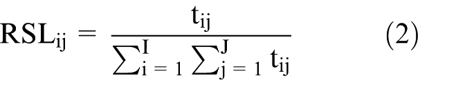
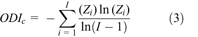
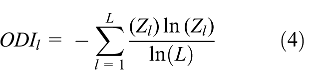
Different analytical methods exist to characterise the urban network by means of transportation networks. The method of complex network is widely used to explore the topological properties of transportation networks (e.g. degree centrality, betweenness centrality and closeness centrality) by means of transportation mode flows. Good examples are analyses of the Chinese airlines network (Wang et al., 2011, 2014), and the maritime network (Ducruet, 2013). Also, the reversed gravitation model has been used widely to estimate nodal attractions in cities from passenger flow volumes, for example the application of air passenger flows in the city nodes in China (Xiao et al., 2013). Although both methods are very useful, the method of complex network uses only the topological properties of cities in transportation networks as proxies for their importance in urban networks and neglects the importance of city pairs, while the reversed gravitation model does not measure the structure of a whole urban network. To understand the differences between the two types of HSR flow data in characterising the whole pattern of the urban network, a flow approach based on Limtanakool et al. (2007a) is used by situating HSR networks between the ideal-typical extremes of concentration and dispersal, and by focusing on the strength and the structure of urban networks. Regarding spatial effects of HSR networks, urban networks can thus be placed on a continuum ranging from a fully concentrated (monocentric) system in which time schedule/passenger flows are concentrated in one (or a few) dominant node(s), to a fully dispersed (polycentric) system in which there are no truly dominant nodes because time schedule/passenger flows are dispersed across urban areas (Figure 1). The strength of nodes and links is relevant to the position of a city or a link in the urban system. The structure defines the urban network, ranging from a fully monocentric to a fully polycentric structure. Neither passenger nor time schedule data include information on the origins or destinations of trips. 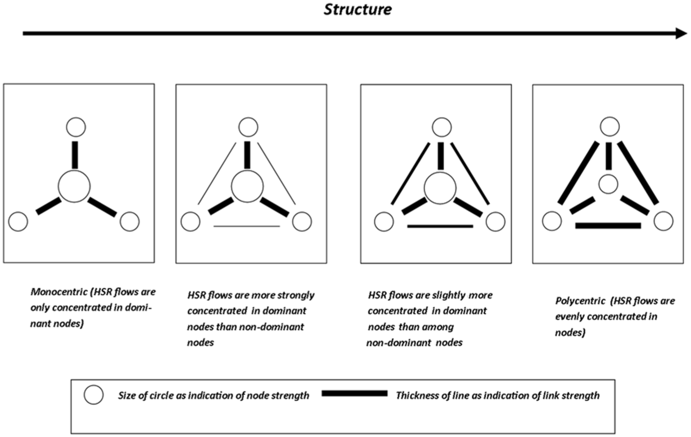In this article, two indices are used to measure the strength (the Dominance Index $DI T_{i}$ and the Relative Strength Index $RS L_{ij}),$ and two are used to measure the structure (Entropy Indices ODI_c; and ODI_l). These measures are defined at two levels: the individual node/link level and the network level.

Figure 1.

Conceptual model for HSR flows and urban networks.

$DI T_{i}$ and $RS L_{ij}$ are measures of the strength at the individual city/link level. At the individual city level, non-directional dominance $DI T_{i}$ calculates the ratio between the sum of the interactions associated with city I and the average extent of the interactions associated with other cities in the network. $RS L_{ij}$ is measured at the link level between a pair of cities and calculates the proportion of traffic interaction on a single link between a pair of cities relative to the total traffic interaction in the network:

DI T_{i} = \frac{T_{i}}{(\sum_{j = 1}^{J} T_{j} / J)}

(1)

RS L_{ij} = \frac{t_{ij}}{\sum_{i = 1}^{I} \sum_{j = 1}^{J} t_{ij}}

(2)

where $T_{i}$ is the total number of passengers/trains associated with city I, and i≠j. Cities with $DI T_{i}$ values above 1 are considered dominant because they are more important than the average of the other cities in the network; $t_{ij}$ is the total number of passengers/trains travelling between cities i and j, and i≠j. $RS L_{ij}$ is the value for all links in the network sum to unity, where individual values range from 0 to 1. A value of 1 indicates the highest strength of a link.

$OD I_{c}$ and $OD I_{l}$ are measured for the structure at the network level. $OD I_{c}$ (equation 3) is the measure that calculates the extent to which the total interaction is distributed evenly across all cities in the network. $OD I_{l}$ (equation 4) is the overall distribution index based on links, and it measures the extent to which the total interaction is distributed evenly across all links (city pairs) in the network.

OD I_{c} = - \sum_{i = 1}^{I} \frac{(Z_{i}) \ln (Z_{i})}{\ln (I - 1)}

(3)

OD I_{l} = - \sum_{l = 1}^{L} \frac{(Z_{l}) \ln (Z_{l})}{\ln (L)}

(4)

$Z_{i}$ is the share of passengers associated with city i within the total number of passengers/trains, and I is the number of cities in the network. $OD I_{c}$ ranges from 0 to 1. A value of 0 measures the highest hierarchical differential. $Z_{l}$ is the share of passengers/trains travelling on link l among the total number of passengers/trains, and L is the potential number of links in the network. $OD I_{l}$ ranges from 0 to 1. A value of 0 measures the highest hierarchical differential.

Data description and data comparison method

The Transportation Bureau of the China Railway Corporation collected the passenger flow data which are used in this study, including the incoming and outgoing numbers of D trains (average operational speed around 200 km/hour) and G trains (average operational speed around 300 km/hour) for O/D passengers travelling between pairs of cities. This data set covers the 106 existing HSR cities in China up to the end of 2013 (over 436 million passengers). Some cities, such as Tianjin and Jinan, have more than one HSR station, and the passenger numbers for multiple HSR stations have been merged for one city. Because seven cities with HSR stations were connected during 2013, we omitted those seven cities to have a complete overview of national HSR flows for the stations existing throughout 2013. In addition, some passengers transit in hub cities, such as Beijing and Guangzhou, to take another HSR train to their destination. In our data set, these journeys with a transfer are counted as two individual trips. Therefore, we acknowledge that, to some extent, passenger flow data may slightly misrepresent the actual number of passengers travelling from their origins to hub cities (or to non-hub cities).

Regarding the time schedule data, we used the Jipin time schedule for extracting only the daily frequency of HSR trains in 2013.¹ We collected the O/D train flows from the 12 months of 2013 for the same 99 cities as the acquired passenger flow O/D data set. The data sets include the number of all D+G trains from one city to the other in a matrix table. We then calculated the average daily HSR frequency from the time schedule data sets, including two types of HSR trains (G trains and D trains).

In total, we had 99 HSR cities and 1240 HSR connections for both types of data sets at the national scale. Both values were calculated for time schedule data as well as for passenger flow data to identify the differences in the rank of cities and links using two types of data sets.

Observed differences between the types of data will be explained by the attributes of city nodes and links. Three types of indices from the attributes of urban systems were chosen as potential determinants of the observed differences (Table 1). First, indicators for the socio-economic performance of cities have been chosen: GDP per capita, urban population and employment in the tertiary sector (Limtanakool et al., 2007b; Taylor, 2009). These indicators represent a measure of the potential travel demand of a given city. Due to the high correlation between tertiary employment and urban population, we have chosen tertiary employment given that HSR travel is orientated mainly towards tertiary industry in a city, such as the finance and estate sectors (Cheng et al., 2015). Second, the topological properties of transport networks are important (Reggiani and Nijkamp, 2007). These topological properties of transportation networks, i.e. degree centrality (DC), closeness centrality (CC) and betweenness centrality (BC), could reflect the direct connectivity, accessibility and transitivity of city nodes in the transportation networks, respectively (Wang et al., 2011). Because HSR travel is not a direct point-to-point connection compared to airline travel (Givoni and Dobruszkes, 2013), and there is a high correlation between CC and DC (Lin, 2012), we have chosen CC as an indicator. Cities with a high level of closeness centrality are able to attract or generate more operational transportation services (Lin, 2012); high betweenness centrality in the transportation network allows a city node to broker more flows and serve as a crucial hub (Borgatti et al., 2009). Third, institutional factors have been identified as potential indicators of activities that are likely to generate transportation flows. We assume that the railway hub status of a city given by the central government could play an important role in the provision of HSR trains (Jin et al., 2010). This indicator is different from BC, since it reflects the hub status of cities from a planning perspective in the whole railway system rather than from an operational perspective in the HSR network. In addition, the higher the position of a city in the administrative hierarchy, the more likely it is that people, especially civil servants living in that city, would travel to other cities via transportation networks (Dobruszkes et al., 2011). To reflect the attributes of city links, we used the summed attributes of city nodes as indicators for a link. The variable of summed BC was not used for the difference in link strength because of its high correlation with tertiary employment (r = 0.84). A classical, linear multiple regression model was drawn up using the ‘stepwise’ method to determine significant variables that are useful to include in the model to explain the differences between the two types of data in city strength and link strength. Scatterplot analysis was applied to characterise the cities and links for which time schedule data are not robust (unacceptable over- or underestimation) proxies for passenger flow data.

Table 1.

Variables for the scatterplot analysis.

Variables	Explanation	Min–Max values	Mean value
Dependent variables
Difference in city strength	$DIF_DI T_{i} = DI T_{i}_time schedule - DI T_{i}_passenger$ $DIF_DI T_{i} \in (- \infty, + \infty)$ , whereby < 0 means the city strength of time schedule data underestimate the city strength of passenger flow data. > 0 means the city strength of time schedule data overestimate the city strength of passenger flow data. = 0 means the city strength of time schedule data is equal to the city strength of passenger flow data	−4.72–1.32	−0.014
Difference in link strength	$DIF_RS L_{ij} = RS L_{ij}_time schedule - RS L_{ij}_passenger$ $DIF_RS L_{ij} \in (- \infty, + \infty)$ , whereby < 0 means the link strength of time schedule data underestimate the link strength of passenger flow data. > 0 means the link strength of time schedule data overestimate the link strength of passenger flow data. = 0 means the link strength of time schedule data is equal to the link strength of passenger flow data	−4.552–0.827	0.004
Independent variables at city level
GDP per capita*	City’s GDP per capita in 2013 (yuan)	15,801.98–466,996.1	66,886.32
Tertiary employment*	City’s employees in the tertiary sector in 2013 (10,000 persons)	2.06–564.73	41.99
BC	$C_{B} (i) = \sum_{k \neq i \neq j \neq N} σ_{k j} \frac{(i)}{σ_{k j}}$ where $σ_{kj}$ is the sum of all shortest paths between nodes k and j, and $σ_{kj}$ (i) is the number of shortest paths that pass through i. It reflects the extent to which a particular city node lies between other nodes in a network, indicating the transitivity	0–1189.374	51.03
CC	$C_{C} (i) = \frac{n - 1}{\sum_{υ_{j} \in V, i \neq j} d_{ij}}$ where d_ij is the number of edges for the shortest path from i to j, and n is the number of city nodes. It measures the extent to which a node is close to all other nodes along the shortest path and reflects its accessibility in a given transportation network	0.198–0.742	0.51
Hub status	Railway hub status: 0 = non-hub city and 1 = hub city, which is defined according to Jin et al. (2010)	0–1	0.15
Administrative level	Hierarchical administrative level (scored) 1 = municipality city, 2 = sub-provincial/regional capital city, 3 = prefecture city and 4 = county city, which is defined according to Ma (2005)	1–4	2.72
Independent variables at link level
GDP per capita – Sum	Summed GDP per capita number of two connected cities in a link	35,599.95–652,267.6	148,959.9
Tertiary employment – Sum	Summed urban population number of two connected cities in a link	11.13–939.66	533.6
CC – Sum	Summed CC value of two connected cities in a link	0.44–1.41	178.59
Hub status – Sum	Summed value of two connected cities’ hub status in a link	0–2	1.11
Administrative level – Sum	Summed value of two connected cities’ administrative level in a link	2–8	5.27

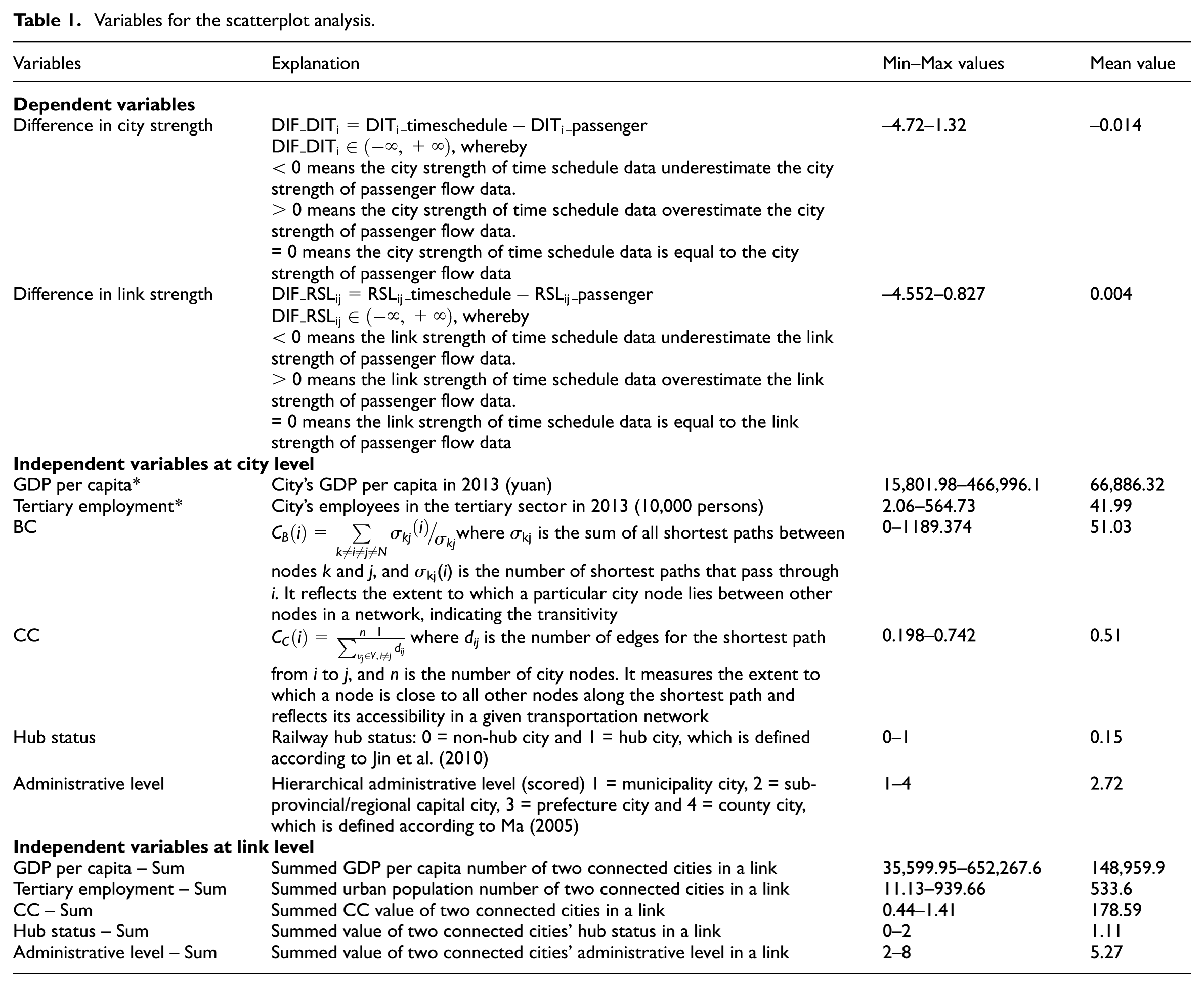
The scatterplot (Figure 2) can be divided into six parts: the upper left and right parts, the middle left and right parts and the lower left and right parts. The Y-axis represents the dependent variable, the difference in city strength or link strength. The X-axis represents the relevant significant independent node/link attributes from the regression model. Based on the three sigma rule of statistics (Pukelsheim, 1994), we define the mean value plus and minus one standard deviation for the Y-axis as the lower and upper limit values to delimit the values of time schedule data, which represent passenger data (the middle parts) reasonably well. In this study, if the differences between the two types of data (passenger flow and time schedule data) in city strength and link strength are above one standard deviation, then the difference between the two types of data sets is considered too large. This means that in this situation, the use of time schedule data will lead to unacceptable over- or underestimation of city/link strength of deviant cities/links in the upper or lower parts. The remaining normal cities located in the middle parts mean that time schedule data represent passenger flow data for identifying city and link strength. Furthermore, to differentiate the typical characteristics of deviant cities from those of normal cities, we define the mean value plus one standard deviation for the X-axis as the threshold value for the node/link attributes to identify how the overestimation or underestimation cases are related to the attributes of nodes or links of urban systems.

Figure 2.

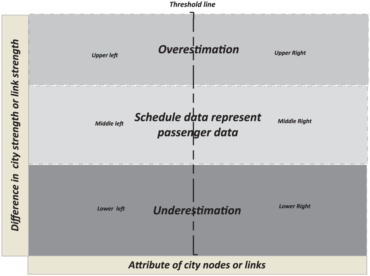
Scatterplot part.

Empirical results for the two types of HSR data sets on the strength and structure of urban networks

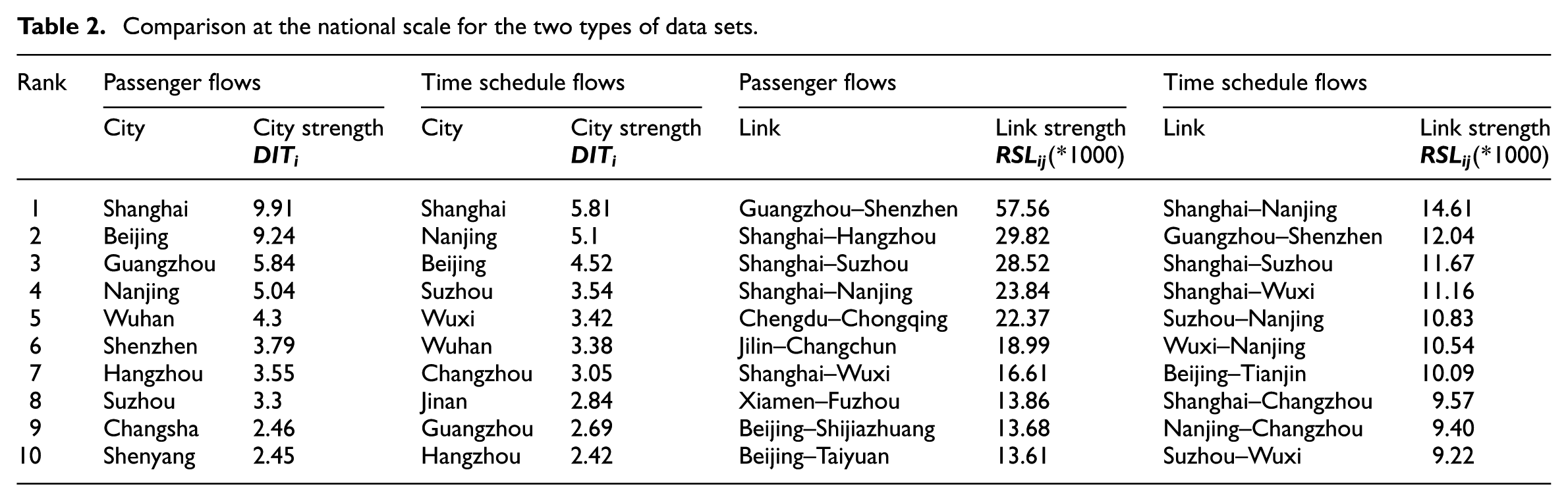
First, we compared the two types of data sets at the national scale to see how HSR networks determine the configuration of urban networks, whether with concentration or dispersal effects. The top 10 dominant cities with a value of $DI T_{i}$ larger than 1, and the accumulated value of the top 10 links, were noted (see Table 2). Derived from this analysis, Table 3 directly lists the ranking change of the cities.

Table 2.

Comparison at the national scale for the two types of data sets.

Rank	Passenger flows		Time schedule flows		Passenger flows		Time schedule flows
	City	City strength $DI T_{i}$	City	City strength $DI T_{i}$	Link	Link strength $RS L_{ij}$ (*1000)	Link	Link strength $RS L_{ij}$ (*1000)
1	Shanghai	9.91	Shanghai	5.81	Guangzhou–Shenzhen	57.56	Shanghai–Nanjing	14.61
2	Beijing	9.24	Nanjing	5.1	Shanghai–Hangzhou	29.82	Guangzhou–Shenzhen	12.04
3	Guangzhou	5.84	Beijing	4.52	Shanghai–Suzhou	28.52	Shanghai–Suzhou	11.67
4	Nanjing	5.04	Suzhou	3.54	Shanghai–Nanjing	23.84	Shanghai–Wuxi	11.16
5	Wuhan	4.3	Wuxi	3.42	Chengdu–Chongqing	22.37	Suzhou–Nanjing	10.83
6	Shenzhen	3.79	Wuhan	3.38	Jilin–Changchun	18.99	Wuxi–Nanjing	10.54
7	Hangzhou	3.55	Changzhou	3.05	Shanghai–Wuxi	16.61	Beijing–Tianjin	10.09
8	Suzhou	3.3	Jinan	2.84	Xiamen–Fuzhou	13.86	Shanghai–Changzhou	9.57
9	Changsha	2.46	Guangzhou	2.69	Beijing–Shijiazhuang	13.68	Nanjing–Changzhou	9.40
10	Shenyang	2.45	Hangzhou	2.42	Beijing–Taiyuan	13.61	Suzhou–Wuxi	9.22

Table 3.

Rank of cities using passenger flow and time schedule data.

City	Passenger flows		Time schedule flows		Change in rank
	Rank	$DI T_{i}$ city strength	Rank	$DI T_{i}$ city strength
Shanghai	1	9.91	1	5.81	0
Beijing	2	9.24	3	4.52	−1
Guangzhou	3	5.84	9	2.69	−6
Nanjing	4	5.04	2	5.10	2
Wuhan	5	4.30	6	2.42	−1
Shenzhen	6	3.79	30	1.17	−24
Hangzhou	7	3.55	10	2.42	−3
Suzhou	8	3.30	4	3.54	4
Changsha	9	2.46	12	2.29	−3
Shenyang	10	2.45	17	1.57	−7
Wuxi	11	2.42	5	3.42	6
Jinan	12	2.33	8	2.84	4
Zhengzhou	13	2.23	13	2.23	0
Fuzhou	14	1.98	18	1.54	−4
Xiamen	15	1.88	27	1.19	−12

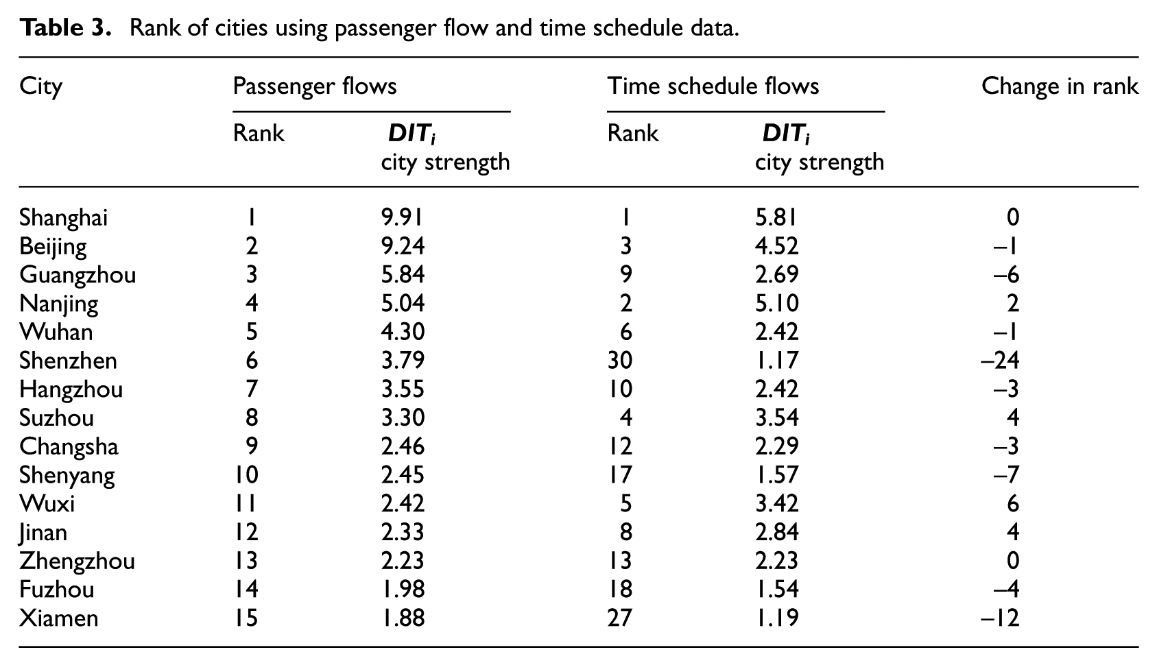
With regard to the city strength $DI T_{i}$ , Shanghai, Beijing and Guangzhou are the top three dominant cities using passenger flow data, whereas Nanjing replaces Beijing in second place using time schedule data. There are obvious ranking changes from the passenger flow data to the time schedule data in Table 2. For example, Guangzhou and Shenzhen rank third and sixth in the passenger flow data but drop to ninth and 30th, respectively, in the time schedule data. Nanjing and Suzhou rank fourth and eighth in the passenger flow data but rise to second and fourth, respectively, in the time schedule data. This reflects the large differences in ranking the importance of cities in HSR networks when using the two different types of data. Compared with the national network of passenger flow data, with 28 dominant cities ( $DI T_{i}$ city strength larger than 1), that of the time schedule data has 35 dominant cities. Furthermore, there are smaller differences between the values of $DI T_{i}$ in the dominant cities in the national HSR network of the time schedule data. With regard to link strength, the accumulated value of the top 10 links in the national network of the time schedule data (109.14) is much smaller than that of the passenger flow data (238.86), indicating that the national network derived from the time schedule data appears to be less hierarchical than the one derived from passenger flow data.

Table 4 shows the structure values for passenger and time schedule data. With regard to the city structure ODI_c, the city networks of both data sets show a less hierarchical configuration, whereas the city network level of the passenger flow data is more hierarchical than that of the time schedule data. Regarding the link structure ODI_l, the link networks of both data sets show a hierarchical configuration, whereas the link network level of passenger flows is more hierarchical than that of the time schedule data as well.

Table 4.

Structure values for the two types of data sets.

Structure values	Passenger flows	Time schedule flows
$OD I_{c}$	0.84	0.90
$OD I_{l}$	0.42	0.49

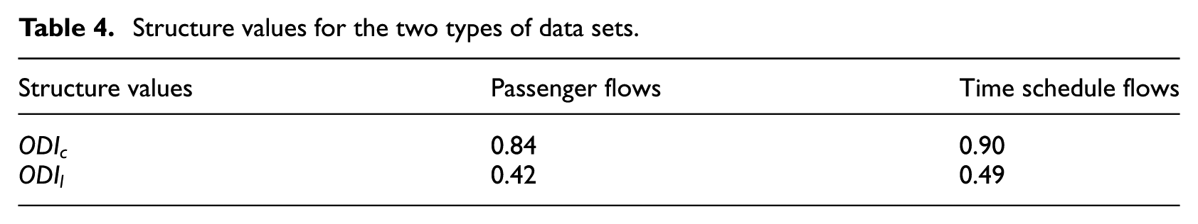
In summary, large differences were found between the two types of HSR flow data at the national scale when determining the hierarchical positions of cities and links. The time schedule data represent a picture of less hierarchical urban networks in that there are fewer dominant cities and smaller accumulated values of top 10 link strength compared with the passenger flow data. That also means that even though the operational companies arrange an average number of HSR trains between cities to pursue dispersal effects of HSR networks on national urban networks, the HSR networks would still contribute to more concentration effects regarding actual travel demand. This is in accordance with the structure values of national urban networks, which confirm that the structure values of two types of data at the city network level present a polycentric network, whereas those of the time schedule data are less hierarchical than those of the passenger flow data. In light of this, in the next section we delve further into the relationships between the differences of the two types of data in characterising urban networks and the attributes of city nodes and links.

Results of the multiple regression

When using the difference in city strength as a dependent variable, three variables contribute significantly in predicting variations of the difference in city strength between the two types of data. These are GDP per capita, especially tertiary employment, and CC (Table 5), with tertiary employment as the most important determinant. The other variables chosen are less useful in accounting for differences in city strength for our set of cities.

Table 5.

Multiple regressions results.

Variables	Difference in city strength	Variables	Difference in link strength
	Beta Coef.		Beta Coef.
Tertiary employment	−0.687***	Summed tertiary employment	−0.284***
GDP per capita	−0.267***	Summed GDP per capita	−0.129***
Closeness centrality (CC)	0.154**	Summed CC	0.214***
Betweenness centrality (BC)	x	Summed hub status	−0.078**
Hub status	x	Summed administrative level	x
Administrative level	x
Observations	99		1240
Adjusted R-squared	0.652		0.131

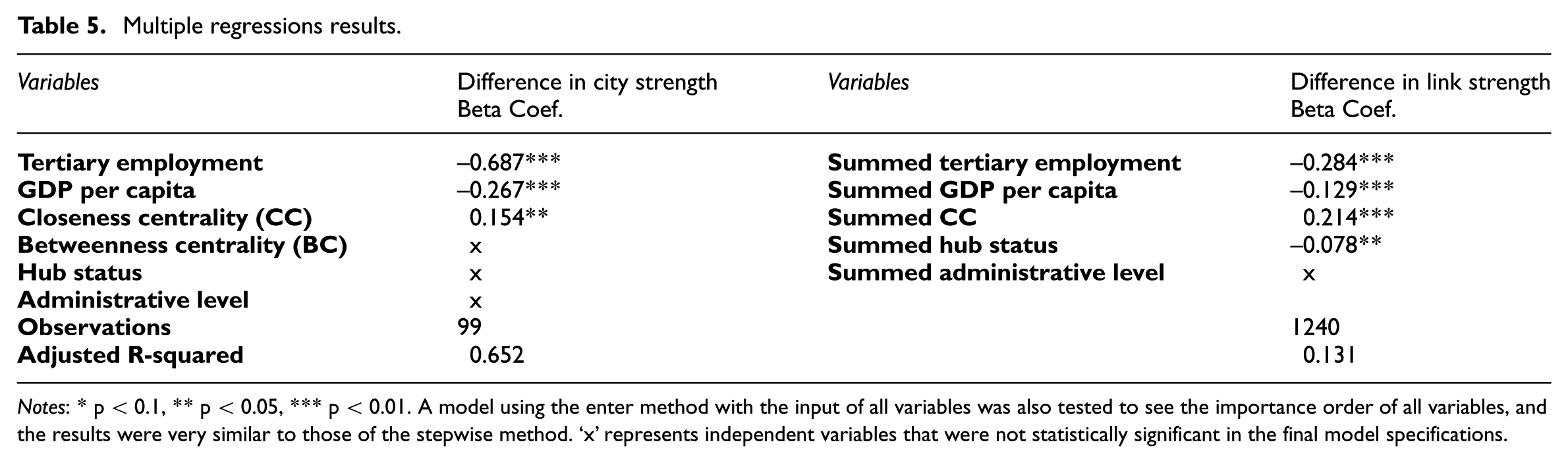
Notes: * p < 0.1, ** p < 0.05, *** p < 0.01. A model using the enter method with the input of all variables was also tested to see the importance order of all variables, and the results were very similar to those of the stepwise method. ‘x’ represents independent variables that were not statistically significant in the final model specifications.

By comparison, the regression model that describes the difference in link strength yields the same socio-economic and typological variables as above (summed tertiary employment, summed GDP per capita, summed CC), but with one different institutional variable (summed hub status), and summed tertiary employment being the most important determinant. Although these four variables account for less than 14% of the variation in the difference in link strength, our major focus here is to only select the most relevant socio-economic, typological and institutional attributes of city pairs for the next scatterplot analysis instead of fully explaining the differences in link strength. To make sure the results of our selected variables are consistent, we have also tried another variable selection method to improve the explanation power of the model – the least absolute shrinkage and selection operator (LASSO) model – to test all of the predictors. The LASSO model is more efficient for removing DC with high correlations to CC from the final selected model than doing it by ourselves in the section of comparison methods. However, the final explanation power of the LASSO model (13.6%) in link strength is almost the same as the stepwise model and the importance order of final selected variables is the same as the stepwise model. It might be that the capacity (passenger loading and unloading volumes) and the number of carriages of trains that are not covered by the time schedule data are more important in explaining variations in link strength differences between the two types of data. However, data on these variables are not accessible.

Results of the scatterplot analysis

We used scatterplots to observe and interpret the interaction between determinant attributes and the differences of the values of city and link strength to clarify the typical characteristics of cities and links to which the time schedule data could unacceptably underestimate or overestimate the passenger flow data. Based on the regression analyses (Table 5), we have chosen the determinant-independent variables, i.e. tertiary employment, GDP per capita and CC at the city level, and summed tertiary employment, CC, GDP per capita and hub status at the link level.

City level

In the scatterplots of Figure 3, the Y-axis represents the dependent variable (the difference between two types of data in city strength) and the X-axis represents the relevant independent variables. The critical range for the Y-axis (–1.06, 0.77) is defined as the values between the mean value of the difference in city strength plus and minus one standard deviation, and the threshold values for the X-axis (tertiary employment of 1.41 million persons, GDP per capita of 124.450 and CC of 0.6) are defined as the mean value of each factor plus one standard deviation. In the middle parts of the scatterplots are cities for which time schedule data are reasonably good representations of passenger data. Compared with the use of passenger flow data, for ‘deviant cities’ in the lower or upper parts of the scatterplots with values of difference in city strength outside this range, the use of time schedule data leads to an unacceptable under- or overestimation of actual city strength. In total, there are six and seven deviant cities in the lower and upper parts, respectively; the rest of the 86 normal cities are in the middle parts.² Given that tertiary employment and GDP per capita exert negative impacts, and CC a positive impact on the difference in city strength, we visualised the deviant cities beyond the threshold values of tertiary employment and GDP per capita, and under the threshold value of CC in the lower shaded parts, and the deviant links under the threshold values of tertiary employment and GDP per capita, and beyond the threshold value of CC in the upper shaded parts of Figure 3.

Figure 3.

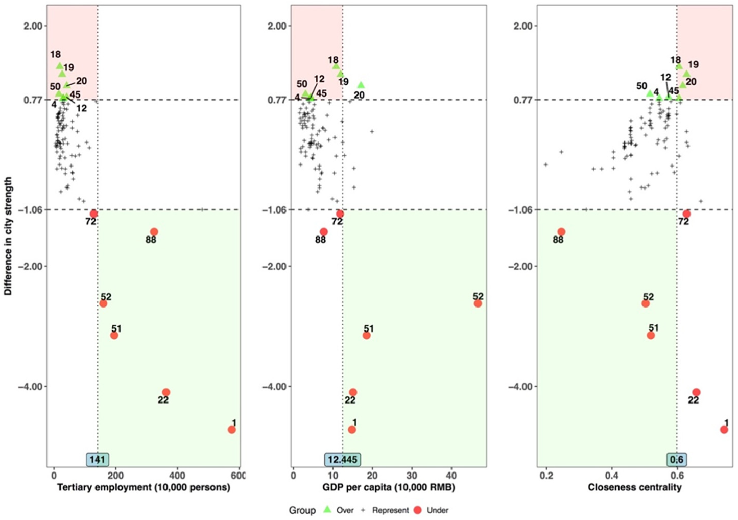
Scatterplot analysis on the difference in city strength.

By taking into consideration the most determinant socio-economic indicators (tertiary employment and GDP per capita), only four out of six deviant cities are beyond both threshold values (i.e. Beijing (1), Shanghai (22), Guangzhou (51) and Shenzhen (52)) in the lower shaded parts of the relevant scatterplots. This reflects that the city strength of cities with the characteristic of high socio-economic performance tends to be unacceptably underestimated by time schedule data. As the widely acknowledged top four ranked cities in the Chinese urban system, these first-tier class cities in China with much larger tertiary employment are able to generate higher travel demand than other cities with lower tertiary employment (Cheng et al., 2015). Besides, passengers living in cities with a much larger GDP per capita are more likely to be able to afford the monetary travel cost, considering the expensive prices of HSR tickets (Liu and Kesteloot, 2015). Consequently, it can be expected that the capacity of trains to and from these cities, which is not reflected in the time schedule, is much higher than for other cities, thus leading to a considerable underestimation of their city strength.

By comparison, the cities under the threshold values of tertiary employment and GDP per capita include not only six out of a total of seven deviant cities in the lower parts, i.e. Dezhou (4), Xuzhou (12), Zhenjiang (18), Changzhou (19), Yueyang (45) and Shaoguan (50), but also 81 of a total of 86 normal cities in the middle parts, with time schedule data representing passenger flow data. The high percentages of both deviant cities (86%) and normal cities (94%) with low socio-economic performance indicate that a city with the characteristic of low socio-economic performance will not necessarily be a deviant city whose city strength tends to be unacceptably overestimated by time schedule data. The reason could be that although cities with relatively low socio-economic performance are less likely to generate large travel demand, there is still a high chance that the supply of HSR services to/from those cities is also rather low because of their low socio-economic performance. Thus, it is necessary to take into account the attribute of CC to differentiate the typical characteristics of deviant cities from those of normal cities, although the contribution of CC is limited. By further taking into account the cities beyond the threshold value of CC, we find that the cities in all three scatterplots (Figure 3) are the only deviant cities – Zhengzhou (18), Changzhou (19) and Yueyang (45) – in the upper shaded parts of the scatterplots, whose accessibility levels are much higher than other cities in the HSR network. This indicates that time schedule data tend to overestimate the importance of cities with relatively low values of tertiary employment and GDP per capita only when their accessibility levels are much better in the transportation network. These cities with much better accessibility in HSR networks have a higher frequency of HSR trains compared with other cities (Jiao et al., 2017), which is not supported by their rather low levels of travel demand.

In sum, on the one hand, when cities’ tertiary employment and GDP per capita are much higher than their threshold values, their city strength tends to be largely underestimated by time schedule data. On the other hand, when the accessibility of cities with relatively low socio-economic performance is much higher than the threshold value of the transportation network, their city strength tends to be severely overestimated by time schedule data.

Link level

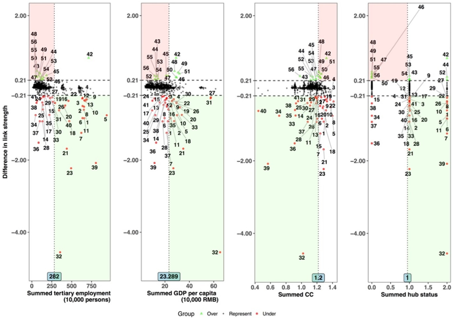
In the scatterplots of Figure 4, the critical range (–0.21, 0.21) for the Y-axis is defined as the values between the mean value of the difference in link strength plus and minus one standard deviation; the threshold values for the X-axis (summed tertiary employment of 282 million persons, summed GDP per capita of 232.892 RMB, summed CC of 1.2 and summed hub status of 1) are defined as the mean value of each factor plus one standard deviation. Deviant links within the range 0.21–0.83 in the upper parts represent links for which time schedule data considerably overestimate the link strength of the passenger flow data, while deviant links within the range 4.55–0.21 in the lower parts reflect that time schedule data greatly underestimate the link strength by passenger flow data. In total, there are 15 and 41 deviant links in the upper and lower parts, respectively; the rest of the 1184 normal links are in the middle parts. Considering that summed tertiary employment, GDP per capita and hub status exert negative impacts and summed CC a positive impact on the difference in link strength, we visualised the deviant links beyond the threshold values of the summed tertiary employment, summed GDP per capita and summed hub status, and under the threshold value of summed CC in the lower shaded parts, and the ones under the threshold values of summed tertiary employment, summed GDP per capita and summed hub status, and beyond the threshold value of summed CC in the upper shaded parts of Figure 4.

Figure 4.

Scatterplot analysis on the difference in link strength.

By only taking into account the most determinant socio-economic indicators (summed tertiary employment and summed GDP per capita), the links beyond the threshold values include not only 11 out of a total 41 deviant links in the lower parts of the scatterplots (i.e. Guangzhou–Shenzhen (32), Wuhan–Guangzhou (26), Shanghai–Hangzhou (23), Shanghai–Wuhan (22), Suzhou–Shanghai (21), Wuxi–Shanghai (20), Nanjing–Shanghai (18), Beijing–Shenyang (11), Beijing–Wuhan (10), Beijing–Shanghai (5), Beijing–Nanjing (4), Beijing–Qingdao (2) and Beijing–Jinan (1)), but also 24 out of a total of 1184 normal links in the middle parts. Regarding a much higher percentage of links with high socio-economic performance to be a deviant city (30%) in the lower shaded parts than a normal city (2%) in the middle parts, links with the characteristic of high socio-economic performance tend to be largely overestimated by time schedule data. Obviously those deviant links are links in China whose city ends serve as socio-economic cores, and major cities in specific regions; for instance, Beijing and Shanghai are socio-economic cores, in the Bohai Rim and YRD regions, and Guangzhou and Shenzhen are the cores in the PRD region, having strong functional interactions with each other and other major cities such as Shenyang, Hangzhou and Nanjing. Therefore, to satisfy the above average demand of passengers travelling between those city nodes, with regards to the maximum capacity of operating trains in the railway systems, operation companies provide relevant routes between city nodes with longer trains that offer more seats, which are not reflected in the time schedule data. If we further consider the attributes ‘summed CC’ and ‘summed hub status’, the links in all four scatterplots in Figure 4 concern only deviant links, i.e. Guangzhou–Shenzhen (32) and Wuhan–Guangzhou (26), in the lower shaded parts. For these links, besides the intense functional interactions between the linked socio-economic cores, these cores also serve as railway hubs in China, meaning that next to original passengers travelling for functional activities in those cores, as hubs they can also generate additional passengers in between for their next transit trips by conventional railways (Jin et al., 2010). However, due to a low level of accessibility of the links in the HSR network, operational companies only provide the relevant routes with a fewer than average supply of HSR trains with more carriages and seats to satisfy the additional travel demand for transit trips, which will lead further to an unacceptable underestimation of the link strength by time schedule data.

By comparison, the links under the threshold values of summed tertiary employment and summed GDP per capita are not only 10 out of a total of 15 deviant links in the upper parts of the scatterplots, i.e. Putian–Quanzhou (56), Changsha–Shaoguan (55), Wuhan–Shaoguan (54), Wuhan–Chenzhou (53), Shijiazhuang–Zhengzhou (52), Zhenjiang–Changzhou (47), Jinan–Nanjing (45), Jinan–Xuzhou (44) and Cangzhou–Jinan (43), but also 975 out of a total of 1184 normal links in the middle parts. Regarding the high percentages of both deviant cities (67%) and normal cities (82%) with low socio-economic performance, this also indicates that the city link with the characteristic of low socio-economic performance will definitely not be a deviant link to which time schedule data largely overestimate passenger data. Therefore, it is necessary to take into account other determinant attributes to characterise the deviant links. By further considering summed hub status and summed CC, there is only one deviant link in the upper shaded parts of all four scatterplots of Figure 4, Zhenjiang–Changzhou (47), with quite a high level of accessibility and linked city ends being non-railway hubs. As opposed to Wuhan–Guangzhou (26) and Guangzhou–Shenzhen (32) in the lower shaded parts of all four scatterplots, as two non-railway hubs, Zhengjiang and Changzhou with low socio-economic performance would be less likely to generate passengers travelling in between for functional activities and following transit trips. Meanwhile, both linked city ends with a high level of accessibility in the HSR network are able to receive a larger than average supply of HSR services in between. As a consequence, the situation of a high frequency of HSR trains with low capacity running through the relevant routes will give rise to an excessive overestimation of the link strength by time schedule data.

In sum, the link strength of city links with city ends of high socio-economic performance in respective regions has a high chance of being underestimated by time schedule data. Furthermore, for links with city ends serving as railway hubs and having relatively low accessibility in the transportation network, the link strength between these city ends is even more underestimated by time schedule data. In contrast, the link strength between cities with relatively low socio-economic performance, which serve as non-railway hubs, and which are highly accessible in the transportation network, is severely overestimated by time schedule data.

Conclusion and discussion

Large differences exist between passenger and time schedule data for measuring the configuration of urban networks connected by HSR networks, due to the intrinsic nature of the two types of data representing market demand and supply. To the best of our knowledge, this article is the first study to apply the same original indices of a model proposed by Limtanakool et al. (2007a) (the strength of cities and links and the structure of city and link networks) to compare two types of HSR flow data in the characterisation of urban networks regarding spatial concentration and dispersal effects of HSR networks. Then, according to the most determinant attributes of urban systems for explaining the differences between the two types of flow data, we identified the typical characteristics of urban systems in which time schedule data is not a good proxy for passenger flow data by means of scatterplot analysis.

This research indicates small differences for the empirical analysis on the structure of city and link networks in China but significant differences between passenger data and time schedule data on ranking the city nodes and links. Both the structures of the city networks and of the link networks show the same configurations (less hierarchical at the city network level and hierarchical at the link network level); however, those of passenger flows are all more hierarchical than those of time schedule flows. This further reflects that even though the Chinese government aims to balance the development of regions by supplying a high frequency of HSR trains between cities (Jiao et al., 2017), the relevant configuration of urban networks still tends to present a more hierarchical structure regarding actual HSR travel demand. In other words, HSR networks would in fact contribute more concentration effects reflected from the demand side than dispersal effects expected from the supply side on national urban networks. The most determinant indicators for explaining the differences in city and link strength are socio-economic factors (tertiary employment and GDP per capita), followed by the cities’ topological properties in HSR networks (closeness centrality) and institutional factors (hub status). The strength values of city nodes and links with low socio-economic performance are not necessarily related to an unacceptable overestimation by time schedule data. The reason could be related to their low socio-economic performance with a low travel demand; operational companies correspondingly provide them with a small supply of HSR services. However, if these city nodes and links are highly accessible in HSR networks, their strength values tend to be largely overestimated by time schedule data, especially when linked city nodes are not hubs in the conventional railway network. The reason could be that Chinese HSR networks, which were inaugurated in 2003 and are expected to be completed in 2020, aim to improve the accessibility of Chinese cities in the railway network, especially cities with low socio-economic performance, to realise the integration of different regions, even those with rather low passenger flows between these cities in the first few years. As a result, based on time schedule data, the importance of these city nodes is overestimated in the HSR and national urban networks, and the concentration effects of HSR networks on those cities would not be what is expected by the government (Wu et al., 2014). On the other hand, cities with a city strength unacceptably underestimated by time schedule data are major first-tier cities in China with high tertiary employment and GDP per capita. City links with a link strength unacceptably underestimated by time schedule data normally connect socio-economic core cities and other major cities within their respective regions at different spatial scales. This might be a result of a larger than average capacity in trains running to and from these major tier cities compared with lower-tier cities, to satisfy the demands of passenger travel. That also means that HSR networks would actually exert concentration effects on those cities, rather than the dispersal effects expected by the government, with the aim of integration of those cities with other lower-tier cities. In addition, if these major tier cities are not highly accessible in the HSR network but still serve as railway hubs, it will further lead to an excessive underestimation of the link strength between those city nodes, as a result of an even lower supply of HSR services, with more carriages and seats to satisfy a larger travel demand, including original passengers for functional activities in/between these cities and additional passengers for their next transit trips. Unfortunately, these data were not available to us.

In light of the case study of HSR networks in China, a comparative analysis was developed on Chinese urban networks between passenger and time schedule data. With regard to the high accessibility of time schedule data, we cannot deny the usefulness of the application of time schedule data in characterising urban networks. However, urban geographers and transportation planners should bear in mind that the large differences found in the city and link strengths based on the two types of HSR flow data are strongly related to the socio-economic status of city nodes connected by HSR, especially for major city nodes with large passenger demand. When analysing the spatial structure of HSR and urban networks by means of the flow approach, it is necessary for experts to consider not only the frequency of transportation modes but also, more importantly, the capacity of each carriage in the absence of actual passenger flow data. This is especially true for cities and regions with large tertiary employment, and GDP per capita such that of as Beijing and Shanghai, and the links between them may be largely underestimated by the time schedule data. Furthermore, the findings on the differences in the empirical results of the two types of HSR flow data generate interesting future research questions concerning whether they are applicable to other urban networks (e.g. those of France and Germany) that have built up complete HSR networks, or to other high-speed transportation mode networks (e.g. airlines) or even to other dimensions of networks such as symmetry.

Footnotes

Declaration of conflicting interests

The author(s) declared no potential conflicts of interest with respect to the research, authorship, and/or publication of this article.

Funding

The author(s) disclosed receipt of the following financial support for the research, authorship, and/or publication of this article: The authors thank the China Scholarship Council (Grant No. 201307720058) and National Natural Science Foundation of China (Grant No. 41722103) for supporting this research.

Notes

References

Borgatti

Mehra

Brass

et al . (2009) Network analysis in the social sciences. Science323: 892–896.

Brueckner

(2003) Airline traffic and urban economic development. Urban Studies40(8): 1455–1469.

Burghouwt

Hakfoort

Van Eck

(2003) The spatial configuration of airline networks in Europe. Journal of Air Transport Management9: 309–323.

Cheng

Loo

BPY

Vickerman

(2015) High-speed rail networks, economic integration and regional specialisation in China and Europe. Travel Behaviour and Society2(1): 1–14.

Derudder

Witlox

(2009) The impact of progressive liberalization on the spatiality of airline networks: A measurement framework based on the assessment of hierarchical differentiation. Journal of Transport Geography17(4): 276–284.

Derudder

Timberlake

Witlox

(2010) Introduction: Mapping changes in urban systems. Urban Studies47(9): 1835–1841.

Derudder

Witlox

Taylor

et al . (2003) Hierarchical tendencies and regional patterns in the World City network: A global urban analysis of 234 cities. Regional Studies37(9): 875–886.

Diao

Zhu

(2017) Intra-city access to inter-city transport nodes: The implications of high-speed-rail station locations for the urban development of Chinese cities. Urban Studies54(10): 2249–2267.

Dobruszkes

Lennert

Van Hamme

(2011) An analysis of the determinants of air traffic volume for European metropolitan areas. Journal of Transport Geography19(4): 755–762.

10.

Ducruet

(2013) Network diversity and maritime flows. Journal of Transport Geography30: 77–88.

11.

Feng

Xie

et al . (2014) Functional polycentricity of the urban region in the Zhujiang River Delta based on intercity rail traffic flow. Scientia Geographica Sinica 34: 648–655.

12.

Givoni

Dobruszkes

(2013) A review of ex-post evidence for mode substitution and induced demand following the introduction of high-speed rail. Transport Reviews33(6): 720–742.

13.

Green

(2007) Functional polycentricity: A formal definition in terms of social network analysis. Urban Studies44(11): 2077–2103.

14.

Hall

Pain

(2006) The Polycentric Metropolis: Learning from Mega-City Regions in Europe. London: Routledge.

15.

Jiao

Wang

Jin

(2017) Impacts of high-speed rail lines on the city network in China. Journal of Transport Geography60: 1–17.

16.

Jin

Wang

et al . (2010) China’s regional transport dominance: Density, proximity, and accessibility. Journal of Geographical Sciences20(2): 295–309.

17.

Limtanakool

Schwanen

Dijst

(2007a) A theoretical framework and methodology for characterising national urban systems on the basis of flows of people: Empirical evidence for France and Germany. Urban Studies44: 2123–2145.

18.

Limtanakool

Schwanen

Dijst

(2007b) Ranking functional urban regions: A comparison of interaction and node attribute data. Cities24(1): 26–42.

19.

Lin

(2012) Network analysis of China’s aviation system, statistical and spatial structure. Journal of Transport Geography22: 109–117.

20.

Liu

Kesteloot

(2015) High-speed rail and rural livelihood: The Wuhan–Guangzhou line and Qiya village. Tijdschrift voor economische en sociale geografie107(4): 469–483.

21.

Liu

Song

et al . (2015) Understanding urban China with open data. Cities47: 53–61.

22.

Luo

(2010) Study on the functional polycentricity of Yangtze River Delta [in Chinese].Urban Planning International25(1): 60–65.

23.

LJC

(2005) Urban administrative restructuring, changing scale relations and local economic development in China. Political Geography24(4): 477–497.

24.

Meijers

(2005) Polycentric urban regions and the quest for synergy: Is a network of cities more than the sum of the parts?Urban Studies42(4): 765–781.

25.

Neal

(2010) Refining the air traffic approach to city networks. Urban Studies47(10): 2195–2215.

26.

Pukelsheim

(1994) The three sigma rule. The American Statistician48(2): 88–91.

27.

Reggiani

Nijkamp

(2007) Transport networks and metropolitan development: New analytical departures. Networks and Spatial Economics7(4): 297–300.

28.

Taylor

(2004) World City Network: A Global Urban Analysis. London: Routledge.

29.

Taylor

(2009) Urban economics in thrall to Christaller: A misguided search for city hierarchies in external urban relations. Environment and Planning A41(11): 2550–2555.

30.

Van Nuffel

Saey

Derudder

et al . (2010) Measuring hierarchical differentiation: Connectivity and dominance in the European urban network. Transportation Planning and Technology33(4): 343–366.

31.

Wang

et al . (2011) Exploring the network structure and nodal centrality of China’s air transport network: A complex network approach. Journal of Transport Geography19(4): 712–721.

32.

Wang

(2014) Evolution of air transport network of China 1930–2012. Journal of Transport Geography40: 145–158.

33.

Nash

Wang

(2014) Is high speed rail an appropriate solution to China’s rail capacity problems?Journal of Transport Geography40: 100–111.

34.

Xiao

Wang

Liu

et al . (2013) Reconstructing gravitational attractions of major cities in China from air passenger flow data, 2001–2008: A particle swarm optimization approach. The Professional Geographer65(2): 265–282.

Comparing passenger flow and time schedule data to analyse High-Speed Railways and urban networks in China

Abstract

Keywords

Introduction

Understanding the external functional relationships of urban networks using different flow approaches

Background

Analytical framework

Data description and data comparison method

Empirical results for the two types of HSR data sets on the strength and structure of urban networks

Results of the multiple regression

Results of the scatterplot analysis

City level

Link level

Conclusion and discussion

Footnotes

Declaration of conflicting interests

Funding

Notes

References