
Abstract
Permeability measurement of easily deformable porous materials saturated with liquids represents a costly and time-consuming process, usually performed with complex experimental devices. This study proposes an alternative approach for evaluating the in-plane permeability of 3D warp-knitted spacer fabrics under compression. A 3D model was reconstructed from scanned images, and its behavior was analyzed using the finite-element method. The resulting deformed shapes of the representative cell were used in computational fluid dynamics simulation to assess the permeability across a wide compression range, approaching the densification phase. The permeability was determined from Darcy’s law at reduced flow speeds, whereas higher flow speeds were analyzed using the quadratic extension (Forchheimer) of the linear regime. Finally, simulation results at various compression ratios showed good agreement with experimental measurements, thus validating the numerical approach.
When seeking a solution for impact attenuation, 3D warp-knitted spacer fabrics (WKSFs) have proved to be a promising candidate. Theoretical and experimental results with these 3D fabrics and other easily deformable porous materials have shown that, when imbibed with fluids, an increased squeeze effect and load capacity are obtained, as the fluid is progressively expelled from the porous structure of the fabric during compression. The reason behind this correlation is the resistance to flow of the porous matrix with continuously reducing (variable) permeability, when subjected to a form of compression (dynamic or quasistatic) or other type of stress. This fluid–solid interaction process, sometimes named ex-poro-hydrodynamic (XPHD) lubrication, 1 has found potential applications in damping devices, thrust bearings and even for a high-speed train track.2-8
3D WKSFs are a special type of porous media with a distinctive architecture: the middle layer, composed of oblique and quasivertical knitted polyester yarns (usually single-threaded), acts as a spacer and it is knitted together with the polyester fibers of two parallel outer surface layers. When subjected to compression, an important resistance is observed. This behavior, together with some other important features, such as reduced weight and dimensions, as well as costs, have made this material very interesting for various applications.9-12
The behavior of the spacing yarns under compression is a topic of recent scientific interest. This behavior was found to be complex, showing four main phases, differentiated by the change in the slope of the stress–strain compression curve: initial stage (I), elastic stage (II), plateau stage (III), and densification stage (IV).13,14 The third stage is considered to be the most important for all envisioned applications, as the load remains constant even though the porous medium is still deforming. The numerical reproduction of the stress–strain compression curve of 3D WKSFs has proved to be a challenging task for the research community. Liu and Hu 15 built a unit cell with eight yarns from a 3D microcomputed tomography (μCT), applying a specially developed image processing algorithm. Using a commercial finite-element analysis (FEA) software, the compression response for different degrees of freedom (DOFs) of the spacing yarns, or the influence of the thickness of the outer layers, were analyzed. This study was continued with a more complex approach, using one or multiple unit cells, to build several numerical models. 16 Both studies have revealed the difficulties faced when modeling the compression behavior of a 3D WKSF, especially for the plateau and densification stage.
Similar challenges have been reported by Lupu et al., 17 which involved modeling the behavior under compression of a commercially procured 3D WKSF. The process was particularly challenging due to limited available information regarding the material morphology and mechanical properties, requiring extensive experimental investigations. The internal structure of the spacer was examined in detail using a μCT scan to understand the knitting pattern, and the middle layer was further transformed into a 3D model, simplifying the spacer structure to a representative cell consisting of four yarns. With this cell, eight different finite-element (FE) models were created in a computer-aided engineering (CAE) environment (Abaqus), by repeating it in both in-plane directions, in order to perform a parametric study of the structural response of the material at different compression levels and to obtain the stress–strain curves. This study was focused on analyzing the influence of the yarn diameter, the Young modulus, the deformation mechanism (elastic or elastoplastic), the friction coefficient, the Poisson ratio, and different DOFs for the oblique and quasivertical knitted yarns. Even though the preliminary results were promising, the FE models characterized well only stage (II) of the typical stress–strain curve. The plateau stage (III) was only partly simulated, due to convergence reasons (high degree of geometric nonlinearities). It was also determined that, when the height of yarns is equal, such as after removing the outer layers, the initial stage (I) does not occur. This stage is attributed to the gradual “engagement” of the yarns under compression, which varies based on the length and position of the yarns in the top and bottom layers. This assumption was in line with the observations made by Liu et al., 10 who considered that stage (I) is caused by the fact that, initially, the monofilaments are not very well constrained by the outer layers.
When it comes to the numerical evaluation of the permeability of compressed 3D fabrics imbibed with fluids, the literature is scarce. Using an in-house built software, Orlik et al. 18 have predicted theoretically the macroscopic properties (stiffness and permeability) of a 3D WKSF from the microscopic properties (structure and yarn properties), determined experimentally. The numerical results obtained on materials reduced to one periodic cell were compared with experimental data obtained with air, showing a good agreement for the out-of-plane permeability of the uncompressed material. The in-plane permeability of the 3D fabrics was analyzed at different compression rates (between 0 and 24%). However, the analysis was made only for one experimental value, corresponding to the maximum compression rate investigated and to a reduced differential pressure value, above which the permeability showed nonlinear behavior, the other points being simulated from the test results. The comparison showed that the simulated permeability was underestimated (with about 20%).
The literature survey has revealed several gaps in the research related to the topic, mainly on the permeability of compressible porous materials. Previous works have used simplified models and treated the mechanical and fluid behavior separately, which limited their accuracy. Few have used realistic 3D shapes or explored how force and deformation affect permeability across a wide range of compression. Moreover, the experimental validation of simulation results was often missing.
Under these circumstances, the assessment of the in-plane permeability variation with the compression level becomes essential, this being one of the main objectives of the current research. Typically, this is performed at reduced flow rates on complex experimental devices requiring laborious procedures, which translates into significant time and resource investment.19,20 Another drawback is that such devices can only assess permeability within a limited thickness range. An alternative to these issues, worth investigating, can be represented by numerical simulation, either by using FEA, to study successively the compression behavior of the porous material, or by computational fluid dynamics (CFD) analyses of the imbibed material at different compression levels. These approaches can be found in the literature related to 3D spacers. However, they are treated separately and not coupled.
With these being said, the scope of the current research is to use a coupled method, accounting for both of the aforementioned approaches, to propose an alternative to the lengthy process of experimental evaluation of the in-plane permeability variation with the compression level. The preliminary FE models 17 were refined to better characterize the stress–strain compression curve. CFD analyses of the flow through the 3D spacer further performed allowed the prediction of the permeability at different pressure gradients and compression levels. Lastly, the numerical results at different compression levels were validated with experimental data.
Structural simulation
Middle layer analysis
The structural simulation in this paper is an extension of the work of Lupu et al. 17 The most important parameters and findings from the aforementioned study, used to build the improved FE models that will be presented hereafter, are briefly introduced in this section.
The 3D spacer analyzed in this study is a commercially available product, with minimal information supplied by the product data sheet. In order to study its internal structure, μCT technology (Nikon XT-H225 scanner) was used to scan and examine the material. From the scan, the initial porosity (
The influence of the outer layers on the in-plane permeability was assumed negligible, as these layers are less porous than the middle one (layers’ permeability,
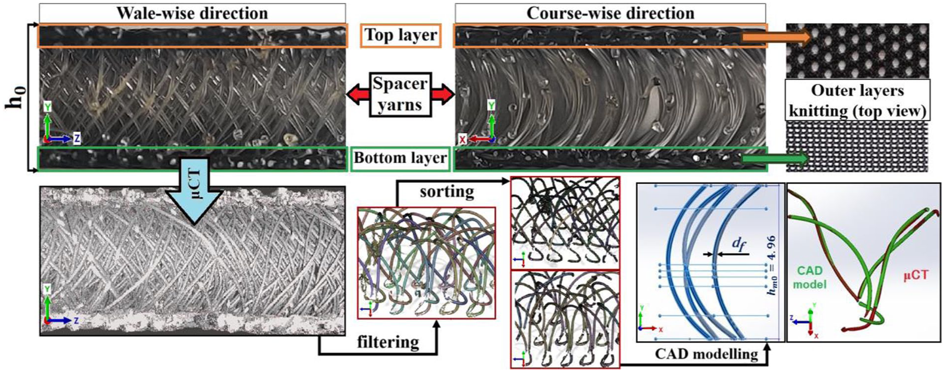
Structure of the 3D WKSF and the procedure for obtaining the 3D CAD of the representative cell.
In light of these assumptions, an important task was to understand the knitting of the middle layer. Visually analyzing the filtered μCT scan, a pattern of the loops could be observed, repeated each two courses (rows). After separating the middle layer, depending on the matching row, it was remarked that the loops that belonged to the same course, and consequently the corresponding yarns, had similar positions and shapes (Figure 1). Thus, in order to reduce the middle layer to a representative unit cell, using the lowest possible number of yarns, two loops (and implicitly, the four yarns) knitted together in two consecutive courses were selected.
The steps taken to reduce the complex structure of the middle layer to four yarns, used for building the 3D model in a computer-aided design (CAD) environment (SolidWorks), are shown in Figure 1, and were presented in detail in Lupu et al. 17 Overlaying the CAD model on the original scanned data of the four selected yarns has shown a good agreement between the two models.
The material of the layers was identified as polyethylene terephthalate (PET), using Fourier-transform infrared spectroscopy (FTIR). Using the traction testing configuration of a rheometer (Anton Paar MCR702 Multidrive) with a dynamic mechanical analysis (DMA) capability, the tensile stress–strain curves for yarns extracted from the middle layer were determined. The experimental data in the linear–elastic zone of the stress–strain curves was curve-fitted to calculate the Young modulus. The averaged value for the Young modulus was determined to be 3.17 GPa (10 trials, standard deviation ±0.27 GPa), which was within the range supplied for PET by the CES EduPack™ database (version 2011, Granta Design Ltd.)
The initial thickness of the 3D spacer and the mean diameter of the yarns were found (using a high-resolution video-microscope and the Videomet software) to be
FEA for behavior during compression
The coordinates of the five-point splines obtained from the 3D CAD model (Figure 1) were used to reconstruct the four yarns of the periodic representative cell in a CAE environment (Abaqus). In addition, a Python-based macro-code was developed to allow for the variation of any parameter within the FE models.
To build a FE model, the four yarns were repeated (ten times) by a linear pattern in the course-wise and wale-wise directions. A sample from a result of a FE model is given in Figure 2. Simulation results have shown that at least seven repetitions are necessary in the in-plane directions to prevent the occurrence of an “edge effect.” This effect can be described as a lack of interaction between yarns, which would typically contact each other during compression, at the edges of the FE model. The spacing between a group of four yarns, 2 mm in the course-wise and 1.575 mm in the wale-wise direction, was determined statistically, by averaging the distance values between five consecutive wales from four courses. The FE models contain also two shell surfaces (
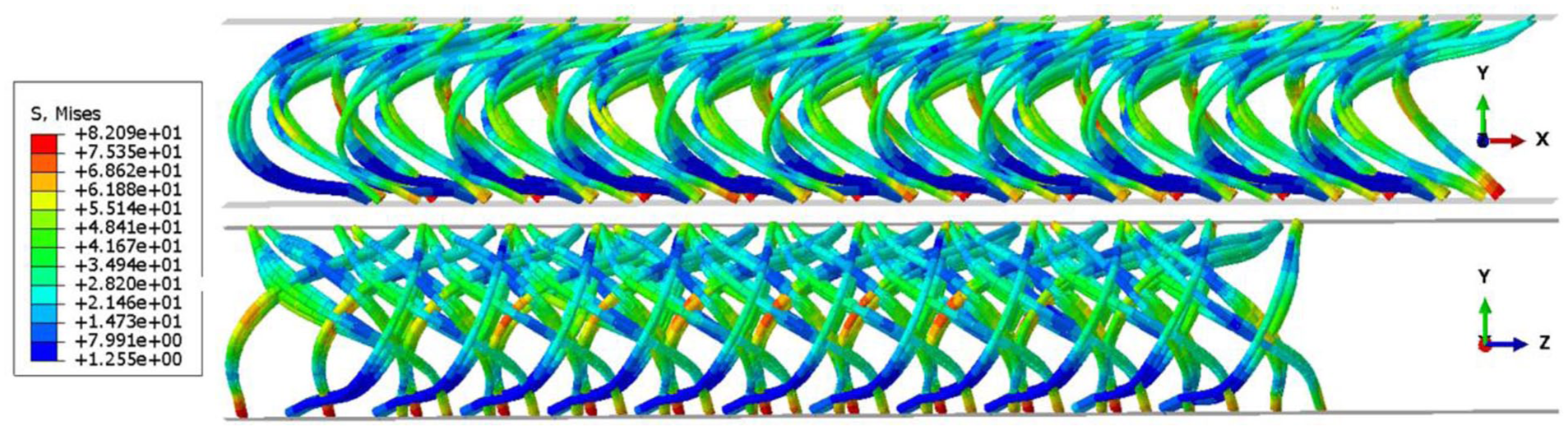
von Mises diagram for T0E1 FE model (strain level
The yarns were meshed using beam elements (type B32) with quadratic interpolation, given the expectation of large rotations and axial strains during compression, and a circular section equal to
The beam nodes located on the plates were separated into two groups, based on the plate they were positioned on. Both groups were fully constrained, displacement and rotation-wise, except for the displacement of the top group in the Oy direction, a condition necessary to allow the compression of the yarns. A similar approach concerning the DOFs offered good results in the preliminary development stages of the FE models presented by Lupu et al.
17
The tie constraint was used to connect these groups of nodes to their corresponding plate (set as master surface). The surface interactions, between yarns and between the yarns and the rigid plates, were modeled using two types of mechanical contact properties: hard contact with separation allowance (normal behavior) and a friction coefficient of 0.2 (tangential behavior).
21
The compression of the yarns was performed using a velocity boundary condition (
The material behavior was assumed isotropic with a bilinear elastoplastic behavior. For the elastic behavior, the experimentally determined Young modulus (
To address the convergence issues of the preliminary models, the numerical simulation software was switched from an implicit/standard method to an explicit one, more suitable for modeling highly nonlinear problems. This improved the simulation of the compression of the yarns, allowing to also reproduce the stage (IV) evolution.
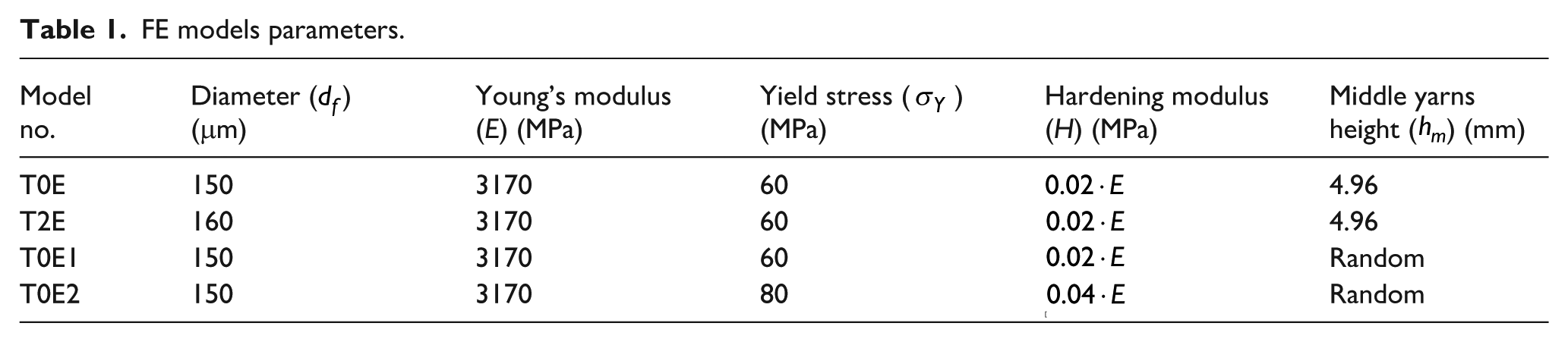
Table 1 presents the main parameters used for the four improved FE models presented in this research. Two models (T0 and T2) from Lupu et al., 17 that have shown promising results in the parametric study, were evaluated with the explicit method. These models use the two mean values determined for the diameter of the middle yarns (obtained with SEM and Videomet, respectively).
FE models parameters.
In Figure 3 one can observe that the results for the T2 and T2E models (“E” stands for explicit analysis) are overlapped until the stopping point of convergence for the T2 model. For the T2E model, the calculation continues until
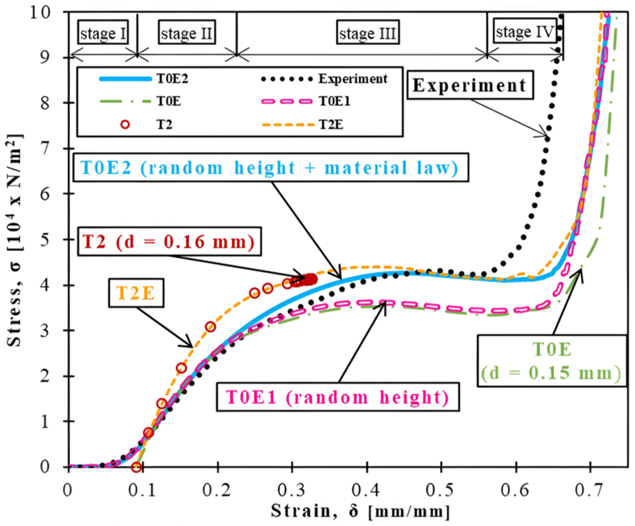
Comparison between experimental and numerical stress–strain curves.
With regards to stage (IV), in both models (T0E and T2E), densification occurs at a higher strain than in the experimental curve. This might be due to the initial height of the yarns in the FE models, as the top and bottom parts touch at a later moment than in reality, a direct consequence of the decision to eliminate the outer layers from the FE analysis. This observation is also sustained by the results obtained with model T2E. Because the yarn diameter of this model has a higher value than that of model T0E, the contact between the yarns endings is initiated earlier, leading to the occurrence of the densification at a lower strain.
To assess the assumption for the initial stage, a randomize command was introduced in the Abaqus macro to vary the initial height of the yarns (
Analyzing the results obtained with T0E1 and T0E2 models (Figure 3) one can observe the appearance of the initial stage for both models, confirming the proposed assumption. For both models having yarns with randomized initial height, stage (IV) is closer to T2E (with the higher value of the diameter). The behavior of the T0E2 FE model, with the modified material law for yarn deformation, closely matches that of the analyzed 3D-WKSF: the first three stages of the numerical and experimental stress–strain curves almost overlap.
Transfer of the deformed yarns to the CFD environment
Despite showing reliable results for the compression behavior, the models with randomized values of the initial height could not be used for the flow analysis. This would have implied importing the entire structure in a CFD environment, which would have resulted in a substantial increase in the computational cost. As the entire approach used to characterize the permeability of the 3D-WKSF was under preliminary evaluation, a tradeoff was made. For the flow analysis through the porous material, the use of the models obtained with the representative cell were preferred, as the entire analysis can be reduced to the study of only four yarns. For this purpose, model T0E was chosen for continuation. However, the other models can be equally considered for evaluation: to identify which model is more realistic.
Using Abaqus postprocessing module, the shape of the yarns at different deformation levels was extracted, with an increment of 0.5–1 mm below
Using another internal developed macrocode, the new files (the .dat files) were imported in SolidWorks. Here, the “negative” of the yarns was extracted through a Boolean operation, using a volume built from a profile identical to the base of the cell (a
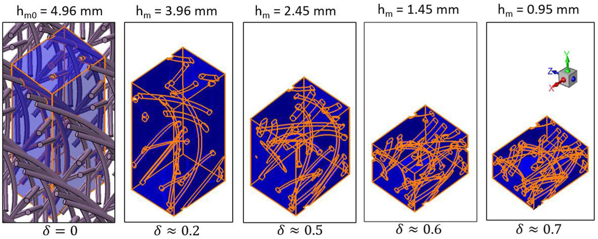
Reduction of the porous volume of the representative cell at different strain levels.
Permeability analysis
Flow models
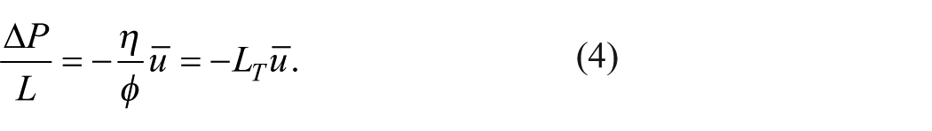
When analyzing the permeability of porous materials, the theoretical model of Darcy 22 is widely used:
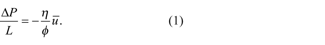
Here,
In the literature, there is a lot of information stating that the Darcy flow regime enters into a transition regime when the pore-based Reynolds number (Rep) value is between 1 and 10.23-25 However, Wang et al.
26
have performed a detailed bibliographic analysis of literature regarding the applicability of Darcy’s law as well as experimental investigation on the lower limit of Darcy regime that demonstrated that the breakdown of this law occurs even at low Reynolds numbers (
The
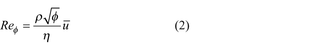
The characteristic length in Equation (2) is permeability,
After the upper limit of the Darcy regime is exceeded, it has been shown that the fluid flow evolves gradually to a steady nonlinear laminar flow.25,32 Among the first to propose an extension of the Darcy theoretical model, to consider the nonlinear behavior, were Dupuit 33 and Forchheimer. 34 The quadratic term added in Equation (1) accounts for the inertia effect in the laminar flow regime. According to Nield and Bejan, 35 the most appropriate extension of the Darcy model is the form proposed by Joseph et al. 36 :
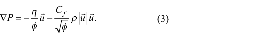
The ratio
Flow analysis
Using the above observations, a CFD model was developed using the volumes extracted from the FE model (Figure 4) in a two steps approach. The first step implied analyzing the fluid flow through the periodic representative cell in the uncompressed state. A pressure gradient was imposed in the wale-wise direction of the 3D WKSF, and the average filter velocity was evaluated from the calculated volumetric flow rate. The numerically obtained data were fitted to the theoretical Darcy model, using the linear regression method, or the Darcy–Forchheimer model, using the least squares method (LSM), similar to the procedure used by Antohe et al. 39 or Boomsma and Poulikakos 30 for aluminum foam blocks. By gradually increasing the pressure gradient it was possible to determine the permeability from the linear flow regime and the quadratic regime parameters to put in evidence the transition to nonlinear flow regime.
The second step focused on studying the periodic representative cell of the material at different compression levels and reduced flow velocities, to obtain the in-plane permeability of the material and its variation with porosity. To remain in the Darcy regime, a reduced pressure gradient was applied, successively, in both in-plane directions to verify the anisotropy of the material as well. With the two results, a resultant permeability was calculated, using a relationship for the summation of the two in-plane permeability components (based on the theoretical model of Gebart 40 in an orthogonal arrangement 41 ). Thereafter, the numerical results were compared with the experimental results obtained by Enescu et al. 20 on the same material.
CFD model description
For each STEP file, be it in its initial, undeformed state or corresponding to a certain strain level (as exemplified in Figure 4), a CFD analysis was performed using the Ansys Workbench suite. In the first step only the wale-wise direction was analyzed (as in Figure 5). In the second step, the flow analysis was performed in-plane, successively on two directions:
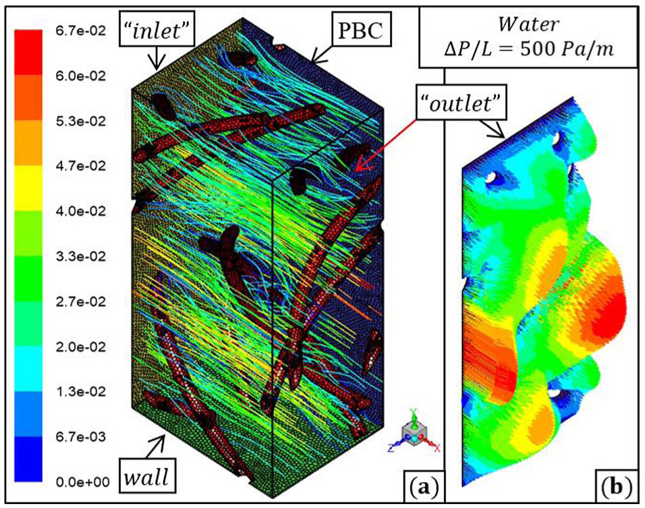
Results from the CFD simulations: (a) velocity streamlines and (b) velocity vector on the “outlet” surface.
To obtain a solution, each CFD model involves resolving some intermediary steps, specific to the chosen module. For this study Fluent module was used. As the geometries imported in the model were complex, all models were meshed with 3D unstructured tetrahedral elements. This allowed us to convert, in the model setup, the initial mesh into polyhedral elements. The number of elements varied between 262,508 (and 1,379,968 nodes) for the uncompressed case to 153,397 (769,577 nodes) for the case with the highest strain level.
The viscous model used in the CFD 3D models was the laminar model. In terms of boundary conditions, the four surfaces on the wale-wise and course-wise directions were defined as mesh interfaces. This allowed the use of translational periodic boundary conditions (PBCs), on the opposite surfaces from the course-wise, respectively wale-wise direction. This boundary condition is useful to join numerically adjacent representative cells (similar to an axisymmetric condition, but of infinite length). When using translationally periodic boundaries, a pressure drop occurs and the flow becomes “fully developed” or “streamwise-periodic.” 42
The offsets of the translationally periodic boundaries were automatically computed to the lengths of the model in the respective direction. The flow between the “inlet” and “outlet,” named this way only to indicate the flow direction, was simulated by imposing a negative pressure gradient in one direction. A stationary wall with a no-slip shear was set as the boundary condition for the opposite surfaces on the
The numerical model was solved using a pseudotransient algorithm for the pressure-velocity coupling. For the spatial discretization of gradients, a least squares cell-based scheme was used. The pressure interpolation was solved with a second-order scheme, whereas for the momentum, a second-order upwind scheme was preferred. The study was performed on a powerful workstation (equipped with an AMD Ryzen processor with 64 cores and 256 GB of RAM).
A mesh-independent solution was sought, for the model using the uncompressed representative cell, in order to analyze the mesh influence over the results. Thus, the total number of elements was varied by limiting the maximum size to 0.05 mm for the coarse mesh (600,471 elements converted into 184,359 polyhedra with 770,475 nodes), 0.035 mm for the medium mesh (1,226,675 elements converted into 262,508 polyhedra with 1,379,968 nodes), and 0.025 mm for the fine mesh (2,667,022 elements converted into 497,989 polyhedra with 2,853,124 nodes). The study was conducted at a reduced pressure gradient (
After reaching the imposed level of residual convergence and calculating a solution, the volumetric flow rate was determined by integrating the velocity component corresponding to the analyzed flow direction over the “outlet” surface. The average filter velocity
Linear flow regime
As stated earlier, the Darcy theoretical model can be used to determine the permeability of a porous medium. According to the literature review, for accurate results the pressure gradients must be restricted to lower values. Equation (1) was rewritten in the form:
The linear coefficient (annotated
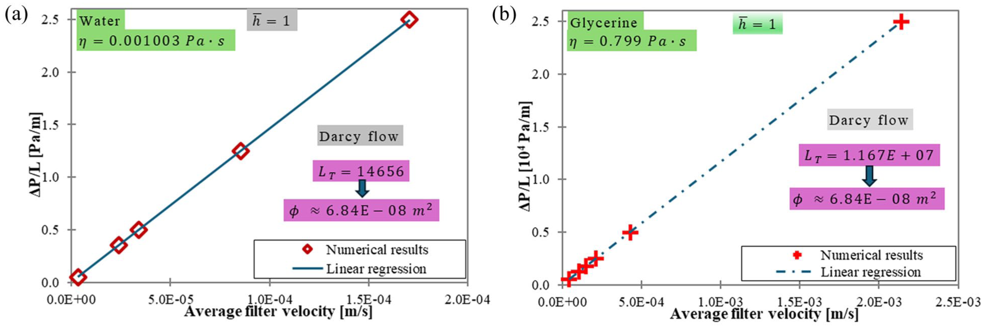
Average filter velocity variation with pressure gradient: (a) water and (b) glycerine, linear flow.
Viscosity has instead a direct influence on the fluid velocity, as higher pressure gradients were necessary in the case of glycerine to obtain velocities closer to those registered with water. The numerical data analyzed in this section showed good correlation with the Darcy theoretical model.
Quadratic flow regime
As the pressure gradient is increased further, the deviation from the linear flow becomes evident. The Forchheimer extension of the Darcy model was investigated to fit the curves and to determine the new permeability. The same approach used for equation (4) was applied to rewrite Equation (3) in the equivalent form:

The quadratic coefficient (annotated
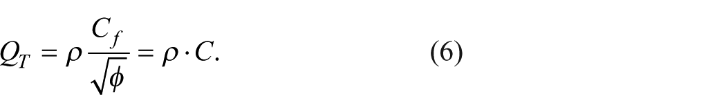
From Equation (5),
(A) Constant permeability:
(B) LSM on all data:
(C) LSM point-by-point
39
:
Two statistical parameters are used to evaluate these methods, the mean deviation of the pressure difference (
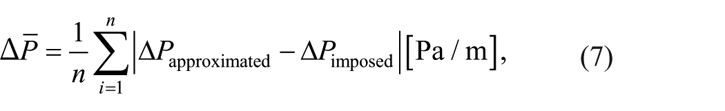
and mean deviation error (
For a good fitting of the numerical data points,
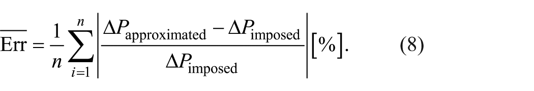
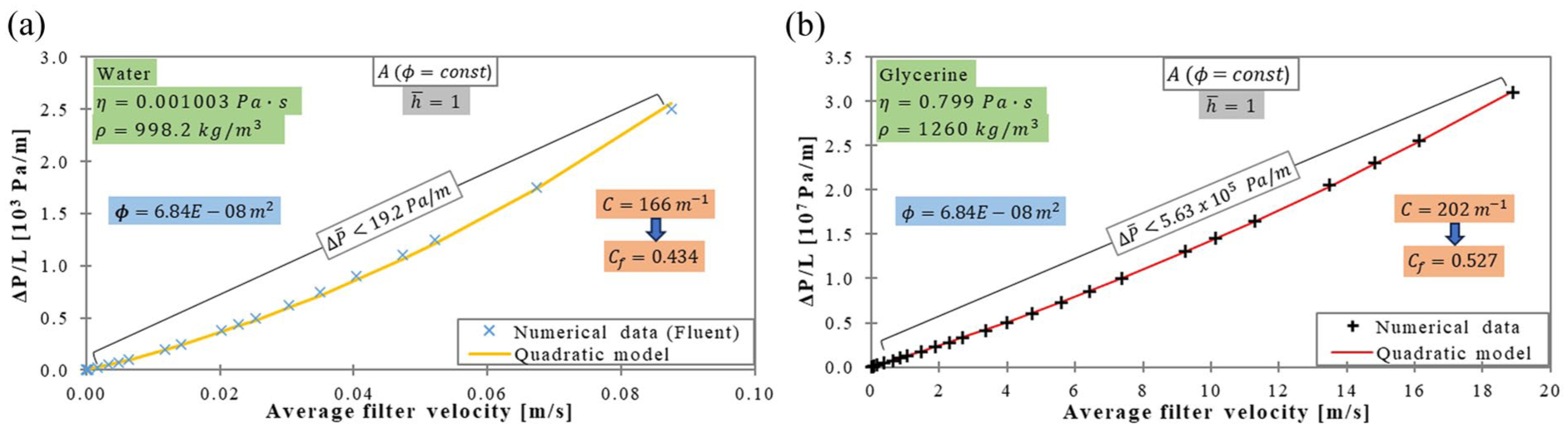
Figures 7(a) and (b) show the results obtained with water and glycerine, respectively, when using method A. The calculated values resulting from the two diagrams, for the viscous and inertial parameters, are summarized in Table 2. With method A, permeability has a constant value, valid for the entire dataset. In addition, the Forchheimer coefficient will behave as a constant and will be estimated from the points in the quadratic flow. This method offered satisfactory results, i.e., the curve fitting the numerical data obtained with water showed a deviation
Average filter velocity variation with pressure gradient for (a) water and (b) glycerine, quadratic flow, method A.
Parameters of the regression curves fitting the full set of numerical data for the two fluids, methods A and B.
From Table 2 (method A), one can observe that
In principle, methods A and B are similar, meaning that both methods will lead to a constant permeability, but the inertia coefficient obtained with method B will be valid for the entire range of data (for both linear and quadratic regime). As explained previously, the two terms of the quadratic regime were approximated with the LSM. With this method, the viscous coefficient value will modify together with the inertia coefficient to obtain the best curve fitting of the data points. The results obtained with method B are also summarized in Table 2.
For glycerine, method B improves the approximation of the numerical data. While for the permeability, the form (
For water, the results were less favorable, as the permeability, form, and Forchheimer coefficients, had diminished values (with 11–
Permeability and inertia coefficient variation with flow regime
As already briefly explained, method C also uses LSM to determine the linear and quadratic coefficients but following a different procedure. The initial values of
The results obtained with this approach led to a good approximation of the curves for both fluids. For water,
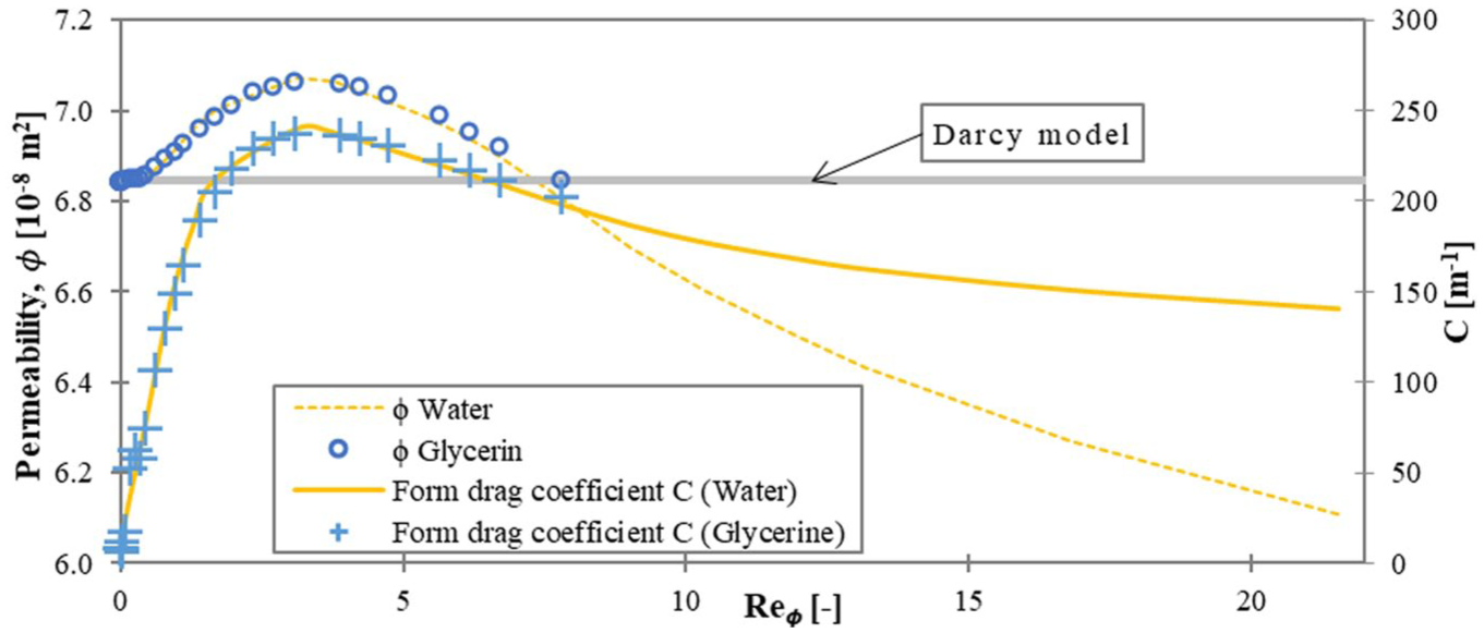
Quadratic model parameters variation with the flow regime (method C).
Analyzing Figure 8, one can observe that the two components of the quadratic theoretical model show similar evolutions with the flow regime, but with different slopes. While in the linear flow regime permeability evolution with
Separation between linear and quadratic flow.
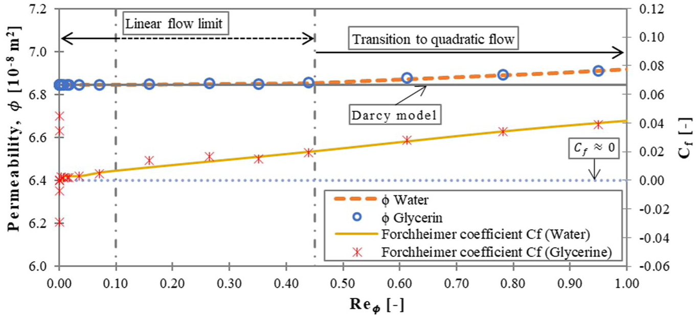
To analyze the behavior in the lower limit of the Darcy flow, the domain was restrained to
From these observations, the assumption is that the “pure” Darcy flow limit for the analyzed 3D WKSF is around
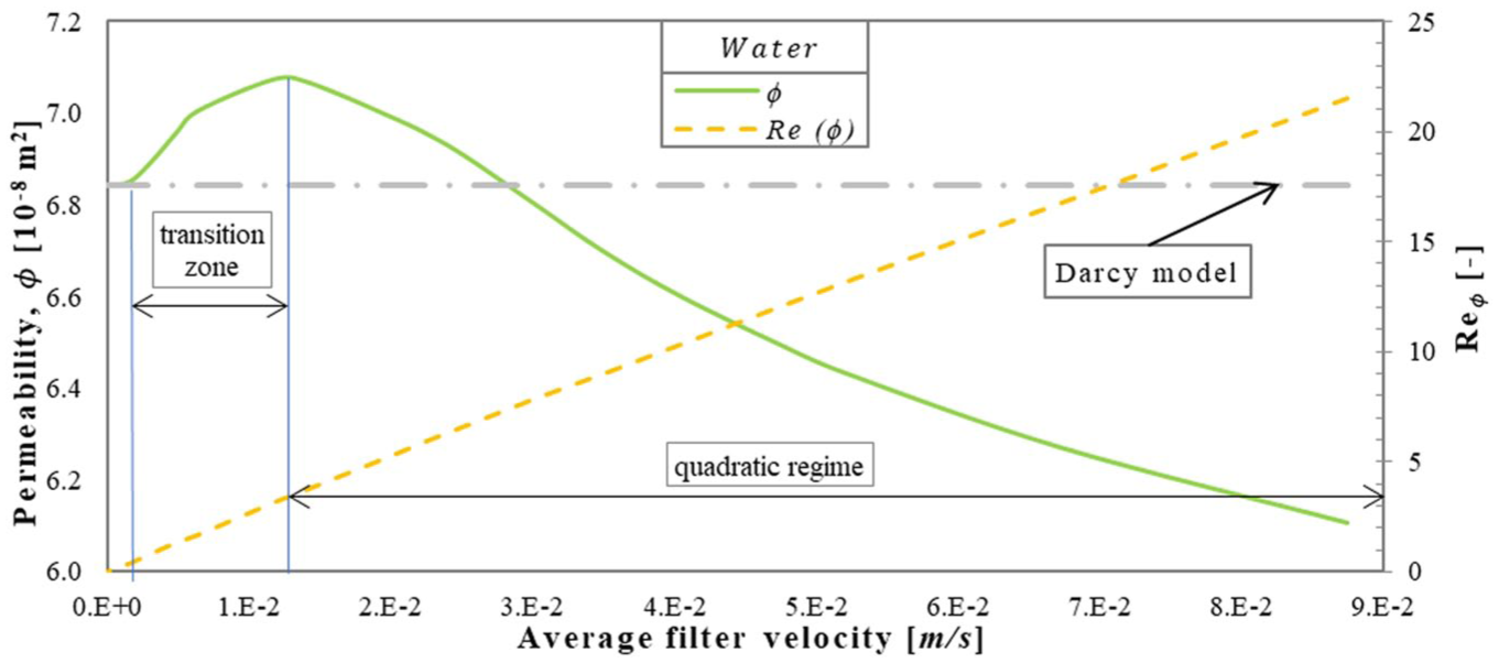
After analyzing the evolution of permeability with the average filter velocity (Figure 10), the end of the transition region (upper limit of Darcy flow regime) was considered to be around the value of
Transition to fully quadratic flow.
This value was found to be close to the limit identified in the numerical study by Fourar et al.
32
In this study the fluid flow through a periodic 3D porous medium was also analyzed, and the conclusion was that the Forchheimer extension of Darcy’s theoretical model fitted the numerical data very well, above the value of
Considering all the observations made in this section in which the permeability of the undeformed 3D WKSF was analyzed, one can say that the quadratic theoretical model fits very well the numerically obtained data, especially when using the approach described in method C. Furthermore, the graphical evolution of the permeability with
Permeability variation with porosity and comparison with experimental data
Extensive experimental activities were performed to evaluate the in-plane permeability of the 3D-WKSF analyzed in this study, with glycerine, on an axisymmetric radial permeameter. With this experimental device, the permeability of this material was experimentally evaluated only for compression rates greater than 40%. 20
It has been shown earlier that, at low velocities, the Darcy theoretical model can successfully be used to evaluate the permeability of the porous medium. To ensure that the flow regime remains within the linear range, a reduced pressure gradient (5000
The Abaqus model used to extract the deformed shapes of the yarns was that identified with T0E. The initial porosity of the 3D-WKSF was evaluated using a CAD software and was determined from the ratio between void volume (Figure 4) and the total volume of the representative cell. The porosity (

Equation (9) was applied only for the middle layer and was considered to yield an “ideal” value. In reality, porosity may vary locally as the position of the yarns can change quite easily. In addition, the outer layers contribute to the reduction of this value, when porosity is evaluated through experimental means, but an evaluation solely of the middle layer would be impossible.
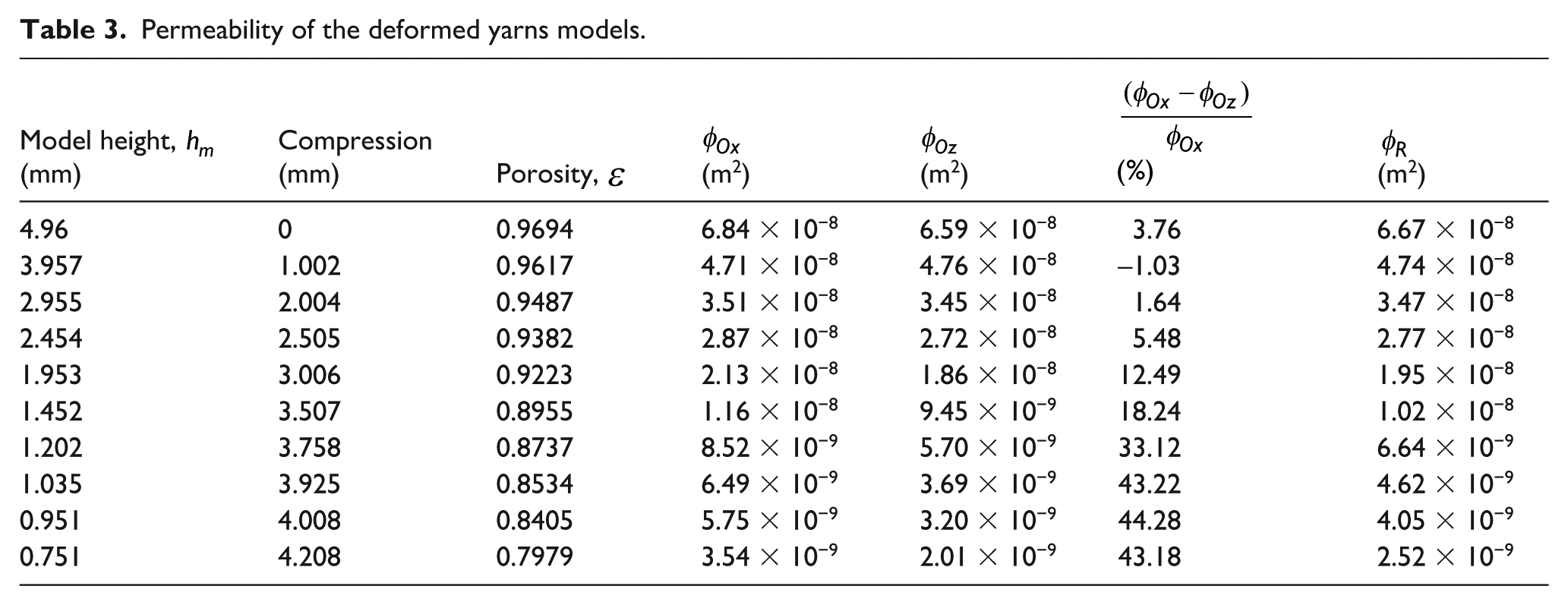
Between the initially undeformed state and the final position when the yarns are fully compressed, a total of eight intermediate positions were analyzed. In the final stages of compression, as porosity reduces, the models were extracted closer to each other. Table 3 presents the values of permeability at different deformation levels of the yarns, in both in-plane directions. At low compressions, the differences between in-plane permeabilities are reduced. As the material is further compressed, the course-wise permeability starts to diminish with 30–45% when compared with the wale-wise permeability. The explanation for this behavior can be related to the way the yarns are deforming. In this sense, at higher compression levels, in the wale-wise direction, the fluid flows along the yarns. In the course-wise direction, the fluid flow encounters increased resistance, as the yarns tend to become perpendicular to the flow. Using this remark, a resultant permeability (
Permeability of the deformed yarns models.
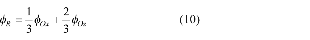
Comparison between numerical and experimental determined permeability for the 3D-WKSF.
Conclusions
An alternative method for the lengthy experimental process of in-plane permeability evaluation of 3D WKSFs has been proposed. The main contributions of the current work included the development of a procedure to obtain a 3D model from scanned images, the simulation of the force–deformation behavior using FEM, and the coupling of this mechanical simulation with the fluid flow analysis.
The novelty consisted in establishing a correlation between force and deformation over a wide compression range, extending close to the densification phase, as well as determining the in-plane permeability through CFD simulation, validated by experimental results.
This method was developed reducing a μCT scan of the material to a representative cell comprising only four yarns. Using the concept of a periodic representative cell of the middle layer offers reliable results, in terms of the and compression stages II and III of the deformation mechanism. The compression stages I and IV depend more on the position in the outer layers of the yarn endings, which were eliminated in the process of obtaining the unit cell. Nonetheless, the randomizing function in the macrocode used to generate the 3D FE models in Abaqus has put in evidence also the compression stage (I), which was missing initially from the improved FE models. Moreover, the deformation mechanism of the yarns was well described with the bilinear elastoplastic model.
The CFD analysis gives reliable results when evaluating the permeability of the material. The numerically obtained data have been evaluated using the Darcy–Forchheimer theoretical model. At low velocities, the permeability is constant and independent of the fluid properties. At higher velocities, the viscous and the inertia coefficients vary with the pressure gradient and act simultaneously to reduce the fluid flow velocity. Using the LSM and a point-by-point approach to fit the curve obtained from the numerical results, the limit between different flow regimes was analyzed.
The numerically predicted data are also in good agreement with the experimentally determined permeability, obtained in similar flow conditions. Based on these results, one can conclude that the influence of the outer layers on the fluid flow is not particularly important in laminar conditions and when applying reduced pressure gradients. Thus, the permeability of the 3D WKSFs can be considered that of the middle layer, as long as the two surface layers do not contact each other.
The methodology described in this study can be successfully applied to evaluate the variation of permeability with porosity for a 3D WKSF subjected to compression. In addition, when developing user-defined 3D WKSF structures, the method presented herein can be very useful in reducing the overall expenses for prototyping and testing.
The findings of the present study also align with the previous research on compression behavior and permeability of 3D textiles. Just as in the approach of Liu and Hu, 15 a unit cell approach was used, but with a simplified four-yarn structure, improving computational efficiency. While earlier studies13,15,16 struggled also to capture the plateau and densification stages, the current solution had an enhanced accuracy, except also for the densification stage, which appeared at a higher strain, although correctly predicted in terms of stress. In contrast to Orlik et al. 18 whose permeability predictions showed similar discrepancies and had only one numerical predicted value, the present approach successfully coupled CFD and FEA, validating numerical results with experiments.
Future work should focus on improving, automating, and optimizing various aspects of the procedure to enhance its accuracy and efficiency. Although some simplifications and compromises were necessary, the findings provide a strong starting point for improving how permeability is evaluated.
Footnotes
Acknowledgements
The authors wish to express their sincere gratitude to Mr. Florin Pisică and Mr. Florin Samoilă from Top Metrology (Romania) for their generous contribution of a professional 3D scan of the spacer fabric, which enhanced the value of this work.
Declaration of conflicting interests
The authors declared no potential conflicts of interest with respect to the research, authorship, and/or publication of this article.
Funding
The authors disclosed receipt of the following financial support for the research, authorship, and/or publication of this article: The authors gratefully acknowledge the financial support provided by the French National Research Agency to conduct the ANR project 19-CE05-0005, entitled “Saturated open-cell Foams for Innovative Tribology in Turbomachinery – SOFITT.”