Sage Journals: Discover world-class research

Abstract

Cotton fiber length is one of the most critical parameters of fiber quality for ring-spun and air-jet-spun yarns. Currently, two of the most common instruments for testing cotton fiber length are the USTER High Volume Instrument (HVI) and the USTER Advanced Fiber Information System (AFIS). The HVI bases its length measurement on the fibrogram concept. It is fast but reports only two length measurements—the upper half mean length (UHML) and the uniformity index (UI), where the UI is the percentage ratio of mean length (ML) to UHML. The AFIS is slower and more costly per test because it individualizes fibers to provide a complete fiber length distribution per sample. This paper presents a method that can reconstruct a complete fiber length distribution from an HVI fibrogram based on established fibrogram theory. Results show that the algorithm can accurately recover different types of distributions based on synthetically generated data. Results also show that reconstructed distributions of three different types of samples—upland, pima, and viscose—differ in ways that make sense based on known characteristics of their length distributions. Finally, a variety of statistics computed from the reconstructed distributions are compared to the HVI-reported length parameters. Results show a good correlation with HVI output with R² ranging from 0.730 to 0.965 across nine different methods of calculating the ML, UHML, and UI. Interestingly, statistics calculated from an approximation of the length distribution by weight are the most closely related to the HVI length parameters.

Keywords

Cotton fibers fiber length distribution High Volume Instrument Advanced Fiber Information System short fibers uniformity

In the cotton industry, the evaluation of cotton fiber quality is of vital importance. Not only does fiber quality determine the selling price of cotton, but it also assists spinners in configuring their equipment. Among fiber properties, one of the most critical factors is fiber length, as longer fibers allow spinners to produce finer yarns, which yield a higher price.^1–4

As cotton is a natural fiber, fiber lengths within a sample can vary widely. As such, several fiber length measurements are used by the cotton industry to attempt to describe the within-sample length variation. For example, the United States Department of Agriculture (USDA) Agricultural Marketing Service (AMS) classes every bale of cotton commercially produced in the USA. Among other fiber properties, the upper half mean length (UHML) and the uniformity index (UI) are provided for each bale by testing one sample from each side of the bale using the USTER High Volume Instrument (HVI) (USTER Technologies, Inc., Knoxville, TN, USA)^5,6 (the UI is the percentage ratio of the mean length (ML) to UHML). Fiber length is also essential to cotton breeders as they select new lines with fiber qualities that meet the current and future demands of the textile industry.^7–9 Along with the HVI, some breeders also test samples with the USTER Advanced Fiber Information System (AFIS), which provides other length measurements, such as the upper quartile length (UQL) and short fiber content (SFC).¹⁰

The HVI and AFIS are two of the most common instruments used to measure cotton fiber length, but their measurement methods are different. The AFIS uses a mechanical opener to individualize fibers from a prepared 0.5 g hand-shaped sliver. Fibers are transported past a sensor that measures fiber length as well as other properties. One of the unique aspects of the AFIS is that it provides a complete fiber length distribution of the sample from which several statistics are computed, for example, the UQL and SFC mentioned above.¹¹ On the other hand, the HVI uses a fibrosampler and comb to prepare a fiber beard from a 10 g sample. To create the fiber beard using the fibrosampler, the sample is placed inside a rotating drum. Inside the drum, mechanical fingers press the sample into the perforated portion of the drum (Figure 1(a)). As the drum rotates, the protruding fibers are caught by the needles of the comb, which are then carded by the back side of the drum as it continues to rotate (Figure 1(b)). The HVI then uses a brush (Figure 1(c)) to parallelize the fibers and remove loose fibers and trash, producing a fiber beard as shown in Figure 1(d). The fiber beard is then inserted between an array of light-emitting diodes (LEDs) and an array of sensors (Figure 1(e)). Figure 1(f) shows a diagram of this scanning method where the point of view is from the side and in the plane of the beard. As the beard passes between the LEDs and sensors, the system records the amount of light attenuated by the beard versus the displacement of the comb, which is meant to estimate the number of fibers blocking the light at the given length or displacement.¹² The resulting attenuated-light-versus-displacement curve is called a fibrogram (Figure 2), from which the HVI calculates the UHML and UI (more details are provided later)

Figure 1.
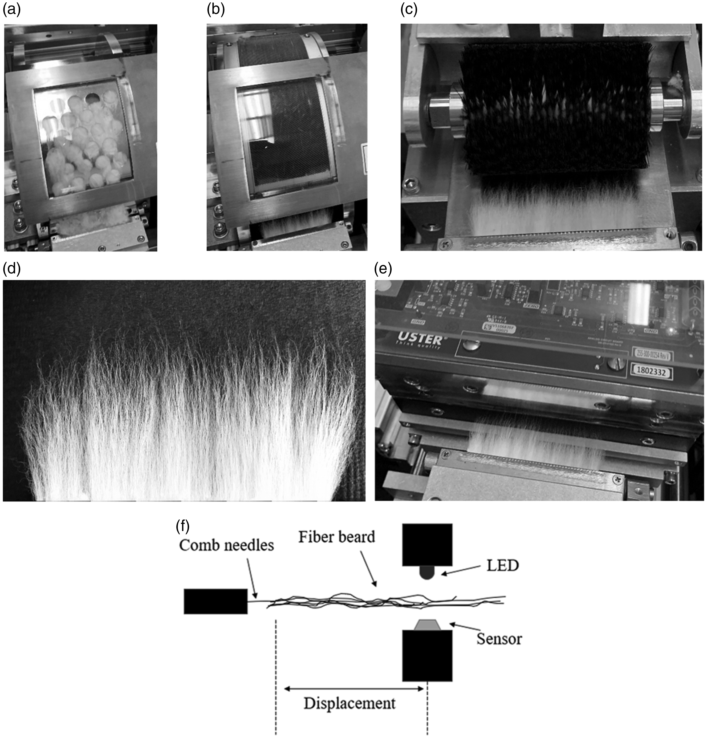
The process of the High Volume Instrument (HVI) length measurement: (a) comb needles (bottom of image) catch fibers protruding through the holes as the drum containing the sample is rotated; (b) the fiber beard (bottom of image) is carded by the back side of the drum as the drum rotates; (c) the fiber beard is brushed; (d) close up of fiber beard after brushing; (e) the fiber beard is inserted into a module containing a row of light-emitting diodes (LEDs) and a row of sensors and (f) diagram showing how the HVI captures the length of the fiber beard. The system records the amount of light attenuated by the fiber beard versus the displacement.

Figure 2.
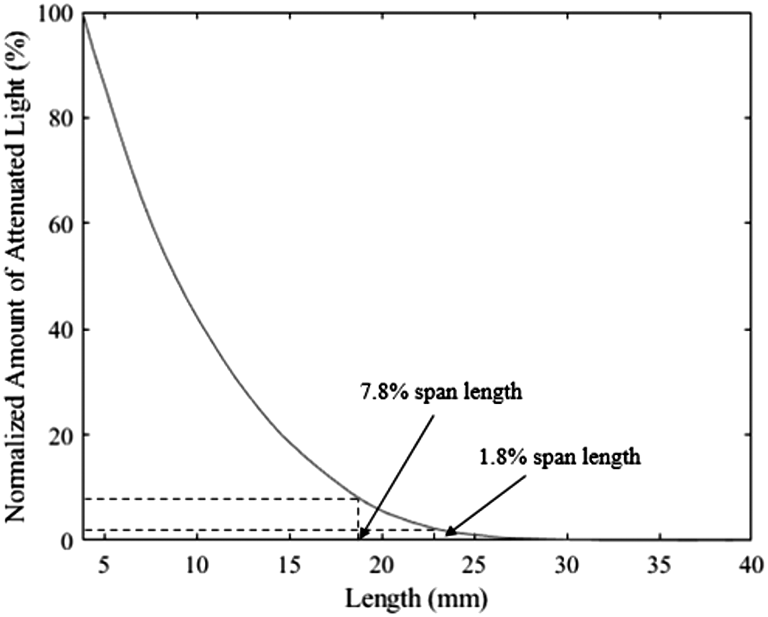
Sample fibrogram. The amount of attenuated light (y-axis) is normalized such that the fibrogram ranges from 0% to 100%. The 7.8% and 1.8% span lengths are highly correlated (R² = 0.99) with the High Volume Instrument measurements of mean length and upper half mean length, respectively.¹³

The differences in the measurement methods between the AFIS and the HVI also create a difference in the total test time with each instrument. The AFIS allows for the selection of 1000–10,000 fibers per test. A typical research protocol calls for five repetitions of 3000 fibers per sample. A single test with the AFIS takes approximately 8 minutes to process 3000 fibers. On the other hand, the HVI conducts a two-repetition test in approximately 30 seconds with the fiber beards generated from each repetition containing approximately 15,000–20,000 fibers.^13,14 While the HVI provides less detailed information, particularly in terms of length, the speed presents a major advantage.¹¹ For the USDA-AMS, the HVI is the only instrument that can efficiently test the 15M+ bales of cotton grown in the USA each year within a 4–5 month time frame following the fall harvest season. Similarly, for cotton breeders, the HVI is the testing method of choice for all but the more promising lines due to budgetary constraints. The increased sample preparation and testing time for the AFIS necessitates that the cost per test is often several times higher than that of the HVI.

As previously mentioned, the HVI bases its length measurements on the fibrogram concept. Recently, there has been some investigation of the fibrogram produced by the HVI to potentially extract additional length parameters. In 2020, Sayeed et al.¹³ demonstrated that the current UHML and ML are highly correlated with the 1.8% and 7.8% span lengths, respectively (R² = 0.99 for both). These two span lengths represent the longest part of the fibrogram, as shown in Figure 2, and were shown to be highly correlated with each other (R² = 0.95). Using the complete fibrogram curve, they used principal component analysis to extract three independent variables from the fibrogram to represent the variation captured by the entire curve and showed that these three variables predict yarn quality better than the current HVI length parameters. Later, Sayeed et al.¹⁵ developed a multivariate correction method to align the fibrogram measurement as a whole curve across multiple HVIs and demonstrated that it is possible to bring the fibrogram measurements at a similar level across many HVIs. Also, Tesema et al.¹⁶ showed that the whole fibrogram curve is stable and repeatable over long- and short-term periods for a single HVI by examining several span lengths along the curve. They also proposed a correction procedure similar to the current HVI calibration procedure that can reduce the differences between HVIs for several span lengths across the whole fibrogram curve. In summary, their work shows that, while the HVI currently only uses and calibrates two points along the curve, the entire curve is stable and correctible across HVIs.

While the work by Sayeed et al.¹³ shows that more length information is contained in the whole fibrogram than that currently provided by the HVI output, the measurements produced by their method, the principal components, exist in a latent space devoid of any statistical interpretation of the length distribution. Similarly, while the current HVI length measurements derived from the fibrogram are called the ML and UHML, it has not been shown how they relate to the length distribution of the fiber beard. In fact, as we show in the following section, the current theoretical interpretation of the fibrogram has no foundation for relating span lengths (lengths at which a horizontal line intersects the fibrogram) to distribution statistics. For example, there is no mathematical, theoretical link between the 7.8% span length and the mean (or any other statistic) calculated from the distribution. Other methods exist that create a fiber length distribution from a dual beard sample, for example, Zhou et al.,¹⁷ but sample preparation and measurement time are much slower than the HVI.

To remedy these issues, we present a new algorithm that reconstructs the fiber length distribution from a HVI fibrogram. The algorithm is based on an extension of fibrogram theory and employs windowed curve-fitting techniques to reconstruct the length distribution as well as the cumulative distribution function (CDF) of the fibers present in the fiber beard. In the following sections, we review fibrogram theory and discuss the details of the new algorithm. We will also show its effectiveness by using synthetic data as well as visually comparing reconstructed distributions of upland, pima, and viscose samples. Finally, we compare statistics computed from reconstructed distributions to the current HVI length parameters for 2498 commercial samples.

A review of fibrogram theory

A seminal work on fibrogram theory is attributed to KL Hertel.¹⁸ In his work, Hertel describes a fiber beard prepared from a sliver and analyzed using a fibrograph. The fibrograph is a device that uses photovoltaic cells to measure the amount of light attenuated by the fibers at various lengths along the fiber beard. As previously mentioned, the amount of light attenuated is considered an approximation of the number of fibers at that length, and the resulting curve is called a fibrogram.

In generating the fiber beard from a sliver, one of the key assumptions Hertel¹⁸ asserts is that “the fiber is to be selected at random and every point on every fiber is equally probable.” Later, Chu and Riley¹⁹ put forth that this assumption by Hertel translates into two key points:
a sampled fiber is held at a random point along its length;

the probability of sampling a particular fiber is proportional to its length.

However, Chu and Riley¹⁹ altered these assumptions as they were establishing the fundamental principles of a fibrogram based on a fiber beard prepared by a fibrosampler:
The mathematic techniques developed by Hertel may be modified for the assumption that every fiber has an equal probability of being caught by the comb needles regardless of its length. The holding point along each sampled fiber length is assumed to be random. Thus, for a monolength fiber sample, the shape of the fibrogram is triangular.¹⁹

Continuing with Chu and Riley’s explanation, given a sample of length L and a total number of fibers N, the fibrogram R measured at a distance x can be written as
$R (x) = N (L - x) / L$
(1)
where R is in units of the number of fibers. Figure 3 shows a graphical representation of this.

Figure 3.
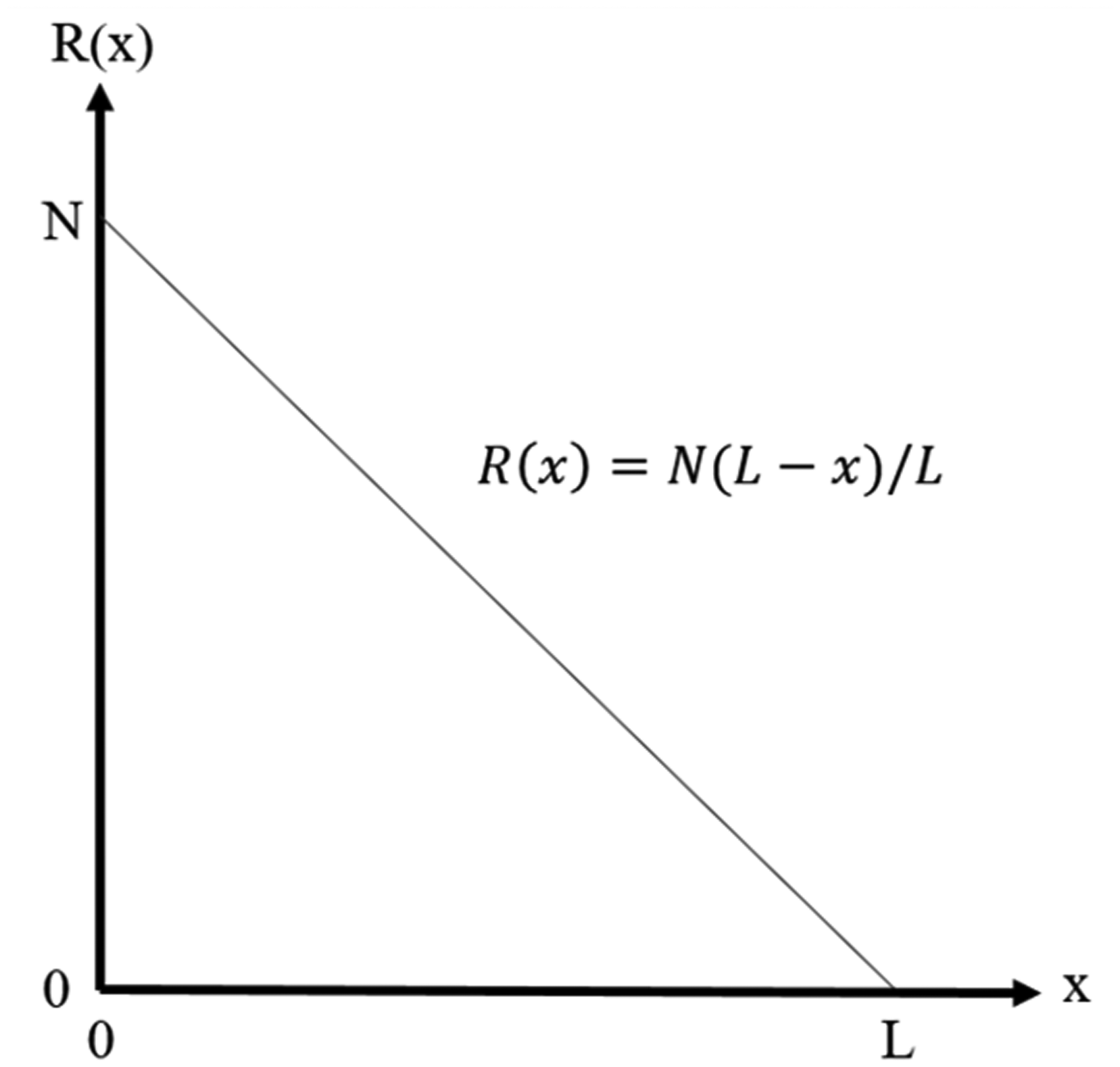
Fibrogram of a monolength fiber sample, where N is the number of fibers and L is the length.

Expanding on equation (1), if instead of a monolength sample, we are given a length frequency distribution of the fiber beard, n(L), the equation for the fibrogram then becomes
$R (x) = \int_{x}^{L_{m}} \frac{(L - x) n (L)}{L} d L$
(2)
where L_m is the length of the longest fibers in the sample. Also note
$R (0) = \int_{0}^{L_{m}} \frac{(L - 0) n (L)}{L} d L = \int_{0}^{L_{m}} n (L) d L = N$
(3)

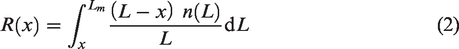
From equation (2), the first and second derivatives of R(x) are as follows
$R^{'} (x) = - \int_{x}^{L_{m}} \frac{n (L)}{L} d L$
(4)

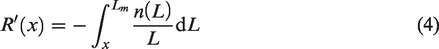
and
$R^{″} (x) = \frac{n (x)}{x}$
(5)

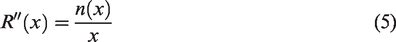
Furthermore, Chu and Riley¹⁹ describe a tangent line on the fibrogram at a distance x, as shown in Figure 4. Using the coordinates of two points along the line, the equation of this line can be written as
$Y (x) = R (x) - x R^{'} (x)$
(6)

Figure 4.
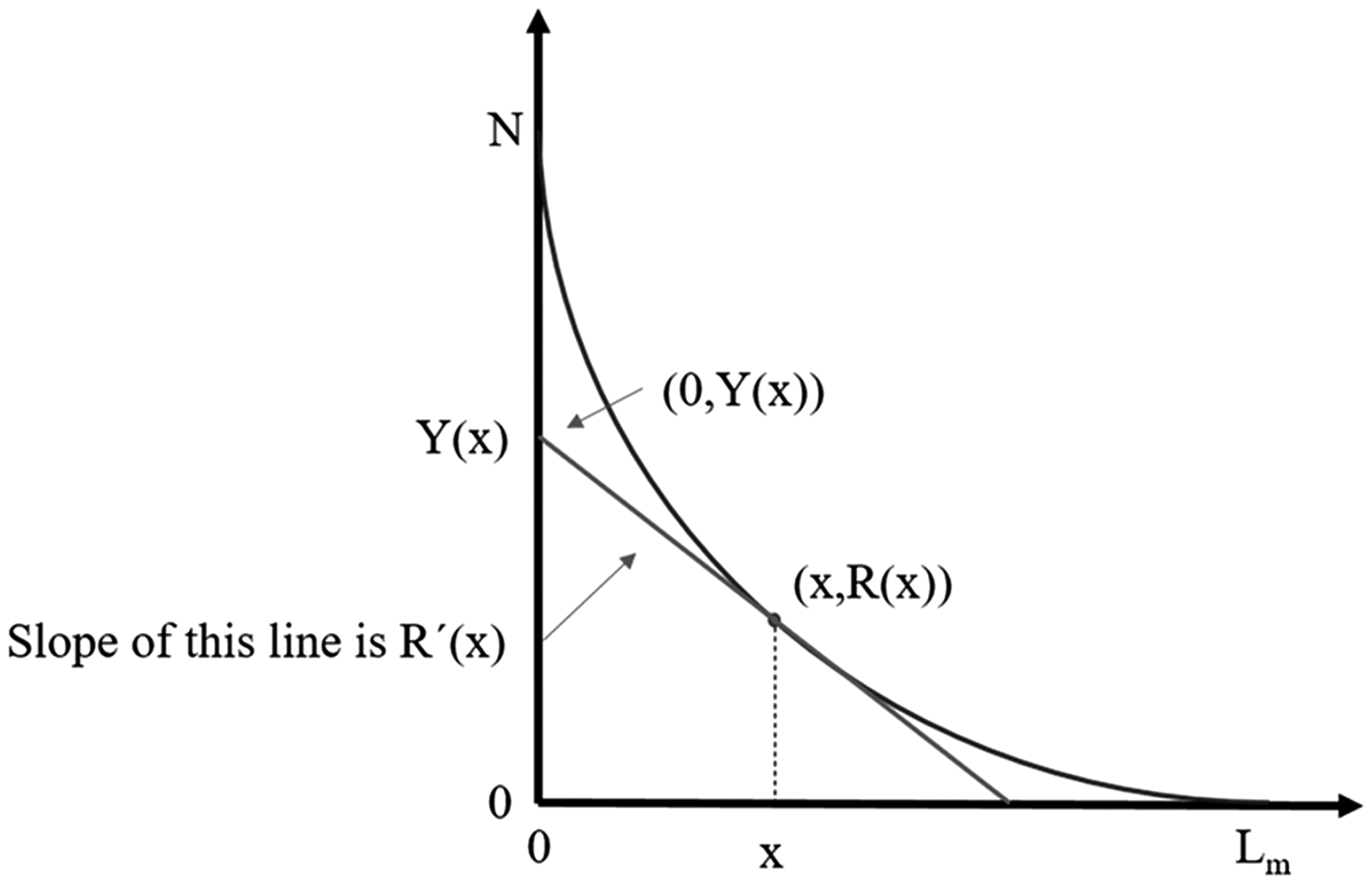
A tangent line to the fibrogram at length x with a y-intercept at $Y (x)$ .

By plugging equations (2) and (4) into equation (6) and solving, we get
$Y (x) = \int_{x}^{L_{m}} n (L) d L$
(7)

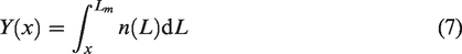
Here we see that $Y (x)$ is a CDF, that is, $Y (x) = P (X \geq x)$ . From equation (7), the distribution, $n (x)$ , can be derived as
$n (x) = - \frac{d Y (x)}{d x}$
(8)

It is important to note that while this theoretical formulation is based on a length–frequency distribution where $n (x)$ provides the number of fibers at length $x$ , $n (x)$ can also be considered to provide the percentage of the number of fibers at a given length without loss of generality. In this case, the sum of the length–frequency distribution and, hence, $R (0)$ , are equal to 100%. This representation relates to the concept of normalizing the amount of attenuated light such that most of the light is blocked (considered as 100% attenuation) when the maximum number of fibers are present at that point on the beard.

Algorithm description

While the formulas above provide a mathematical relationship between the fibrogram and the underlying length distribution, reconstructing the distribution from a fibrogram acquired via some type of sensor system presents a set of problems that must be addressed. This section details the method for reconstructing the length distribution while also addressing some practical issues that arise from a fibrogram produced by the HVI.

Theory versus real world application

One of the most important factors in reconstructing the distribution from fibrograms is the assumption of convexity in the theoretical fibrogram. According to equation (5), since the length distribution, $n (x)$ , is always positive, and we are only interested in positive lengths (i.e. $x > 0$ ), the second derivative of the fibrogram (5) is always positive. Hence, equation (2) is a convex function for $x > 0$ . However, in practice, a fibrogram acquired from a fiber beard may exhibit areas of concavity due to several factors.

Firstly, imperfections in the fiber beard may be caused by small trash particles as well as neps (fiber entanglements), as shown in Figure 5. Other issues could be caused by ineffective carding or brushing, such as fibers not being attached to the comb. In theory, as the beard is scanned from the base to the tips of the fibers, one would not expect the density of the beard to increase. However, these imperfections may cause a perceived increase in fiber density, which would manifest as concavity in the fibrogram.

Figure 5.
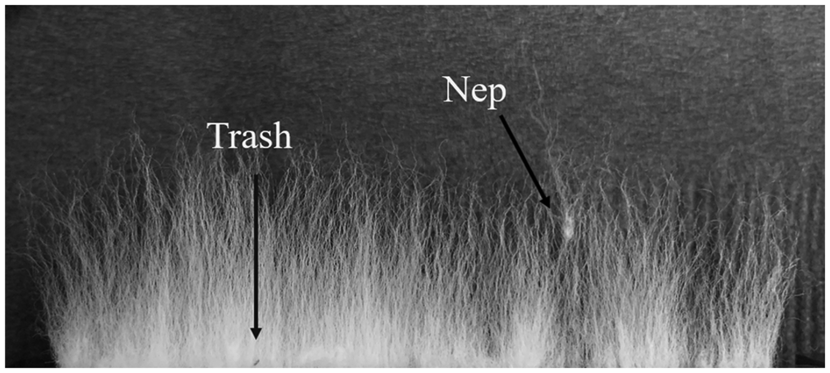
Fiber beard with an example of a nep as well as a trash particle.

Another major source of concavity could be due to the LED light interacting with the comb when it is near the sensors. Perhaps to avoid this issue, the HVI begins scanning the beard 3.81 mm away from the comb.²⁰ However, observationally, the beginning part of the fibrogram output by the HVI frequently exhibits concavity. Figure 6 shows an example of a fibrogram with concave regions shaded. In these regions the second discrete difference of the curve, that is, the second derivative, is less than zero. Note the larger highlighted portion at the beginning of the curve (from 3.81 to ∼6 mm). Concavity in this region appeared very frequently, which led us to hypothesize that close proximity of the comb to the sensors creates interference.

Figure 6.
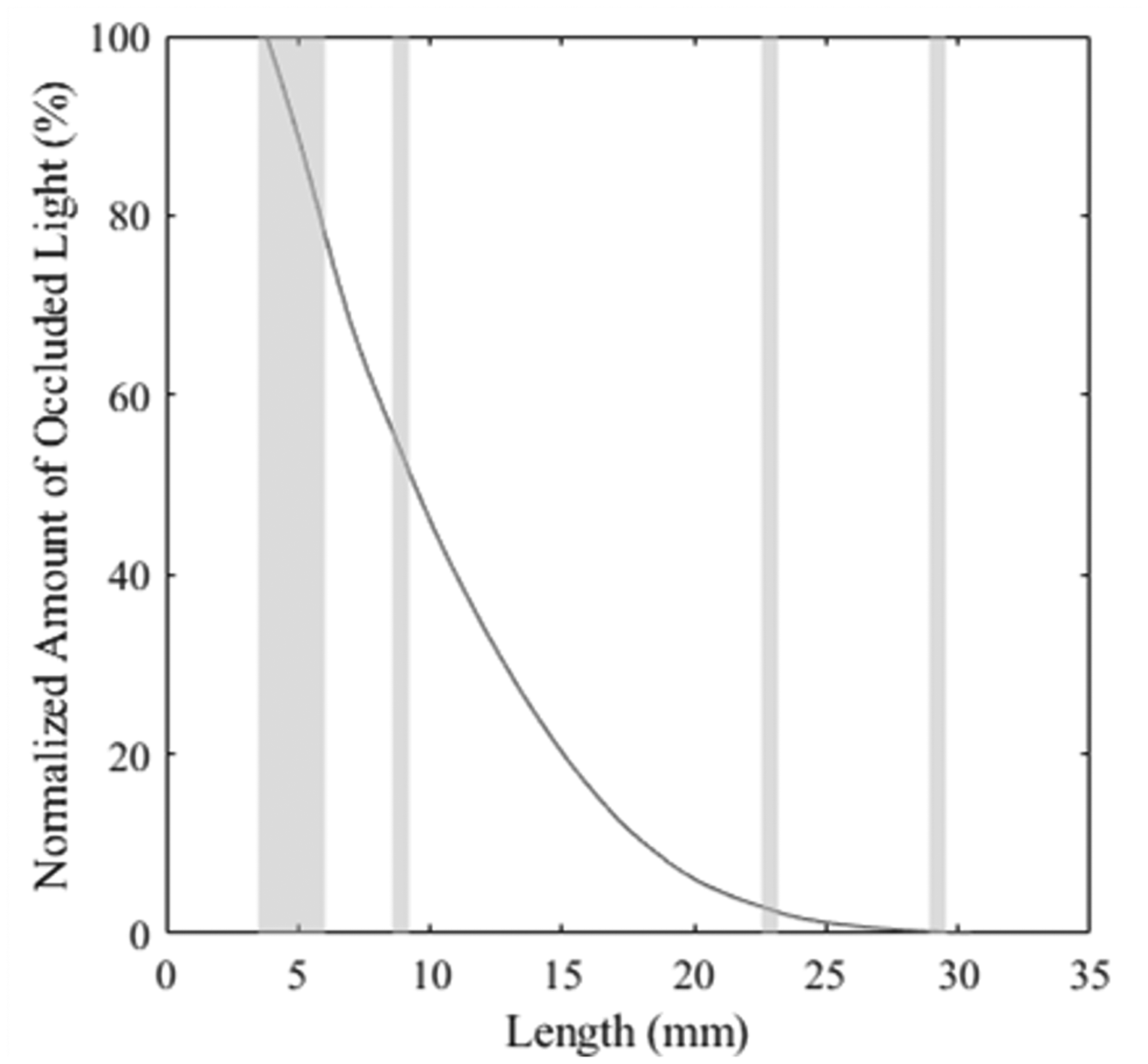
Sample fibrogram with areas of concavity highlighted.

Finally, noise in the sensor can also be a source of concavity. The other smaller concave regions highlighted in Figure 6 could be due to trash or sensor noise.

Noise also becomes an issue when the fibrogram is near zero. Theoretically, the value of the fibrogram should be zero after the longest fiber has been scanned. However, in practice, the scanning mechanism of the instrument does not stop at the tip of the longest fiber and, instead, continues until some fixed length has been reached. For example, the HVI scans the fiber beard from 3.81 to 54.61 mm away from the comb at 81 discrete points with 0.635 mm between each point. The signal-to-noise ratio is low in the region where little to no fibers are available to block the light, rendering the data in this region unreliable. Therefore, the algorithm must determine the approximate length of the longest fibers of the sample and ignore or remove any data beyond that point.

Algorithm details

The proposed algorithm attempts to resolve these practical concerns in three ways. Firstly, it determines the end of the fibrogram—that is, the point at which the longest fibers have been scanned after which the remaining data is assumed to be zero. Secondly, it reconstructs the initial, missing portion of the fibrogram (0–3.81 mm) as well as the initial portion of the curve likely affected by the comb based on a convex function. Finally, it applies a windowed curve-fitting procedure, which smooths the curve, removing any slightly concave portions while also providing a way to estimate the fibrogram equation and its derivatives.

Furthermore, the algorithm details below present a general approach that could be applied to a fibrogram acquired from a sensing method similar, although not necessarily identical to the HVI. The Experimental methods section discusses more specific parameters that were used in processing the HVI fibrograms in these experiments.

Determining the end of the fibrogram

The end of the fibrogram is determined when one of two conditions is met (whichever comes first):
the value of the fibrogram is zero;

the first derivative (i.e. first discrete difference) of the fibrogram is greater than or equal to zero.

The first condition is obvious since, in theory, the fibrogram reaches zero at the length of the longest fiber in the sample. The second condition also comes from the derivation of the fibrogram equation, but serves a more practical purpose. In equation (4), we can see that $R^{'} (x) < 0$ for $0 < x < L_{m}$ and $R^{'} (L_{m}) = 0$ . In other words, the first derivative is negative over the entire domain except for the longest fiber, $L_{m}$ , at which point it becomes zero. In practice, the region of the curve with the longest fibers becomes noisy and, in some cases, the first derivative (i.e. first discrete difference) may become positive due to noise before the fibrogram reaches zero. In that case, we can conclude the noise is greater than any signal produced by the instrument and, therefore, the data to the right of that point cannot be trusted. As such, that point and all data to the right, ${x \geq L}_{m}$ , are simply discarded.

As an example, consider the two fibrograms in Figure 7 from the same cotton sample. Each of these graphs is zoomed into a portion of the fibrogram curve as it nears zero between 25 and 50 mm. Note that the percent of attenuated light (y-axis) is 1% or less. Also, in these graphs we have included the discrete points of the fibrogram, indicated with small circles. In Figure 7(a), the fibrogram reaches 0% attenuated light near 31 mm. To the right of that point, it appears that noise in the signal causes the fibrogram curve to fluctuate, making the data unreliable. In this case, the algorithm would end the fibrogram at 31 mm following Condition 1 above. On the other hand, in Figure 7(b), the fibrogram does not reach 0% attenuated light until ∼35 mm; however, the fibrogram slightly levels off at 30 mm and after that appears noisy. Following Condition 2, the algorithm would end the fibrogram at 30 mm, after which point the derivative becomes 0.

Figure 7.
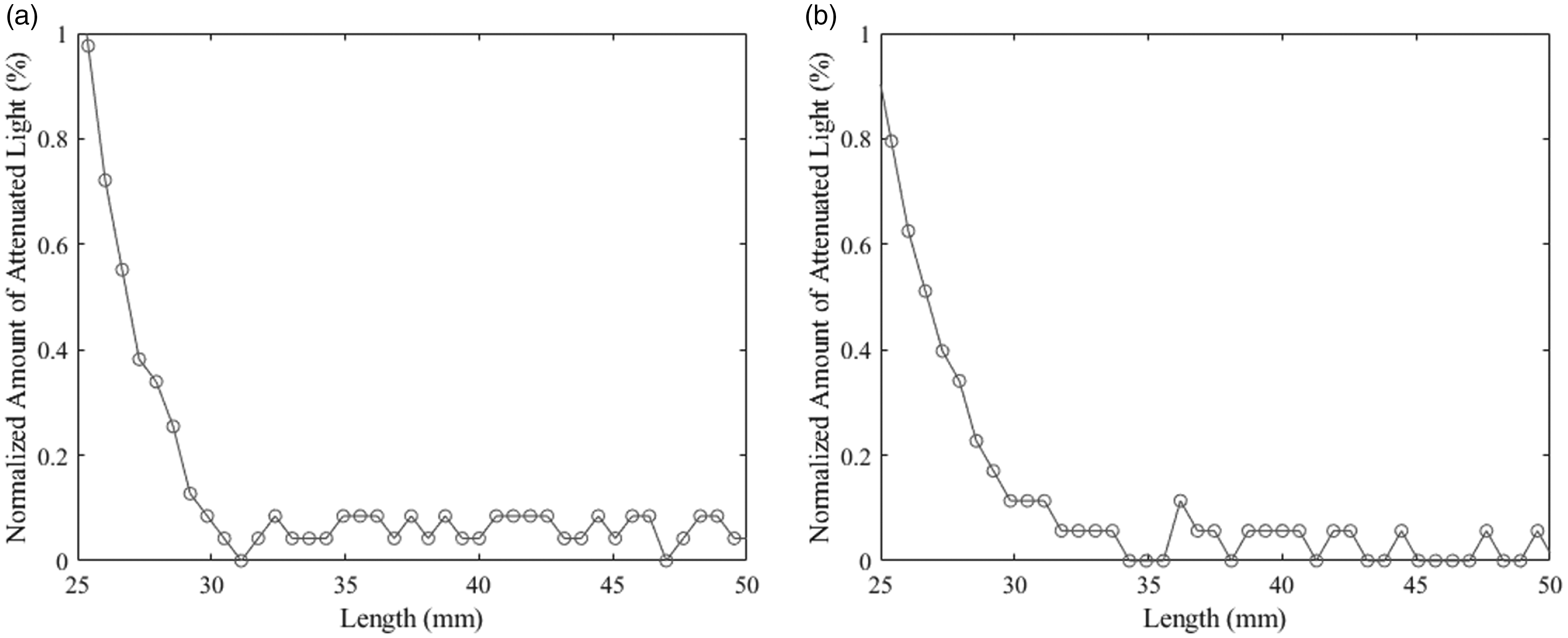
A close-up view of the end of two fibrograms where the noise is present near 0% light attenuation: (a) Condition 1 triggers at 31 mm and (b) Condition 2 triggers at 30 mm.

Estimating the beginning of the fibrogram

The initial part of the fibrogram can be estimated by any convex function that behaves similarly to the fibrogram, equation (2), in that region of the curve, for example, $0 \leq x \leq x_{c}$ , where $x_{c}$ is a cutoff value. The estimating function, $g (x)$ , must meet the following conditions:
$g (x)$ must be convex for the given interval;

$g (x)$ can be shown to approximate equation (2) for the given interval.

To estimate the missing part of the fibrogram, we take some portion of the left-hand end of the given fibrogram, say, the first 6.35 mm (1/4 inch), and use that data to estimate the coefficients of $g (x)$ . Then, $g (x)$ is used to extrapolate the curve from the beginning of the given fibrogram back towards the y-axis, that is, $x = 0$ .

As previously mentioned, our observations have revealed that in some cases the first portion of the fibrogram can exhibit some concavity, potentially due to sensor interactions with the comb. In those cases, the coefficients of $g (x)$ can be estimated by using some portion of the given fibrogram to the right of the section that typically exhibits concavity. Then, $g (x)$ can be used to replace the initial, concave portion of the curve and one can continue to extrapolate back to the y-axis to fill in the missing portion.

Curve fitting and reconstruction of the distribution

Once the beginning of the fibrogram has been estimated, a sliding window, curve-fitting procedure is utilized to smooth the fibrogram to remove any small concavities while simultaneously estimating the underlying fiber length distribution. In practice, we have observed that the middle portion of the fibrogram (6.35–25.4 mm) can contain very slight concave sections, as shown in Figure 6. Observationally, such concavities within this part of the fibrogram typically only occur within very small regions, for example, less than 1.5 mm in length.

There are two factors to consider for this part of the algorithm: the size of the window and the type of curve or model to use in the fitting process. Firstly, the size of the window should largely be determined based on the length and magnitude of the concave regions that tend to occur in the middle part of the fibrogram. The idea is to choose a window size such that the underlying data within the window is generally convex. Secondly, the model used for the smoothing process must meet the following conditions:
the function must be differentiable;

the function must be parametric;

when fit to the underlying data in the given window, the function must be convex within the domain of the window.

In addition to the above requirements, as a rule of thumb the model should be capable of generating a generally smooth curve within the window, for example, a second- or third-order polynomial. In addition, the chosen curve should be capable of providing a good approximation within any window along the fibrogram. As a point of reference, for the fibrograms processed in our results, the mean squared error between the fitted curve and the underlying data within a window was of the order of 10⁻⁶ when applied to normalized fibrograms.

Given a window size and parametric curve, the CDF, $Y (x)$ , and the probability distribution function (PDF), $n (x)$ , can be estimated starting with equation (6). As an example, consider a third-order polynomial—a function that fits the three criteria above. In that case, we are suggesting that, within a small interval, $R (x)$ can be approximated by
$R (x) \approx a x^{3} + b x^{2} + c x + d$
(9)

Substituting equation (9) along with its derivative with respect to $x$ into equation (6) produces
$Y (x) \approx - 2 a x^{3} - b x^{2} + d$
(10)

Taking the derivative of equation (10) with respect to x and substituting into equation (8) produces
$n (x) \approx 6 a x^{2} + 2 b x$
(11)

For a given window size $w$ , let $x_{i}$ be the center of a window whose domain is $(x_{i} - \frac{w}{2}) \leq x_{i} \leq (x_{i} + \frac{w}{2})$ , where $i = 1 \dots n$ and $n$ is the number of discrete data elements representing the fibrogram. For each $x_{i}$ in the given fibrogram, estimate the coefficients in equation (9) using any appropriate curve-fitting method within the given window, for example, least squares. Then, $Y (x_{i})$ and $n (x_{i})$ can be directly calculated via equations (10) and (11), respectively.

With this sliding window approach, there are special cases that arise at the beginning and end of the fibrogram. At the beginning of the fibrogram where $(x_{i} - \frac{w}{2}) < 0$ , part of the window does not contain data. In this case, the coefficients can be estimated with the portion of the window that does contain data, that is, $0 \leq x_{i} \leq {(x}_{i} + \frac{w}{2})$ . Similarly, the same scenario occurs at the end of the fibrogram when $(x_{i} + \frac{w}{2}) > L_{m}$ . Here, again, we ignore the missing data in the window and apply the curve-fitting process within $(x_{i} - \frac{w}{2}) \leq x_{i} \leq L_{m}$ .

Experimental methods

To test the proposed algorithm, we devised three different experiments. The first experiment uses simulated data to test the effectiveness of the algorithm in an ideal scenario. Secondly, we visually examined reconstructed distributions from five different samples—two upland, two pima, and one viscose—which contain well-understood differences in their fiber length distributions. Finally, we compare statistical measurements calculated from the reconstructed distributions to the HVI output for 2498 commercial samples.

Simulated data

Prior to this work, the shape of a distribution from an HVI fibrogram was unknown. However, as there are no assumptions about the form of the distribution in the theoretical derivation, we expect the algorithm to be able to recover distributions with a variety of shapes. To explore this idea, the algorithm was tested on three different synthetic distributions. From each distribution, we sampled 20,000 values representing lengths of cotton fibers. Histograms of these samples are shown in Figure 8. Figure 8(a) is a bimodal Gaussian mixture, while Figures 8(b) and (c) show Weibull mixtures representing AFIS-like distributions of an immature/weak cotton and a mature/strong cotton, respectively, which are taken from Krifa.²¹ While we do not expect distributions from fibrograms to match AFIS distributions as the AFIS is known to break fibers, these examples provide some variety for the test. For each distribution, we calculated the true fibrogram using equation (2) and discretized it to produce 81 data points from 0 to 54.61 mm with a spacing of 0.635 mm, which matches the format of the discretized fibrogram produced by the USTER HVI 1000.

Figure 8.
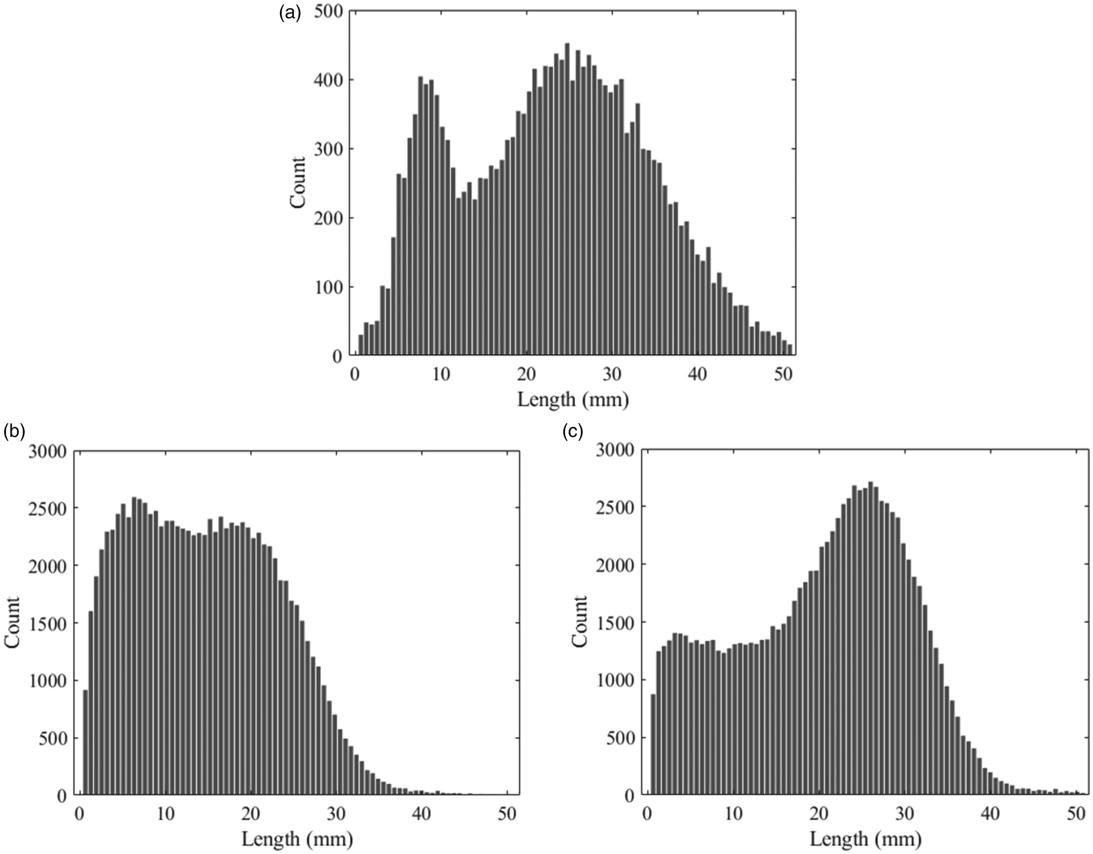
Histograms of fiber lengths generated from synthetic distributions that are used to test the algorithm: (a) Gaussian mixture; (b) Weibull mixture representing an immature/weak cotton and (c) Weibull mixture representing a mature/strong cotton.

Given the distributions (i.e. ground truth), we can compute the complete fibrogram using the sampled data. As such, we first tested the reconstruction method without estimating the beginning of the curve, which is typically missing from HVI fibrograms. This shows how effectively the algorithm can recover the original distribution in an ideal scenario. In this case, all that is needed is the windowed, curve-fitting procedure for which we use a cubic polynomial equation (9) and a window size $w =$ 6.985 mm. Then, the fibrogram data is removed between 0 and 3.81 mm, simulating what is output by an USTER HVI 1000. The algorithm is then re-applied using the following parameters.
Cutoff $x_{c}$ = 6.35 mm (i.e. reconstruct the fibrogram from 0 to 6.35 mm).

The initial part of the curve is reconstructed using the exponential
$g (x) = a e^{b x + c}$
(12)

Equation (12) is estimated using fibrogram data from 6.35 to 12.7 mm.

Window size $w =$ 6.985 mm.

Curve-fitting procedure with a cubic polynomial equation (9).

Statistics calculated from the reconstructed distributions are compared to those calculated from the original histograms.

We should note that these algorithm parameters were chosen based on a combination of examining real fibrograms and experimentation with the simulated distributions. For example, the cutoff of 6.35 mm is based on the observed concavities at the beginning of the fibrogram discussed previously. The exponential, $g (x)$ , and the area of the fibrogram used to estimate it experimentally provided a close approximation to the first part of the fibrogram for simulated data. The window size and choice of curve to fit work together to some extent. We chose a third-order polynomial to hopefully fit a more nuanced curve than a quadratic. A higher order curve (fourth, fifth, etc.) could potentially model the noise or concavities in the signal, which is exactly what we want to avoid. Also, since a third-order curve can be concave, the window size must be large enough such that the general trend of the curve within the window is convex—so that the resulting fit will also be convex. As we will show later, this combination of parameters produced good results; however, further research may necessitate some refinement in the future.

Visually examine reconstructed distributions

The purpose of this experiment is to visually examine the reconstructed distributions of different types of samples with well-known and distinct length properties. For that purpose, we selected five samples: two upland, two pima, and one viscose sample. The upland samples are commercial varieties—one grown in Oklahoma and the other from the Texas High Plains near Lubbock. The pima samples are also commercial varieties from California. The viscose sample—a man-made, cellulosic fiber sourced from Lenzing (Lenzing Fibers, Inc., Axis, AL, USA)—is specified as 38 mm in length with a linear density of 1.3 dtex. Each sample was tested on the HVI with a research protocol of 10 replications of length, including the fibrograms. All samples were conditioned for at least 48 hours at 21 ± 1°C and 65 ± 2% relative humidity (RH) prior to HVI testing. For each sample, we averaged the 10 fibrograms, then applied the reconstruction algorithm on the average fibrogram using the parameters specified for the simulated data above.

Comparison with HVI length parameters

For this experiment we were able to obtain 2497 commercial samples that were previously classed by the USDA-AMS. These samples represent varieties grown across the USA in 2021. Samples were tested on one HVI in the same manner as the previous experiment (a research protocol of 10 repetitions of length plus fibrograms) under the same environmental conditions. In this case, we applied the reconstruction algorithm on each individual fibrogram using the same algorithm parameters applied in the simulated data experiment. Statistics were calculated from the reconstructed distributions for each repetition and then averaged per sample. Similarly, the HVI measurements, ML, UHML, and UI, were averaged per sample. It should be noted that since the fibrogram is not a calibrated measurement, we compared all computed statistics from the fibrogram to the uncalibrated HVI measurements. (The HVI uses a two-point calibration method for length based on one long and one short reference cotton, resulting in linear correction equations for ML and UHML. The UI is not calibrated directly but is computed from the calibrated ML and UHML. Long and short standard cottons are established and provided by the USDA-AMS for use in HVI calibration.)

In addition, based on the fibrogram theory, the length distribution reconstructed from the fibrogram is by number. The AFIS produces both a length distribution by number as well as a length distribution by weight. This is accomplished by assuming constant fiber linear density. In general, this is an incorrect assumption; however, without additional information, this conversion is routinely used as an approximation. The following equation was used to convert the by-number length distributions to the by-weight approximation
$p_{w} (x) = \frac{x}{{M L}_{n}} p_{n} (x)$
(13)
where $p_{w}$ and $p_{n}$ are the distributions by weight and by number, respectively, ML_n is the ML by number (i.e. the mean of $p_{n}$ ), and $x$ is a given length.

Using both the by-weight and by-number distributions as well as the fibrogram span lengths suggested by Sayeed et al.,¹³ there are multiple ways of calculating the ML, UHML, and UI. Below is a list of statistics calculated for this experiment for each repetition and averaged per sample. The idea is to compare each one to the corresponding HVI measurement to establish a statistical interpretation of the HVI output.

Mean length:
ML_n—mean of the by-number distribution;

ML_w—mean of the by-weight distribution;

ML_SL—the 7.8% span length of the fibrogram.

Upper half mean length:
UHML_n—using the by-number distribution, mean length of fibers longer than the median;

UHML_w—using the by-weight distribution, mean length of fibers longer than the median;

UHML_a—(ASTM definition) mean length by number of the upper half by weight, that is, mean length by number of fibers longer than the median length from the by-weight distribution²²;

UHML_SL—the 1.8% span length derived from the fibrogram.

Uniformity index:
UI_nn—ratio of ML_n to UHML_n multiplied by 100 (by number);

UI_ww—ratio of ML_w to UHML_w multiplied by 100 (by weight);

UI_wa—ratio of ML_w to UHML_a multiplied by 100 (ML by weight and UHML by the ASTM definition);

UI_na—ratio of ML_n to UHML_a multiplied by 100 (ML by number and UHML by the ASTM definition);

UI_SL—ratio of ML_SL to UHML_SL multiplied by 100 (span lengths).

To be clear, the span lengths are taken from the fibrogram prior to the application of the algorithm. Recall from Figures 2 and 6 that the fibrogram produced by the HVI is normalized such that a value of 100% is assigned to the length at which scanning begins: 3.81 mm. Since the algorithm extrapolates the missing 3.81 mm, these extrapolated values are above 100%, thereby requiring re-normalization of the fibrogram. Rescaling the y-axis subsequently alters the location of the 7.8% and 1.8% span lengths.

Results

Simulated data

The fibrograms calculated from equation (2) and discretized for each of the three simulated distributions are shown in Figure 9. The differences between each of the fibrograms are reasonable based on the distributions shown previously in Figure 8. The bimodal Gaussian mixture clearly has the longest fibers and, as such, its fibrogram extends farther to the right than the other two. The distribution simulating a mature/strong sample has the next longest fibers, which is also apparent in the fibrograms. Finally, the distribution simulating an immature/weak sample has much more shorter fibers and, accordingly, its fibrogram is below the other two.

Figure 9.
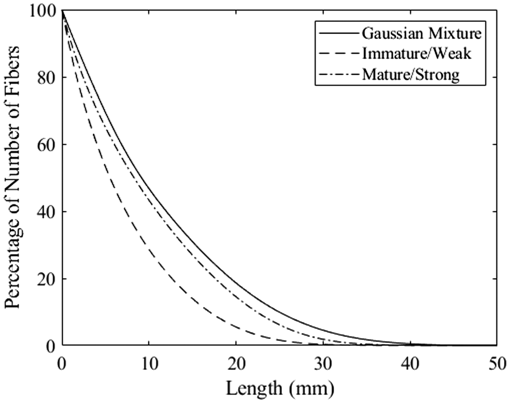
Fibrograms calculated from equation (2) for each of the three simulated distributions.

As mentioned, initially the algorithm was applied to each of these fibrograms without first reconstructing the beginning of the curve. Then the fibrogram was truncated at 3.81 mm and re-normalized to simulate the fibrograms produced by the HVI. With the truncated fibrogram, the initial part of the curve was reconstructed using equation (12), as described in the Experimental methods section. Figure 10 shows the results of the reconstructed distributions for each fibrogram before and after truncating the fibrogram. Also, the resulting distributions are superimposed over the histogram of the original data. 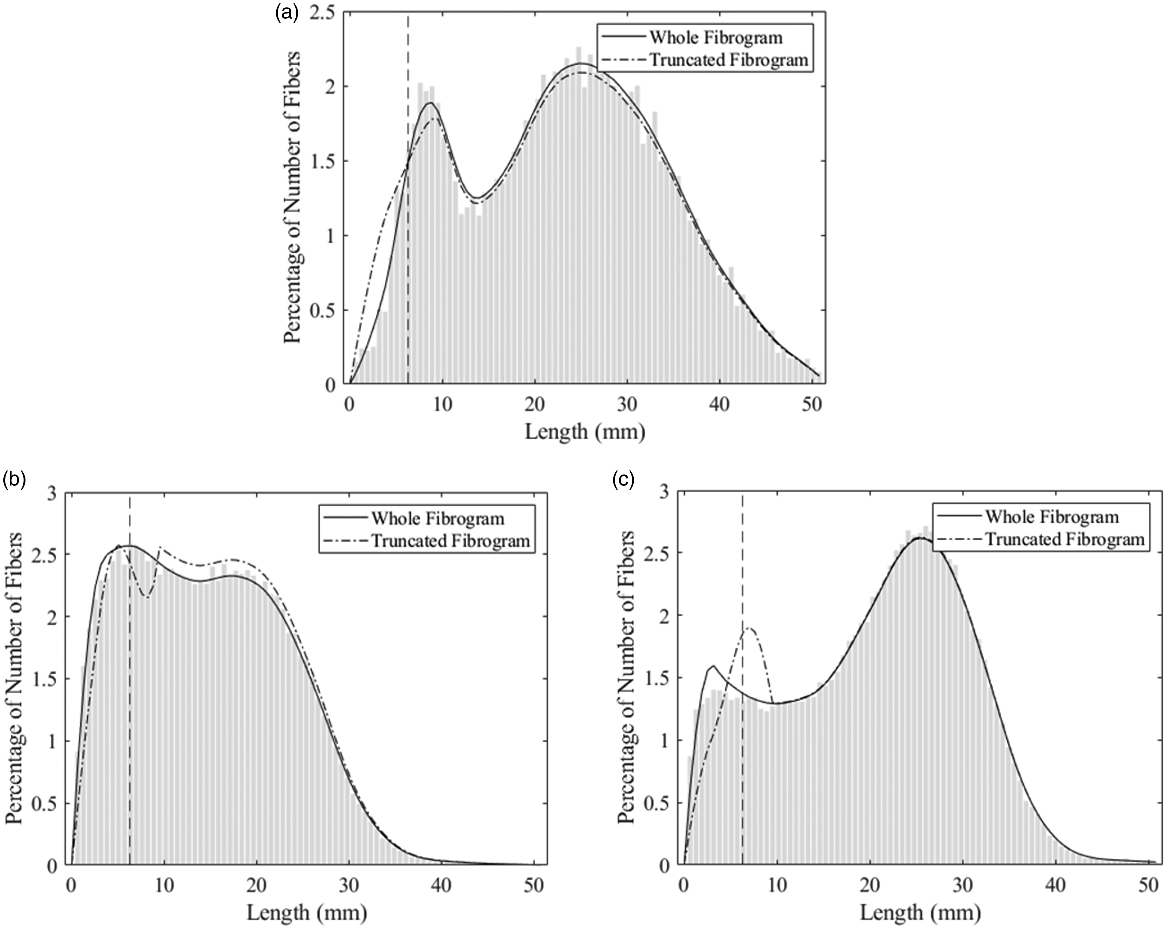The vertical, dashed line at 6.35 mm indicates the cutoff, $x_{c}$ , that is, the data to the left was estimated using equation (12) for the truncated fibrogram. In all three cases, the reconstructed distribution from the whole fibrogram (solid black line) follows the histogram quite closely.

Figure 10.
Reconstructed distributions from fibrograms (before and after truncating) for each type of distribution superimposed over the original histogram. The cutoff at 6.35 mm is shown by a dashed, vertical line: (a) Gaussian mixture; (b) Weibull mixture representing an immature/weak cotton and (c) Weibull mixture representing a mature/strong cotton.

The reconstructions based on the truncated fibrograms (dash-dotted line) are also close; however, as expected, there are some deviations before or near the cutoff. For the Gaussian mixture distribution in Figure 10(a), visually, the differences between the two reconstructions are relatively small. This is likely because the distribution is Gaussian, an exponential function, and can be modeled quite well with equation (12). The other two examples, the immature/weak and mature/strong distributions (Figures 10(b) and (c), respectively), exhibit greater deviations—particularly around the cutoff at 6.35 mm. This is due to the lack of smoothness at the point where the estimated curve using equation (12) joins the original fibrogram curve. This issue becomes amplified due to the two orders of differentiation between the fibrogram and the distribution. Nevertheless, the rest of the reconstructed distribution to the right of the cutoff follows the original very closely for both Weibull mixtures.

As part of the algorithm, the CDF, $Y (x)$ , is also calculated simultaneously with the distribution. This function is useful for calculating percentiles such as the median, that is, the 50th percentile. Figure 11 shows the differences between the three curves generated from the original distribution, the whole fibrogram, and the truncated fibrogram for each distribution type. In each case, the difference between the CDF calculated from the original distribution and the CDF output by the algorithm based on the whole fibrogram is visually indiscernible. However, there is a slight difference for the CDF based on the truncated fibrogram in each case. For the Weibull mixture representing the mature/strong cotton in Figure 11(c), the difference is only noticeable from 0 to ∼8 mm.

Figure 11.
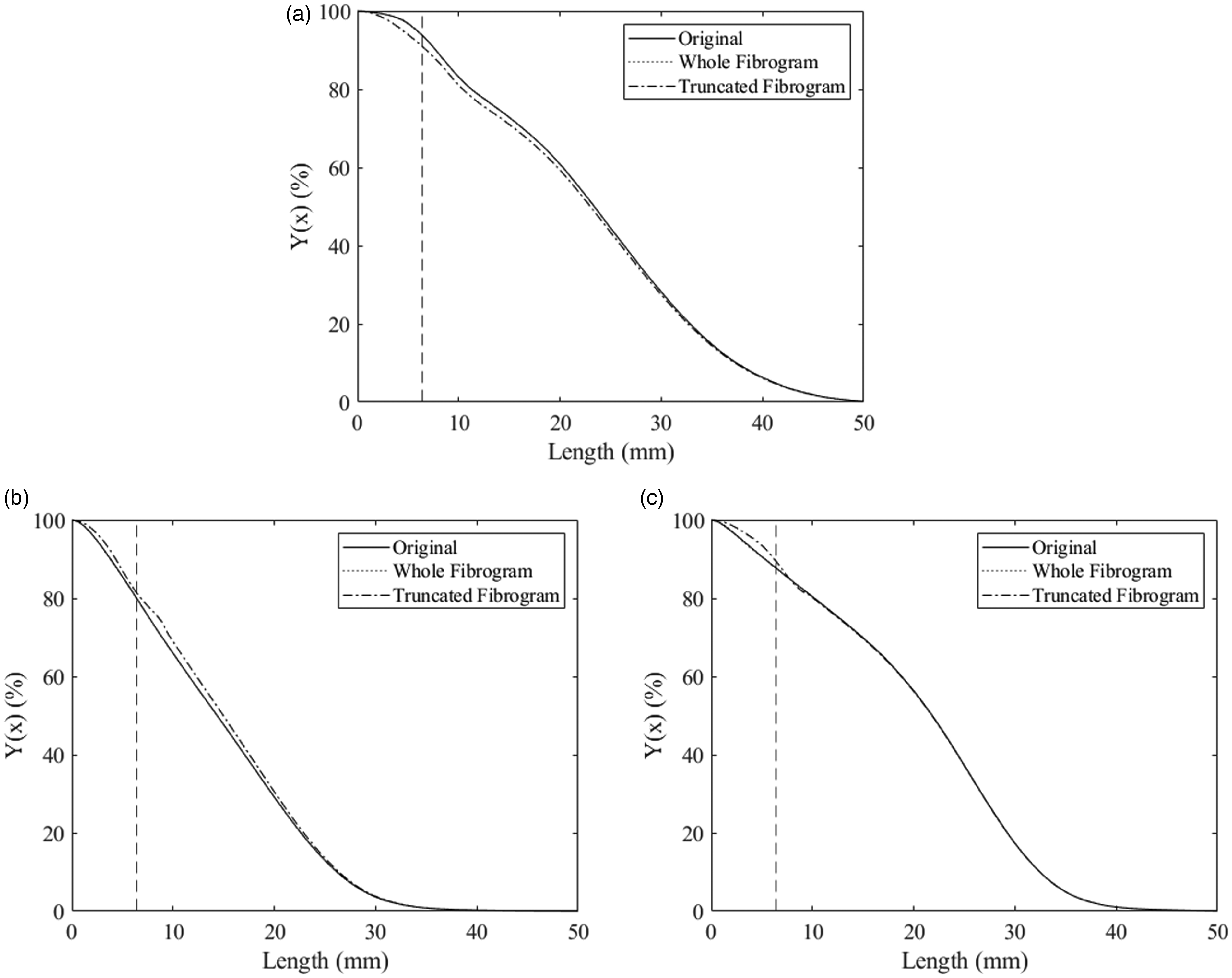
Cumulative distribution function (CDF), $Y (x)$ , for each of the distribution types. Each graph shows the CDF computed from the original distribution (solid black line), the CDF output by the algorithm using the whole fibrogram (dotted line), and the CDF based the truncated fibrogram (dash-dotted line). The location of the cutoff at 6.35 mm is shown by a vertical, dashed line: (a) Gaussian mixture; (b) immature/weak and (c) mature/strong.

It is necessary to point out that we have not shown the reconstructed fibrograms resulting from the application of the algorithm because the differences between the original fibrogram and reconstructed fibrograms based on the whole or the truncated original fibrogram are visually indiscernible. The fibrogram and the distribution are two orders of differentiation apart. Note how close the curves are for the CDFs (Figure 11), while the differences in the PDFs are quite obvious (Figure 10). Going from the CDF to the fibrogram is another level of differentiation meaning the curves will get even closer, making them appear to be practically the same unless zoomed in to small portions of the fibrograms. Here, we are focusing on the differences in the PDFs because that is where we see the errors amplified in the reconstruction and where most of the statistical properties are derived.

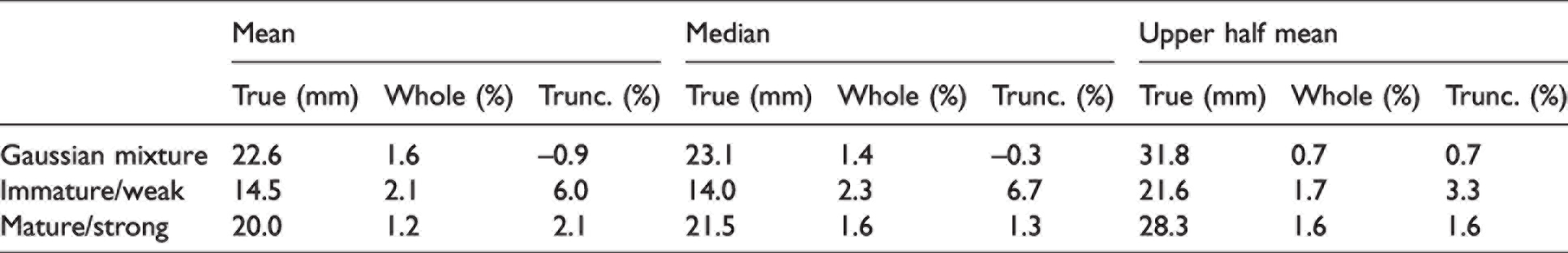
In addition to visually evaluating the results of the method, statistics were calculated from the reconstructed distributions as well as the CDF and compared to the statistics of the original synthetic data. While access to the distribution and CDF grants the ability to calculate a wide variety of statistical parameters, for the scope of this discussion we are limiting those to the ones used in calculating parameters that are related to HVI length output: mean, median, and upper half mean (i.e. mean of values greater than the median). Furthermore, while a later experiment approximates a distribution by weight, here we focus solely on the direct output of the algorithm, which is a distribution by number. Table 1 shows results of these three statistics calculated from the reconstructed distributions based on the whole fibrogram and the truncated fibrogram compared to the true value calculated from the original synthetic data. The comparisons are expressed as a percentage of the true value. When using the whole fibrogram curve as a basis for the reconstruction, statistics computed from the recovered distribution differ by no more than 2.3% of the true value. This error is likely attributed to the smoothing effect of the reconstruction process, which is visible in the results in Figure 10 and is practically negligible. Results are similar with the truncated fibrogram except for the immature/weak Weibull mixture, which differs by as much as 6.0% and 6.7% from the true value for the mean and median, respectively. This is likely due to a larger percentage of the original distribution existing to the left of the cutoff, which has to be estimated. Perhaps the estimation of the region from 0 to ∼7 mm is less accurate for samples with a high percentage of shorter fibers; however, it should be noted that this example of an immature/weak cotton represents an edge case with maturity ratio = 0.76 and strength = 22.3 g/tex.²¹ (In the 2021 US crop, only 30 bales out of 16.6M bales show a reported strength of 22.3 g/tex or less according to EFS® USCROP™ data.²³) On the other hand, the other two distribution types, which have far fewer shorter fibers, produced more accurate results after truncating the fibrogram.

Table 1.
Mean, median, and upper half mean calculated from the reconstructed distributions based on the whole fibrogram (Whole) and the truncated fibrogram (Trunc.) compared to the true value calculated from the original distribution (True); comparisons are expressed as a percentage of the true value

Mean
Median
Upper half mean

True (mm) Whole (%) Trunc. (%) True (mm) Whole (%) Trunc. (%) True (mm) Whole (%) Trunc. (%)

Gaussian mixture 22.6 1.6 –0.9 23.1 1.4 –0.3 31.8 0.7 0.7

Immature/weak 14.5 2.1 6.0 14.0 2.3 6.7 21.6 1.7 3.3

Mature/strong 20.0 1.2 2.1 21.5 1.6 1.3 28.3 1.6 1.6

Visually examine reconstructed distributions

The three types of samples selected for this experiment were chosen due to their known and well-understood differences in length distribution. The reconstructed distributions for these samples are shown in Figure 12. Also, the average HVI length parameters for these samples are shown in Table 2. Visually, there is a clear difference between the reconstructed distributions for each of these types of samples. The pima samples (Figure 12(b)) show a greater number of longer fibers and fewer shorter fibers than the upland samples (Figure 12(a)). This makes sense, as pima is known as an “extra long staple” cotton. Also, pima is stronger than upland and subject to less aggressive mechanical ginning (roller gin versus saw gin for upland), resulting in fewer short, broken fibers. The viscose distribution (Figure 12(c)) is interesting since, theoretically, as a man-made, monolength fiber, the distribution should be an impulse function at 38 mm (the specified length). However, prior to testing, the sample was subjected to a mechanical opening and carding process, which breaks some fibers. Nevertheless, the reconstructed distribution of the viscose sample is in stark contrast to the four cotton samples. The very narrow mode around 35 mm plus a very low number of shorter (broken) fibers makes sense for this type of sample.

Figure 12.
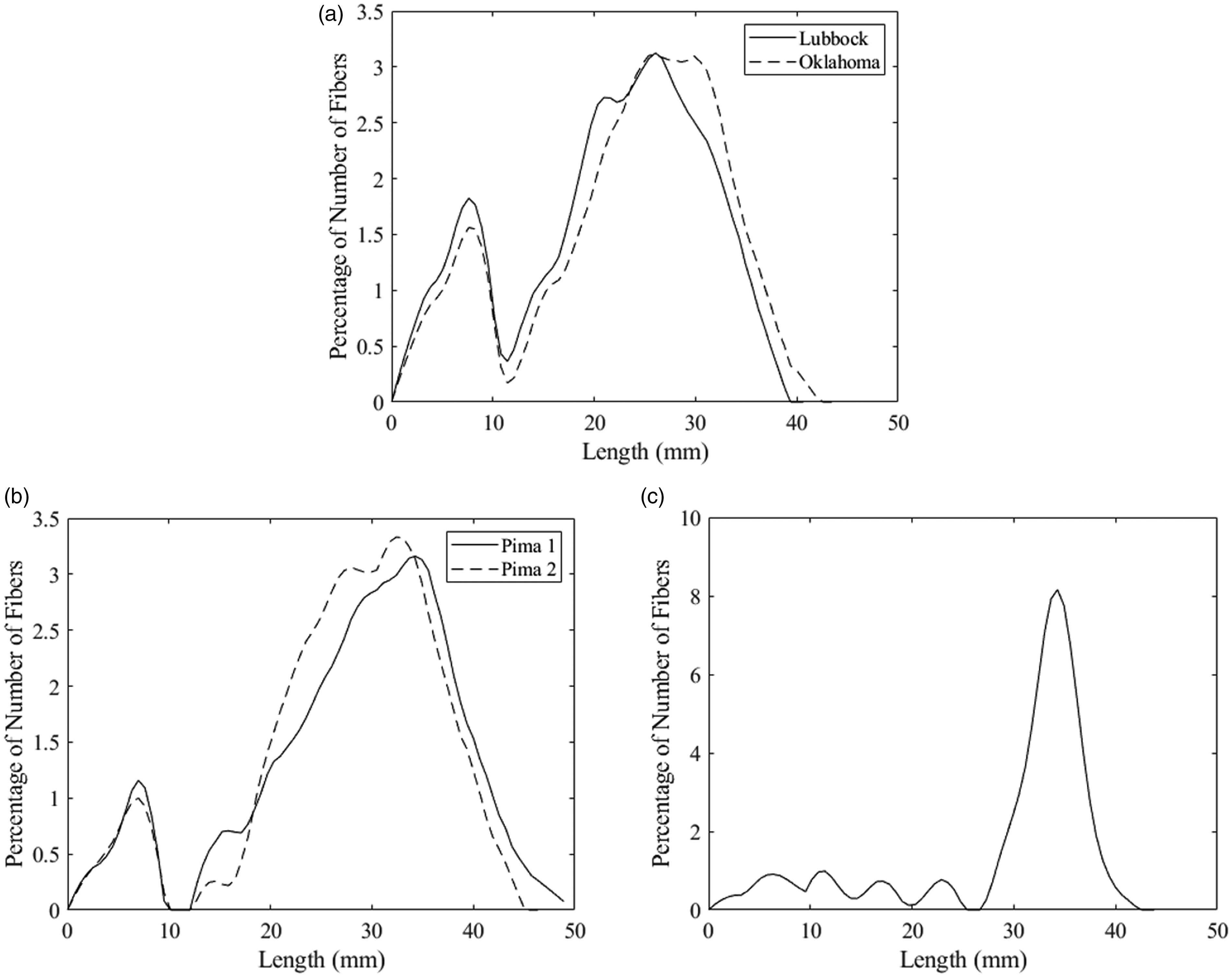
Visual examples of reconstructed distributions from three types of samples: (a) upland cotton; (b) pima cotton and (c) viscose.

Table 2.
Average High Volume Instrument length parameters for the five samples shown in Figure 12

UHML (mm) UI (%)

Upland (Lubbock) 30.8 81.5

Upland (Oklahoma) 31.7 83.0

Pima 1 36.4 85.1

Pima 2 35.1 84.7

Viscose 34.3 91.4

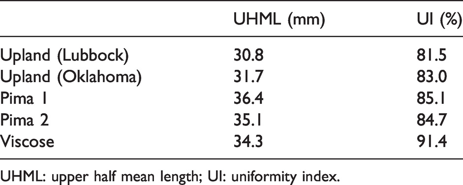
UHML: upper half mean length; UI: uniformity index.

Comparison with HVI length parameters

For the 2498 commercial samples, the results for comparing different methods of calculating the ML to the uncalibrated HVI ML are shown in Figure 13. In each of these graphs, a dashed line shows equality (y = x), and the solid black line indicates the regression line corresponding to the displayed equation and coefficient of determination (R²). Clearly, as has been previously reported, it seems that the HVI ML is derived directly from the 7.8% span length of the fibrogram (Figure 13(c)), as all data practically lies along the equality line with R² = 0.999. However, it appears that ML_w (Figure 13(b)) is more similar to the HVI ML than ML_n (Figure 13(a)), based on the reconstructed distribution. Nevertheless, in either case, these graphs indicate that the parameters calculated from the reconstructed distribution are highly correlated with the current HVI output with R² values of 0.868 and 0.960 for ML_n and ML_w, respectively.

Figure 13.
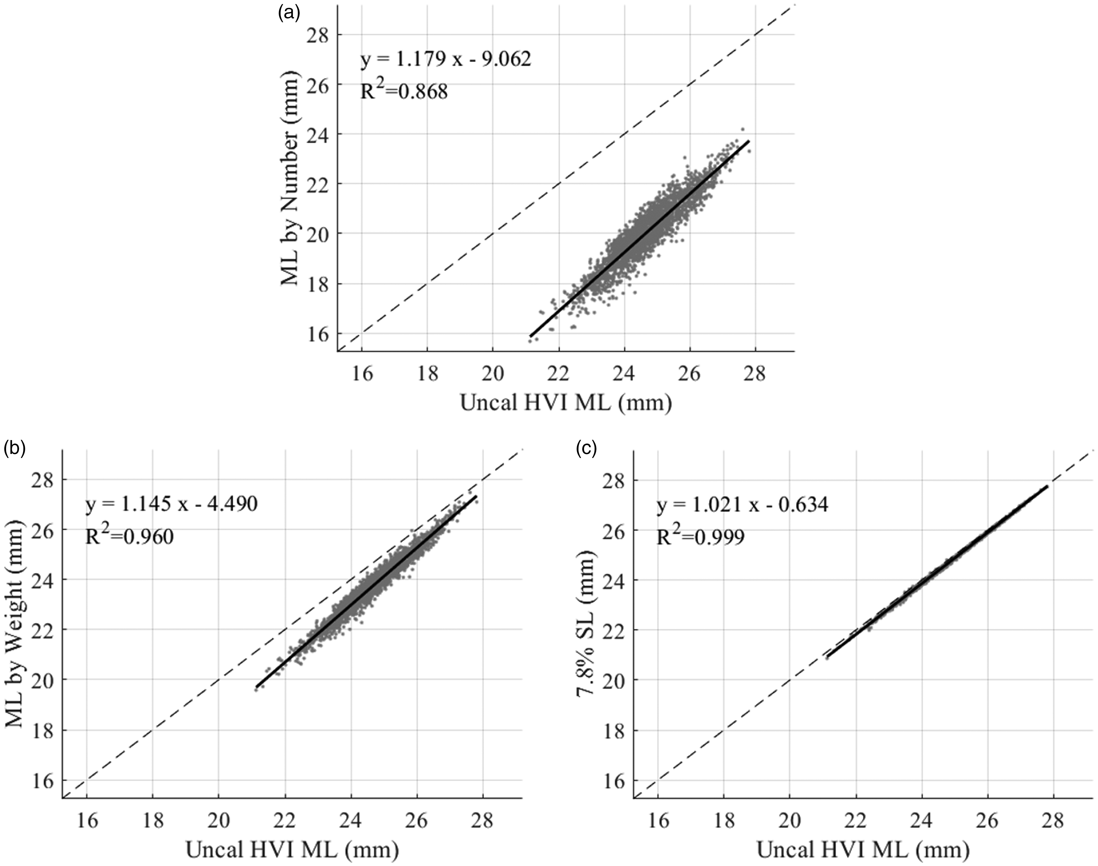
Comparison of different methods of calculating the mean length (ML) to the uncalibrated High Volume Instrument (HVI) ML for 2498 commercial samples. The dashed line represents equality. The solid black line shows the regression line for the displayed equation and associated coefficient of determination: (a) ML by number; (b) ML by weight and (c) 7.8% span length.

The results for comparing methods for calculating the UHML are shown in Figure 14. Here, again, all three statistics based on the reconstructed distribution (Figures 14(a)–(c)) show a very high correlation with the HVI output—R² ranges from 0.867 to 0.965. Among those three methods, both the UHML_w (Figure 13(b)) and UHML_a (Figure 13(c)) are very close to the uncalibrated HVI output, with very little difference between those two. Also, Figure 14(d) provides additional evidence that the HVI derives the reported UHML from the 1.8% span length of the fibrogram (R² = 0.998).

Figure 14.
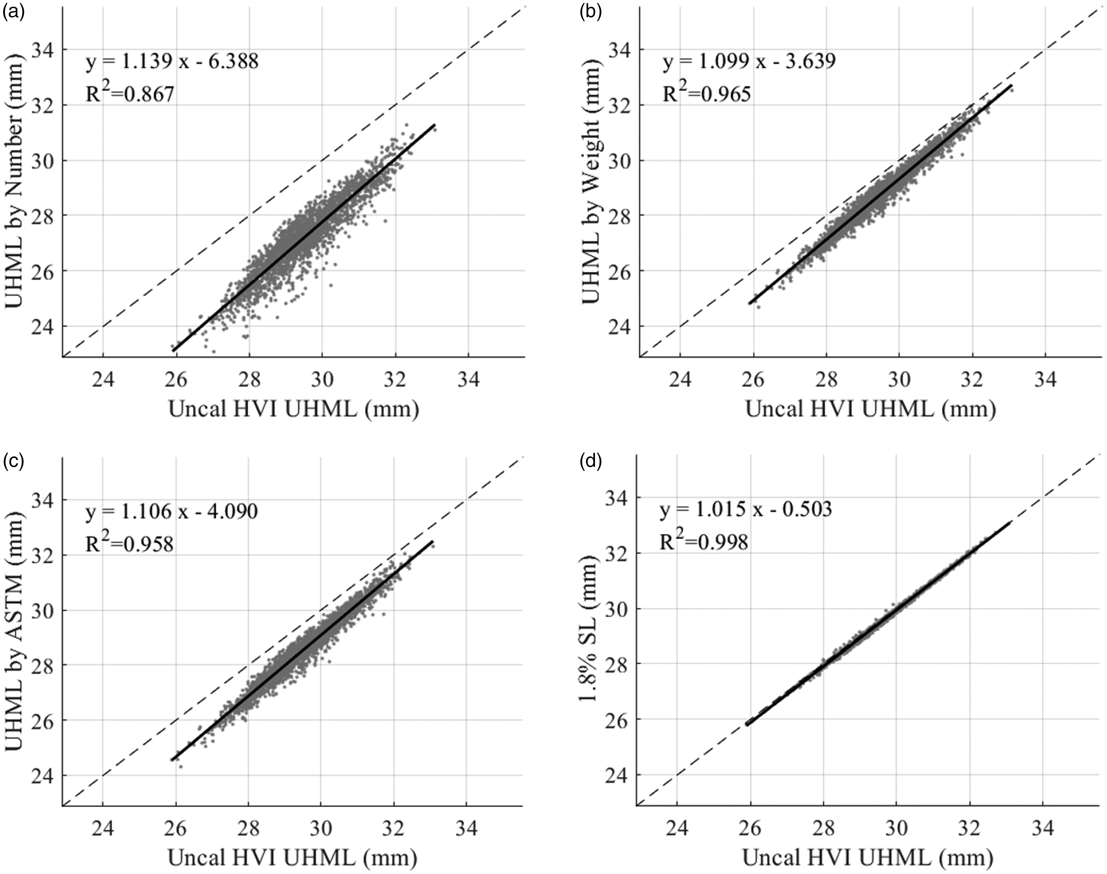
Comparison of different methods of calculating the upper half mean length (UHML) to the uncalibrated High Volume Instrument (HVI) UHML for 2498 commercial samples. The dashed line represents equality. The solid black line shows the regression line for the displayed equation and associated coefficient of determination: (a) UHML by number; (b) UHML by weight; (c) UHML by ASTM definition and (d) 1.8% span length.

Finally, the results for comparing methods for calculating the UI are shown in Figure 15. Note that in these results, “uncalibrated HVI UI” refers to the UI calculated from the uncalibrated ML and UHML, as the HVI does not directly calibrate the UI. All four methods based on statistics from the reconstructed distributions (Figures 15(a)–(d)) have a good correlation with the uncalibrated HVI UI, with R² ranging from 0.730 to 0.794. The two UI methods that are based mostly on the by-weight distribution, UI_ww (Figure 15(b)) and UI_wa (Figure 15(d)), are closer to the HVI output than UI_nn (Figure 15(a)) and UI_na (Figure 15(c)). Lastly, as the previous results show, the UI based on the span lengths (Figure 15(e)) is practically the same as the HVI output.

Figure 15.
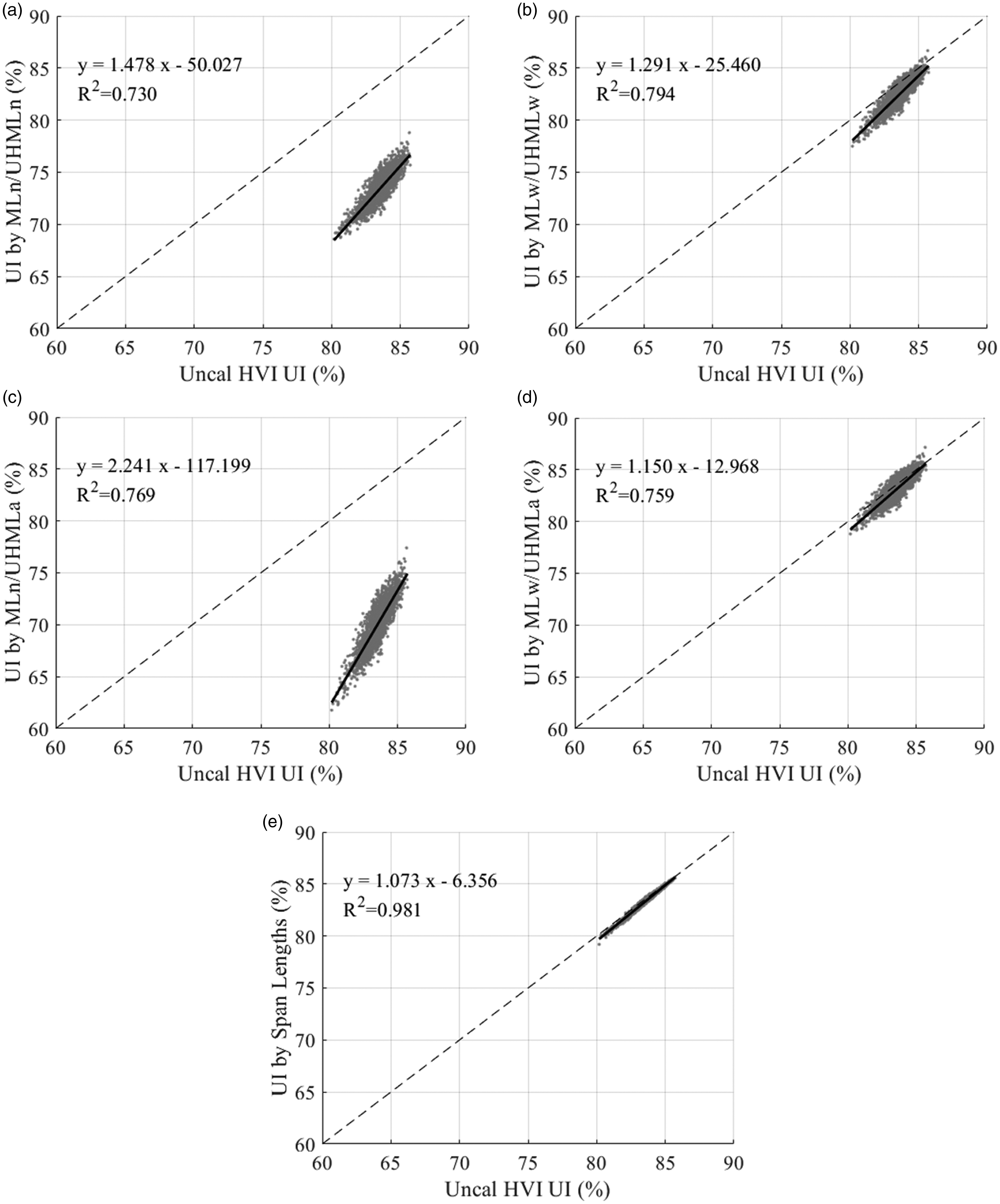
Comparison of different methods of calculating the uniformity index (UI) to the uncalibrated High Volume Instrument (HVI) UI for 2498 commercial samples. The dashed line represents equality. The solid black line shows the regression line for the displayed equation and associated coefficient of determination: (a) UI by number; (b) UI by weight; (c) UI calculated from mean length (ML) by number and upper half mean length (UHML) by ASTM; (d) UI calculated from ML by weight and UHML by ASTM and (e) UI by span lengths.

Conclusion

The current HVI length parameters only provide information regarding the longest fibers in the sample. Despite the names UHML and ML, little was known about how these HVI-measured values relate to the distribution of fibers in the sample. Moreover, it has been shown that additional fiber length information is present in the fibrogram produced by the HVI as it relates to yarn quality.¹³ As such, the ability to extract additional, meaningful information from the fibrogram would add value to the output currently provided by the HVI.

In this paper, we presented an algorithm based on established fibrogram theory that can reconstruct the fiber length distribution of a sample from an HVI fibrogram. Using the distribution as well as the associated CDF, one can calculate any number of meaningful, statistical parameters regarding a sample. Our experimental results show that the algorithm is accurate when tested with synthetic data from different types of distributions. This result should be emphasized, as it indicates that the algorithm successfully applies the theory. Furthermore, we showed that the reconstructed distributions of three different types of samples—upland, pima, and viscose—differed in ways that followed a priori knowledge of their length distributions.

In the last experiment, we compared several methods of calculating HVI-like length parameters based on the reconstructed distributions of 2498 commercial samples. The results show that the current HVI measurements of ML and UHML are likely derived directly from the 7.8% and 1.8% span lengths, respectively, as has been reported by others.¹³ However, based on the theory presented above, fibrogram span lengths do not have a direct, interpretable relationship with the fiber length distribution. The proposed algorithm produces a length distribution by number, which can also be used to approximate a length distribution by weight, as is routinely carried out by the AFIS. While all the results of the various length parameters calculated from the reconstructed distributions show good correlations with the uncalibrated HVI output, the parameters based on an approximation of the distribution by weight are very close to the HVI measurements. Note that this does not imply that the HVI provides ML by weight or UHML by weight, per se, but this analysis offers a close statistical interpretation.

While these results are quite promising, there are several avenues of future research to pursue for further validation. For example, as previously mentioned, the AFIS currently produces a length distribution, which has become a de facto standard. (A method such as the Suter-Webb array would provide a true reference method; however, it is extremely time consuming and not conducive to testing large numbers of samples.²⁴) A comparison of AFIS distributions with distributions produced from fibrograms via the proposed method would be interesting. However, the experiment should be carefully devised, as the AFIS is known to break fibers due to its mechanical opening process, which changes the fiber length distribution. In comparison, the HVI fibrosampler is less aggressive in preparing the beard, thus potentially providing a more accurate measurement of the length distribution. Also, for further research, we plan to investigate yarn prediction models based on length parameters from the reconstructed distributions. Identifying parameters that relate to better yarn quality is the primary goal of this line of research. For example, shorter fibers are known to cause problems in spinning.³ Can we provide a measurement of short fibers based on the reconstructed distribution from a HVI that relates to yarn quality?

In summary, we believe this new method offers new possibilities for breeders and spinners. Future research will reveal whether length distributions reconstructed from fibrograms can offer the quality of information similar to the AFIS at the speed and reduced cost per test of the HVI.

	Mean	Median	Upper half mean
Gaussian mixture	22.6	1.6	–0.9	23.1	1.4	–0.3	31.8	0.7	0.7
Immature/weak	14.5	2.1	6.0	14.0	2.3	6.7	21.6	1.7	3.3
Mature/strong	20.0	1.2	2.1	21.5	1.6	1.3	28.3	1.6	1.6

	UHML (mm)	UI (%)
Upland (Lubbock)	30.8	81.5
Upland (Oklahoma)	31.7	83.0
Pima 1	36.4	85.1
Pima 2	35.1	84.7
Viscose	34.3	91.4

Footnotes

Declaration of conflicting interests

The author(s) declared no potential conflicts of interest with respect to the research, authorship, and/or publication of this article.

Funding

The author(s) disclosed receipt of the following financial support for the research, authorship, and/or publication of the article: This research was made possible through funding by the USDA-AMS (Project A20-187) and Cotton, Incorporated (Projects 17-531 and 17-533).

ORCID iDs

Christopher Turner

Md Abu Sayeed

References

El Mogahzy

Broughton

Lynch

WK.

A statistical approach for determining the technological value of cotton using HVI fiber properties. Text Res J 1990; 60: 495–500.

Elmogahzy

Chewing

CH.

Cotton fiber to yarn manufacturing technology: optimizing cotton production by utilizing the engineered fiber selection system. Cary, NC: Cotton Incorporated, 2001.

Thibodeaux

Senter

Knowlton

, et al. The impact of short fiber content on the quality of cotton ring spun yarn. J Cotton Sci 2008; 12: 368–377.

Cai

Cui

Rodgers

, et al. A comparative study of the effects of cotton fiber length parameters on modeling yarn properties. Text Res J 2013; 83: 961–970.

United States Department of Agriculture AMS. The classification of cotton. Agricultural Handbook 566 1999.

ASTM D5867-12:2020. Standard test methods for measurement of physical properties of raw cotton by cotton classification instruments.

Bechere

Zeng

Auld

Registration of five upland cotton mutant germplasm lines with superior fiber length, strength, and uniformity. J Plant Regist 2018; 12: 107–111.

Naoumkina

Thyssen

Fang

, et al. Genetic and transcriptomic dissection of the fiber length trait from a cotton (Gossypium hirsutum L.) MAGIC population. BMC Genom 2019; 20: 112.

Patel

Chandnani

Khanal

, et al. Pyramiding novel EMS-generated mutant alleles to improve fiber quality components of elite upland cotton germplasm. Ind Crops Prod 2022; 178: 114594.

10.

Bragg

Shofner

FM.

A rapid, direct measurement of short fiber content. Text Res J 1993; 63: 171–176.

11.

Kelly

Hequet

EF.

Variation in the advanced fiber information system cotton fiber length-by-number distribution captured by high volume instrument fiber length parameters. Text Res J 2017; 88: 754–765.

12.

ASTM D1447-07:2021. Standard test method for length and length uniformity of cotton fibers by photoelectric measurement.

13.

Sayeed

Schumann

Wanjura

, et al. Characterizing the total within-sample variation in cotton fiber length using the High Volume Instrument fibrogram. Text Res J 2021; 91: 175–187.

14.

Delhom

Kelly

Martin

Physical properties of cotton fiber and their measurement. In: Fang

(ed.) Cotton fiber: physics, chemistry and biology. Cham: Springer International Publishing, 2018, p.41–73.

15.

Sayeed

Kelly

Turner

, et al. Investigation of a multivariate correction method for HVI fibrogram measurements. Agron 2022; 12: 460.

16.

Tesema

Sayeed

Turner

, et al. An approach for obtaining stable, reproducible, and accurate fibrogram measurements from High Volume Instruments. Agron 2022; 12: 1120.

17.

Zhou

Wang

Wei

, et al. Extracting fiber length distributions from dual-beard fibrographs with the Levenberg–Marquardt algorithm. Text Res J 2020; 90: 37–48.

18.

Hertel

KL.

A method of fibre-length analysis using the fibrograph. Text Res J 1940; 10: 510–520.

19.

Chu

Y-T

Riley

CR.

New interpretation of the fibrogram. Text Res J 1997; 67: 897–901.

20.

Krowicki

Ramey

HH Jr.

An examination of the digital fibrograph length uniformity index. Crop Sci 1984; 24: 378–381.

21.

Krifa

Fiber length distribution in cotton processing: a finite mixture distribution model. Text Res J 2008; 78: 688–698.

22.

ASTM D123:2019. Standard terminology relating to textiles.

23.

EFS®-USCROP™. Version V8.7.000. Cotton, Inc., https://www.cottoninc.com/cotton-production/quality/efs-system-software/uscrop-software/ (2020, accessed November 2, 2020).

24.

ASTM D1440-07:2019. Standard test methods for length and length distribution of cotton fibers (array method).

	Mean			Median			Upper half mean
	True (mm)	Whole (%)	Trunc. (%)	True (mm)	Whole (%)	Trunc. (%)	True (mm)	Whole (%)	Trunc. (%)
Gaussian mixture	22.6	1.6	–0.9	23.1	1.4	–0.3	31.8	0.7	0.7
Immature/weak	14.5	2.1	6.0	14.0	2.3	6.7	21.6	1.7	3.3
Mature/strong	20.0	1.2	2.1	21.5	1.6	1.3	28.3	1.6	1.6

Reconstruction of the cotton fiber length distribution from a High Volume Instrument® fibrogram

Abstract

Keywords

A review of fibrogram theory

Algorithm description

Theory versus real world application

Algorithm details

Determining the end of the fibrogram

Estimating the beginning of the fibrogram

Curve fitting and reconstruction of the distribution

Experimental methods

Simulated data

Visually examine reconstructed distributions

Comparison with HVI length parameters

Results

Simulated data

Visually examine reconstructed distributions

Comparison with HVI length parameters

Conclusion

Footnotes

Declaration of conflicting interests

Funding

ORCID iDs

References