
Abstract
Conducting city-wide tests of intelligent transport systems (ITS) is a costly endeavor that requires extensive funding and planning. Combined traffic simulations can be utilized to alleviate initial costs, and allow easy parameterization to deduce real-world requirements. In this paper, we aim to contribute to two frontiers in the domain of traffic state estimation (TSE) within an urban environment. First, we introduce speed estimation and different sensor technologies, reiterating the foundations of traffic dynamics. Second, we present a simulation-based assessment utilizing the open-source co-simulation framework Eclipse MOSAIC, alongside a newly developed TSE application suite, executed on top of the BeST Berlin traffic scenario. This evaluation highlights the estimation capabilities of different sensor technologies and speed estimates in an urban scenario, addressing their effectiveness in various city areas.
1. Introduction
Traffic simulation has long been an important tool for investigating potential road and junction layouts, new traffic signal control strategies, and novel traffic efficiency solutions. However, many ideas in this domain rely on additional factors such as vehicle-to-everything (V2X) communication and sensor models. Co-simulation is suitable for mixing and matching simulators according to requirements at hand. Numerous state-of-the-art simulators exist in the open-source world covering each domain. Eclipse SUMO 1 is a prominent open-source traffic simulator, while ns-32 and the INET framework for OMNeT++ 3 are popular in the communication domain (LTE/5G and ITS-G5). Over the past decade, we actively developed and improved the co-simulation environment Eclipse MOSAIC. 4 A special effort was put into coupling important simulators to provide a coherent evaluation tool for the research of novel intelligent transport systems (ITS).
Traffic state estimation (TSE) is an excellent research topic suited for simulation, as the sensor infrastructure can be costly to install, and much data have to be gathered before yielding results. In this paper, we present a simulated evaluation setup suited for complex analysis of TSE in urban environments.
First, we give a theoretical introduction into the field of traffic dynamics, focusing on the commonly applied sensor technologies for induction loops and floating card data (FCD), and implied estimation methods. Induction loops measure speeds at fixed positions, while FCD relies on user participation. Judging the effectiveness of these sensor modalities boils down to a comparison of the installation costs of fixed infrastructure against the required amount of user participation. User participation in the context of ITS is commonly referred to as market penetration rate, and finding minimal requirements often is a central research question.
Second, we put the theoretically discussed fundamentals into practical use. For this purpose, an application and evaluation toolkit, published in previous research,5,6 are utilized. The significance of any simulation study is highly dependent on the validation of its underlying models. In our use case, this requires a strong trust in the traffic models, road networks, and simulated traffic volumes. Therefore, we execute our evaluation in the open-source BeST scenario, a calibrated representation of 24 h of motorized traffic in Berlin, Germany. 7 The scenario is built for SUMO, which, has been shown to deliver accurate representations of real-world traffic patterns. 8 Combined, we leverage an extended MOSAIC in conjunction with the BeST scenario to conduct a study in the area of Berlin-Charlottenburg.
In addition to the initial study of distinctive areas, we aimed at a global investigation. Therefore, we examine travel times as a proxy measure for global TSE quality.
This paper is an extended version of Schweppenhäuser et al. 5 and is structured as follows. First, we describe the theoretical basis. Initially, section 2 gives a broader introduction to relevant topics of traffic dynamics. Next, we explain the applied sensor modalities and their implications for estimation methods in section 3. Second, practical considerations are explained. In section 4, we present the TSE toolkit and explain the simulation setup. Conducted experiments and results are described in section 5. Finally, in section 6, we summarize our findings and highlight our future research interests.
2. Fundamentals of traffic dynamics
This section builds on common traffic theory terminology. Newer readers are encouraged to refer to the following references for difficulties.9,10,11
Traffic dynamic research often uses so-called space–time diagrams to explain spatiotemporal relations of the traffic flow. 10 Figure 1 depicts two such space–time diagrams. Conventionally, we plot the time on the abscissa and the space on the ordinate. Each of the purple lines represents the trajectory of a vehicle moving along a given route, where steeper segments indicate faster speeds and less steep segments indicate lower speeds. From a given trajectory, it is trivial to calculate the average velocity for a segment of its route using Equation (1) as follows:
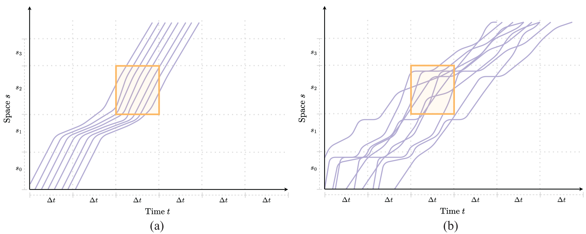
Exemplary space–time diagrams. 5 (a) Space–time diagram highway. (b) Space–time diagram urban road.
As the traffic state is a highly fluctuating measure, deviating both over space (i.e., different roads/road segments) and over time (i.e., morning and evening peaks versus midday lows), any statement about it has to be made on segments in space and time. Empirically speaking, this means that we consider separate time intervals and traffic network segments, leading to spatiotemporal measurements. This also implies that over these intervals and segments, some form of aggregation has to be applied. Usually, one sets a constant aggregation interval (
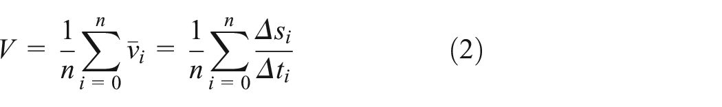
where
Figure 1(a) and (b) illustrates that estimating traffic state on highways is simpler than on urban roads. 12 On highways, driver behavior is fairly consistent. In contrast, urban roads have large variances in speed, acceleration, and braking due to factors like traffic signals, second-row parking, and other obstructions, increasing complexity.
3. Sensor modalities
In this section, we will describe the basic functionality and implied use cases of the sensor modalities under test, starting with induction loops and later moving on to FCD. We explicitly regard these sensor modalities separately and omit considerations of fusing the acquired sensor data, as we aim to make out the strengths and weaknesses independently. The interested reader may find approaches for fusing sensor data in TSE applications in the literature.13,14
3.1. Induction loops
The most widespread, traditional sensor modality comes in the form of induction loops, also known as spot or loop detectors. They function by insetting two metal coils within a short distance from each other below the surface of a road. Using the principle of induction, it is possible to detect when a vehicle passes a coil. By knowing the distance between the two coils and stopping the time at passing, one can determine the spot speed of a vehicle with high precision.
Due to the high installation price, loop detectors are very sparsely installed and mostly cover major road arteries. In addition, road administrators usually abstain from installing more than one detector per road segment, which limits insights into the roads’ traffic.
Knowing about the operation and costs of induction loops, we can revisit the space–time diagram from the fundamentals in section 2 and illustrate how one would aggregate the mean speed using a loop detector. Figure 2(a) depicts this by drawing a cross-section through the middle of
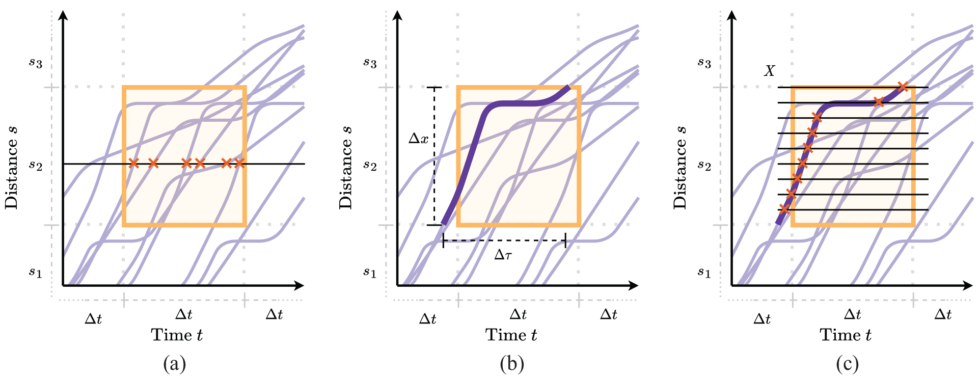
(a) Loop mean speed. (b) Temporal mean speed. (c) Spatial mean speed. 5
Intuitively, to aggregate the marked spot speeds within the marked
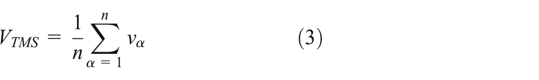
where
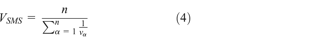
Note, that even though both presented speeds, especially the space mean speed, are intensively used in practical traffic density analysis, they rarely deliver correct results for density. In reality, density estimates using the time mean speed tend to underestimate the actual density, whereas estimates using the space mean speed tend to overestimate the actual values. For in-depth explanations on these circumstances see the work of Treiber and Kesting 10 (Chapter 5).
Another important aspect of the time and space mean speed is that they originate from traffic-flow theory, which treats moving vehicles similar to a hydrodynamic process in which flow, density, and speed of particles (i.e., vehicles) have a strong correlation. Treating vehicles as particles works sufficiently well on highways, where there is little variance in vehicle speeds and a certain degree of predictability in vehicle movements. In urban scenarios, however, using a single point of measurement will often fail at giving a meaningful insight into the realizable mean speed. The inhomogeneous trajectories in Figure 2(a) further illustrate this potential flaw.
3.2. FCD
With the increasing availability of GNSS-enabled (Global Navigation Satellite System) devices and broader cell coverage, people began to use vehicles as moving (i.e., floating) sensors in the early 2000s. 15 By periodically transmitting position, speed, and heading data to a central service via the cellular network, many vehicles provide a data set called FCD. This method of data collection became the de facto standard for many traffic services and is applied in current-day navigation applications such as Google Maps and TomTom.
Nonetheless, utilizing the data received from connected vehicles comes with a set of difficulties. On one hand, sensor inaccuracies, especially those of GNSS sensors, impose a large threat on the validity of collected data. Instead of just trying to improve sensor technologies (e.g. by fusion of GNSS and Inertial measurement systems), an approach called map-matching 16 is applied, where the vehicle trajectories are combined with a digital map to infer their most probable positions regarding coordinates but also respective edge and lane positions. The second major difficulty is the market penetration rate, which refers to the percentage of vehicles equipped with the necessary technology to provide FCD. A higher market penetration rate implies more data points and, consequently, more accurate TSE. For example, commonly cited thresholds for reliable highway estimation range from 5% to 10% market penetration, 12 meaning that every 20th vehicle needs to be connected. In an urban city scenario, this value increases due to higher fluctuations and less coverage in residential areas.
When using FCD as the data source, multiple approaches for mean speed estimation can be applied. These approaches typically examine and aggregate each road segment (i.e., edge or sub-edge) individually by recognizing traversals of the said segments.
Commonly, some form of curve fitting is applied using either interpolation or regression (i.e., using polynomial splines) to estimate vehicle movements between received FCD samples. A lower frequency of samples imposes higher uncertainty on the fitted curves. These fitted curves can then be used to infer speed values along a given edge for given vehicles. Yoon et al.
17
introduce the Temporal Mean Speed ((
The temporal mean speed is simply defined as “[...] the average speed over time [...].” 17 It captures the average speed for a single vehicle for one edge, which is visualized in Figure 2(b) and formalized in Equation (5) as follows:

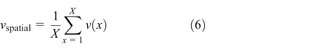
Yoon et al.
17
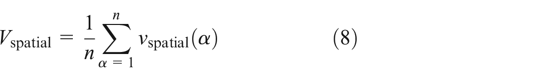
define the spatial mean speed as “[...] the average speed over location [...].” However, compared with the temporal mean speed, the spatial mean speed follows a more difficult definition as shown in Equation (6). In this equation,
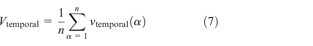
As mentioned previously, one is usually interested in an aggregated view of the traffic state as compared with those of individual vehicles. Aggregating the temporal and spatial mean speed for a given time segment has the caveat that traversals of the inspected edge may start before a given time segment. This issue is also visualized in Figure 2(b), where the highlighted vehicle trajectory driving on segment
Alternative approaches may omit the curve-fitting step and directly average and aggregate collected samples. These approaches do not face the aforementioned issue, though they can tend to oversimplify the TSE task as only temporal features will be regarded.
4. Simulation approach
To evaluate, compare, and parameterize a TSE model, simulation-based tests can be an effective tool before considering a real-world deployment. Simulation not only allows to catch potential errors and privacy threats at a much lower cost, but it also allows an evaluation of the necessary market penetration rates for a functioning system.
4.1. TSE applications for Eclipse MOSAIC
For simulative tests to deliver significant results, simulators for traffic, communication, and other environmental influences have to be modeled as close to reality as possible. The MOSAIC simulation framework18,4 couples industry-leading FOSS (Free and Open-Source Software) simulators from these domains using a runtime infrastructure based on the IEEE standard for high-level architecture (HLA). MOSAIC, additionally, provides a powerful application simulator that allows for fast prototyping and integration of applications in the domains of smart mobility including V2X Communication via ITS-G5 and LTE/5G, autonomous vehicle perception, and e-mobility.
For our evaluation purposes, we couple the microscopic traffic simulator Eclipse SUMO 1 with MOSAIC’s integrated Application and Cell simulators. Based on the general FCD approach, we modeled the system using MOSAIC’s Application simulator (see Figure 3). The model includes a vehicle application that periodically sends FCD Updates consisting of individual FCD Records and a server application that receives, processes, and aggregates the said traces. The simulation-based approach allows for easy consideration of different market penetration rates of FCD, referring to the proportion of vehicles in the simulation that are equipped to send FCD updates.
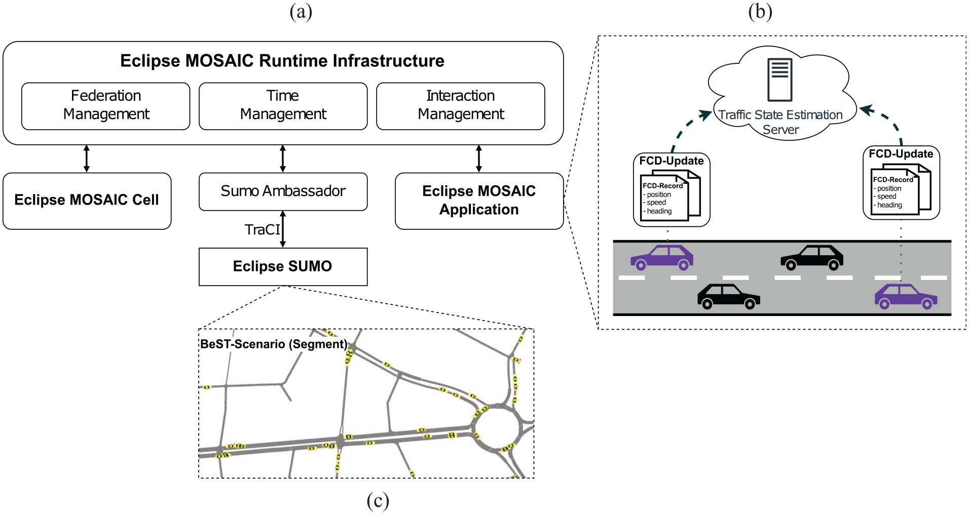
This diagram gives an overview of all relevant simulators and how they are utilized in hand with the TSE applications. (a) Simplified version of the MOSAIC architecture based on the HLA. (b) How the vehicle applications interact with the Traffic State Estimation server using FCD. (c) Functionality of the traffic simulator SUMO. We map our applications on the vehicles controlled by SUMO, which provides realistic FCD traces. 5
The server has been designed to be extensible with many processing units that can act based on newly detected edge traversals or in an event-based manner. The default setup comes enabled with a processor for calculating the relative traffic status metric (RTSM) defined by Yoon et al., 17 which uses the spatial and temporal mean speed in a threshold-based approach to rate the traffic state. The results of this processor will be stored in a local SQLite database for postprocessing and investigation of the collected data. All relevant parameters for both the vehicles and the server and its processors can be configured using respective JSON configurations, to inspect different key aspects of the system.
In addition to the application-based speed measures (
4.2. Experiment setup
To validate the developed applications and mean speed measurements, a traffic scenario has to be established that mimics the real-world road network and traffic patterns accurately. Therefore, we utilize the BeST scenario 7 for MOSAIC. It encompasses 24 h of individual motorized traffic in Berlin, with around 2.25 million vehicle trips.
As we are not focusing on a city-wide evaluation, we set up our simulation within the Charlottenburg area of the BeST scenario and simulated an entire day of vehicle movements with 200,000 independent trips.
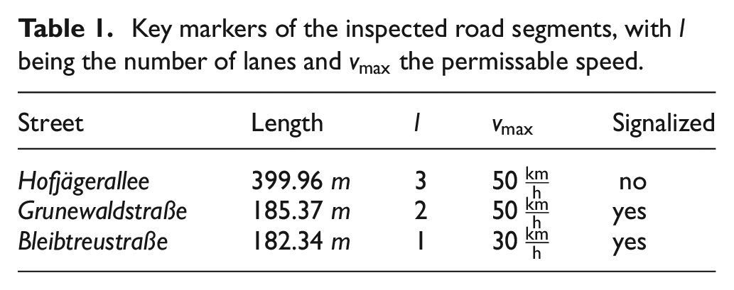
In this test, we configured 100% of vehicles with our FCD solution, set up loop detectors on the marked road segments in Figure 4, and collected estimations for the time and space mean speed using the configured SUMO output. We selected the marked roads intentionally, to obtain insights into how different measures react to different road types and sizes. Relevant markers for these roads are depicted in Table 1, which indicates how these roads differ from one another. Finally, we configured SUMO to write a file with reference speed values in the form of edge-wise data, which acts as our “ground truth.” This ground truth is calculated by recording all vehicle movements (including standing vehicles) within a given time interval and normalizing these values edge-wise for the said interval. While this ground truth provides a baseline for our simulations, it is highly dependent on the accuracy and reliability of SUMO’s vehicle models. We acknowledge the importance of validating these results against real-world conditions to ensure accuracy and reliability. All outputs were aggregated for 15-min intervals, as this window size offers a good trade-off between sufficient sample sizes and detailed enough granularity.
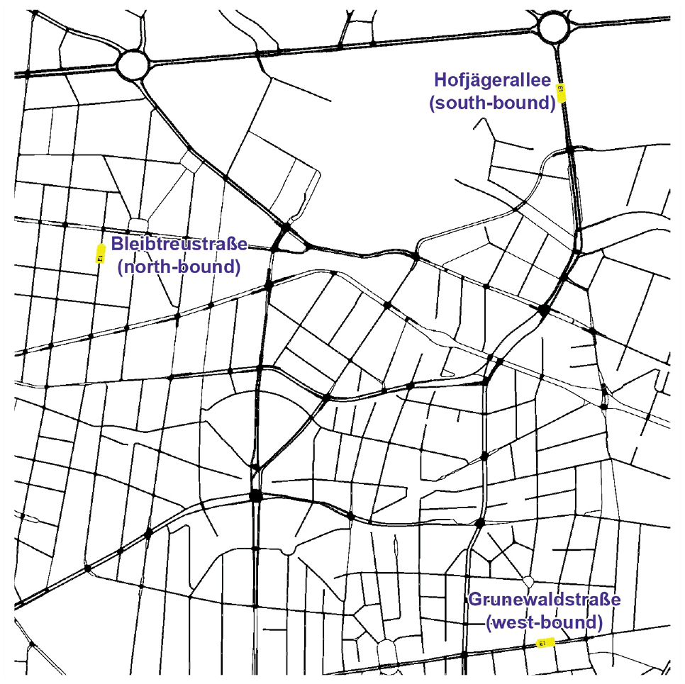
A map of Charlottenburg indicating loop detector positions for time and space mean speed estimations. 5
Key markers of the inspected road segments, with
4.3. Travel time estimation
After comparing TSE metrics for the selected road segments, we aimed at a broader evaluation. However, ranking the performance of a TSE metric globally, i.e., for the entire road network, is nontrivial due to the aforementioned variability in road characteristics and connected vehicle (CV) coverage. Intuitively, since we are concerned with mean speed estimates, an analysis of the resulting travel times is a valid approach. If more accurate travel time estimates are achieved, a globally better quality of the TSE would be assumed.
To obtain results, we run the same simulation with the same demand twice using different applications. The first iteration is used to gather speed estimates for the FCD-based approaches using the applications described in section 4.1. Estimates for the temporal and spatial mean speed, the speed measured by SUMO, and the speed limit are collected and further processed to be easily read in the second iteration. For the second simulation, we developed simple applications that estimate the travel time for their given route by summing up the time it would take to traverse each edge of the route using the described speeds.
As the realizable speed also has a temporal dependence, we used the closest available speed estimates not older than 1 h before a vehicle started its tour. If no estimate is available, the speed limit was used as a default. Also note that no turn costs were considered in the travel time estimation, so a certain bias is to be expected. Results of the estimations as well as the actual recorded travel times are written onto a file for later processing, where errors for all vehicles starting their tours within an interval are averaged. We calculate the unsigned mean relative error
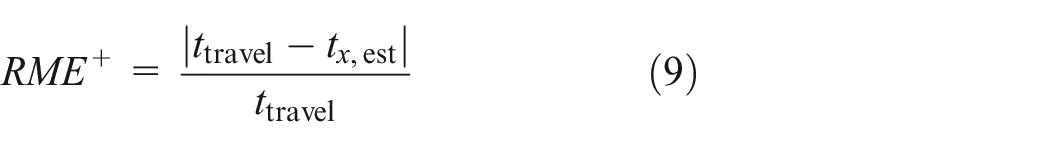
where
5. Evaluation
In this section, we present key findings from the experiments described previously. First, the results of the comparative study for three road segments are laid out in section 5.1. Then, in section 5.2, we demonstrate how travel time estimates can be used to assess the performance of TSE metrics globally. Finally, the results of both experiments are summarized.
5.1. Comparative study
The results of the initial experiment are visualized in Table 2 and Figure 5. We colored the measures based on the utilized sensor technology. The ground truth is colored in orange; measures from the induction loops are colored in yellow; and measures retrieved from FCD are colored in purple. Furthermore, we focus on the hours between 6 am and 10 pm, as during the night hours the network is only sparsely populated and traffic measurements become spotty and less relevant.
Measured mean speeds in km/h for the inspected roads, averaged from 6 am to 10 pm.
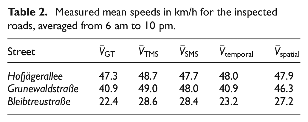
It is apparent that depending on the road type (compare Table 1) the different mean speeds respond differently. On the segment of the Hofjägerallee where there are no traffic lights, at the end of the edge all measures behave similarly. This is due to the highway-like properties of the road. Nearly constant free-flow speeds can be assumed, along the entirety of the edge on all lanes.
On the segments of the Grunewaldstraße and Bleibtreustraße, a clear split in the measures can be noticed. While the time, space, and spatial mean speeds remain close to the speed limit, the ground truth and temporal mean speeds drop to around 40
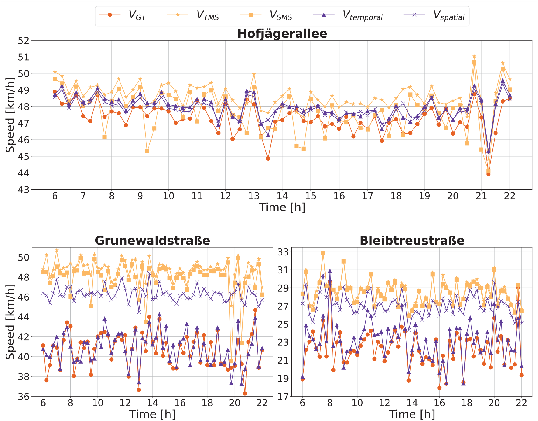
We can also observe that the baseline speeds extracted from SUMO deliver the lowest estimates. As described previously, SUMO extracts the space mean speed, which is biased toward slower vehicles. In contrast, the space mean speed estimation from the induction loops delivers a clear overestimate, due to being unable to capture the entire edge, demonstrating a shortcoming of induction loop sensors for the application of urban TSE. In general, induction loops provided accurate speed measurements on Hofjägerallee but performed less satisfactorily on Grunewaldstraße and Bleibtreustraße. This is due to the limitations of induction loops in capturing urban traffic variability, frequent stops and starts caused by signals and crossings, and their limited spatial coverage missing significant portions of the traffic flow, especially in complex areas. FCD-based speed estimates, on the contrary, are more versatile in covering the entire lengths of streets, but require a certain threshold of participants to provide reliable results. In an attempt to highlight the impact of the penetration rate in FCD-based systems, we ran the same scenario with different ratios of 5%, 10%, 30%, and 100% equipped CVs. For this experiment, we solely looked at the temporal mean speed (
It is evident that the road type and thereby the amount of recorded traversal have a large impact on estimation quality. On the Hofjägerallee, even with penetration rates as low as 5% decent estimation is still possible. The Grunewaldstraße, on the contrary, seems to reach its threshold between 10% and 5% with more outliers and unsampled intervals. Compared with that, the system fails to collect enough samples on the Bleibtreustraße to get a meaningful speed estimate even at penetration rates around 30%. The acquired estimates at market penetrations of 10% and 5% are only sparsely usable. On the Hofjägerallee and the Grunewaldstraße, the number of outliers increases with decreasing penetration rates, and even at 10% we start to see outliers with a significant magnitude.
Initially, we cited penetration rate thresholds of 5%–10% for highway speed estimation. These thresholds only apply to the Hofjägerallee, due to its highway-like characteristics. On the other two streets, measures based on basic FCD reach their limit sooner.
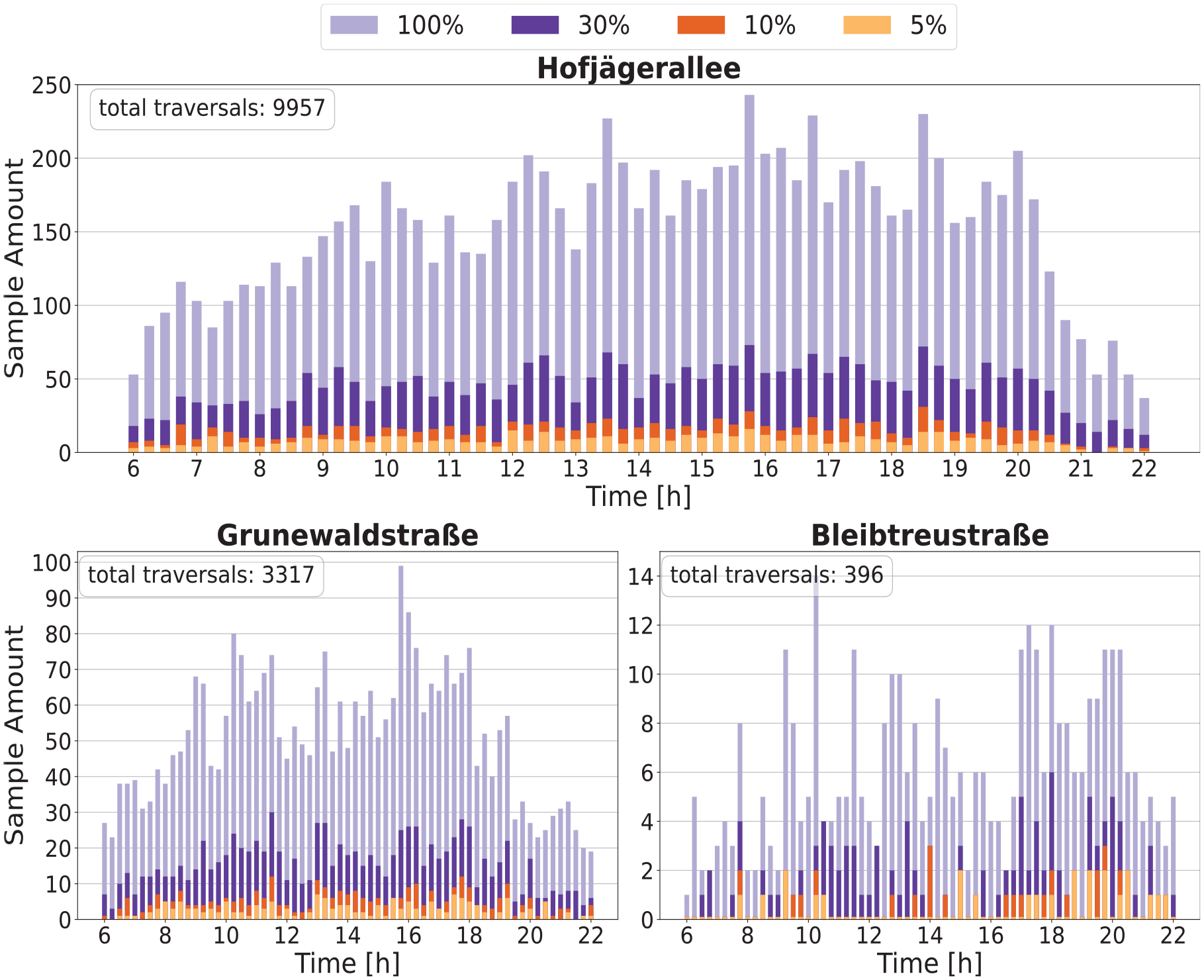
Figure 7 offers more detailed insights into why a meaningful speed estimation might not be possible at lower penetration rates. Here, we look at the number of traversals recorded at the server. The Hofjägerallee and the Grunewaldstraße are traversed thousands of times throughout the day. On the contrary, the Bleibtreustraße is only traversed 400 times, with intervals where merely two traversals are recorded. This makes it highly unlikely for a CV to traverse the Bleibtreustraße even at penetration rates as high as 30%. Usually, as roads like the Bleibtreustraße don’t experience large traffic volumes anyway, less frequent samples aren’t influential. Yet, for use cases like incident detection consistent sampling becomes more relevant.
5.2. Travel time analysis
Finally, we evaluate the estimation results gathered from the travel time analysis. Since the travel time estimation requires insights into a large percentage of the road network, the mean speed measures gathered from induction loops do not suffice. Instead, we again solely focus on the temporal mean speed. For this evaluation, we again equally segmented the time, and considered all vehicles starting their tour within a given interval. In addition, in opposition to previous plots, we also consider times before 6 am and after 10 pm.
Initial results for the previously described
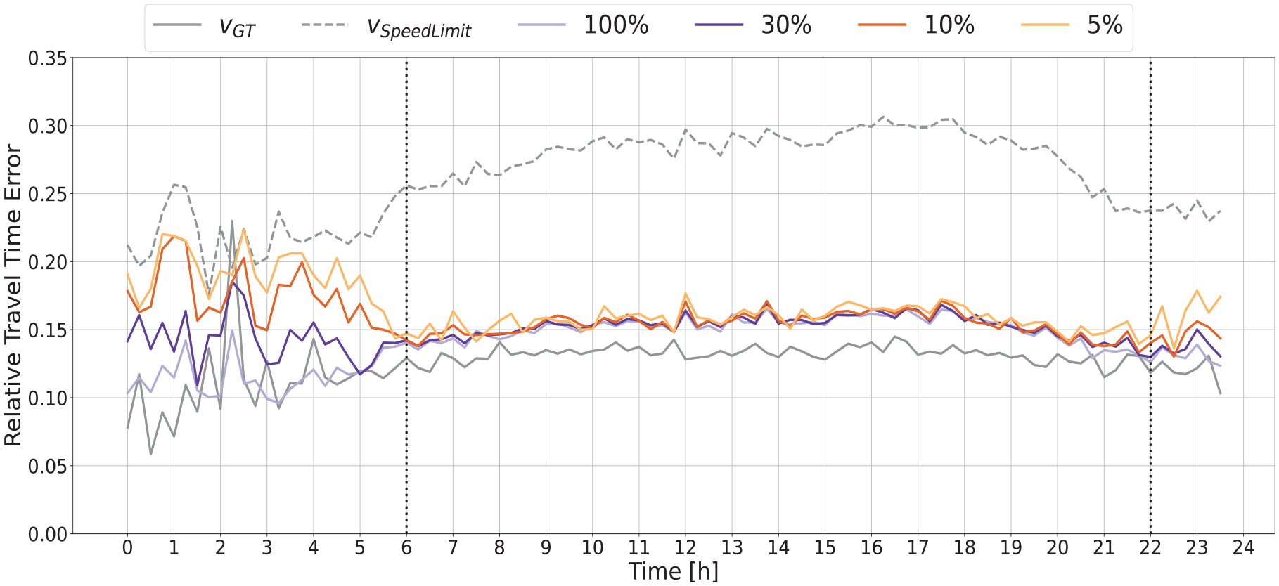
The average relative errors between estimated and actual travel times for different penetration rates using the temporal mean speed.
Nonetheless, significant observations can be made. The travel time estimates based on the ground truth and the ones based on the speed limit seem to form a lower and an upper bound, respectively. Furthermore, before morning and after evening rush hours, it can be observed that even the speed limit as input value suffices to properly estimate travel times within a margin of error of around 15%–25%. However, during the day, when more traffic occurs, the speed limit becomes worse of an input as free-flow speeds are less likely to be reached.
Next, looking at the effect of the penetration rate, again a dependency on the time of day can be seen. In the early morning and late evening hours, higher penetration rates almost strictly lead to better travel time estimations, as only very little traffic is being captured by the FCD, resulting in larger errors for smaller penetration rates. In opposition, during the day, smaller penetration rates still seem to capture enough speed estimates throughout the road network to achieve meaningful estimates. Even at penetration rates as low as 5%, estimates do not seem to suffer from a lack of collected samples, likely because most of the mileage is driven on well-traversed roads, which do not suffer from lower penetration rates as much. Mitigating the general bias, e.g. by integrating turn costs and further information about the road network, would allow for a more fine-grained analysis. Nonetheless, the travel time is suited as a global evaluation metric for TSE quality, especially when lesser populated time periods are considered.
5.3. Summary
To summarize the results, we demonstrated that the published application suite for MOSAIC can act as the basis for a simulative assessment of TSE systems, delivering expected results for implemented metrics. We found that on large, heavily frequented roads (e.g., Hofjägerstraße, and highways) loop detectors can deliver decent results and might be worth the investments. However, on these roads, similar results can be achieved even with a low market penetration of CVs. Speed estimation on highly frequented, signalized urban street segments is more difficult as speeds fluctuate between and within traversals. Single loop detectors fail to produce proper speed estimations, while an FCD-based solution can still closely reconstruct the actual mean speed on those edges. On smaller, less frequented edges both loop detectors as well FCD-based approaches face difficulties. Despite that, even small amounts of FCD can give an insight into the traffic state throughout the day, while no traffic agency would consider loop detector installation on such roads due to costs. Consequently, for smaller roads, the relevancy of a constantly available TSE has to be considered. For these roads, little traffic is expected anyway and obstructions are rare. For this reason, it is possible to drive at the speed limit most of the time and information about the traffic state is not required. However, if a major incident happens even on a smaller road, users would expect a timely reaction by the TSE system to circumnavigate the afflicted area.
Furthermore, we introduced a travel-time-based approach to globally assess the performance of TSE metrics. This metric is suited to compare different speed estimates across different penetration rates on a broad scale. Specifically, the temporal mean speed delivers decent travel time estimates even still at a 5% penetration rate. However, further reduction of the market penetration might worsen these estimates, as indicated by the performance outside of rush hours.
6. Conclusion and outlook
In this paper, we initially offered a review of existing speed metrics for TSE and categorized the challenges one faces when considering complex urban environments compared with highways. Due to much larger fluctuations in individual vehicle behavior, metrics have to be chosen more carefully and potentially from multiple sensor sources for urban applications.
Nonetheless, mean speed estimations always offer insights about the traffic state and are highly important for urban TSE. We identified different commonly used sensor modalities, which lead to different mean speed measures, as different assumptions have to be made when aggregating lossy data from sensors. We classified the Time Mean Speed and the Space Mean Speed as common derivations when dealing with induction loop data. More recent applications based on FCD often rely on curve-fitted approaches, for which we identified the Temporal Mean Speed and Spatial Mean Speed, derived from the work of Yoon et al. 17
To empirically test these measures, we pursued a simulation approach utilizing the strengths of Eclipse MOSAIC. 18 We developed an open-source MOSAIC application suite to calculate the aforementioned mean speed metrics for any traffic scenario. The code for these applications is published on GitHub, 6 together with configuration files for a simulation setup within the Charlottenburg area of the BeST scenario. 7
Based on the published resources, we conducted a comparative study with urban traffic demand provided by the BeST scenario. We found that inner city speed estimations are dependent on the road that they are measured on. The length, speed limit, lane amount, and traffic signals heavily influence the magnitude of realizable speeds as well as the variability. Time and space mean speed measured by single loop detectors often fail to capture the latter, as these are limited to a single observation point.
We showed that FCD-based approaches like the temporal and spatial mean speed are better at capturing the characteristics of entire road segments. As FCD-based systems rely on vehicles as mobile sensors, the equipment rate has to be considered. Our study showed that at rates lower than 15% only partial observations can be made, especially on smaller roads. In the future, we aim to tackle this research question by enriching the FCD set to improve the data quality and enable smaller fleets to provide a sensible TSE. Concisely, we aim to utilize additional information from perception sensors.
In an effort to find a global assessment metric of TSE quality, we introduced a procedure to utilize travel time estimates to evaluate the performance of different metrics throughout the day. We found that even ground truth speed estimates do not yield perfect travel time estimations in part due to the stochastic nature of traffic. Furthermore, we identified that the temporal mean speed, while worse than the ground truth, delivers reliable travel time estimates even at penetration rates as low as 5%. In the future, this evaluation can be used as a reference for novel metrics with considerations of even lower rates of market penetration. In addition, we aim to construct and study scenarios with disruptive traffic patterns (e.g., incidents, second-row parking, etc.) in more detail as these are often most relevant for road users and should be detected by any form of TSE.
Footnotes
Funding
This research received no specific grant from any funding agency in the public, commercial, or not-for-profit sectors.