Sage Journals: Discover world-class research

Abstract

Extraordinary amounts of fresh produce are never purchased and are discarded as waste. Reinforcement learning (RL) could serve as a means to improve business profits while reducing food waste via control of store pricing and ordering decisions. We present a discrete-event-based simulation framework for food retail which simulates wholesaler, store, and customer interactions. This simulator is critical for driving development and testing of future RL methods. It provides an efficient learning feedback system across a wide gamut of possible scenarios, which cannot be replicated from live observations or pure historical data alone. This is crucial as RL agents cannot learn robust decision-making policies without exposure to many unique scenarios. We evaluate our simulator on a demonstrative case generated from historical consumption and price data using a provided methodology for synthesizing daily demand from monthly and yearly stats. In this demonstrative case, we investigate proximal policy optimization, soft actor–critic, and deep Q networks trained with different reward formulations to decrease food waste and improve profits. These RL methods reduced food waste by 78%–92% on average on an unseen 3-year test period as compared to a baseline mimicking typical food retail waste. Compared to a second popular baseline in literature, the best performing RL algorithm was able to improve profits by up to 12.3%.

Keywords

Discrete event simulation reinforcement learning demand function food retail food waste

1. Introduction

Today, more than US$1 T or one-third of all food is thrown away. According to expert estimates measured as the difference between inventory delivered and inventory sold, nearly 40% of fresh products are wasted by most food retail stores.¹ Such waste is neither environmentally conscious nor sustainable, and even worse, it suggests an extraordinarily large wasted potential access to nutrition for those in need. From a business perspective, food waste negatively affects business profits and contributes to extremely tight profit margins (2.2% industry average for food retailers). Reducing food waste presents a significant opportunity toward a more sustainable future and has economic incentives for businesses.

Recent advancements in artificial intelligence (AI) offer new solutions to big societal challenges. As a motivating example, reinforcement learning (RL) methods have managed to greatly outperform expert human decision-making in complex strategic games, such as chess and Go while revealing previously unknown conceptually novel strategies.²Our long-term vision is to exploit RL techniques to optimize food retail operations by reducing food waste while simultaneously improving business profitability.

In food retail, consumer habits and purchasing decisions are highly influenced by various factors, including discounts, weather, seasonality, and product quality. To be profitable, a retailer makes difficult decisions when determining sale price and order/restock quantities of perishable products. Extreme discounts or insufficient orders may result in products running out-of-stock, which presents a loss in potential revenue for retailers. Therefore, overstocking of perishable products is a common business practice to prevent lost sales in the face of variable customer demand, despite the accompanying food waste. As retailers maintain significant markups compared to wholesale prices, the revenue from one product sold to consumers can often cover the loss from more than one product of waste.

Optimal replenishment policies are complex, and simple decision rules cannot be written to cover all constantly changing circumstances. This motivates looking into approximate methods.

A primary hypothesis of our paper is that an RL-driven decision-making system can greatly improve sustainability and retail profitability by decreasing food waste while avoiding understocked inventory. However, for successful application, such a system needs to provide reliable business decisions and autonomously adapt to changing environments. In particular, it must be capable of operating and reacting effectively to both expected events (e.g., holiday season) and unexpected events (e.g., pandemic, drought, and new health trend). Both types of events can affect wholesale prices of products, and consumer purchase behaviors.

Consequently, any intelligent RL system requires rigorous evaluation on a wide gamut of possible events prior to deployment in a real environment. As historical data limit the examples an RL system can learn from, simulation plays a crucial role for training and evaluating RL-based decision-making systems. Such simulation must be capable of not only properly evaluating state transitions but also be able to generate high-quality examples of situations which can be, but have not been, encountered in real prior data.

Problem statement. Adapting RL to reduce food waste and improve profitability in food retail stores requires a learning and testing environment where a myriad of events can be learned from and relevant data can be accessed. Unfortunately, existing simulators, e.g., work by Teller et al.³ and Baydar⁴ (Section 2.2), fail to provide interfaces to food waste, product deliveries, purchase tracking, and pricing/ordering control, which is a prerequisite for an RL approach in food retail.

Objectives. This paper aims to provide intelligent decision-making in food retail to reduce food waste and maintain profitability by innovatively combining RL with simulation techniques. In particular, our paper aims to (1) provide a simulation framework that can be used for the development, validation, and testing of RL methods. It also (2) offers realistic, product-specific demand functions to estimate expected purchases. Moreover, (3) the paper provides a detailed experimental evaluation of various RL algorithms in a food retail context using our simulator and demand functions.

Contributions. Our research presents novel technical contributions in the following areas:

A food retail simulator capable of simulating a food retail environment with event, seasonal, and day-to-day demand variations, revenue, food spoilage (waste), product deliveries, and product pricing.

Synthesis of realistic demand from historical data and statistics for training and testing RL agents.

Conceptual methodology for applying RL to the retail food waste problem via simulation.

Detailed experimental evaluation for strawberries, potatoes, and carrots derived from historical data compared to two baseline approaches.

This paper extends our previous work⁵ by providing more realistic demand functions (Section 5), applying additional RL algorithms (Section 4.2) and carrying out a more extensive experimental evaluation (Section 6) with three perishable food products and two baseline algorithms. In addition, the formal background of RL algorithms and related work is also discussed more extensively in this article.

Significance. A highly customizable food retail simulator provides a sandbox environment to develop and test RL solutions for optimizing pricing and inventory management of perishable items. It allows an RL agent to experience, experiment, and learn from an immense number of unique realities and events which have not occurred, rather than being restricted to limited live and historical data. A methodology for generating realistic demand functions enables the application of AI techniques even for stores which have limited historical data. Furthermore, it contributes a conceptual methodology for RL application to reduce food spoilage and waste in food retail practices.

2. Background and related work

2.1. Background

Decisions in food retail stores. Successful store management requires careful decision-making to maintain profitability in a low profit margin environment. In this endeavor, food retail stores have many strategies, including adjusting product arrangement and organization to drive customer traffic to certain products within a store. However, fundamentally, the key decisions a store makes are (a) what price to set for products and (b) how many products to order from wholesale to stock inventories. These decisions are not completely independent and directly affect profits. For example, changes in product price can impact customer demand, which then requires a change in order quantity. When there is excess inventory, product discounts may be needed to avoid large sunk costs due to food waste.

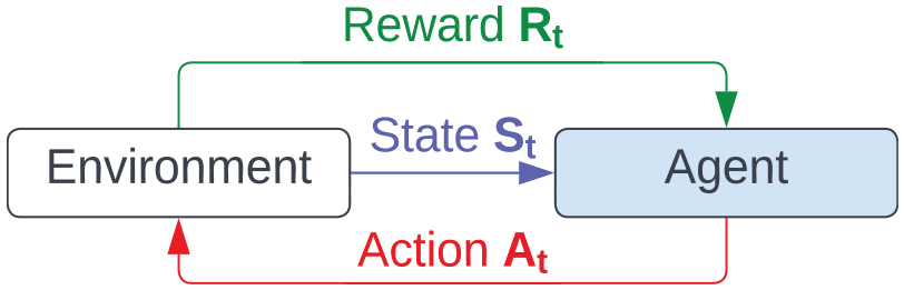
Discrete Event Simulation. $DES = (Σ, Ev)$ models the behavior of a system with a set of states $Σ$ (value assignments to state variables) and a set of discrete (instantaneous) events $Ev$ . When an event occurs $e_{t_{i}}$ at time $t_{i}$ , the state trajectory $Σ (t_{i})$ of the system is changed (updated state variables), and the simulation time is set to $t_{i}$ . The state of the system remains stable until when the next event $e_{t_{i + 1}}^{'}$ occurs at time $t_{i + 1}$ . We intentionally keep this DES definition at a high level of abstraction, but note that RL could also be integrated with other simulation formalisms (e.g., discrete event system specification (DEVS))⁶ for smart retail optimization.

Reinforcement learning. RL is a machine learning technique which seeks to learn what actions to perform in a given situation via feedback from rewards. RL problems can be represented by Markov Decision Processes $MDP = (S, A, R, T); π : S \to A$ (shown in Figure 1). An RL agent interacts with its environment.⁷ At discrete moments of time, $t, t + 1, \dots$ , the agent observes an environment state $S_{t}$ . The agent determines what action $A_{t}$ to perform as the next decision. This action changes the state of the system $S_{t}$ to $S_{t + 1}$ according to a probabilistic state transition function $T$ . At any time $t$ , the agent may receive a reward $R_{t}$ , which is used as feedback to learn better action strategies. Formally, an action strategy is called a policy $π (a | s)$ which determines an action $a$ for a given state $s$ . The agent learns along episodes consisting of a sequence of states $S_{0}, S_{1}, \dots, S_{n}$ ending on a terminal state $S_{n}$ (e.g., playing a game). Most RL techniques require significant numbers of episodes to learn effective policies. In most cases, the agent does not know the state but rather is limited to observations. Literature generally refers to this setup as a Partially Observable Markov Decision Process, POMDP. A non-exhaustive list of RL algorithm types includes multi-armed bandit, actor–critic, and Q-learning.⁷ Each has its benefits and disadvantages. Finding effective RL solutions for challenging real-world problems may require experimentation with many algorithm types.

Figure 1.

RL formulation.⁵

In an RL setting, pricing and ordering decisions can be mapped to agent actions. The state of the environment can encapsulate information, such as the season and number of products in inventory. With a carefully crafted (custom) reward function and sufficient learning episodes (e.g., via simulation), an RL agent could learn a pricing policy and ordering policy used in given environment states.

Value functions in RL. Many RL algorithms seek to learn the value of particular states or state–action pairs. Intuitively, by approximately learning the value of particular states, the algorithm can also learn a policy (strategy) for actions to lead the agent to high-value states.

Soft Actor–Critic. Soft actor–critic (SAC) is an RL algorithm which seeks to maximize both cumulative reward and its policy’s entropy (or stochasticity).⁸ It is a deep RL algorithm which uses three neural networks to learn three functions. The original SAC formulation used these three neural networks to learn a state value function (approximates cumulative future rewards starting at state $s_{t}$ ) $V (s_{t})$ , a soft Q state–action pair value function $Q_{Θ} (s_{t}, a_{t})$ approximates the long-term reward of a state–action pair, and a policy function $π_{θ} (a_{t} | s_{t})$ . The policy function provides an action given a state. Each function is parameterized by its own neural network (e.g., $θ$ or $Θ$ ) with accompanying weights and biases. Modern iterations (such as in the Stable Baselines3 library by Raffin et al.⁹) replace the state value function with another soft Q state–action pair value function as the value function can be parameterized through Q-function parameters, $V (s_{t}, a_{t}) = E_{a_{t} ~ π} [Q (s_{t}, a_{t}) - α π (a_{t} | s_{t})]$ . The soft Q-functions are learned by minimizing the loss $J_{Q} (Θ) = E_{(s_{t}, a_{t}) ~ D} [\frac{1}{2} {(Q_{Θ} (s_{t}, a_{t}) - (r (s_{t}, a_{t}), + γ E_{s_{t + 1} ~ T} [V_{\bar{Θ}} (s_{t + 1})]))}^{2}]$ . Here, $r (s_{t}, a_{t})$ is the reward received from performing action $a_{t}$ and state $s_{t}$ . The policy function is learned by minimizing the following loss function: $J_{π} (θ) = E_{s_{t} ~ D} [α (π_{θ} (a_{t} | s_{t})) - Q_{Θ} (s_{t}, a_{t})]$ . $α$ is a learning rate hyperparameter and $γ$ is a discount factor used to balance future and immediate rewards. These hyperparameters must be set manually/experimented with to see what works best.

Proximal Policy Optimization. Proximal policy optimization (PPO) is a policy gradient method RL algorithm that maintains two policy neural networks. One designates the policy we are trying to refine and the other is the policy we last used to collect samples via actions in the environment. PPO minimizes its cost function through small update steps that avoid diverging its new policy too far from the previous policy.¹⁰ PPO improves on trust region policy optimization (TRPO)¹¹ through a clipped surrogate objective, $L^{CLIP} (θ) = {\hat{E}}_{t} [\min (r_{t} (θ)^A_{t}, clip (r_{t} (θ), 1 - ϵ, 1 + ϵ)^A_{t})]$ where the probability ratio is $r_{t} (θ) = \frac{π_{θ} (a_{t} | s_{t})}{π_{θ_{old}} (a_{t} | s_{t})}$ and $^A_{t}$ is the estimator of the advantage function at timestep t. The advantage function finds the relative value for a selected action. $ϵ$ is just some clipping parameter, e.g., can be set to 0.2. This new clipped objective function aims to select the minimum between the original TRPO objective, ${\hat{E}}_{t} [r_{t} (θ)^A_{t}]$ , and a clipped version of this objective around some $ϵ$ . With this change, the unclipped objective is used whenever the clipped objective fails to improve the overall objective.

Deep Q-learning. Deep Q-learning (DQN) is a Q-learning approach which improves on original table-based representations of the Q-function by employing a parameterizable neural network instead¹² (same as in SAC). The neural network acts as a non-linear function approximator of the Q-function, where $θ$ is the parameter of the network.¹² DQN is also a model-free, off-policy approach that uses a behavior distribution, $ρ$ , to explore the environment and minimize loss through $L_{i} (θ_{i}) = E_{(s, a) ~ ρ (\cdot)} [(y_{i} - Q {(s, a; θ_{i})}^{2}]$ , where $y_{i}$ is the target value represented by $y_{i} = E_{(s^{'} ~ ε} [r + γ_{a^{'}} Q (s^{'}, a^{'}; θ_{i - 1}) | s, a]$ . $γ$ is a discount factor. After each timestep, $θ$ is updated using stochastic gradient descent.

2.2. Related work

Related work spans the research fields of simulation and machine learning, and includes literature on sales forecasting,¹³ price optimization,¹⁴ customer behavior,¹⁵ food waste,³ and inventory restock policy.^16,17 Our work differentiates itself from existing work by simulating a food retail environment in which RL-driven store management is possible. Moreover, most existing simulators are either (a) not available off-the-shelf or (b) cannot be tailored to the needs of food waste reduction of individual retail stores as they lack sufficient customizability to simulate specific product definitions, prices, and relevant entities. Furthermore, we conduct a food retail demonstrative case with RL techniques and reward formulations not previously explored in the food retail domain.

Simulation. Baydar⁴ creates an agent-based simulation environment for a grocery store and uses optimization to determine discount amounts for particular customers to balance pricing, sales volume, and customer satisfaction. While this is a similar work discovered in our literature search, it does not factor in wholesalers, control over delivery order sizes, nor model food waste.¹⁸ However, develop a single-store simulator for food waste relying on the Poisson distribution. This simulation is limited to need-based purchases. Customers always select the cheapest product available that meets their remaining days of freshness requirement. Welling et al.¹⁹ provide a discrete event simulator by following the 12-step simulation development process to study lead-time-based pricing for semiconductor supply chains. Lau et al.²⁰ create a simulator studying the effects of inventory policy on supply chain performance with four retailers and one supplier. This simulator generates random demand and production capacities, and models retailer and supplier decisions. Christensen et al.²¹ propose forecasting methods using product shelf life and validate these methods through simple simulation. To evaluate the effect of price management on food retail,¹⁸ build a simulation of food retailers.

Customer behavior. Customer behavior focuses on understanding how an individual customer interacts with—stores, products, and brands—and applies a model to predict future actions. Initial examinations of modeling consumer purchase behavior as Stochastic Processes in the work by Rao²² and Aaker and Jones²³ state that customer purchase behavior is stringent and not easily changed (store and brand loyalty). However, various simulations analyze when to centralize and decentralize groups of customers, as an example, through geographical information.^13,24 In e-commerce platforms, constraints and additional insights are often provided to help model future customer actions. Such models handle customer behavior as a multivariate multinomial problem or a hidden Markov model.^15,25

Perishable inventory management and pricing. There is a set of relevant literature in the perishable inventory management and pricing field. Nahmias²⁶, Raafat²⁷, and Goyal and Giri²⁸ provide reviews and surveys of the field. Relevant work includes the work of Goto et al.²⁹ who study the optimal ordering policy for the airline meal by Markov decision processes. Chen et al.³⁰ and Jia and Hu³¹ both investigate pricing and ordering decisions for a retailer and supplier operating on perishable products. Other relevant literature includes the work of Broekmeulen and Van Donselaar³² who develop a new replenishment policy which calculates and uses the age of inventories, and compares with a baseline which does not. This same baseline is used in the work by Tekin and Gürler Berk³³ who likewise investigate reorder control policy for perishable products.

Reinforcement learning. Rolf et al.³⁴ provide an extensive review of RL methods and algorithms used within the supply chain contexts, including perishable food items. For example, Chen et al.³⁵ develop a deep learning RL method for agri-food supply chain profit optimization. Afridi et al.³⁶ use simulation to develop and test a deep Q-learning-based approach to replenishment policy in vendor management inventory for semiconductors which leads to significant improvements over a baseline. Similarly, Oroojlooyjadid et al.³⁷ use simulation and a Q-learning-based approach for the inventory optimization problem to achieve near optimal order quantities in the beer game. Chaharsooghi et al.³⁸ investigate many players in the beer game supply chain controlled via multi-agent RL. Gijsbrechts et al.³⁹ adapt A3C deep RL for inventory management problems and match state-of-the-art heuristic and dynamic programming solutions in simulation. Finally, David and Syriani⁴⁰ propose the use of RL techniques to create DEVS models.

RL in perishable retail. Some related works regarding RL focus on perishable retail. Kara and Dogan⁴¹ experiment with Q-learning and SARSA for waste reduction. Sun et al.⁴² found that DQN can reduce the amount of spoilage for fresh product retailers. A recent work by Jullien et al.⁴³ approaches the food waste problem with RL and introduces a new algorithm. Our work differentiates itself by (1) building a more customizable multi-entity simulation framework, (2) developing a new methodology for demand synthesization, and (3) investigating a new demonstrative case and reward function.

3. A food retail simulator

3.1. Architecture of food retail simulator

Our discrete event simulation (DES) framework allows for RL-driven control of individual store decision-making. The user inputs stores, wholesalers, and (groups of) customers definitions and behavioral functions to initialize the simulation environment. Ideally, underlying demand functions governing customer purchase behavior are based on real food retail data (Section 5). The simulation models entity interactions on a day-by-day basis and keeps track of sequences of events.

Simulation architecture. The detailed simulation architecture and how it maps into an RL problem space can be seen in Figure 2. A store interacts with its environment and can be controlled by an RL agent. This agent performs actions given information received from the environment. Such information is provided in the form of events (e.g., a product purchase or spoilage). Such events (marked in blue) designate updates in the environmental state and store observation. Pricing and order decisions (red) can be considered as RL actions (e.g., set the product price). The environment controls when a store can perform an action. When it is the time for the agent to perform an action, an observation of the state is constructed from prior event information. The action is passed as a pricing or order event to the environment, which properly handles the outcome. These constitute observable events which the simulator can log, record, and save. Information encoded within events can be used to form (green) rewards (e.g., a measure combining profit and food waste).

Figure 2.

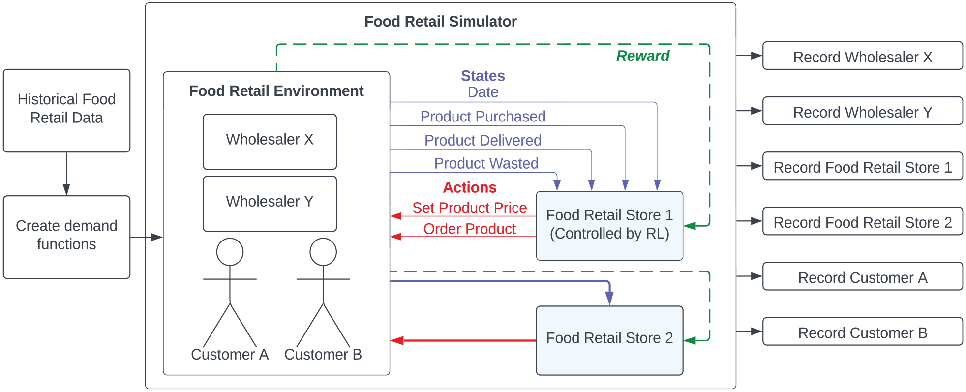
Simulator architecture with state information colored in blue, actions in red, and rewards in green.⁵

By design, we specifically avoid imposing any concrete RL formulation for our targeted retail food waste problem. This prevents our solution space from being restricted to a particular definition of a reward or state representation.

As an abstraction, the simulator passes events from which rewards and observations can be formed. This highly flexible abstractions allow for experimentation with any class of RL technique (or alternative approaches) and different reward/observation definitions. The potential solution space for the food retail waste problem is expansive with many valid RL problem formulations. We present a demonstrative case with several RL algorithms and products in Section 4.

Food retail environment. Our simulation environment follows a DES framework where time increments in (discrete) daily intervals. We provide three primitive entity types. (1) Wholesalers sell products to stores. They control the price at which they sell a particular quantity of products on a particular day. (2) Stores purchase products from wholesalers for their inventory which customers can then buy. Stores set the prices at which to sell products to customers and when to order additional products from wholesalers. (3) Customers purchase products from stores. A customer may be an individual or a group of customers with similar purchasing behavior.

Each entity has its own underlying control function (e.g., RL in Section 3.1) which makes decisions (e.g., pricing, purchasing, and ordering) on a daily basis subject to potential constraints. The control function could be abstracted to subfunctions for individual products or aggregated to cover all products at once. As entities interact, each entity’s actions produce events which alter the state of the environment. For example, environment state changes may manifest as changes in store inventory values or food wasted.

Each entity may have defined constraints on its decision (action) space. Such constraints could include maximum price increases for designated products or limits on what days the entity can submit restock orders. This is highly configurable. For example, in Section 4, we limit restocking orders to two weekdays and prices to weekly adjustment.

Each event generated via interaction between wholesaler, store, and customer entities is well defined and appropriately consumed to trigger potential state transitions. For example, a customer purchasing a product from a store produces a purchase event which triggers a change in inventory. Generated events are validated on the fly via type and instance checking.

3.2. Methodology of food retail simulator

Simulation allows for the training and testing of RL agents across a myriad of expected and unexpected food retail events. Effective simulation must be computationally efficient and customizable. Furthermore, generated data and statistics must be safely accessible. Our simulator captures the food retail environment, correctly generates states, and acts accordingly to actions undertaken by store-controlling RL agents.

Configuration. To configure the simulation, the user defines the simulation start and end dates, the number of episodes to perform, and the number of parallel threads to use. The base configuration file (in TOML format) also supplies links to product, wholesaler, store, and customer entity definitions, their relations, and their behavior control functions. The base configuration file can serve as documentation for future simulation reruns or extensions.

DES environment for food retail. Simulation (Algorithm 1) follows a daily pattern with each day consisting of a sequence of discrete events which signal environment state changes. Six primary event types are produced and consumed:

PriceSetEvent is generated when a store agent changes the price of a product.

ProductOrderedEvent is created when a store agent places an order to a wholesaler.

ProductSoldEvent occurs from a customer purchase. The product is removed from inventory.

ProductDeliveredEvent alerts that a delivery from a wholesaler has arrived. Product added.

ProductWastedEvent is triggered when a product has reached its expiration date. Product removed.

EODEvent marks the end of the day. The date is moved forward by one day.

Algorithm 1: Simulate Day (Pilarski et al.⁵)
Input: date, wholesalers, stores, deliveries, customers Output: eventLog 1 foreachstore in stores do 2 foreachdelivery in deliveries[store] do 3 de = newProductDeliveredEvent(date, store, delivery.wholesaler, delivery.product) 4 store.update(de); // add delivered products to inventory 5 eventLog.append(de) 6 foreachep in store.expiringProducts do 7 we = newProductWastedEvent(date, store, ep) 8 store.update(we); // expired products are removed 9 eventLog.append(we) 10 orderActions = store.getOrderActions() 11 foreachoAct in orderActions do 12 oe = newProductOrderedEvent(date, store, oAct.wholesaler, oAct.prodType, oAct.orderPrice) 13 wholesaler.update(oe); // fulfill product order 14 store.update(oe); // product order confirmation 15 eventLog.append(oe) 16 priceActions = store.getPriceActions() 17 foreachpAct in priceActions do 18 pe = newPriceSetEvent(date, store, pAct.product, pAct.price) 19 store.update(pe); // change price of product in store 20 eventLog.append(pe) 21 whilecustomers not done shopping do 22 customer = select from customers 23 purchase = customer.shop() 24 se = newProductSoldEvent(purchase.store, purchase.product, purchase.price) 25 purchase.store.update(se); // remove product from inventory 26 eventLog.append(se) 27 eod = newEODEvent(date) 28 foreachentity in (wholesalers, stores, customers, deliveries) do 29 entity.update(eod); // next day starts 30 eventLog.append(eod); 31 return eventLog

Algorithm 1: Simulate Day (Pilarski et al.⁵)

Input: date, wholesalers, stores, deliveries, customers
Output: eventLog
1 foreachstore in stores do
2 foreachdelivery in deliveries[store] do
3 de = newProductDeliveredEvent(date, store,
delivery.wholesaler, delivery.product)
4 store.update(de);
// add delivered products to inventory
5 eventLog.append(de)
6 foreachep in store.expiringProducts do
7 we = newProductWastedEvent(date, store, ep)
8 store.update(we);
// expired products are removed
9 eventLog.append(we)
10 orderActions = store.getOrderActions()
11 foreachoAct in orderActions do
12 oe = newProductOrderedEvent(date, store,
oAct.wholesaler, oAct.prodType, oAct.orderPrice)
13 wholesaler.update(oe);
// fulfill product order
14 store.update(oe);
// product order confirmation
15 eventLog.append(oe)
16 priceActions = store.getPriceActions()
17 foreachpAct in priceActions do
18 pe = newPriceSetEvent(date, store,
pAct.product, pAct.price)
19 store.update(pe);
// change price of product in store
20 eventLog.append(pe)
21 whilecustomers not done shopping do
22 customer = select from customers
23 purchase = customer.shop()
24 se = newProductSoldEvent(purchase.store, purchase.product, purchase.price)
25 purchase.store.update(se);
// remove product from inventory
26 eventLog.append(se)
27 eod = newEODEvent(date)
28 foreachentity in (wholesalers, stores, customers, deliveries) do
29 entity.update(eod);
// next day starts
30 eventLog.append(eod);
31 return eventLog

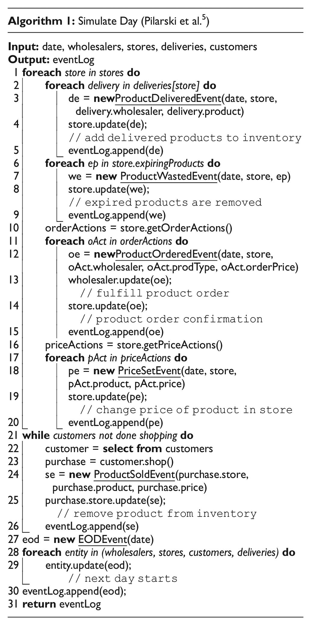
Algorithm 1 shows how a day is simulated. Each day follows a fixed high-level order of events.

The day begins with deliveries (Lines 2–5): a ProductDeliveredEvent is created for an arriving product. The delivered product is added to the store’s inventory using event data.

Next, expiring food is removed from a store’s inventory (Lines 6–9). A ProductWastedEvent is created which provides a link to the store and the expiring product. The store is then updated via this event, wherein it removes the product from its inventory.

The store then has the option to order more products (Lines 10–15). A store’s agent provides a list of order actions it would like to perform. These order actions are then transformed into ProductOrderEvents which update both the wholesaler from which the product is purchased and the store. These updates begin the order and delivery process and confirm to the store that the order was accepted.

Similarly, the store then makes pricing decisions (Lines 16–20). An agent generates a list of price actions. From this list, PriceSetEvents are created to record how the store changes the product price.

At this time, the store becomes open for customers to shop (Lines 21–26). A customer is selected until all customer groups have completed their shopping. This customer determines their next purchase, which then is used to form a ProductSoldEvent. This event is then used to update the store to remove the purchased product from inventory. Such implementation allows randomization of customer orders (e.g., different customers purchasing the last product leads to different behaviors).

Once the customers have completed their shopping, an EODEvent is created to update all entities that the day is over. A new day can then be simulated.

Customer behavior. Modeling customer purchase behavior is critical for food retail simulation. In our simulator, a demand function representing the desired demand for a product (i.e., quantity to purchase at a price) controls customer purchase behavior. The demand function template is flexible and allows for many possible inputs, such as product price, season/date, and product freshness. For simulation realism, it is best if such functions are derived from historical customer demand data. We generate such functions from historical statistics in Section 5.

Logger. Event-driven simulation environment updates have two key benefits: (1) they can provide simulation correctness and consistency guarantees, and (2) events provide a simple schema for logging and tracking simulations and statistics. Our simulator features a logger which calculates statistics across simulations.

Multiprocessing. Simulation runs are independent; thus, they can be parallelized. The simulator allows for multiprocessing simulations across multiple CPU cores or threads for significant simulation speedup. Rewriting the simulator in C++ can provide further runtime improvements.

Simulator design. We followed a DES framework rather than a DEVS framework when designing our simulator, as it sufficiently meets our requirements. Our primary objective is to enable RL control for store pricing and ordering decisions which does not require modeling continuous time. For this purpose, we also developed gymnasium⁴⁴ wrappers to make it easy to experiment with existing algorithms. DES allowed for quicker design, development, and testing of the initial simulator version. Furthermore, it capably handles macro (daily) information which is sufficient for exploring RL for food retail optimization.

In the future, we do plan to extend the simulation environment to a DEVS framework to model more detailed, continuous-time customer behavior (e.g., shopping or delivery at particular hours).

Software as a service deployment of the simulator is possible via a public interface, which could provide smooth integration with existing food retail solutions in the future.

4. Demonstrative case: base assumptions

As a feasibility demonstration and initial evaluation of the simulator, we run a simulation campaign. This campaign implements a synthetic grocery store derived from aggregated real data to demonstrate both how the simulator can be used and to explore some RL problem formulations and potential benefits.

4.1. Simulation scenario

We set up the simulation with the following entities and parameters. (1) One wholesaler, (2) One customer group, and (3) One store which can only order products on Mondays and Thursdays. (4) An agent controls the store-level decision-making regarding the purchase quantity of three perishable products with unique demand patterns and seasonality. The prices of products are set on Mondays, but this is not controlled by the agent.

4.2. Agent assumptions

Observations The range of observations an agent is allowed to access is listed below. We leave these general here, as the way they are implemented can have a significant effect on performance. We provide a detailed observation setup when presenting results in Section 6.

Time can be observed and represented in many ways, including daily, weekly, monthly, with continuous and one-hot-encoding schemes.

Inventory levels for each product at each time can be observed and represented numerically.

Quantities purchased by customers over a period of time can be observed and represented in an aggregated manner.

A Demand forecast for upcoming customer purchase quantities is available to the agent.

Reward Functions RL agents can be trained on various reward formulations. These rewards can be constructed via combinations of:

Sold quantities and monetary values

Order totals and monetary values

Food waste totals and monetary values

Agent Algorithms We evaluate the following algorithms:

PPO.¹⁰ It is an on-policy algorithm which has been shown to learn reliably in literature.

SAC.⁸ This algorithm is a sample-efficient off-policy algorithm which is known to produce good policies.

DQN.¹² This algorithm has been demonstrated to perform well in similar problems.

4.3. Product assumptions

Our simulation study consists of several products which have different seasonality patterns and times to expiration.

Strawberries have a short time to expiration and a consistent summer demand peak.

Carrots have a medium time to expiration and demand is slightly more seasonal throughout the year than potatoes.

Potatoes have a long time to expiration with more constant, yet still variable demand throughout the year.

How daily demand is determined for each of these products is presented in Section 5. We consider these three different product categories for evaluating algorithms across a breadth of perishable product categories.

5. Deriving demand functions for products

This section outlines the data sources and methodology developed to generate daily demand for the demonstrative case in Section 4. As access to high-quality daily historical sales data, we investigate the following research question.

RQ1: How can one generate synthetic, yet realistic daily demand functions from aggregated data that satisfy the following criteria?

- Correctness: Daily demand aggregates to historical monthly and yearly levels for each product.

- Seasonality: Demand follows expected seasonal yearly patterns.

- Diversity: Demand patterns exhibit appropriate variation across years.

5.1. Data sources

To build realistic demand profiles for each product, we rely on the Statista database for historical statistics regarding quantities of strawberries, potatoes, and carrots sold and consumed per month and per year.

We build the potato demand function on data from yearly (2009–2019) potato sales⁴⁵ and monthly sales by month in Spain in 2020.⁴⁶ We use similar yearly and monthly data for strawberries and potatoes as well.^47–50

While we merge data from different countries, all data are from the Northern hemisphere and should exhibit similar seasonal patterns. As there always exists variation in demand for a particular location, any variations between these data sources should not overwhelmingly affect realism.

5.2. Generating daily demand

Our simulation setup (Section 3.1) requires daily demand. However, the data sources are limited to the measures of total demand per year and a monthly demand breakdown for 1 year. Thus, we develop and use an interpolation method to derive daily demand for each product. This method is presented in Algorithm 2.

Algorithm 2: Generate daily demand functions
Input: demandMonthlyStat, demandYearlyStat Output: demandDaily 1 foreachyear in years do 2 // Yearly to Monthly 3 demandMonthlyStatNoisy = addNoise(demandMonthlyStat) 4 estDemandMonthly = demandYearlyStat[year]*demandMonthlyStatNoisy / sum(demandMonthlyStatNoisy) 5 // Finding FOMS 6 FOMS1 = linearInterpolation(estDemandMonthly) 7 FOMS2 = midpointMethod(estDemandMonthly) 8 FOMS = mean(FOMS1, FOMS2) 9 // Cubic Interpolation 10 dailyDemand = cubicInterpolation(FOMS) 11 // SLSQP Optimization 12 dailyDemand = SLSQPMinimize( MonthlyDiff(dailyDemand, estDemandMonthly)) 13 // Customer Foot Traffic 14 dailyDemand = customerFootTrafficShift(dailyDemand) 15 return dailyDemand

Algorithm 2: Generate daily demand functions

Input: demandMonthlyStat, demandYearlyStat
Output: demandDaily
1 foreachyear in years do
2 // Yearly to Monthly
3 demandMonthlyStatNoisy = addNoise(demandMonthlyStat)
4 estDemandMonthly = demandYearlyStat[year]*demandMonthlyStatNoisy / sum(demandMonthlyStatNoisy)
5 // Finding FOMS
6 FOMS1 = linearInterpolation(estDemandMonthly)
7 FOMS2 = midpointMethod(estDemandMonthly)
8 FOMS = mean(FOMS1, FOMS2)
9 // Cubic Interpolation
10 dailyDemand = cubicInterpolation(FOMS)
11 // SLSQP Optimization
12 dailyDemand = SLSQPMinimize( MonthlyDiff(dailyDemand, estDemandMonthly))
13 // Customer Foot Traffic
14 dailyDemand = customerFootTrafficShift(dailyDemand)
15 return dailyDemand

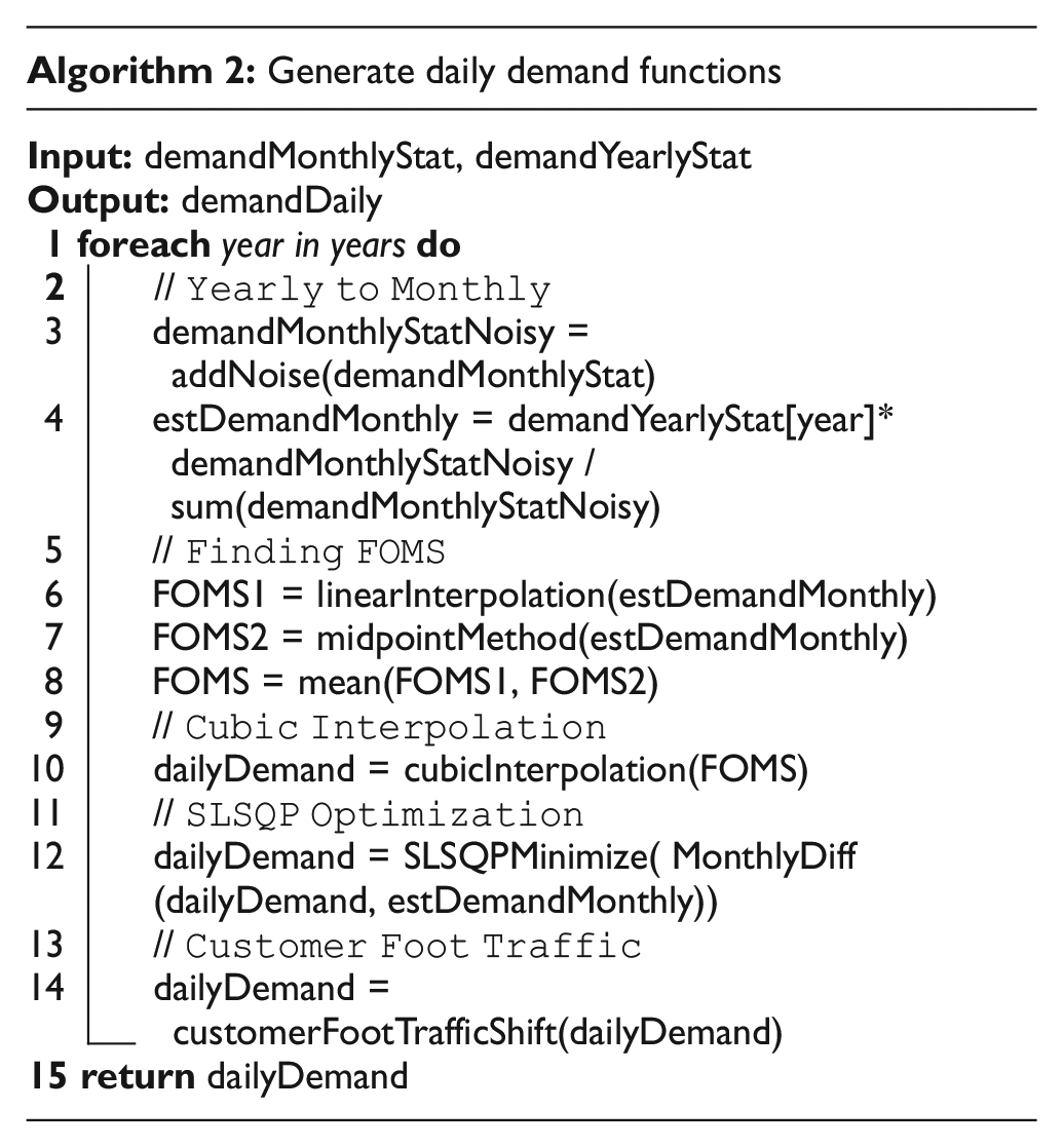
This process is divided into two parts: yearly to monthly and monthly to daily. The first connects yearly demand data points to monthly total sales, and the second uses the monthly totals to infer the corresponding daily demand for that year.

Yearly to monthly. As available monthly demand breakdown statistics are limited to 1 year, expected monthly totals for other simulation years must be generated. This can be accomplished by treating the monthly demand as a weighted demand concentration within the year. Furthermore, one can introduce extra variation between years by injecting random noise into the monthly parameters. In this article, we add noise to each month by sampling from Gaussian noise centered at 0, with a variance of 1/10th the monthly demand value. This maintains the general monthly seasonality shape across years with realistic quantities. This step can be seen in Lines 2–4 of Algorithm 2.

Monthly to daily. Given monthly demand totals for each simulation year, we develop a methodology to convert monthly demand to daily values via interpolation. On a high level, this methodology consists of (1) determining first-of-month sales (FOMS) basis points from the raw data, (2) interpolation to daily values, (3) Sequential Least Squares Programming (SLSQP) optimization to adjust FOMS for interpolation sales to match expected sales, and (4) shifting demand between weekdays based on customer foot traffic.

FOMS. As each monthly total is the sum of discrete daily demand across a month, one can derive a series of basis points corresponding to the FOMS by averaging two distinct approximations. The first approximation (FOMS linear interpolation) uses linear interpolation to generate a system of equations that can be solved using a least-squares approximation. The second approach (FOMS midpoint method) assumes the FOMS of a given month is the midpoint selling volume of the monthly total of the previous and following month, averaged over the total days in the month.

FOMS linear interpolation. This method starts by naively assuming linearly increasing and decreasing demands between FOM dates to get an initial set of basis starting points. This produces a solvable series of linear equations as the sum of demands between the dates can be set equal to the determined total monthly demand. This can be done by setting the FOMS for each month to a variable, e.g., $F_{1}, F_{2}, F_{3} . . .$ . If there are $d$ days between the first days of 2 months, $m_{n}, m_{n + 1}$ , then the total demand (assuming linearity) across the month $m_{n}$ is always $d (F_{n} + F_{n + 1}) / 2$ . This can be intuitively seen in Figure 3 geometrically. The corresponding equations are here as follows:

F_{n} < F_{n + 1} : d \cdot F_{n} + d (F_{n + 1} - F_{n}) / 2 = d (F_{n} + F_{n + 1}) / 2

F_{n} > F_{n + 1} : d \cdot F_{n + 1} + d (F_{n} - F_{n + 1}) / 2 = d (F_{n} + F_{n + 1}) / 2

Figure 3.

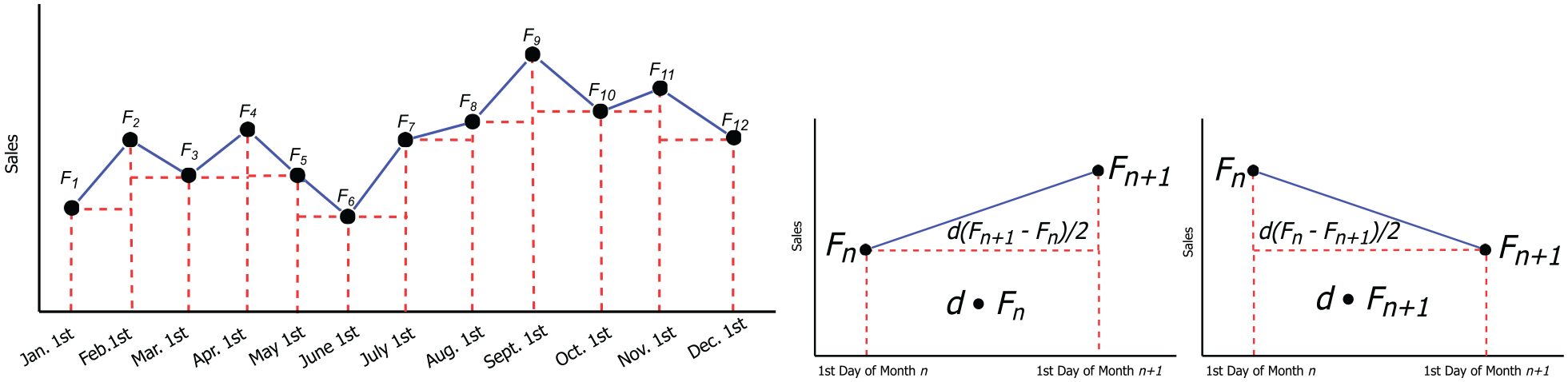
(Left) Linear interpolation between FOMS (Right) and two cases between consecutive points.

The series of equations can be rewritten as a matrix equation. However, this can result in a non-singular matrix, which prevents systematic equation solving. The solution therefore can be approximated by solving the equation via the least-squares method.

FOMS midpoint method. The second approach to finding a FOM demand value is to set it to the mean daily sales across the previous month and the present month.

The final basis points used for upcoming steps are created by finding the average of the linearly determined basis points and the midpoint method. Finding FOMS can be found on Lines 6–8 of Algorithm 2.

Interpolation. Given the set of FOMS basis points, it is possible to interpolate to daily demand. We use cubic interpolation as it preserves the continuity between months, unlike linear and quadratic interpolation, thereby improving realism. As interpolation returns a continuous demand function, each day can be sampled to return daily demand (Line 10 in Algorithm 2).

SLSQP optimization. The cubic interpolation started with a naive set of FOMS basis points determined via approximation. Therefore, there is a high probability that the resulting sum of monthly demands does not match the desired monthly totals. Therefore, an optimization loop using SLSQP is run, wherein the objective minimizes the difference between the yearly sum from the interpolated daily demands and the yearly total found in the yearly to monthly step, $\min (abs ({\hat{D}}_{y} - D_{y}))$ , where ${\hat{D}}_{y}$ and $D_{y}$ are the approximated and actual total demand in year $y$ . The optimization function adjusts the FOMS on which interpolation is ran again. After optimization is complete, a final set of FOMS values and an accompanying interpolation function are obtained, which provides the daily demand (Line 12 of Algorithm 2).

Customer foot traffic. To further enhance realism, we extract usual store traffic for each day of the week from Google Maps⁵¹—assuming that store traffic increases linearly with purchases. Such traffic is incorporated as a weighted window from the total sum of purchases over a week (Line 14 of Algorithm 2). The final resulting demand plot for strawberries, carrots, and potatoes is shown in Figure 4. Due to high variation between days and periodicity in levels of foot traffic throughout a week, the plot looks as if it has two colors. This is merely due to the relative density between lines while plotting.

Figure 4.

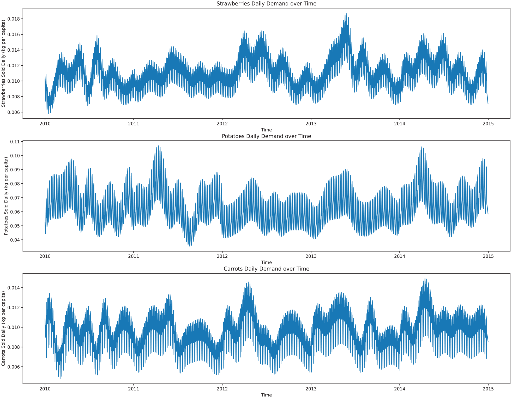
Daily demand functions per customer derived via interpolation from historical statistics.

5.3. Discussion

As an investigation of RQ1, we introduced a methodology combining interpolation and optimization to generate daily demand data from monthly and yearly historical statistics.

Correctness. The optimization solver succeeds in finding solutions where the daily demand summed across the year is effectively equal to the yearly demand total. Insignificant numerical differences can be observed due to optimization thresholds, but this error is certainly less than 1%. Monthly totals can experience more significant levels of error from an expected initialization point, but drastic differences are limited due to the selection of the basis points. Furthermore, as data are limited to 1 year of monthly sales, noise is applied to monthly values regardless, so this error can be considered as a form of extra noise or variation.

Seasonality. Clear seasonality patterns can be observed in Figure 4. Strawberries provide the clearest example with significant increases in sales volumes summer periods (mid-year). Peak volume periods shift slightly from year to year, which can be expected in reality.

Diversity. There is a clear variation in demand patterns across the years. However, in some cases, the diversity may be exaggerated. Looking at the example of strawberries, there is a month in 2010 which experiences a massive decrease in strawberry demand. Given that we have data limited to data on a monthly granularity only for 1 year, it is difficult to assess the realism of such a drop. Such drastic changes could be prevented by decreasing the amount of added noise. The cubic interpolation technique also likely produces a bias in demand curves. For the purposes of training, larger diversity in demands can lead to more robust decision-making systems, albeit likely less optimized.

RQ1: Synthetic daily demand functions which provide correctness, seasonality, and diversity can be generated by careful selection of initial basis points and optimization to decrease error compared to an interpolated view between the basis points and expected aggregate totals. Our methodology enables the creation of high-quality examples even when store-specific data are unavailable.

6. Experimental evaluation

This section provides experimental results and discussion regarding the RL and simulation approach. We investigate the following two research questions independently of RQ1 as they directly relate to the targeted goal of food waste reduction in food retail.

RQ2: How effective are various RL algorithms in managing the ordering of fresh grocery products?

2.1: What is the effect on food waste?

2.2: What is the effect on profit?

2.3: How stable is training for each algorithm?

2.4: How do different reward functions affect performance and stability?

RQ3: What is the runtime of the different components in our simulation framework?

3.1: How long does it take to simulate 1 year of a food retail store operations?

3.2: How much computation time is taken by each RL agent during 100k training steps?

3.3: How much computation time is taken by each RL agent during inference?

6.1. Experimental setup

The entities described in Section 4.1 are initialized with the following parameters:

The wholesaler sells strawberries, potatoes, and carrots at their respective average historical weekly farm prices.⁵² It takes 2 days to ship an order from the wholesaler to a store.

The customer group is a population of 10,000 whose purchases reflect the demand determined in Section 5.

The store sets the price of products according to the historical weekly average retail prices in Atlanta, USA.⁵² See Figure 5.

Figure 5.

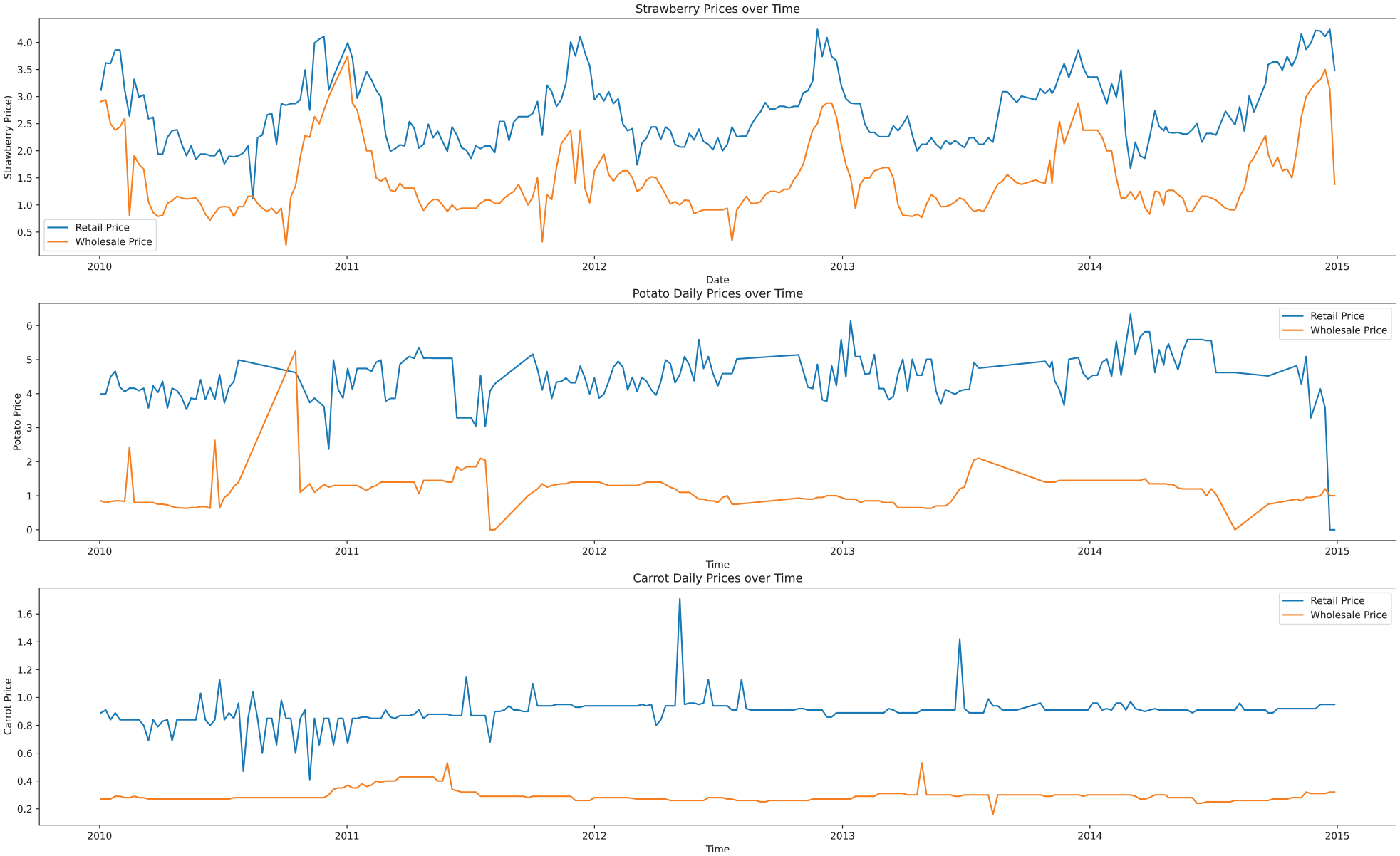
Historical wholesale (orange) and retail (blue) prices for strawberries, potatoes, and carrots.

Product expiration dates are assumed to be the following:

Strawberries have a time to expiration of $N (8, 1)$ .

Potatoes have a time to expiration of $N (75, 5)$ .

Carrots have a time to expiration of $N (28, 3)$ .

These assumptions were derived from the mean time to expiration for each product type and expected intervals.

While some existing works (e.g., Broekmeulen and Van Donselaar³²) model customer behavior wherein the customer always purchases the freshest product, we chose not to model their behavior in this way. Many retailers have processes to push FEFO (“first expiring, first out”). Oftentimes retailers use strategies such as organizing visible inventory so oldest products remain on top or hiding fresher inventory. Some consumers also undoubtedly apply their own strategies to seek fresher products. As such, we model a uniform distribution of consumer selection likelihood from available items. All items of a particular product group get the same pricing. The simulator architecture allows for these different modeling formulations and we plan to address these in a future work where we focus on further refining product ordering and pricing strategies.

Learning. Agents are allowed to learn from simulations of days between 1 January 2010 and 1 January 2012. Up to 100k steps can be used for training with normal demand variation from Gaussian noise. Agents are trained across a range of hyperparameters and initializations. Best performing (on the training set) variants are evaluated on unseen data.

Evaluating and comparing agents. Each agent is evaluated across 1000 simulation runs taking place from 1 January 2012 to 1 January 2015. Simulation runs omit hypothetical catastrophic unexpected events (e.g., pandemic). We provide two baselines. BASE1 implements and evaluates an agent which orders the sum of the product purchases from the past week (yields industry typical near 40% food waste). BASE2 implements the baseline in the work by Broekmeulen and Van Donselaar³² and Tekin and Gürler Berk³³ which monitors a dynamic reorder level, $s_{t} = SS + \sum_{i = t + 1}^{t + L} E [D_{i}]$ . $SS$ is the safety stock, $L$ is the lead time, and $E [D_{i}]$ is the expected demand. If the inventory $I_{t}$ is less than $s_{t}$ , BASE2 orders $s_{t} - I_{t}$ items. We set $SS$ to the expected demand across the next week. In addition, we also provide an optimal profit reference line, OPT, found by satisfying exactly full daily demand without food waste. We compare three RL algorithms: PPO, SAC, and DQN.

Actions. Each agent seeks to learn a policy to optimize an order quantity action for a given state observation. As such, each action value provided by an agent is translated into an order quantity. DQN provides discrete action values, SAC yields continuous action values, and we test PPO in both discrete (PPO-D) and continuous settings (PPO-C). Discrete algorithms designate between 10 preset action values increasing by constant quantities, such as 0, 100, 200, and so on. The maximum order quantity actions are set to be approximately 2 weeks of maximum daily demand. This decreases the range of possible orders to ascertain a reasonable action space. Different discretizations could make a difference, with more potential actions to choose requiring more learning, and fewer resulting in too large of jumps between possible quantities to near optimal. We re-emphasize, in this particular experimentation setup, that the RL agents do not set the prices as actions (see above parameters).

Observations. All algorithm results presented in Section 6 had access to the following observations, normalized to fall within the range of $[0, 1]$ :

The day of the week using one-hot encoding.

The current inventory of each product as a number of items. The algorithms do not have visibility into the age or freshness of individual items.

The purchase quantity of each product over past week.

A forecast which falls within $20 %$ of the actual demand is provided to the agent. We create this synthetic forecast by sampling noise randomly from the uniform distribution and adding it to the demand.

Rewards Each algorithm is trained with both the following reward functions:

REW1 is defined as $sales - ordered$ , where $sales$ is the monetary value of products purchased and $ordered$ is the expenditure on ordering products. For clarity, the agent has some observations derived from the true state and performs an action. The $ordered$ value is the money spent on the order action, and $sales$ is the revenue of sales from this action until the next one.

REW2 is defined as $sales - ordered - PEN (inv < thresh)$ which adds an additional penalty term if the inventory drops below a threshold. In our case, we set the threshold to the daily average demand over the past week. The penalty increases linearly as the inventory drops below this point. This is accomplished by multiplying the penalty value by $1 - \frac{inv}{thresh}$ . This multiplication forces a minimal penalty when inventory is just below the threshold and grows linearly to full penalty as the inventory gets to 0. For $inv > = thresh$ , there is no penalty.

REW1 serves as an optimization for profit, our key optimization target. $Ordered$ encompasses both what is sold (perhaps in subsequent timesteps) and waste. REW2 adds the penalty term to smooth the steep reward cliff of pure profit. Maximizing profit requires minimizing food waste. The profit (and reward) slope drops sharply as waste becomes less than 0. The reward also drops for values greater than 0, albeit less steeply as wholesale prices are lower than retail prices. REW2 attempts to provide a more consistent and less spiky reward signal.

Time dilation. RL environments (such as OpenAI gym⁵³ or gymnasium⁴⁴) typically expect that all actions are performed sequentially and that a reward from the previous action is given along with the current observation for which the next action is taken. In an attempt to mitigate the known negative effect of delays on RL techniques,⁵⁴ we introduce a “time warp” during learning (not present during testing). As delivery of products takes 2 days after an order action, we log/freeze the observations on the day an order action would be taken, but continue simulating until the order would arrive. At this point we return the reward calculated to this time, have the agent provide an action for previously observed state, and create an “instantaneous delivery.” The agent’s observability remains exactly the same, the products arrive at the exact same time, but the reward is better temporally correlated with the relevant action which should help estimating value functions.

6.2. RQ2: effectiveness of RL algorithms

Experiment results are presented in Figure 6 and summarized in Table 1.

Figure 6.

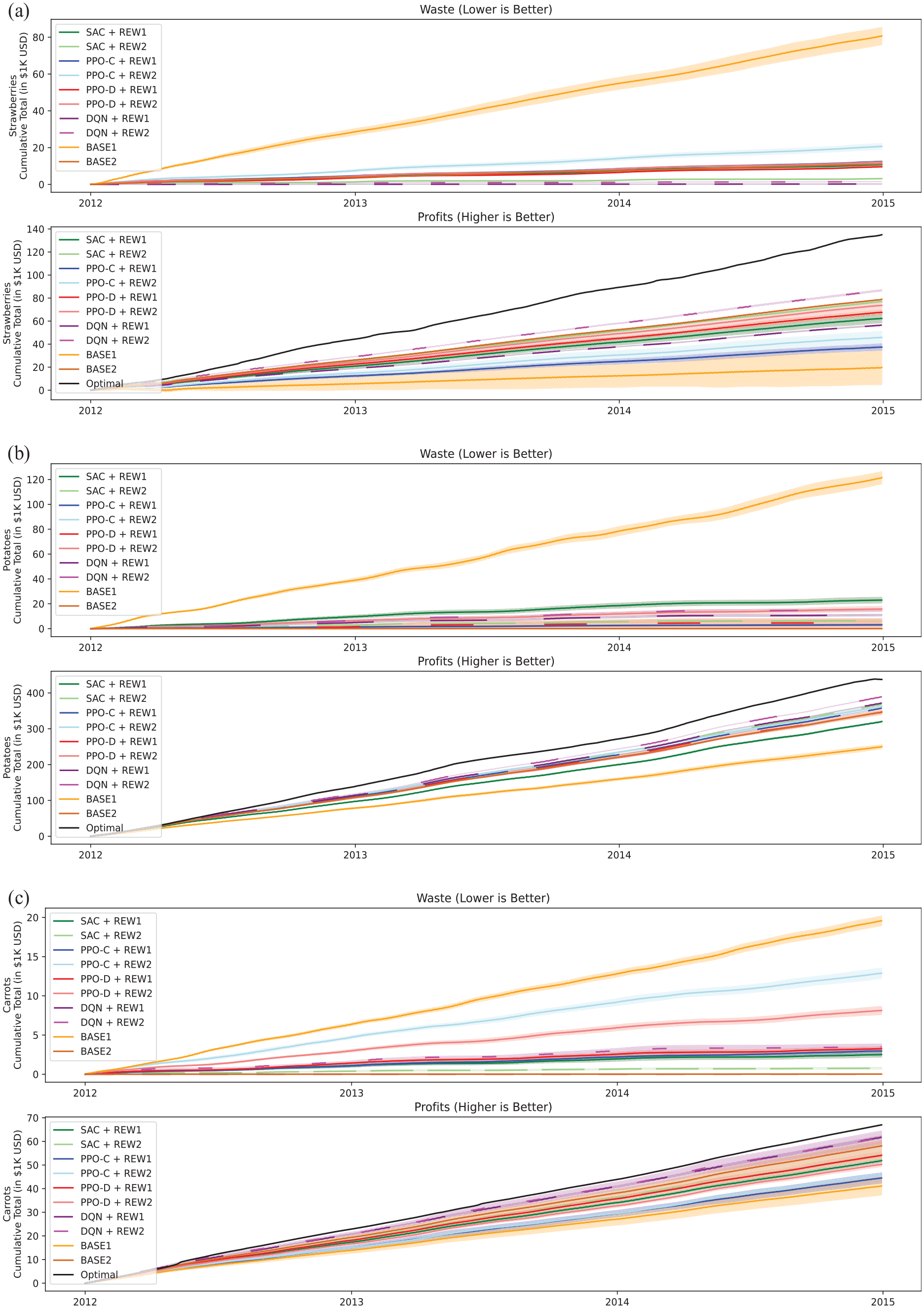
Cumulative waste (top) and cumulative profit (bottom) for (a) strawberries, (b) potatoes, and (c) carrots in USD across 1000 simulations for BASE1, BASE2, SAC, PPO-C, PPO-D, DQN: mean and std. deviation.

Table 1.

Cumulative waste and profits for each RL algorithm and product compared to two baselines.

	Strawberries			Potatoes			Carrots
	Waste (%)	Waste (US$)	Profits (US$)	Waste (%)	Waste (US$)	Profits (US$)	Waste (%)	Waste (US$)	Profits (US$)
OPT	-	-	135k	-	-	437.6k	-	-	67.0k
BASE1	40.3	80.7k	19.7k	39.5	121.5k	250.2k	39.5	19.6k	41.1k
BASE2	7.8	11.1k	78.9k	0.0	0.0k	346.9k	0.1	0.1k	58.1k
PPO-C
REW1	15.4	12.3k	37.3k	1.7	3.0k	357.8k	11.0	3.0k	44.5k
REW2	18.6	20.6k	45.7k	0.0	0.0k	362.5k	30.7	12.9k	46k
PPO-D
REW1	7.5	9.6k	67.5k	2.3	4.5k	346.2k	9.5	3.2k	54.1k
REW2	8.5	12.1k	73.5k	7.5	15.8k	347.1k	20.4	7.4k	48.5k
SAC
REW1	8.9	10.7k	62.2k	11.1	23.0k	320.2k	7.8	2.5k	51.9k
REW2	2.3	3.1k	77k	3.2	6.3k	368.4k	2.4	0.7k	54.2k
DQN
REW1	0.3	0.3k	56.3k	5.3	10.9k	372.0k	0.3	0.1k	61.8k
REW2	1.1	1.5k	86.6k	6.8	15.0k	389.6k	9.1	3.5k	61.5k

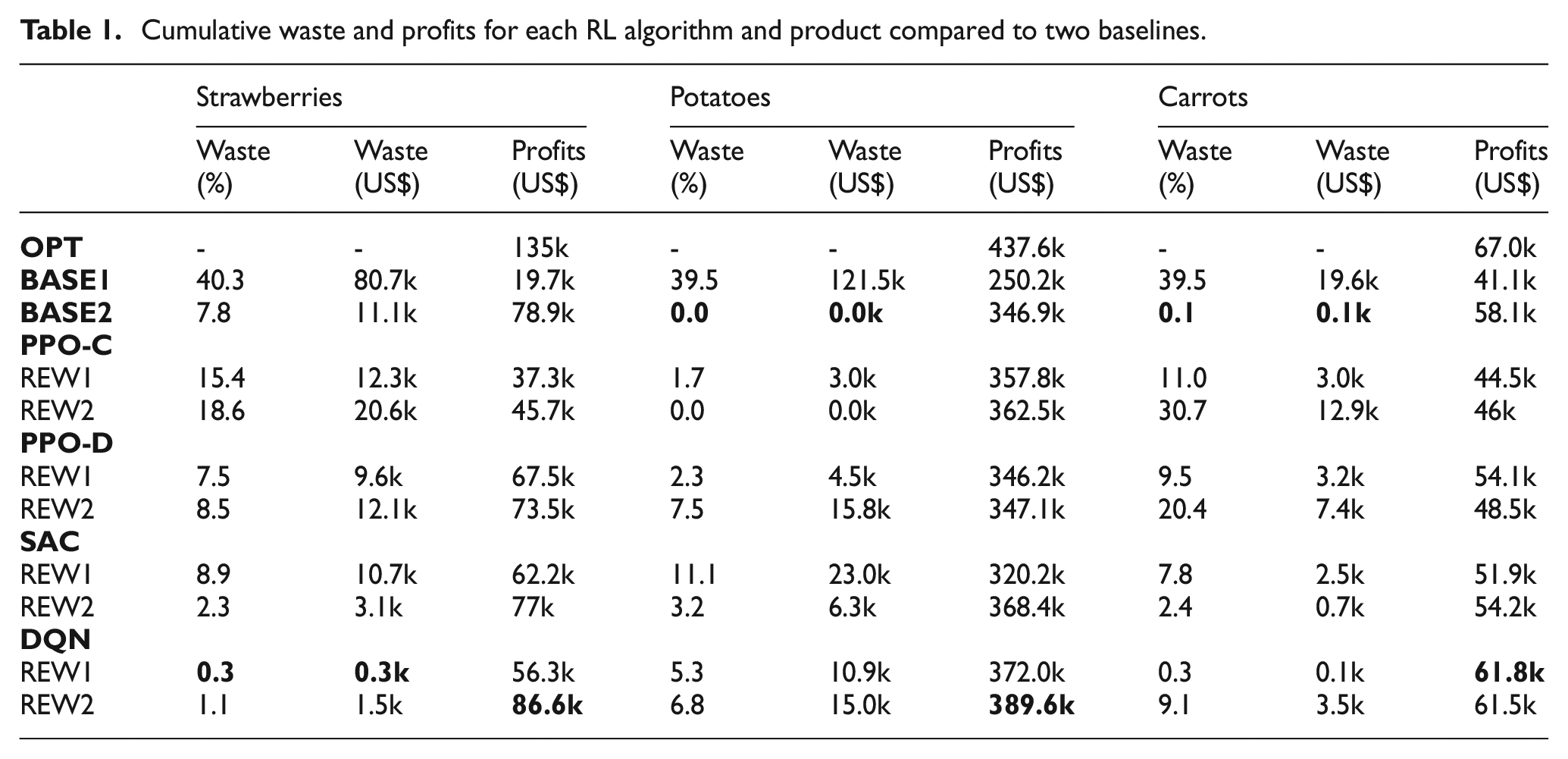
6.2.1. Experimental results

In RQ2, we investigate how effective various RL algorithms are at managing fresh grocery product ordering. Table 1 highlights that each algorithm can reduce food waste and increase profit for each product as compared to BASE1. However, the degree of waste reduction and profit optimization is not consistent across products and algorithms. Moreover, not every RL algorithm yielded better results than BASE2.

Food waste. Each product exhibits unique demand, seasonal, and pricing characteristics. BASE1 produced food waste totals in the vicinity of the industry standard 40%. Each RL algorithm reduced food waste as compared to the BASE1, with some producing negligible food waste (PPO-C + REW2 for potatoes) and others wasting up to 30.7% (PPO-C + REW2 on carrots). On average, RL algorithms reduced food waste by 89.1%, 92.0%, 78.6% and saved retailers US$71.9k, US$111.8k, and US$15.4k in sunk cost for strawberries, potatoes, and carrots, respectively, as compared to BASE1. BASE2 produced nearly no waste for potatoes (0.0%+) and carrots (0.1%) and yielded 7.8% food waste or US$11.1k as sunk cost.

As seen in the example of PPO-C + REW2, there is limited consistency in the algorithm performance. Optimization of the profit-based reward functions sometimes resulted in low food waste totals and at other times larger amounts. No single algorithm or reward scheme produced lowest food waste totals for each products. It can be expected that REW2 should lead to policies that result in more food waste. This is not a guarantee, with 4/12 times the same algorithm trained with REW1 produced more food waste than the same algorithm trained with REW2. Given that strawberries have very short times to expiration, it was expected that high food waste quantities are inevitable. However, all RL algorithms except for PPO-C produced sub-10% food waste regardless if trained using REW1 or REW2. A potential explanation is that due to smaller profit margins and high likelihood of spoilage, optimizing the rewards resulted in the algorithms finding local optima wherein demand is not fully satisfied.

Profit. All algorithms and reward formulations are capable of improving profitability across all three items. DQN achieved the highest profits across all strawberries, potatoes, and carrots, and improved on BASE1 profits by 340%, 56%, and 50%, respectively. It also resulted in 9.8%, 12.3%, and 6.3% better profits than BASE2. Furthermore, it achieved 64.1%, 89%, and 91.8% optimality with respect to highest theoretically achievable profit. This supports findings in related work where DQN achieves high performance in similar problem spaces. The largest performance gap with respect to absolute optimal performance (which also allows for daily ordering) is found in strawberries. This is likely the result of a combination of strawberries having the lowest retail to wholesale price ratios, shortest times to expiration, and high variability in demand. REW2 tended to produce higher profits, despite higher food waste. For example, DQN trained with REW1 resulted in fewer profits than PPO-D trained with REW1 in the case of strawberries. In addition, PPO-D resulted in greater profits than PPO-C on both strawberries and carrots, but lower profits in the case of potatoes.

Stability. Algorithms trained with REW2 typically provide better training stability than those trained with REW1. In the case of REW1, the algorithms were rewarded for reducing the amount of waste until the moment of no waste. However, REW1 can induce a reward “cliff” where decreases in order sizes can result in fewer profits due to not covering full demand while increases in order sizes can result in increased waste. This can make it difficult to appropriately adjust the policy. REW2’s more gradual reward function formulation helps prevent this case by providing a smoother gradient from the threshold to this cliff moment. SAC with REW1 was observed to be the least stable algorithm in training. In fact, some poor training cycles could lead it to extremely low profits and no-food waste and no signs of being able to recover. Of course, adjustment of training parameters such as learning rate could improve stability. It was found that checkpoints, which achieve good performance on the training period, exhibit good performance on the test period, regardless of whether prior training instability was encountered or not.

Learning curves. Not all algorithms improved at the same rate per epoch. Given the prior discussion on instability, in this paragraph, we ignore the periods where the rewards became instable and drop heavily prior to recovering. In this analysis, DQN learned quickly and achieved reasonably high rewards in few epochs and then grew its mean rewards very slowly over time (ignoring some periods of instability which would drop rewards until the algorithm recovered). PPO-C and SAC tended to suffer from poor rewards for a substantial number of epochs compared to DQN but with a significant growth in reward per epoch until the reward saturated and very minimal improvement was seen over time. PPO-D was faster to achieve reasonable rewards, albeit not as quickly as DQN. This general pattern across algorithms could be seen across a multitude of hyperparamaters, including learning rates, batch sizes, discount factors, and algorithm-specific hyperparameters. These of course could change the degree of the pattern seen.

RQ2: RL algorithms can be highly effective for managing the ordering of fresh grocery products. On average, PPO, SAC, and DQN reduced food waste by 78%–92% and increased profit by 50%–340% wrt. BASE1. Likewise, DQN yielded better profits than BASE2 across all products by 6.3%–12.3%. Training may suffer from poor stability but does not prevent the applicability of the approach.

6.2.2. Discussion

Demonstration. Our experimental results showcase that simulation-trained RL can simultaneously significantly reduce food waste and improve business profitability. Undoubtedly, our results could still be improved via better algorithms, rewards, and observation configurations, but this presents a clear proof-of-concept and validity in the approach.

Impact. This work confirms that AI techniques, such as RL, can provide high business impact for food retailers. The demonstrated food waste reductions and increases in profit provide clear environmental and business impact.

Limitations. For a real business scenario, additional factors may need to be incorporated into reward structures. E.g., to maintain customer satisfaction, there should always be products available (i.e., beauty stock) even though it may result in additional food waste. This is a likely reason why food waste metrics more closely align with the results of BASE1 than BASE2 which is pulled from inventory management literature. These experiments were trained on and tested using generated synthetic data. Testing these algorithms on real daily sales data would provide increased confidence in the results.

We plan to more thoroughly investigate RL for improving business profitability in future work, now that we have a validated modular simulation framework. In this investigation, we plan to explore the scalability of an RL approach to thousands of products and to provide the RL algorithms the opportunity to adjust prices.

6.3. RQ3: simulation runtime

6.3.1. Experimental results

In RQ3, we investigate the time spent on simulation computation versus training to profile various algorithms and identify potential performance bottlenecks. An Apple M1 chip is used in our measurements.

Computation. Table 2 presents the computation time each algorithm uses to complete 100k training or inference (non-learning) steps. Times are reported as the mean of 10 non-parallelized runs wherein the algorithms are set to the default Stablebaselines3 hyperparameters. Our simple non-RL BASE1 algorithm requires very little computation, so it can serve as a gauge for simulation time; it takes less than 0.1 s to simulate a year. The results suggest that even neural network computations for inference take longer than for a simulation step to be completed, implying maximum theoretical speedup achievable by increasing simulation speed is around 2x if using the same algorithms and implementations. While there is limited variation in inference times between algorithms, their training times differ substantially. SAC takes the longest amount of time to train and PPO-D the shortest. Comparing BASE1’s inference time to the training times, we can see that simulation accounts for 2.7%–15.5% of training time depending on the algorithm, with the majority of computation dedicated to neural networks.

Table 2.

Training and inference times (in seconds) normalized for 100k steps for each algorithm.

	Train	Inference
BASE1	-	22
BASE2	-	27
PPO-C	220	48
PPO-D	142	48
SAC	813	51
DQN	194	47

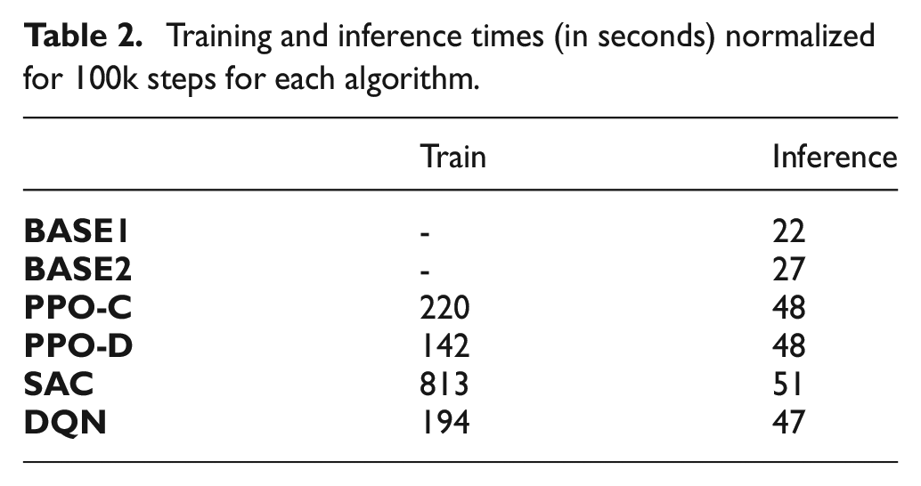
We also measure BASE1’s inference computation time to evaluate multiprocessing-enabled speedup. Using eight threads with a Python implementation without just-in-time compilation, 100k steps can be completed in approximately 3.3 s. This is a 6–7x speedup. We omit multiprocessing results for the RL algorithms as their implementations did not provide parallelization.

RQ3: The simulation environment is efficient as it allows to simulate an entire year within less than 0.1 s. Most computation occurs within the RL agent logic in both training (84%–97%) and inference (53%–57%) where a non-training decision is made using an already learned policy.

6.3.2. Discussion

Demonstration. Our demonstrative case demonstrates that the food retail simulation framework properly handles events and can be used to train and test RL agents or other decision-making systems. Interfaces provide proper access for agents to control product prices and orders. Furthermore, food waste, product deliveries, and purchases are systematically tracked and logged. Each entity is functional; wholesalers, retailers, and customers all interact as expected and customer groups can select between available products. While the demonstrative case used synthetic demand, our framework is highly customizable and configurable which makes future transitions to real daily sales data easy.

Impact. This simulator can serve as both a testbed for research and a real food retail operations tool in the future. It can be deployed as a software service with a public interface, which would enable a smooth transition toward integrated solutions to be used by individual food retailers.

Limitations. RL agents improve with experience. Fast simulation times therefore enable quicker learning as the agent can process more experience per second of computation. While simulation takes less computation time than the RL agents, it could still be optimized to speed up learning. Presently, the simulation environment is written in python without any specialized optimizations, such as just-in-time compilation. This significantly limits the possible computation speeds achievable by the simulator architecture. To improve computation time beyond just-in-time compilation, one can rewrite parts of the simulator in C ++ and connect them to python interfaces via python wrappers. From previous experience, this can result in significant simulation speedups.

Currently, the simulation is limited to daily time steps. In the future, transitioning toward a DEVS framework could allow for finer-detailed modeling.

6.4. Threats to validity

Construct validity. In our demonstrative case, we limit threats to construct validity by initializing simulations from aggregated statistical data. While, this may not be perfectly representative for simulating a realistic food retail location, the data are derived from real sources with seeming consistency (see Section 5.1). We maintain historical average pricing and extract data from average historical demand, which we believe mitigates the threat of simulating a completely unrealistic food retail location.

Internal validity. To avoid threats to internal validity, we use implementations from a trusted library (stablebaselines3) and present the results on the backdrop of a simple baseline. Final evaluation results are the average of 1000 simulation runs to prevent lucky performance. Many metrics and simulation intermediary results are logged to prevent likelihood of inconsistent results.

External validity. The results exhibited in this paper are not guaranteed to be reproduced if the same methodology is adopted by a real food retailer. We seek to mitigate threats to external validity by leveraging data sources based on average statistics to try and create an “average” food retail store.

7. Conclusion

This paper presents a novel food retail simulation framework designed for developing and testing RL solutions for reducing food waste and improving business profitability. As relying on historical data alone is usually insufficient for training such solutions, this work provides a simulation training and test bed, where RL algorithms can be exposed to many food retail scenarios. The DES environment is highly customizable with definable wholesalers, stores, and customers which interact on a daily basis. Any entity can be independently controlled via RL agents or other control algorithms. Logs and statistics of purchases, deliveries, and food waste are all recorded to enable data analysis. We provide a simulation + RL demonstrative case consisting of strawberries, potatoes, and carrots derived from yearly and monthly statistics via a method combining interpolation and optimization. Results for PPO, SAC, and DQN demonstrate that RL methods can significantly improve on a baseline strategy which mimics industry typical 40% food waste. These algorithms reduced food waste by 78%–92% on average with 50%–340% increases in profit. Best algorithms likewise improved on profits from a second well-known baseline from literature by 11.1% on average. Such optimizations would provide true environmental and business impact.

In future work, we will extend our simulation to follow a DEVS framework to improve operations realism and prepare it for working with real food retailers. Furthermore, we will conduct a rigorous investigation across a larger number of algorithms, problem formulations, and algorithms (including multi-armed bandits with delay⁵⁴) to control pricing and order quantities. The goal is to evaluate the ability of such technology to be fully applied in practice and its ability to scale to thousands of retail items.

Footnotes

Funding

This research was partially supported by the Natural Sciences and Engineering Research Council of Canada Idea-to-Innovation (grant no. NSERC I2IPJ 576543-22), a TechAccelR (grant no. #243794) grant and the Invention To Impact (I-to-I) program of McGill Engine. The third author was also supported by the Wallenberg AI, Autonomous Systems and Software Program (WASP) funded by the Knut and Alice Wallenberg Foundation.

ORCID iD

Sebastian Pilarski

Author biographies

Sebastian Pilarski is a PhD from the Department of Electrical and Computer Engineering at McGill University. His research interests include software engineering, machine learning, reinforcement learning, and their applications to systems engineering. He has been working as a Research Scientist at Google’s X, the Moonshot Factory.

Aman Sidhu is a Masters (Thesis) student in the Department of Electrical and Computer Engineering at McGill University and a member of the MILA-affiliated ISMART Lab. His research interests include machine learning, reinforcement learning, robotics, and their applications.

Dániel Varró is a WASP professor at Linköping University and an adjunct professor at McGill University. He is a co-author of more than 190 scientific papers with 7 Distinguished Paper Awards, and 3 Most Influential Paper Awards. He serves on the editorial board of Software and Systems Modeling journal, and served as a program co-chair of MODELS 2021, SLE 2016, ICMT 2014, and FASE 2013 conferences. He is a co-founder of the VIATRA open-source model query and transformation framework, and IncQuery Labs, a technology-intensive company.

References

Feeding America. Fighting food waste and hunger with food rescue. Chicago, IL: Feeding America, 2024.

Silver

Hubert

Schrittwieser

, et al. A general reinforcement learning algorithm that masters chess, shogi, and go through self-play. Science 2018; 362: 1140–1144.

Teller

Holweg

Reiner

, et al. Retail store operations and food waste. J Clean Prod 2018; 185: 981–997.

Baydar . Agent-based modeling and simulation of store performance for personalized pricing. In: Proceedings of the 2003 winter simulation conference, New Orleans, LA, 7–10 December 2003, pp. 1759–1764. New York: IEEE.

Pilarski

Sidhu

Varró

. A simulation environment for reducing food waste via reinforcement learning. In: 2023 annual modeling and simulation conference (ANNSIM), Hamilton, ON, Canada, 23–26 May 2023, pp. 332–344. New York: IEEE.

Zeigler

Kim

Praehofer

Theory of modeling and simulation. Cambridge, MA: Academic Press, 2000.

Sutton

Barto

AG.

Reinforcement learning: an introduction. Cambridge: MIT Press, 2020.

Haarnoja

Zhou

Abbeel

, et al. Soft actor-critic: off-policy maximum entropy deep reinforcement learning with a stochastic actor. In: Int Conf Mach Learn 2018; 80: 1861–1870.

Raffin

Hill

Gleave

, et al. Stable-baselines3: reliable reinforcement learning implementations. J Mach Learn Res 2021; 22: 1–8.

10.

Schulman

Wolski

Dhariwal

, et al. Proximal policy optimization algorithms. arXiv [preprint], 2017. DOI: 10.48550/arXiv.1707.06347.

11.

Schulman

Levine

Abbeel

, et al. Trust region policy optimization. Int Conf Mach Learn 2015; 37: 1889–1897.

12.

Mnih

Kavukcuoglu

Silver

, et al. Playing atari with deep reinforcement learning. arXiv [preprint], 2013. DOI: 10.48550/arXiv.1312.5602.

13.

Bai

Yin

, et al. Simulation based sales forecasting on retail small stores. In: 2008 winter simulation conference, Miami, FL, 7–10 December 2008, pp. 1711–1716. New York: ACM.

14.

Esmaeili

Naghavi

Ghahghaei

Optimal (R, Q) policy and pricing for two-echelon supply chain with lead time and retailer’s service-level incomplete information. J Ind Eng Int 2018; 14: 43–53.

15.

Jandera

Skovranek

Customer behaviour hidden Markov model. Math 2022; 10: 1230.

16.

Kim

Jun

Baek

, et al. Adaptive inventory control models for supply chain management. J Adv Manuf Technol 2005; 26: 1184–1192.

17.

Giannoccaro

Pontrandolfo

Inventory management in supply chains: a reinforcement learning approach. Int J Prod Econ 2002; 78: 153–161.

18.

Chung

A simulation of the impacts of dynamic price management for perishable foods on retailer performance in the presence of need-driven purchasing consumers. J Oper Res Soc 2014; 65: 1177–1188.

19.

Welling

Noel

Ismail

. Identifying potentials and impacts of lead-time based pricing in semiconductor supply chains with discrete-event simulation. In: 2021 winter simulation conference, Phoenix, AZ, 12–15 December 2021, pp. 1–12. New York: IEEE.

20.

Lau

RSM

Xie

Zhao

. Effects of inventory policy on supply chain performance: a simulation study of critical decision parameters. Comput Ind Eng 2008; 55: 620–633.

21.

Christensen

FMM

Solheim-Bojer

Dukovska-Popovska

, et al. Developing new forecasting accuracy measure considering product’s shelf life: effect on availability and waste. J Clean Prod 2021; 288: 125594.

22.

Rao

TR.

Modelling consumer’s purchase behavior as a stochastic process. East Lansing, MI: Michigan State University Press, 1968.

23.

Aaker

Jones

JM.

Modeling store choice behavior. J Mark Res 1971; 8: 38–42.

24.

Schenk

Löffler

Rauh

Agent-based simulation of consumer behavior in grocery shopping on a regional level. J Bus Res 2007; 60: 894–903.

25.

Smith

Nantes

Hogue

, et al. Forecasting customer behaviour in constrained E-commerce platforms. In: 8th international conference of pattern recognition systems (ICPRS), Madrid, 11–13 July 2017, pp. 1–8. New York: IEEE.

26.

Nahmias

Perishable inventory theory: a review. Oper Res 1982; 30: 680–708.

27.

Raafat

Survey of literature on continuously deteriorating inventory models. J Oper Res Soc 1991; 42: 27–37.

28.

Goyal

Giri

BC.

Recent trends in modeling of deteriorating inventory. Eur J Oper Res 2001; 134: 1–16.

29.

Goto

Lewis

Puterman

ML.

Coffee, tea, or…?: a Markov decision process model for airline meal provisioning. Trans Sci 2004; 38: 107–118.

30.

Chen

Tian

Hang

Optimal ordering and pricing policies in managing perishable products with quality deterioration. Int J Prod Res 2021; 59: 4472–4494.

31.

Jia

Dynamic ordering and pricing for a perishable goods supply chain. Comput Ind Eng 2011; 60: 302–309.

32.

Broekmeulen

Van Donselaar

KH.

A heuristic to manage perishable inventory with batch ordering, positive lead-times, and time-varying demand. Comput Oper Res 2009; 36: 3013–3018.

33.

Tekin

Gürler Berk

ÜE.

Age-based vs. Stock level control policies for a perishable inventory system. Eur J Oper Res 2001; 134: 309–329.

34.

Rolf

Jackson

Müller

, et al. A review on reinforcement learning algorithms and applications in supply chain management. Int J Prod Res 2023; 61: 7151–7179.

35.

Chen

Lin

, et al. Effective management for blockchain-based agri-food supply chains using deep reinforcement learning. IEEE Access 2021; 9: 36008–36018.

36.

Afridi

Nieto-Isaza

Ehm

, et al. A deep reinforcement learning approach for optimal replenishment policy in a vendor managed inventory setting for semiconductors. In: 2020 winter simulation conference (WSC), Orlando, FL, 14–18 December 2020, pp. 1753–1764. New York: IEEE.

37.

Oroojlooyjadid

Nazari

Snyder

, et al. A deep Q-network for the beer game with partial information. Comput Res Repos 2017. [arXiv preprint], 48. https://arxiv.org/abs/1708.05924.

38.

Chaharsooghi

Heydari

Zegordi

SH.

A reinforcement learning model for supply chain ordering management: an application to the beer game. Decis Support Syst. 2008;45(4): 949–959.

39.

Gijsbrechts

Boute

Zhang

, et al. Can deep reinforcement learning improve inventory management? Performance on dual sourcing, lost sales and multi-echelon problems. SSRN Electron J. Epub ahead of print 3 January 2019. DOI: 10.2139/ssrn.3302881.

40.

David

Syriani

DEVS model construction as a reinforcement learning problem. In: 2022 annual modeling and simulation conference (ANNSIM), San Diego, CA, 18–20 July 2022, pp. 30–41. New York: IEEE.

41.

Kara

Dogan

Reinforcement learning approaches for specifying ordering policies of perishable inventory systems. Expert Syst Appl 2018; 91: 150–158.

42.

Sun

, et al. Inventory cost control model for fresh product retailers based on DQN. In: 2019 IEEE international conference on big data (big data), Los Angeles, CA, 9–12 December 2019, pp. 5321–5325. New York: IEEE.

43.

Jullien

Ariannezhad

Groth

, et al. A simulation environment and reinforcement learning method for waste reduction. Trans Mach Learn Res 2023. [arXiv preprint], 20. https://openreview.net/forum?id=KSvr8A62MD.

44.

Towers

Terry

Kwiatkowski

, et al. Gymnasium: A standard interface for reinforcement learning environments 2023. arXiv preprint, 6. https://www.researchgate.net/publication/382526464_Gymnasium_A_Standard_Interface_for_Reinforcement_Learning_Environments

45.

USDA Foreign Agricultural Service. Consumption of fresh potatoes in Canada 2009–2019, http://bit.ly/3FpQK2F (2022 accessed 20 December 2022).

46.

Spain Ministry of Agriculture, Food and Environment. Spain: monthly consumption of potatoes2020, http://bit.ly/3TiBWZG (2022 accessed 20 December 2022).

47.

US Department of Agriculture. U.S. fresh strawberries consumption per capita from 2000 to 2020, http://bit.ly/3YHTcZ7 (2022 accessed 20 December 2022).

48.

Spain Ministry of Agriculture, Food and Environment. Spain: monthly fresh fruit consumption 2020, http://bit.ly/3Lo3B9r (2022 accessed 20 December 2022).

49.

US Department of Agriculture; Economic Research Service. Per capita consumption of fresh carrots in the United States from 2000 to 2022 (in pounds), http://bit.ly/479R1mj (2023 accessed 14 November 2023).

50.

Ministry of Agriculture, Food and Environment. Volume of fresh vegetables consumed in Spain from January 2020 to December 2020, https://bit.ly/47whjij (2023 accessed 14 November 2023).

51.

Google Maps. Real Canadian superstore, http://bit.ly/3jhYJa7 (2022 accessed 28 December 2022).

52.

Western Growers. Produce price index, http://www.producepriceindex.com/ (2022 accessed 10 December 2022).

53.

Brockman

Cheung

Pettersson

, et al. OpenAI Gym. 2016. arXiv preprint, 4. https://arxiv.org/abs/1606.01540.

54.