Defining hybrid hierarchical models in π H Y F LOW

Abstract

This paper presents πHyFlow, a modular approach to the process interaction worldview (PI). Traditionally, PI supports a set of interacting processes without enabling modular and hierarchical model definition. πHyFlow basic models define a dynamic set of processes while also enabling a modular interface for supporting model composition. πHyFlow allows an exact representation of continuous signals based on the concepts of dense outputs, and generalized sampling. πHyFlow ability to support accurate models of hybrid systems is presented through a DC-DC converter (DCC) based on a resistor–capacitor (RC) electrical circuit. The DCC output voltage can be modeled by a first-order differential equation that is solved using an exponential time differencing (ETD) integrator. The DCC network model uses a digital on-off controller and an ETD. Simulation results are generated by πHyFlow⁺⁺, a C++ implementation of the formalism.

1. Introduction

The process interaction worldview (PI) provides a simple and expressive framework for modeling complex systems by enabling entities life-cycles to be represented in a single script. In contrast, other approaches, like the event scanning worldview, ¹ scatter entities life-cycles among events, making it more difficult to model complex systems. Traditionally, PI was developed without support for modular models, since all processes coordinate throughout the access to a global shared state.^2,3 Although this approach can support the representation of simple systems, it does not provide the modular and hierarchical constructs required to enable the description of complex systems as a composition of (sub-)systems.

In previous work, we have developed the Hybrid Flow System Specification (HyFlow) formalism to represent hierarchical and modular hybrid systems. ⁴ HyFlow uses generalized sampling and dense outputs as first-order constructs for defining continuous systems. ⁵ HyFlow base models are limited to represent a single event, requiring multiple events to be represented by a network model. This constraint imposes an additional complexity for models that have a simpler representation based on shared memory coordination like, e.g., Petri nets. Given a system where several servers share a common queue, a modular formalism like HyFlow will require a complex synchronization to move customers from the queue to an idle server. On the contrary, a PI model of this system is simpler and more expressive. ⁶ There seems to be a gap between modular modeling formalisms that promote modularity and PI that enables simpler models but lacks the ability to represent complex systems.

πHyFlow ⁷ is an extension of the original HyFlow formalism aimed to support PI while keeping modularity and the ability to modify model topology at runtime. πHyFlow defines a modular base model that hosts a dynamic set of processes. While process intra-communication is made through a shared state, the communication between models is achieved by modular messages. The modeler gains the ability to choose whether a system will be represented by a network of models, or by a set of interacting processes, and use the most suitable approach.

We illustrate πHyFlow ability to represent hybrid systems by modeling a resistor–capacitor (RC) electrical circuit, and a simplified DC-DC step-down converter (DCC). The DCC circuit is used to transform a DC voltage into a lower value for a range of loads. RC and DCC circuits are represented ordinary differential equations (ODEs) whose exact solutions are computed by an Exponential Time Differenting (ETD) integrator. For the DCC circuit, an “on-off” digital controller is used to keep the output voltage within the desired output range.

The paper is organized as follows. Section 2 describes the πHyFlow formalism base and network models. This section also presents the models of rectangular and trigonometric signal generators. Section 3 presents, the RC electrical circuit and the Exponential Time Differencing (ETD) integrator. This section presents also RC implementation in the πHyFlow⁺⁺ modeling & simulation environment. Section 4 presents the DCC model. Section 5 compares πHyFlow with other M&S approaches. A discussion of πHyFlow advantages and limitations, and future work are presented in Section 6. Conclusion is presented in Section 7.

2. The πHyFlow formalism

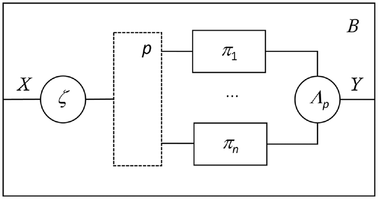
A πHyFlow base model defines a modular entity that encloses a set of processes $\{{\pi }_1,...,{\pi }_n\}$ communicating through a shared p-state $p$ , as represented in Figure 1. Each process keeps its own (private) p-state, and it can perform read/write operations on the shared p-state. Processes have suspend/resume semantics but are non-preemptive making them implementable by coroutines, avoiding the synchronization problems associated with (preemptive) threads. ⁸

Figure 1.

πHyFlow base model structure.

Base models communicate through modular input $\left(X\right)$ and output $\left(Y\right)$ interfaces. A process represents a sequence of actions where each action requires an amount of time $t\ge 0$ to be executed. Processes are coordinated by the base model that acts as a scheduler. When scheduled, the base model chooses a process that is enabled to execute and resumes it. After execution, the process suspends itself and gives the control back to the base model that selects the next process to run. A process becomes enabled when a given time interval has elapsed, or when the current guard condition is fulfilled.

Processes do not have an input, since after their creation, they are suspended at some point on their flows waiting for being re-activated. Process communication with the external entities can only thus be achieved, indirectly, through the shared p-state $p$ , that can be modified by all processes and by the model input function $\zeta$ . Processes, however, have a modular output interface. Base model output is computed by function $\mathrm{\Lambda }=\{{\mathrm{\Lambda }}_p\}$ that uses the outputs from all processes. Since πHyFlow base models have a modular interface, they can be composed to form networks. Formalism is described in the next sections. πHyFlow semantics is provided in Barros. ⁹

2.1. πHyFlow base model

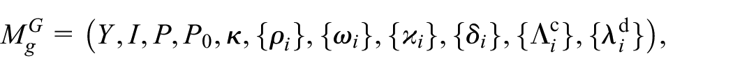
In the original HyFlow formalism, a base model can only schedule one event. πHyFlow removes this constraint by enabling a base model to run several processes, each one with the ability to schedule its own event. Moreover, since processes share a common state, their synchronization becomes easier to achieve when compared with the corresponding HyFlow network model. A πHyFlow base model associated with name $B$ is defined by:

$$M_B=(X,Y,P,P_0,\zeta ,\Pi ,\pi ,\sigma ,\{{\mathrm{\Lambda }}_p\})$$

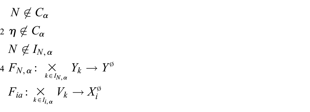
where $X=X^{\mathrm{c}}\times X^{\mathrm{d}}$ is the set of input flow values, with $X^{\mathrm{c}}$ is the set of continuous input flow values, $X^{\mathrm{d}}$ is the set of discrete input flow values, $Y=Y^{\mathrm{c}}\times Y^{\mathrm{d}}$ is the set of output flow values, with $Y^{\mathrm{c}}$ is the set of continuous output flow values, $Y^{\mathrm{d}}$ is the set of discrete output flow values, $P$ is the set of partial shared states (p-states), $P_0$ is the set of (valid) initial p-states, $\zeta :P\times X^{\mathrm{ø}}\to P$ is the input function, with $X^{\mathrm{ø}}=X^{\mathrm{c}}\times (X^{\mathrm{d}}+\mathrm{ø})$ , $\Pi$ is a set of processes, $\pi :P\to \mathcal{P}(\Pi )$ is the current-processes function, where $\mathcal{P}$ is the power set, $\sigma :\mathcal{P}(\Pi )\to {\mathcal{P}}^{*}$ is the ranking function, where ${\mathcal{P}}^{*}$ is the set of all sequences based on set $P$ , constrained to $\sigma (A)=(a_1,\dots ,a_n)\Rightarrow \{a_1,\dots ,a_n\}==A\wedge |\sigma (A)|==|A|$ , for all $p\in P:$ ${\mathrm{\Lambda }}_p:\underset{i\in A}{\times }{Y}_i^{\mathrm{ø}}\to Y^{\mathrm{ø}}$ is the output function associated with p-state $p$ , with $A=\sigma (\pi (p))$ , and $Y^{\mathrm{ø}}=Y^{\mathrm{c}}\times (Y^{\mathrm{d}}+\mathrm{ø})$ .

The base model receives and produces both continuous and discrete flows (events) through the modular interfaces $X$ and $Y$ . The input function $\zeta$ is responsible for updating the current p-state when the model receives a value either by sampling or event communication. The set of processes is dynamic, being the current set defined by function π. Given that processes can access the shared p-state only one can be active at any time. The ranking function $\sigma$ decides process resume order. The output function $\mathrm{\Lambda }=\{{\mathrm{\Lambda }}_p\}$ maps the outputs of all processes into the output associated with the base model. A formal description of πHyFlow processes is provided in the next section.

2.2. πHyFlow process model

As mentioned before, a process represents a sequence of actions where each action requires an amount of time $t\ge 0$ to be executed. Processes are coordinated by the base model that acts as a scheduler. When in control, the base model chooses a process that is enabled to execute and resumes it. After execution, the process suspends itself and gives the control back to the base model that selects the next process to run. A process becomes enabled when a given time interval has elapsed, or when the current guard condition is fulfilled. Given a base model $B$ with a set of processes ${\Pi }_B$ , the model of a process $\varpi \in {\Pi }_B$ is defined by:

$$M_{\varpi }^B=(Y,I,P,P_0,\kappa ,\{{\rho }_i\},\{{\omega }_i\},\{{\mathrm{\varkappa }}_i\},\{{\delta }_i\},\{{\mathrm{\Lambda }}_i^{\mathrm{c}}\},\{{\lambda }_i^{\mathrm{d}}\})$$

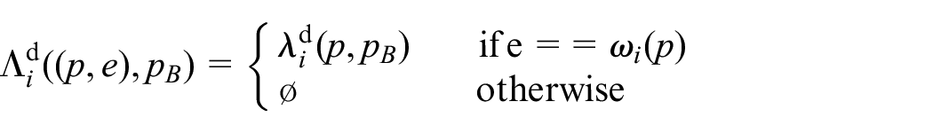
where $Y$ is the set of output flow values, $Y^{\mathrm{c}}$ is the set of continuous output flows, $Y^{\mathrm{d}}$ is the set of discrete output flows, $I$ is the set of indexes, $P$ is the set of p-states, $P_0$ is the set of (valid) initial p-states, $\kappa :P\to I$ is the index function, for all $i\in I:$ ${\rho }_i:P\to {\mathbb{H}}_0^{+\infty }$ is the time-to-input function, ${\omega }_i:P\to {\mathbb{H}}_0^{+\infty }$ is the time-to-output function, ${\mathrm{\varkappa }}_i:P\times P_B\to \{\mathrm{T},\perp \}$ is the condition function, ${\delta }_i:S\times P_B\to P\times P_B$ is the transition function, ${\mathrm{\Lambda }}_i^{\mathrm{c}}:S\times P_B\to Y^{\mathrm{c}}$ is the continuous output function, ${\lambda }_i^{\mathrm{d}}:P\times P_B\to Y^{\mathrm{d}}$ is the partial discrete output function, ${\mathrm{\Lambda }}_i^{\mathrm{d}}:S\times P_B\to Y^{\mathrm{d}}\cup \{\varnothing \}$ is the discrete output function defined by:

$${\mathrm{\Lambda }}_i^{\mathrm{d}}((p,e),p_B)=\{\begin{array}{c}{\lambda }_i^{\mathrm{d}}(p,p_B)\mathrm{if}\mathrm{e}=={\omega }_i(p)\hfill \\ \multicolumn{1}{c}{\mathrm{ø}\mathrm{otherwise}}\end{array}$$

with $S=\{(p,e)|p\in P,0\le e\le {\nu }_{\kappa (p)}(p)\}$ , the state set, and ${\nu }_i(p)=min\{{\rho }_i(p),{\omega }_i(p)\},i=\kappa (p)$ , is the time-to-transition function.

For time specification, πHyFlow uses the set of hyper-real numbers $\mathbb{H}$ , that enables causality to be expressed, by assuming that a transition occurring at time $t$ , changes process p-state at time $t+\epsilon$ , where $\epsilon \in \mathbb{H}$ is an infinitesimal. ⁴ Time functions $\rho$ and $\omega$ are constrained to the positive hyper-real values ${\mathbb{H}}_0^{+\infty }$ .

A process defines only its output $Y$ , while the input is inferred from base model p-state. A process defines its own p-state $P$ , for reducing inter process dependency. A process dynamic behavior is ruled by six structured/segmented functions, being the segments currently active determined by the index function $\kappa$ . The active segments associated with p-state $p\in P$ are $({\rho }_i,{\omega }_i,{\mathrm{\varkappa }}_i,{\delta }_i,{\mathrm{\Lambda }}_i^{\mathrm{c}},{\lambda }_i^{\mathrm{d}}){|}_{i=\kappa (p)}$ .

The time-to-input-function $\{{\rho }_i\}$ specifies the interval for sampling (reading) a value. Since each process specifies its own reading interval, sampling is made asynchronously, and it can be made independently by any process. The concept of generalized sampling refers here to the capability of supporting asynchronous and time-varying sampling. The time-to-input-function establishes sampling as a first-order operator, on par with the traditional concept of event. The time-to-output-function $\{{\omega }_i\}$ specifies the interval to produce a discrete flow. The condition/guard function $\{{\mathrm{\varkappa }}_i\}$ , checks whether the process has conditions to run given base model and process current p-states. Functions $\{{\rho }_i\}$ and $\{{\omega }_i\}$ specify a time interval for process re-activation, while $\{{\mathrm{\varkappa }}_i\}$ checks if the process can be re-activated at the current time. Function $\{{\delta }_i\}$ specifies process and base model p-states after process re-activation. Function $\{{\mathrm{\Lambda }}_i^{\mathrm{c}}\}$ specifies the process continuous output flow, and $\{{\mathrm{\Lambda }}_i^{\mathrm{d}}\}$ specifies the process discrete output flow. The former can be non-null at every time instant, while the latter can only be non-null at a finite number of time instants during a finite time interval. $\{{\mathrm{\Lambda }}_i^{\mathrm{c}}\}$ can provide an exact description for an arbitrary continuous signal based on a discrete formalism. This feature is used in section to describe the continuous output flow of the ETD integrator.

2.3. Trigonometric signal generator

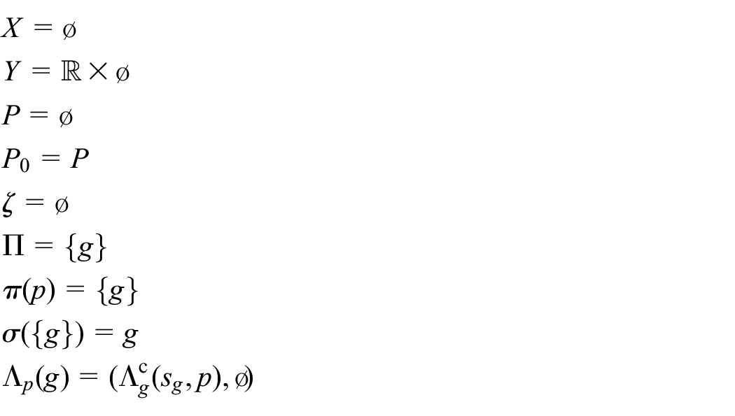
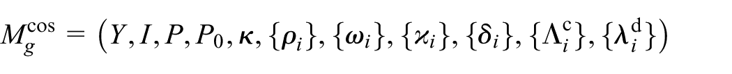
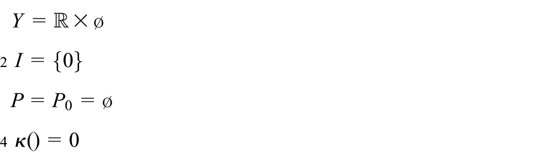
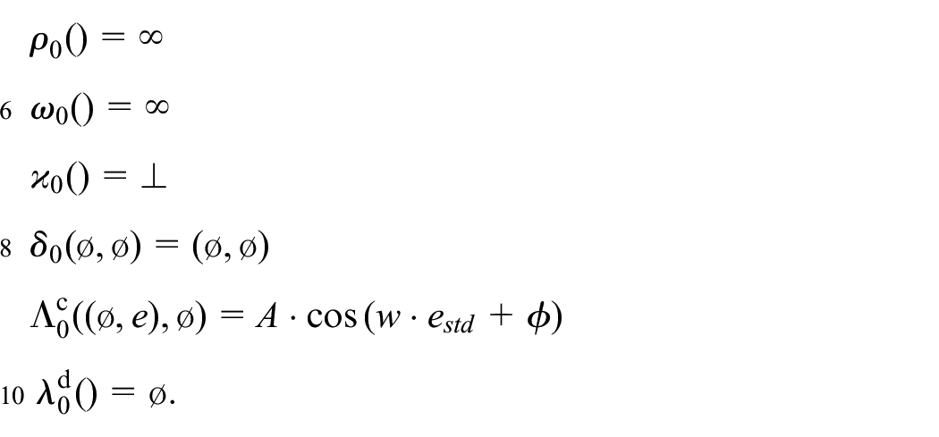
As an example of a πHyFlow base model, we describe a continuous trigonometric signal generator model that produces the output $A\cos (\mathrm{wt}+\varphi )$ . πThe HyFlow base model associated with a generator named “cos” is defined by:

$$M_{\cos }=(X,Y,P,P_0,\zeta ,\Pi ,\pi ,\sigma ,\{{\mathrm{\Lambda }}_p)\}$$

where

$$\begin{array}{c}X=\mathrm{ø}\hfill \\ Y=\mathbb{R}\times \mathrm{ø}\hfill \\ P=\mathrm{ø}\hfill \\ P_0=P\hfill \\ \zeta =\mathrm{ø}\hfill \\ \Pi =\{g\}\hfill \\ \pi (p)=\{g\}\hfill \\ \sigma (\{g\})=g\hfill \\ {\mathrm{\Lambda }}_p(g)=({\mathrm{\Lambda }}_g^{\mathrm{c}}(s_g,p),\mathrm{ø})\hfill \end{array}$$

To simplify the notation symbol $\mathrm{ø}$ is overloaded and it can represent an empty value, an empty set, an empty sequence, or a null function, depending on the context. The model of process $g$ is defined by:

$$M_g^{\cos }=(Y,I,P,P_0,\kappa ,\{{\rho }_i\},\{{\omega }_i\},\{{\mathrm{\varkappa }}_i\},\{{\delta }_i\},\{{\mathrm{\Lambda }}_i^{\mathrm{c}}\},\{{\lambda }_i^{\mathrm{d}}\})$$

where

$$\begin{array}{c}Y=\mathbb{R}\times \mathrm{ø}\\ 2I=\{0\}\\ P=P_0=\mathrm{ø}\\ 4\kappa ()=0\end{array}$$

$$\begin{array}{c}{\rho }_0()=\infty \\ 6{\omega }_0()=\infty \\ {\mathrm{\varkappa }}_0()=\perp \\ 8{\delta }_0(\mathrm{ø},\mathrm{ø})=(\mathrm{ø},\mathrm{ø})\\ {\mathrm{\Lambda }}_0^{\mathrm{c}}((\mathrm{ø},e),\mathrm{ø})=A·\cos (w·e_{\mathrm{std}}+\varphi )\\ 10{\lambda }_0^{\mathrm{d}}()=\mathrm{ø}.\end{array}$$

The generator produces (line 9) the continuous signal $A·\cos (w·e_{\mathrm{std}}+\varphi )$ for the some constants $A,w$ , and $\varphi$ . The standard part of hyper-real $e$ is noted by $e_{\mathrm{std}}$ . The signals are exact, and it can be obtained through sampling at any point in time. We note that this model can be generalized to describe any continuous trajectory.

2.4. Rectangular-wave signal generator

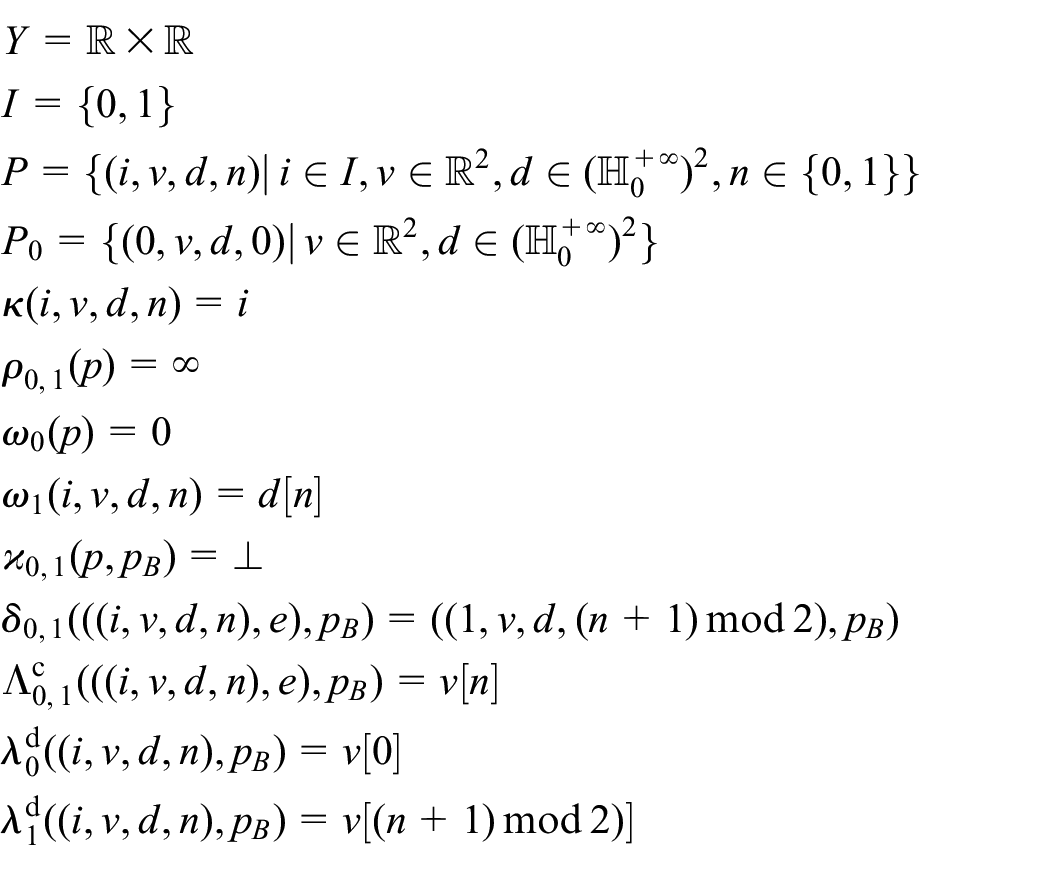
As an additional example of a πHyFlow base model, we describe a piecewise constant signal generator model. The generator produces a periodic piecewise constant signal with amplitude $v_0$ and duration $d_0$ , followed by a constant signal with amplitude $v_1$ and duration $d_1$ . While the continuous flow output is piecewise constant, the discrete flow output is used to signal the discontinuities. The generator defines a process $g$ that sets base model dynamic behavior. The πHyFlow base model associated with a generator named $G$ is defined by:

$$M_G=(X,Y,P,P_0,\zeta ,\Pi ,\pi ,\sigma ,\{{\mathrm{\Lambda }}_p\})$$

where

$$\begin{array}{c}X=\mathrm{ø}\hfill \\ Y=\mathbb{R}\times \mathbb{R}\hfill \\ P=\mathrm{ø}\hfill \\ P_0=P\hfill \\ \zeta =\mathrm{ø}\hfill \\ \Pi =\{g\}\hfill \\ \pi (p)=\{g\}\hfill \\ \sigma (\{g\})=g\hfill \\ {\mathrm{\Lambda }}_p(g)=({\mathrm{\Lambda }}_g^{\mathrm{c}}(s_g,p),{\mathrm{\Lambda }}_g^{\mathrm{d}}(s_g,p))\hfill \end{array}$$

The model of process $g$ is defined by:

$$M_g^G=(Y,I,P,P_0,\kappa ,\{{\rho }_i\},\{{\omega }_i\},\{{\mathrm{\varkappa }}_i\},\{{\delta }_i\},\{{\mathrm{\Lambda }}_i^{\mathrm{c}}\},\{{\lambda }_i^{\mathrm{d}}\}),$$

where

$$\begin{array}{c}Y=\mathbb{R}\times \mathbb{R}\hfill \\ I=\{0,1\}\hfill \\ P=\{(i,v,d,n)|i\in I,v\in {\mathbb{R}}^2,d\in ({\mathbb{H}}_0^{+\infty }{)}^2,n\in \{0,1\}\}\hfill \\ P_0=\{(0,v,d,0)|v\in {\mathbb{R}}^2,d\in ({\mathbb{H}}_0^{+\infty }{)}^2\}\hfill \\ \kappa (i,v,d,n)=i\hfill \\ {\rho }_{0,1}(p)=\infty \hfill \\ {\omega }_0(p)=0\hfill \\ {\omega }_1(i,v,d,n)=d[n]\hfill \\ {\mathrm{\varkappa }}_{0,1}(p,p_B)=\perp \hfill \\ {\delta }_{0,1}(((i,v,d,n),e),p_B)=((1,v,d,(n+1)\mathrm{mod}2),p_B)\hfill \\ {\mathrm{\Lambda }}_{0,1}^{\mathrm{c}}(((i,v,d,n),e),p_B)=v[n]\hfill \\ {\lambda }_0^{\mathrm{d}}((i,v,d,n),p_B)=v[0]\hfill \\ {\lambda }_1^{\mathrm{d}}((i,v,d,n),p_B)=v[(n+1)\mathrm{mod}2)]\hfill \end{array}$$

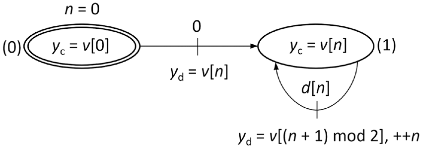
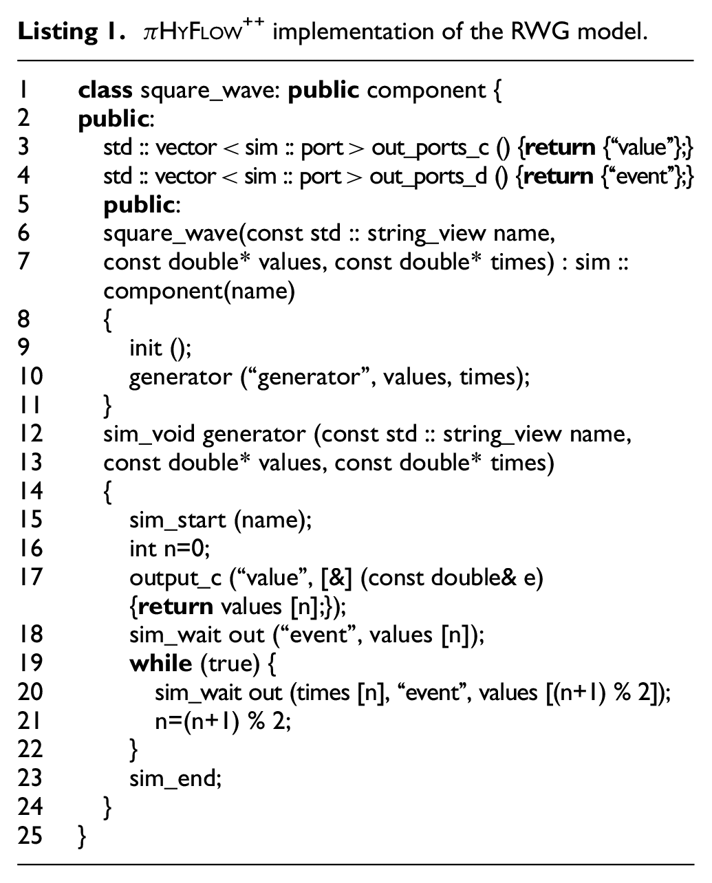
Generator state diagram is depicted in Figure 2. The generator starts at index (0), and the current piecewise constant segment $n$ is set 0. At index 0, the model switches immediately (zero time delay) to index 1, while it sends the discrete flow $y_{\mathrm{d}}=v[0]$ . The model loops in index (1). After the delay $d[n]$ , it produces the discrete flow $y_{\mathrm{d}}$ and updates $n$ . The continuous output flow is always present and is given by $y_{\mathrm{c}}$ . The implementation using coroutines is described in Listing 1 that provides a simpler syntax.

Figure 2.

RWG state diagram.

Listing 1.

πHyFlow⁺⁺ implementation of the RWG model.

1 2 3 4 5 6 7 8 9 10 11 12 13 14 15 16 17 18 19 20 21 22 23 24 25

class square_wave: public component { public:  std :: vector<sim :: port>out_ports_c () {return {“value”};}  std :: vector<sim :: port>out_ports_d () {return {“event”};}  public:  square_wave(const std :: string_view name,  const double* values, const double* times) : sim :: component(name)  {   init ();   generator (“generator”, values, times);  }  sim_void generator (const std :: string_view name,  const double* values, const double* times)  {   sim_start (name);   int n=0;   output_c (“value”, [&] (const double& e) {return values [n];});   sim_wait out (“event”, values [n]);   while (true) {    sim_wait out (times [n], “event”, values [(n+1) % 2]);    n=(n+1) % 2;   }   sim_end;  } }

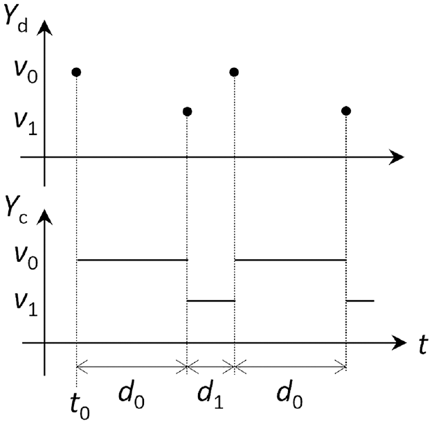
Generator output trajectory is depicted in Figure 3. The generator starts at time $t_0$ and it issues the discrete flow $v_0$ . The continuous flow $v_0$ becomes available for sampling during the interval $d_0$ . At time $t_0+d_0$ , the generator issues the discrete flow $d_1$ . During this interval, the constant value $v_1$ is produced as the generator continuous output flow. This cycle repeats making the signal periodic. In general, a πHyFlow base model can receive and produce continuous and discrete flows. A base model can also define an arbitrary number of processes. The set of processes is dynamic, and processes can be created and destroyed at runtime.

Figure 3.

RWG output trajectory.

2.5. πHyFlow network model

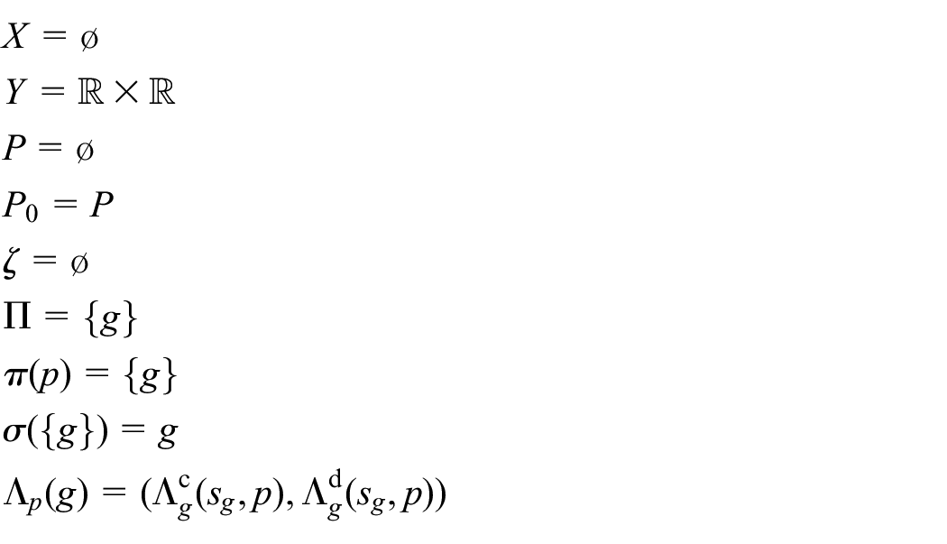
A πHyFlow network is composed by base or other network models. In addition, each network has a special component, named as executive, that is responsible for defining network topology (composition and coupling). A πHyFlow network model associated with name $N$ is defined by:

$$M_N=(X,Y,\eta )$$

where $N$ is the network name, $X=X^{\mathrm{c}}\times X^{\mathrm{d}}$ is the set of network input flows, $Y=Y^{\mathrm{c}}\times Y^{\mathrm{d}}$ is the set of network output flows, and $\eta$ is the name of the network executive.

The executive is a $\pi$ HyFlow base model extended with topology related operators. The executive model is defined by:

$$M_{\eta }=(X,Y,P,P_0,\zeta ,\Pi ,\pi ,\{{\mathrm{\Lambda }}_p\},{\Sigma }^{*},\gamma )$$

where ${\Sigma }^{*}$ is the set of network topologies, and $\gamma :P\to {\Sigma }^{*}$ is the topology function.

The network topology $\gamma (p_{\alpha })\in \Sigma$ , corresponding to the p-state $p_{\alpha }\in P$ , is given by:

$$\gamma (p_{\alpha })=(C_{\alpha },\{I_{i,\alpha }\},I_{\eta ,\alpha },I_{N,\alpha },\{F_{i,\alpha }\},F_{\eta ,\alpha },F_{N,\alpha })$$

where $C_{\alpha }$ is the set of names associated with the executive p-state $p_{\alpha }$ , for all $i\in C_{\alpha }$ : $I_{i,\alpha }$ is the sequence of influencers of $i$ , $F_{i,\alpha }$ is the input function of $i$ , $I_{\eta ,\alpha }$ is the sequence of executive influencers, $I_{N,\alpha }$ is the sequence of network influencers, $F_{\eta ,\alpha }$ is the executive input function, and $F_{N,\alpha }$ is the network output function, for all $i\in C_{\alpha }$ $M_i=(X,Y,P,P_0,\zeta ,\Pi ,\pi ,\sigma ,\{{\mathrm{\Lambda }}_p\})$ , for base models, and $M_i=(X,Y,\eta )$ , for network models.

Functions $\{F_{i,\alpha }\},F_{\eta ,\alpha }$ , and $F_{N,\alpha }$ enable to compose any arbitrary πHyFlow models, since these functions can be used to match arbitrary model interfaces. Variables and functions are subjected to the following constraints for all $p_{\alpha }\in P_{\alpha }$ :

$$\begin{array}{c}N\notin C_{\alpha }\hfill \\ 2\eta \notin C_{\alpha }\hfill \\ N\notin I_{N,\alpha }\hfill \\ 4F_{N,\alpha }:\underset{k\in I_{N,\alpha }}{\times }{Y}_k\to Y^{\mathrm{ø}}\hfill \\ F_{\mathrm{ia}}:\underset{k\in I_{i,\alpha }}{\times }{V}_k\to X_i^{\mathrm{ø}}\hfill \end{array}$$

$$\begin{array}{c}6\mathrm{where}{V}_k=\{\begin{array}{cc}{Y}_k^{\mathrm{ø}}\hfill & \mathrm{if}k\ne N\hfill \\ \multicolumn{1}{c}{X^{\mathrm{ø}}}& \mathrm{if}k=N\hfill \\ F_{N,\alpha }((v_{\mathrm{c},k_1},\mathrm{ø}),(v_{\mathrm{c},k_2},\mathrm{ø}),...)=(y_{\mathrm{c},N},\mathrm{ø})\hfill \\ 8F_{i,\alpha }((v_{\mathrm{c},k_1},\mathrm{ø}),(v_{\mathrm{c},k_2},\mathrm{ø}),...)=(x_{\mathrm{c},i},\mathrm{ø})\hfill \end{array}\hfill \end{array}$$

Constraints 1 and 2 impose that the executive cannot remove neither the network nor itself. Constraint 3 enforces causality (section). Constraints 7 and 8 are a characteristic of discrete systems and impose that a non-null discrete flow cannot be created from a sequence composed exclusively of null discrete flows. Network topology is defined by executive function $\gamma$ that maps executive p-state into network composition and coupling. Coupling information includes, for each model, a set of influencers and an input function. Changes in executive p-state can be mapped into changes in network topology, enabling the definition of dynamic structure models. Since HyFlow models have a continuous output flow, the sampling operation reads atomically all current outputs from the influencers’ models and applies the input function, providing the influenced model with a single input value. This operation provides thus support for interface matching. The network has an output function for mapping the output values of its influencers into the network output $Y$ . Likewise the base HyFlow formalism ⁴ networks and base models are kept during simulation, enabling the co-simulation of πHyFlow models. The next section describes an RC electric circuit as a πHyFlow network model.

3. RC circuit

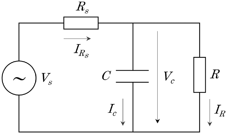
For illustrating the πHyFlow network model defined in the previous section, we consider the RC circuit of Figure 4. The circuit includes capacitor $C$ , resistors $R$ and $R_s$ , and voltage source $V_s$ , requiring the solution of a first-order ODE.

Figure 4.

RC circuit with a time-varying voltage source.

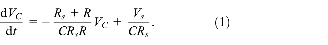
The voltage $V_C$ in the circuit is given by:

$$\frac{\mathrm{d}{V}_C}{\mathrm{d}t}=-\frac{R_s+R}{C{R}_{s}R}{V}_C+\frac{V_s}{C{R}_s}.$$

(1)

We describe next the ETD numerical integrator that is used to solve Equation (1).

3.1. ETD

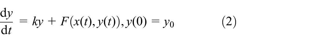
The ETD enables exact solutions for some systems or the possibility of using large stepsizes, when solving stiff ODEs. ¹⁰ ETD considers ODEs in the form of:

$$\frac{\mathrm{d}y}{\mathrm{d}t}=\mathrm{ky}+F(x(t),y(t)),y(0)=y_0$$

(2)

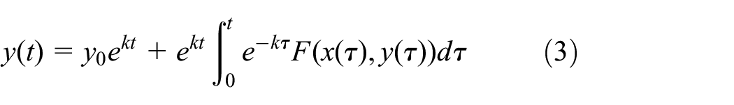
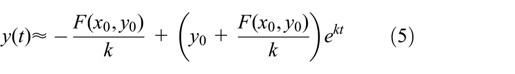
where $k$ is a constant coefficient and $F$ represents the non-linear part. The exact solution for $t\in [0,T]$ is given by: ¹⁰

$$y(t)=y_0{e}^{\mathrm{kt}}+e^{\mathrm{kt}}{\int }_0^t{e}^{-k\tau }F(x(\tau ),y(\tau ))d\tau$$

(3)

Considering the zeroth-order approximation for $F$ :

$$F(x(t),y(t))\approx F(x(0),y(0))$$

(4)

the corresponding approximation for the solution $y(t),t\in [0,T]$ is given by:

$$y(t)\approx -\frac{F(x_0,y_0)}{k}+(y_0+\frac{F(x_0,y_0)}{k})e^{\mathrm{kt}}$$

(5)

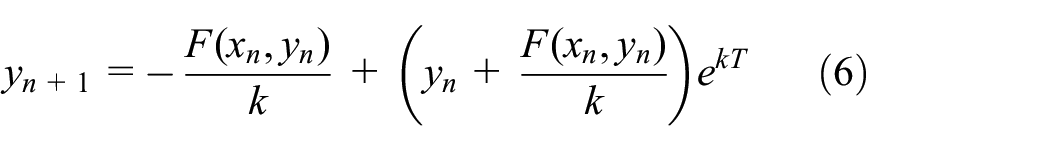
yielding the numerical integrator with a fixed sampling interval $T$ described by:

$$y_{n+1}=-\frac{F(x_n,y_n)}{k}+(y_n+\frac{F(x_n,y_n)}{k})e^{\mathrm{kT}}$$

(6)

Equation (6) can be used for numerical integration. Equation (5) provides the dense output between steps. This equation can be computed in a similar manner to the trigonometric generator of section . If we constraint the input signal $F$ to be piecewise constant, Equation (5) becomes exact, and the ETD can be driven by input discontinuities, obviating the use of sampling (stepsize =  $\infty$ ).

3.2. RC network model

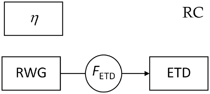
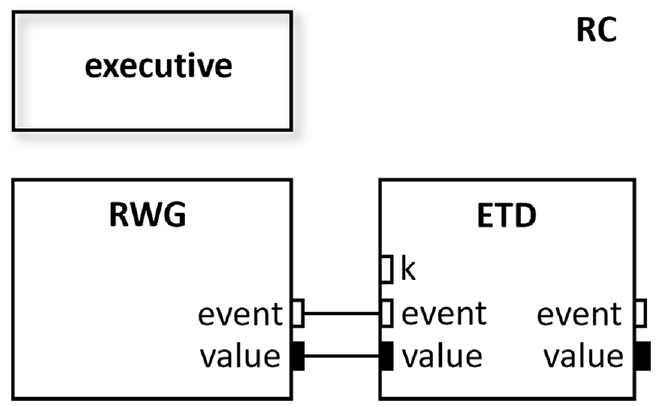
The RC circuit of Figure 4 can be represented by the πHyFlow network model shown in Figure 5. Besides the executive $\eta$ that defines the (static) network topology, the model has a rectangular-wave signal generator (RWG) component and an ETD component. The πHyFlow network model for the circuit is defined by $M_{\mathrm{RC}}=(\mathrm{ø},\mathrm{ø},\eta )$ , where the executive model is given by:

$$M_{\eta }=(\mathrm{ø},\mathrm{ø},\mathrm{ø},\mathrm{ø},\mathrm{ø},\mathrm{ø},\mathrm{ø},\mathrm{ø},\{{\Sigma }_0\},\gamma )$$

where ${\Sigma }_0$ is the (static) network topology, $\gamma ()={\Sigma }_0$ , with ${\Sigma }_0=(\{\mathrm{RWG},\mathrm{ETD}\},\{\mathrm{ø},I_{\mathrm{ETD}}\},\mathrm{ø},\mathrm{ø},\{\mathrm{ø},F_{\mathrm{ETD}}\},\mathrm{ø},\mathrm{ø})$ , where $I_{\mathrm{ETD}}=(\mathrm{RWG})$ , and $F_{\mathrm{ETD}}(x_{\mathrm{c}},x_{\mathrm{d}})=(x_{\mathrm{c}},x_{\mathrm{d}})$ .

Figure 5.

πHyFlow network model of the RC circuit.

Model $M_{\mathrm{RWG}}$ is defined in section, and model $M_{\mathrm{ETD}}$ is described in Barros. ⁷ The next section provides simulation results for this model obtained using the πHyFlow⁺⁺ M&S environment.

3.3. RC circuit simulation results

πHyFlow⁺⁺ is an implementation of πHyFlow in MSVC++ 20. πHyFlow⁺⁺ uses C++ support for modules, variants, lambdas, and coroutines. It uses the concept of port to segment continuous and discrete flows. For each input continuous flow port, there is a merge function to enable a port to sample from several components at once. The merge function computes the combination of the several input samples. For each input discrete flow port, πHyFlow⁺⁺ assigns an input buffer that collects all values directed to that port. Each continuous output port is assigned to a process that defines a function parameterized by the elapsed time since process last transition. Listing 1 provides the πHyFlow⁺⁺ implementation of the rectangular-wave model described in section .

The RWG defines the continuous flow output port “value,” and the discrete output flow port “event” (lines 3–4). The continuous flow is defined in line 17. Although for an RWG this value is piecewise constant, the elapsed time “e” enables the definition of arbitrary continuous flow outputs. The process loops within lines 19–22. It holds for a time interval and it sends an event (line 20) corresponding to a new constant continuous output value. The rectangular-wave segment is updated in line 21.

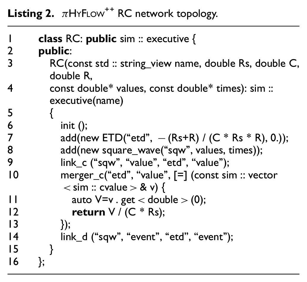
The πHyFlow⁺⁺ RC network is depicted in Figure 6 and defined in Listing 2. The ETD component sets the ODE coefficient (line 7) according to Equation (1). The ETD also has port “k” enabling the coefficient to be modified at runtime.

Figure 6.

RC πHyFlow network representation.

Listing 2.

πHyFlow⁺⁺ RC network topology.

1	class RC: public sim :: executive {
2	public:
3	RC(const std :: string_view name, double Rs, double C, double R,
4	const double* values, const double* times): sim :: executive(name)
5	{
6	init ();
7	add(new ETD(“etd”, −(Rs+R) / (C * Rs * R), 0.));
8	add(new square_wave(“sqw”, values, times));
9	link_c (“sqw”, “value”, “etd”, “value”);
10	merger_c(“etd”, “value”, [=] (const sim :: vector<sim :: cvalue>& v) {
11	auto V=v . get<double>(0);
12	return V / (C * Rs);
13	});
14	link_d (“sqw”, “event”, “etd”, “event”);
15	}
16	};

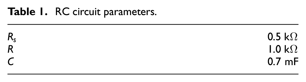
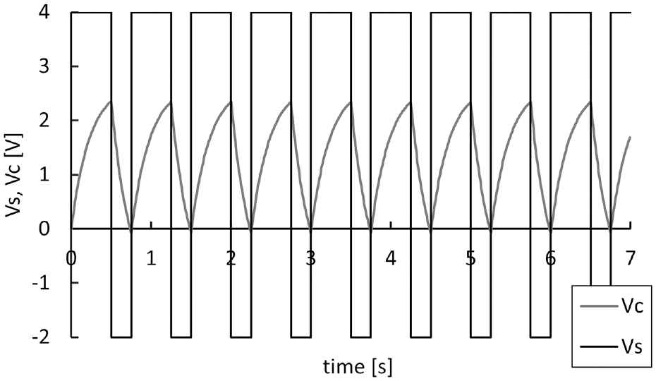
The merge function of the ETD is defined in lines 10–13, and the input value is set according to Equation (1). By default, links between discrete flow ports (line 14) define an identity function. For simulation, we have used the parameters defined in Table 1. The rectangular-wave generator has parameters (4 V, −2 V, 0.5 s, 0.25 s). Figure 7 shows results for a simulation time of 7 s. Given circuit parameters, the ETD integrator yields exact simulation results.

Table 1.

RC circuit parameters.

$R_s$	0.5 $\mathrm{k}\Omega$
$R$	1.0 $\mathrm{k}\Omega$
$C$	0.7 mF

Figure 7.

Voltage source $V_s$ , and capacitor voltage $V_c$ for the RC circuit.

4. DC voltage converter (DCC)

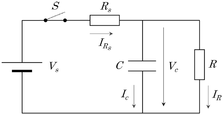
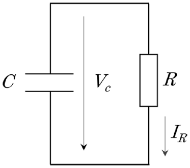
A DC-DC step-down converter (DCC) transforms an input DC voltage $V_s$ into a lower output voltage $V_{\mathrm{ref}}<V_s$ . For simplicity, we consider here a simple first-order DCC based on a resister and a capacitor. Second-order converters based on a combination of capacitors and inductors have also been developed. ¹¹ The DCC is represented in Figure 8, and it is composed by a voltage source $V_s$ in series with a switch $S$ , a resistor $R_S$ , and a capacitor $C$ . The load $R$ is connected to the capacitor terminals. The switch position is set by an on-off digital controller that samples the voltage $V_C$ and compares it with the reference $V_{\mathrm{ref}}$ value. The switch is turned on when $V_C<V_{\mathrm{ref}}$ and off otherwise. When the switch is turned off, the circuit can be described by Figure 9, and the capacitor acts as a voltage source that feeds current $I_R$ through the load $R$ . The switch is operated by a digital controller described in section .

Figure 8.

DCC topology when the switch $S$ is “on.”

Figure 9.

DCC topology when the switch is “off.”

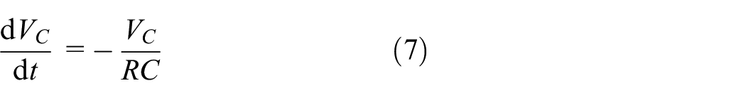
When the switch $S$ is “on,” the voltage $V_C$ is given by Equation (1). When $S$ is “off,” the voltage $V_C$ is given by:

$$\frac{\mathrm{d}{V}_C}{\mathrm{d}t}=-\frac{V_C}{\mathrm{RC}}$$

(7)

Equations (1) and (7) are the first-order ODEs that can be solved without error by the ETD integrator described in section .

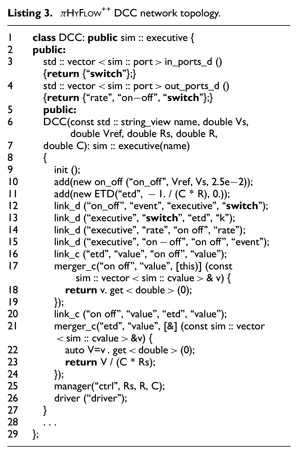
4.1. πHyFlow⁺⁺ DCC implementation

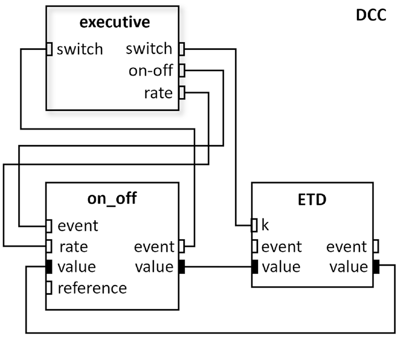
The DCC is modeled by the πHyFlow network model depicted in Figure 10 and defined by πHyFlow⁺⁺ (Listing 3). The network is composed by the executive, the ETD, and the on-off digital controller. As mentioned in section, the executive is responsible to keep network topology (composition and coupling). The executive is also responsible to update ETD coefficient $k$ when the switch changes through the output port “switch.” The executive has also port “on-off” to activate/deactivate the digital controller, and port “rate” to set controller sampling interval. To simplify DCC modeling, the controller acts both as a mechanism to turn the switch on/off, and as a voltage source.

Figure 10.

DC converter network topology.

Listing 3.

πHyFlow⁺⁺ DCC network topology.

1 2	class DCC: public sim :: executive { public:
3 4 5	std :: vector<sim :: port>in_ports_d () {return {“switch”};}  std :: vector<sim :: port>out_ports_d () {return {“rate”, “on−off”, “switch”};}  public:
6	DCC(const std :: string_view name, double Vs, double Vref, double Rs, double R,
7	double C): sim :: executive(name)
8 9	{   init ();
10	add(new on_off (“on_off”, Vref, Vs, 2.5e−2));
11	add(new ETD(“etd”, −1. / (C * R), 0.));
12	link_d (“on_off”, “event”, “executive”, “switch”);
13	link_d (“executive”, “switch”, “etd”, “k”);
14	link_d (“executive”, “rate”, “on off”, “rate”);
15	link_d (“executive”, “on−off”, “on off”, “event”);
16	link_c (“etd”, “value”, “on off”, “value”);
17	merger_c(“on off”, “value”, [this)] (const
18	sim :: vector<sim :: cvalue>& v) {   return v. get<double>(0);
19 20	});   link_c (“on off”, “value”, “etd”, “value”);
21	merger_c(“etd”, “value”, [&] (const sim :: vector<sim :: cvalue>&v) {
22	auto V=v . get<double>(0);
23	return V / (C * Rs);
24 25	});   manager(“ctrl”, Rs, R, C);
26	driver (“driver”);
27 28	}  . . .
29	};

The controller has a sampling rate of $2.5\times {10}^{-2}$  s (line 10). Lines 12–16 and 20 define the links shown in Figure 10. The merger functions associated with controller continuous input flow port “value” is defined in lines 17–19. The ETD samples the controller, and the value is given by Equation (1), being computed in lines 21–25 where the controller output is given by variable “V.”

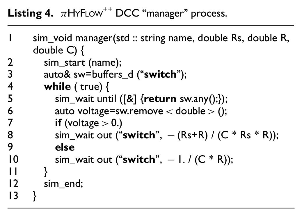
The executive runs processes “manager” (line 25) and“driver” (line 26). Process “manager,” defined in Listing 4, is responsible to update ETD coefficient “k.” When a “switch” discrete flow is received, the “manager” process checks the voltage and sends the new coefficient “k” through the output port “switch.” This value is received at ETD input port “k” as shown in Figure 10.

Listing 4.

πHyFlow⁺⁺ DCC “manager” process.

1 2	sim_void manager(std :: string name, double Rs, double R, double C) {  sim_start (name);
3	auto& sw=buffers_d (“switch”);
4 5 6	while ( true) {   sim_wait until ([&] {return sw.any();});   auto voltage=sw.remove<double>();
7	if (voltage>0.)
8	sim_wait out (“switch”, −(Rs+R) / (C * Rs * R));
9	else
10	sim_wait out (“switch”, −1. / (C * R));
11 12	}  sim_end;
13	}

Line 8 corresponds to Equation (1) defining the circuit of Figure 8, and line 10 corresponds to Equation (7) defining the circuit of Figure 9. Process “driver” is defined in the section and defines the experimental conditions for DCC simulation. Next section provides the implementation of the on-off controller model.

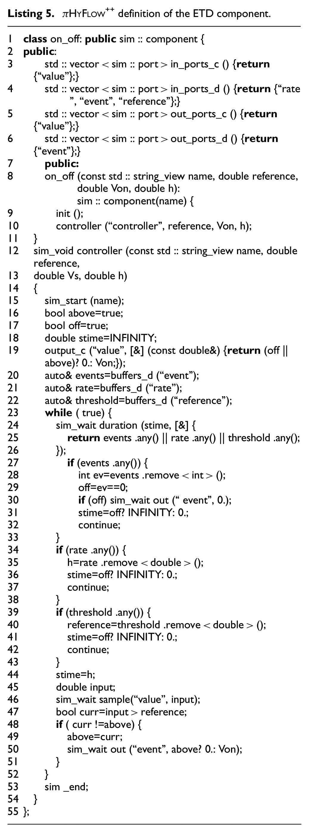
4.2. πHyFlow⁺⁺ on-off digital controller

An off-off digital controller samples its input at some time interval and it produces the output discrete flows $V_{\mathrm{on}}$ and 0, when the input is below or above a reference value, respectively. The sampling interval is commonly fixed, but arbitrary irregular intervals can also be described in πHyFlow⁺⁺. πHyFlow⁺⁺ implementation of the on-off controller model is represented in Listing 5. The component has continuous input port “value” where it samples the input voltage. The reference voltage is set when the component is created. This value can also be modified at runtime through the discrete flow port “reference.” The component has discrete input port “event” to activate/deactivate the controller. Port “rate” sets controller sampling interval.

Listing 5.

πHyFlow⁺⁺ definition of the ETD component.

1	class on_off: public sim :: component {
2	public:
3	std :: vector<sim :: port>in_ports_c () {return {“value”};}
4	std :: vector<sim :: port>in_ports_d () {return {“rate ”, “event”, “reference”};}
5	std :: vector<sim :: port>out_ports_c () {return {“value”};}
6	std :: vector<sim :: port>out_ports_d () {return {“event”};}
7	public:
8	on_off (const std :: string_view name, double reference, double Von, double h): sim :: component(name) {
9	init ();
10	controller (“controller”, reference, Von, h);
11	}
12	sim_void controller (const std :: string_view name, double reference,
13	double Vs, double h)
14	{
15	sim_start (name);
16	bool above=true;
17	bool off=true;
18	double stime=INFINITY;
19	output_c (“value”, [&] (const double&) {return (off || above)? 0.: Von;});
20	auto& events=buffers_d (“event”);
21	auto& rate=buffers_d (“rate”);
22	auto& threshold=buffers_d (“reference”);
23	while ( true) {
24	sim_wait duration (stime, [&] {
25	return events .any() || rate .any() || threshold .any();
26	});
27	if (events .any()) {
28	int ev=events .remove<int>();
29	off=ev==0;
30	if (off) sim_wait out (“ event”, 0.);
31	stime=off? INFINITY: 0.;
32	continue;
33	}
34	if (rate .any()) {
35	h=rate .remove<double>();
36	stime=off? INFINITY: 0.;
37	continue;
38	}
39	if (threshold .any()) {
40	reference=threshold .remove<double>();
41	stime=off? INFINITY: 0.;
42	continue;
43	}
44	stime=h;
45	double input;
46	sim_wait sample(“value”, input);
47	bool curr=input>reference;
48	if ( curr !=above) {
49	above=curr;
50	sim_wait out (“event”, above? 0.: Von);
51	}
52	}
53	sim _end;
54	}
55	};

The controller has a continuous output port “value” with the current output value. Changes in the output value are signaled through discrete output port “event.”

The controller has a fixed sampling interval of “stime” (line 24). This interval can be interrupted when there is an event to: stop the controller, change the sampling rate, or change the reference value (line 25). These events are handled in lines 27–33, 34–38, and 39–43, respectively. Controller continuous output value is defined in line 19. This value is 0 when the controller is deactivated or when the most recent sampled value is above the reference. The input value is sampled in line 46. For simulation efficiency, the on-off discrete flow is only sent if it is different from the previous value (lines 48–51). The controller is initially deactivated (line 17). Next section presents simulation results for the DCC model.

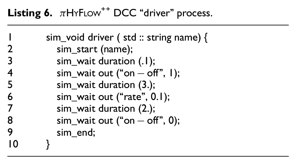
4.3. DCC simulation results

DCC simulation was performed using the process “driver” defined in Listing 6. The controller is initially deactivated, and it has a default sampling interval of 50 ms. The controller is activated at time 0.1 s (lines 3–4). After a duration of 3.0 s, controller sampling interval is set to 100 ms (lines 5 and 6). The controller becomes inactive after 2.0 s (lines 7 and 8).

Listing 6.

πHyFlow⁺⁺ DCC “driver” process.

1	sim_void driver ( std :: string name) {
2	sim_start (name);
3	sim_wait duration (.1);
4	sim_wait out (“on−off”, 1);
5	sim_wait duration (3.);
6	sim_wait out (“rate”, 0.1);
7	sim_wait duration (2.);
8	sim_wait out (“on−off”, 0);
9	sim_end;
10	}

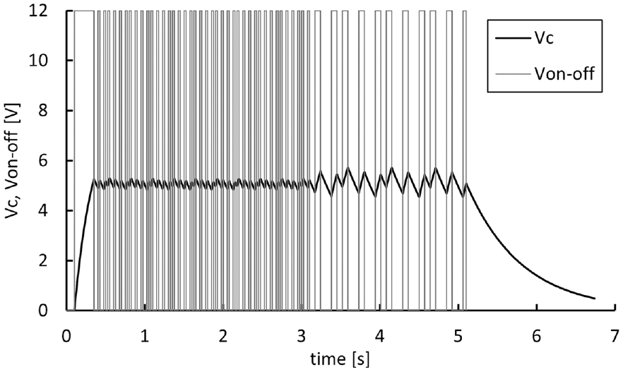
Simulation was performed using circuit parameters described in Table 1, $V_{\mathrm{on}}=V_s=12\mathrm{V}$ , and $V_{\mathrm{ref}}=5\mathrm{V}$ . As mentioned before, when activated, the controller commands the DCC, producing a piecewise constant signal of 0 V, when the voltage $V_C$ is above the reference value $V_{\mathrm{ref}}$ , and 12 V when the voltage is below $V_{\mathrm{ref}}$ . Simulation results for controller output $V_{\mathrm{on}-\mathrm{off}}$ , and capacitor voltage $V_C$ are shown in Figure 11.

Figure 11.

Capacitor voltage $V_C$ and controller output $V_{\mathrm{on}-\mathrm{off}}$ , for $V_{\mathrm{ref}}$  = 6 V.

The controller is turned on at time 0.1 s and the 12 V voltage is applied until time 0.35 s when the output voltage $V_C=5.25985$ V >  $V_{\mathrm{ref}}$ . Voltage $V_C$ oscillates around $V_{\mathrm{ref}}=5\mathrm{V}$ . The amplitude of oscillations increases when the sampling interval is doubled at time 3.1 s. The controller is turned off at time 5.1 s and $V_C$ exponentially decreases after that time. Given that controller output is piecewise constant, the ETD defined by Equation (6) yields an exact solution. The ETD is also very efficient since it is driven entirely by the events that change the ODE parameter $k$ of Equation (6), requiring, for this model, no extra samples that would be required, e.g., by polynomial integrators to ensure a bound in solution error.

4.4. DCC with rectangular-wave voltage reference

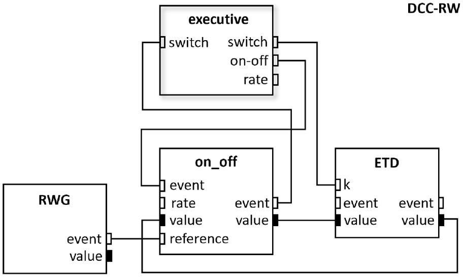
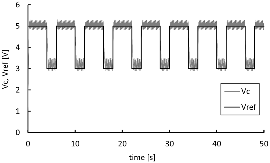
The DCC described before has a constant reference voltage. This value can be modified, as mentioned in section, through on-off controller port “reference.” We can create a DCC with a variable voltage by composing the controller with a rectangular-wave generator. Figure 12 represents the new DCC with rectangular-wave voltage reference (DCC-RW) model, where RWG port “event” is connected to controller port “reference,” forcing the DCC to follow the RWG output value that is used as a time-varying reference. For simulation, we have used the RC circuit parameters of Table 1, and a rectangular wave with parameters (5 V, 3 V, 4 s, 2 s) used as a time-varying reference. Results are shown in Figure 13 for a simulation time of 50 s.

Figure 12.

DCC with a rectangular-wave reference voltage.

Figure 13.

Capacitor voltage $V_C$ and reference voltage $V_{\mathrm{ref}}$ .

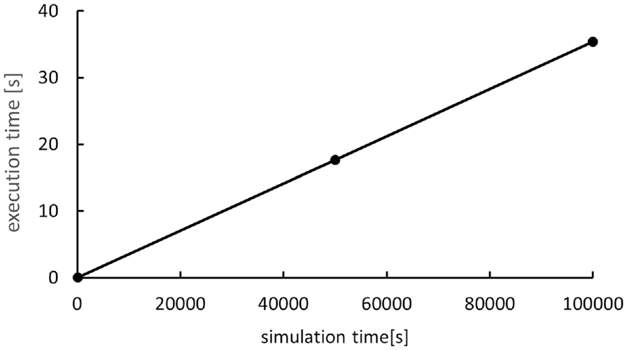
Preliminary performance results are shown in Figure 14 that presents the real simulation time of the DCC-RW circuit for several simulation times. Given the reduced number of processes the simulations can be efficiently performed. However, handling a large number of threads will require optimizations in the event queue, and in process conditional testing as discussed in section.

Figure 14.

DCC-RW execution time × simulation time.

5. Related work

The process interaction worldview (PI) was introduced in GPSS ¹² and SIMULA ² languages, and it enables a representation based on the flow of systems’ entities. Frameworks supporting PI based on C++, ¹³ Python, ¹⁴ and Java ¹⁵ have also been developed, but they do not support modular and hierarchical models. The formal specification of PI was introduced in Zeigler. ³ This work was limited to non-modular models, based on a static set of processes. A general approach to process conditional waiting was proposed in Cota and Sargent. ¹⁶ This work, however, did not add any support to model modularity.

PI makes it easier to model complex systems ⁶ when compared to other worldviews, like the event scheduling. ¹ πHyFlow, an extension of HyFlow formalism, enables the representation of hybrid systems using PI while supporting also modular and hierarchical models.

Traditionally, the representation of continuous/hybrid systems involves the composition of models using a facade modular graphical user interface (GUI), being the set of resulting ODEs flattened for numerical integration. ¹⁷ Although a model can have a modular appearance, its simulation may not be modular. Models are usually translated into a set of ODEs/Differencial Algebraic Equations that are solved with a common type of numerical integrator. The combination of heterogeneous integrators like ETD or geometric solvers is not possible, affecting the fidelity of models. Model flattening poses also problems for supporting changes in model topology.

To the best of our knowledge, generalized sampling was introduced in author work.^5,18 Multirate numerical integrators have also been developed.^19,20,21 These approaches, however, do not provide a modular representation of ODEs. On the contrary, CFSS support for generalized sampling and continuous outputs enables the definition of modular numerical integrators. In addition, CFSS modular integrators not only can sample at different sampling rates but also can have time-varying sampling rates. CFSS enables the seamless composition of different families of numerical integrators. The concept of elapsed time used in CFSS to produce continuous flows was formalized in DEVS. ³

CFSS supports co-simulation since it guarantees modularity of both models and the corresponding simulation. πHyFlow uses CFSS operators to enable an accurate description of continuous signals. The support for multiple clocks was introduced in Esterel ²² and Modelica ²³ languages, but continuous flows are limited to piecewise constant segments. These limitations do not enable the representation of continuous flows required, e.g., to model the ETD integrator described in section. Other representations, like communication sequential processes (CSPs) ²⁴ and Khan ²⁵ networks, can only provide support for piecewise constant signals.

The representation of continuous signals using polynomials was achieved by G-DEVS. ²⁶ In this approach, continuous signals are encoded by the coefficient of approximating polynomials. Since coefficients can only be pushed through discrete events, this solution does not guarantee, in general, that the output of a model is always exact. Another feature of this approach is that it requires the conversion of arbitrary continuous signals into polynomials. Taking, e.g., the ETD of section, an additional conversion layer would be necessary to convert the exponential solution into a series of piecewise polynomials approximations. G-DEVS does not support sampling, requiring model output to be computed by the connecting models, so sampling can be emulated. This solution may introduce, however, additional problems for representing hierarchical and modular models.

The explicit representation of first-order ODE polynomial integrators was developed in QSS. ²⁷ QSS, however, does not provide support for the sampling operation. In addition, QSS does not provide a framework for representing geometric integrators that are required to describe second-order energy conservation systems, ²⁸ since the concept of quantization breaks the conditions for achieving energy conservation.

Hybrid systems have been described in the graphical Ptolemy framework. ²⁹ This approach, however, has several limitations. Ptolemy does not provide a complete semantics of continuous signals making it uncertain if dense outputs and generalized sampling can be represented in this framework. ²⁹ In addition, we found no evidence that numerical integrators of different families can be seamlessly composed in Ptolemy.

6. Discussion and future work

To the best of our knowledge, πHyFlow is the first formal description of a hierarchical and modular framework for representing hybrid models based on the combined transaction/network process interaction worldview. πHyFlow enables a process (shared memory) for the representation of simple systems to the network view for representing complex ones. Fluid stochastic Petri nets, e.g., have a very simple representation using πHyFlow, ³⁰ while a modular description using HyFlow formalism would become more involved. ³¹ πHyFlow enables modelers to choose the most adequate level of abstraction to represent models, avoiding complex solutions imposed by the limitations of modular formalisms that represent just one event in their base models. ⁴

πHyFlow inherits form the original HyFlow formalism the support for generalized sampling, dense outputs—enabling the exact description of continuous signals, and the ability to represent modular and dynamic topology hierarchical models. The πHyFlow formalism introduces support for the modular transaction and network process interaction worldviews. The former worldview is based on the dynamic creation/destruction of processes. The current formalism implementation is based on the MSVC++ 20 language and it uses coroutines for representing simulation processes. Coroutines support cooperative concurrency scheduling themselves without being visible to the operating system. A coroutine executes without preemption until it decides to suspend itself. At this point, the simulation scheduler chooses and resumes another coroutine. Coroutines are also stackless leading to their efficient switch.

Most current C++ and Java implementations of simulation processes are based on threads. A thread is an operating system construct being visible to the real-time scheduler. Threads can be arbitrarily suspended at any point imposing a complex coordination mechanism to guarantee race-free executions. ⁸ Threads are also heavyweight entities when compared to coroutines. Moreover, thread context switch is heavier when compared to coroutines since threads need to swap, e.g., stacks and registers. Since coroutines are not subjected to preemption, the number of coroutine switches can be dramatically reduced when compared with (pre-emptive) threads. These features make coroutines more efficient that threads. While the number of threads needs to be limited to not overload the operating system, coroutines can run in single thread, making their number virtually unbounded.

One of the most performance critical elements of a simulator is the event handler. The current version of πHyFlow⁺⁺ uses a heap ³² to manage events. Future work will address the use of more efficient data structures like the ladder-queue, ³³ and the comparison with other M&S frameworks. Nevertheless, the superior performance of coroutines over threads for representing simulation processes has been shown. ³⁴ One can conjecture that, given native support for stackless coroutines, performance can actually be improved using C++ 20. ³⁵ We will also exploit coroutine efficiency, and the ability to handle large numbers of coroutines to develop agent-based simulations using πHyFlow⁺⁺. Since πHyFlow can faithfully describe continuous signals, we intend to assess πHyFlow⁺⁺ ability to represent continuous space/time agent-based models.

The current formalism supports explicit numerical integrators. Support for implicit solvers will be considered in future work. In particular, we will exploit rollback to describe implicit solvers. ³⁶ Future work is also required for developing a simpler graphical notation to represent complex processes.

In this paper, we have described the model of DCC voltage source. Future work will also address the extension of πHyFlow to be integrated with real-time systems where models and hardware components can be seamlessly swapped, providing also support for digital twins. ³⁷

7. Conclusion

πHyFlow extends the HyFlow formalism by introducing support for processes, enabling a simpler framework for expressing complex modular and hierarchical models. In particular, base models support for PI can describe complex interactions using shared states simplifying semantics and avoiding the involved coordination required by an equivalent HyFlow network model. πHyFlow achieves the representation of hybrid models based on continuous flows, generalized sampling, and discrete events. These operators enable the representation of high-fidelity/exact models on digital computers based on non-conventional integrators like ETD. πHyFlow⁺⁺ is a C++ 20 implementation of the πHyFlow formalisms that uses coroutines for providing, when compared to threads, an efficient implementation of simulation processes.