A neural network approach for population synthesis

Abstract

This work explores techniques and metrics applied to the process of population synthesis used in activity-based modeling for traffic and transport simulation. The paper presents a novel population synthesis approach based on applying artificial neural networks (ANNs) and evaluates the approach against techniques derived from iterative proportional fitting (IPF), Bayesian networks, and data sampling methods. The documented research also investigates the appropriateness of goodness-of-fit measures and the need to consider similarity measures in assessing technique effectiveness with a focus on measures derived from Jaccard similarity coefficient. We established that IPF techniques should be preferred when datasets with the required composition are available, targeting few output variables and in relatively large zones of 5% region size. However, in smaller zones with sparser datasets, or inadequate dataset composition, the proposed ANN technique and identified sampling method are favorable. The proposed ANN method shows suitability for the population synthesis problem compared with the examined methods, but further work is required to improve model fitting speed, explore mixture models of multiple ANNs, and apply data reduction techniques to reduce the observation–decision space. The research findings also established that comparing scenarios of varying sizes and variable numbers is challenging when employing specific goodness-of-fit measures. Furthermore, the mentioned similarity measures can reveal concerns regarding inconsistent archetypes and low-quality populations that can remain concealed when using error metrics.

1. Introduction

The daily lives of both the human population and society at large are significantly affected by the broad-reaching consequences of traffic and transportation. This influence can result in factors such as travel time and financial expenses, while also impacting individuals’ well-being, the environment, and economic prospects. A study of the impact of traffic on local communities in the United Kingdom estimated that the cost of traffic congestion to the economy is £31.9 billion per year or 1.6% of the country’s gross domestic product (GDP). ¹ Transport planning and traffic management systems fundamentally rely on the utilization of travel demand models and traffic simulations to develop effective solutions to address these challenges. ² These tools aim to create representations of human movement within the physical environment, thereby assessing the potential outcomes of transport policy decisions. In addition, these systems contribute inputs to other domains for modeling and informing policy choices, thus exhibiting a broad range of applications and impacts.

In this work, we are primarily concerned with improving the provision for generating the appropriate data for the modeling and simulation of human travel activity that is critical to modern urban and transportation planning systems. These systems rely on agent-based microsimulation models to forecast future use of land and resources. ³ The microsimulation models require detailed information about the agents (persons) in the planning region, which is not feasible to collate due to cost and privacy constraints and hence need to be engineered or synthesized. Typically, published public statistical population data is in aggregated form to describe a large population in a large geographic area and preserve anonymity. Population synthesis provides techniques to transform the initial datasets into disaggregate representations of individuals with their relevant demographic and socioeconomic attributes.

In this work, the problem of population synthesis within the transport domain is applied to a real-world and publicly available dataset for the United Kingdom. The investigation seeks to evaluate and compare the effectiveness of several methods in minimizing error to the ground truth population. The research compares the proposed approach utilizing artificial neural networks (ANNs) and simplified baseline sampling against several established techniques: iterative proportional fitting (IPF), Bayesian network (BN) technique, and baseline sampling. The evaluation of goodness-of-fit is undertaken by discussing the degree of error using the widely applied standardized root mean square error (RMSE) along with the mean absolute error (MAE) and population error rate.

An area of challenge for population synthesis techniques is population sparsity, where the number of individuals being synthesized is less than the number of combinations provided by their characteristics. This practical problem occurs through the desire to use small geographic areas for finer simulation granularity counterpoised with synthesizing individuals with numerous characteristics and characteristic categories. Therefore, we carried out experimental investigation across five population sizes based upon real-world allocations from reference samples and variation of characteristic variables from four to eight.

The research published in this paper makes the following contributions to the science of population synthesis, which is considered to be a key process in agent-based transport simulation: ⁴

1. Contribute to the understanding of employing the appropriate metrics to evaluate the error in archetype coverage that is caused by the underlying behaviors in the population synthesis techniques;

2. Advance the understanding of the impact of population size on the effectiveness of population synthesis techniques, in particular, IPF;

3. Advance the understanding of the advantages and constraints of utilizing ANN in the population synthesis processes compared with established techniques considering the complex factors of inconsistent generation of archetypes and population sparsity.

The rest of this paper is organized as follows: section 2 reviews the related works; population synthesis techniques are investigated in section 3; section 4 explores the error and similarity measures that assess the goodness-of-fit measures of the different techniques in generating populations; the compilation of the initial synthesis dataset and experimental setup are presented in section 5; the critical analysis of the results is presented in section 6; section 7 concludes the paper and presents our plans for further work.

2. Related work

The topic of population synthesis is one of ongoing investigation and has resulted in a wide range of different techniques. ⁵ The IPF technique has received much attention and is the basis for many variants^6–9 along with other weighting algorithms such as GREGWT. ¹⁰ These variants have arisen to improve fitting and to overcome specific problems in the method, such as zero-cells, non-convergence, memory efficient data structures, application to multilevel fitting of households and individuals, ¹¹ or to improve the quality of the resulting population. ⁶

Combinatorial optimization techniques^12–14 construct populations by adding individuals one-by-one and ensuring that the goodness-of-fit to the target population’s characteristics improves with each addition. It is argued that there is little or no distinction between weighting and combinatorial optimization algorithms. ¹⁵

The IPF algorithm has also been discussed by considering the contingency tables as log-linear models with a multinomial distribution. ¹⁶ Investigation was also undertaken into mixture models on single contingency tables and to fuse multiple contingency tables with partial, but overlapping variables, using an expectation maximization algorithm. It is concluded that the methods achieve reasonable accuracy with execution times of IPF being favorable compared with the much slower but larger mixture models. The investigation also highlighted the need to improve the goodness-of-fit measures as applied to sparse high-dimensional tables in order to evidence the population’s fit to the source data and the validity of derived inferences.

Alternative methods have used Gibbs sampling in a Markov chain Monte Carlo (MCMC) technique to provide multilevel fitting to match households to individuals based on the joint probability distribution.^17,18 The MCMC approach is intended to overcome the stated shortcomings of IPF such as fitting of one contingency table among several possible solutions, cloning of records rather than actual synthesis of the population, loss of heterogeneity that may not have been captured in the individual record microdata, and poor scalability as the number of characteristics increases.

It is concluded that alternatives to IPF should be used when control totals for the target zone population are not available and that MCMC is able to produce results that are more heterogeneous and overcome the zero-cell problem of IPF. Further comparison has been made of the MCMC and IPF against a BN technique ¹⁹ to investigate the upscaling of reference samples to larger populations, as opposed to conventional downscaling. The BN was intended to overcome issues when increasing the number of variables and overfitting encountered by the MCMC and IPF techniques. Favorable results were reported with small sample sizes.

A criticism of IPF and combinatorial optimization techniques is the cloning of archetypes, that is, the set of values for the variables characterizing individuals in the population, from the reference sample instead of synthesis performed in BN and MCMC using the joint probability distribution. ¹⁹ Comparison is made between the aggregate control totals of target and synthesized populations,^17,18 but this does not illustrate the fit between variable categories. The control totals may closely correlate at a macro level, while the underlying permutations between archetypes diverge at the micro level.

A population heterogeneity measure ¹⁹ is used to quantify the loss of diversity in the synthesized population with the target population based on comparing the sets of archetypes. However, the reported findings did not discuss the generated archetypes that did not exist in the target or reference sample populations. Undesirable created archetypes may violate underlying assumptions in later modeling or simulation stages which use the synthesized population. Therefore, both the creation and loss of archetypes should be measured.

There is limited reference in the examined literature to machine learning techniques applied to population synthesis. A technique based upon random forests ²⁰ has been applied to the production of reference sample, or microdata, from complete census information. It demonstrated potential in the application by preserving inferences between variables and reducing risk of disclosure or identification of individuals. This output would then form an input dataset to the techniques discussed previously.

The population synthesis process can be described as a supervised learning with multi-class classification problem with categorical and continuous inputs. The machine learning technique ANNs have been applied to solve such formulations of log-linear models using feed-forward architectures through nonlinear multinomial logistic regression,^21,22 but not found within population synthesis for Traffic Simulation to the best of our knowledge.

Finally, the traditional approach to validate generated populations has been to use error rate measures, such as RMSE, despite concerns about its interpretation. ²³ It is also acknowledged that no single measure for goodness-of-fit has been derived and a variety of measures should be applied. ²⁴ Set theory provides established measures for comparing the relationship between sets and can be applied to compare archetypes in source and generated populations.

Upon reviewing the literature, the following research questions have been formulated for investigation:

• RQ1: Do set theory-based measures, such as Jaccard similarity coefficient, provide metrics for evaluating the similarity between populations not available in commonly utilized error measures, such as RMSE?

• RQ2: Can ANNs offer a favorable solution to synthetic population generation?

• RQ3: Do simpler sampling approaches provide a technique that reduces error and improves similarity for the generation of populations of individuals compared with key published techniques?

• RQ4: Does varying the population size in seeking smaller geographic area coverage influence the effectiveness of population synthesis techniques?

3. Investigated population synthesis techniques

A variety of techniques have been proposed and investigated in the literature. A key factor that distinguishes techniques is the breadth of input information required, as illustrated in Figure 1. These range from only the reference sample of the region to the aggregate control totals for a zone across both controlled and uncontrolled variables.

Figure 1.

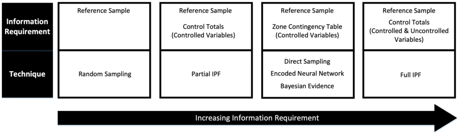
Varying information requirements of investigated methods.

Individuals are typically represented by categorical variables to describe their characteristics or attributes. Individuals with an identical set of characteristic categories belong to the same class or archetype. In the reference sample all characteristics are known, but in the zone contingency table, only some are known, termed as controlled variables, and others are desired, termed as uncontrolled variables. Each technique seeks to synthesize the complete archetype at the zone level based on the partial archetypes without introducing contradictory characteristic combinations.

These contradictory characteristics represent impossible combinations, known as structural zeros, which are distinct from improbable or non-stereotypical combinations that are not present in the reference sample data, known as sampling zeros.^8,25 The likelihood of sampling zeros increases with smaller populations or sample sizes or greater numbers of variables or categories.

The control totals are the aggregate column and row totals of a zone contingency table. The contingency tables and control totals are published but anonymizing techniques, such as value swapping, may result in total populations varying between alternative tables of the same zone. Typical contingency tables range from two to four variables, so multiple tables may be required to obtain the desired population characteristics. In IPF techniques the control totals must have consistent population totals, otherwise convergence may not be achieved. The following techniques have been selected for investigation.

3.1. Baseline sampling

The most simplified approach to population synthesis is to randomly draw records from the reference sample according to only the target zone’s population size. No consideration is given to the distribution of characteristics in the target population and instead selection is influenced by archetype frequency. This approach provides a minimum threshold which all alternative techniques should noticeably exceed, that is, perform better than a random guess.

3.2. Direct sampling

The controlled variables published in the contingency tables can be used to filter the reference sample records. This filtering provides a shortlist of records with both controlled and uncontrolled variables. This shortlist can then be sampled with replacement according to contingency table count. The repeated occurrence of archetypes in the shortlist forms a cumulative density function; more frequent archetypes are more likely to be sampled and is equivalent to the prior probabilities that are applied in the encoded ANN technique discussed later. Similar to other techniques, it cannot handle sampling zeros present in the reference sample and not in the target zone.

3.3. IPF

This commonly applied technique was developed with several variants. Detailed explanation of the iterative process and potential issues can be obtained from the literature.^16,26,27 The process is defined as having two stages of fitting and allocation. ⁶

During the fitting stage, a seed contingency table of constraint variables is iteratively reweighted against a set of marginal or control totals derived from the target zone. The iteration is repeated until the control totals of the seed across all constrained variables equal those of the target zone. The R package mipfp ²⁷ provides an IPF implementation and is used with an iteration limit of 100, as convergence is unlikely beyond this point, ²⁵ and the convergence tolerance is at the 1e-10 default value.

In the allocation stage, the fitted aggregate contingency table is converted into disaggregate individuals using integerization, selection, and placement steps, ²⁸ but the latter is not required to produce individuals. The integerization step is the rounding process to convert decimal cell values into integers and introduces the greatest error into the IPF process. The truncate replicate sample technique was shown to be the most effective ²⁹ and is used here.

We examined two implementations for alternative information scenarios. The technique full IPF uses constraint variables containing both controlled and uncontrolled variables. The technique partial IPF uses constraint variables containing only controlled variables; the uncontrolled variables are obtained from the reference sample after allocation as per the direct sampling technique, based on the assumption that uncontrolled variables are not independent of the controlled variables. ⁶ The best case for the partial IPF technique is using the control totals to accurately recover the original contingency table, as used in the direct sampling, encoded ANN and Bayesian evidence techniques. Therefore, the direct sampling technique is also the best-case scenario for the partial IPF technique.

3.4. Bayesian network

The BN method was proposed in Sun and Erath ¹⁹ to provide a probabilistic approach to population synthesis. The disaggregate individuals in the reference sample are used to construct a series of tree structures with associated probabilities. As illustrated in Figure 2, the network is represented by a graph where each node within represents a variable and directed edges between nodes show parent–child dependency. The probability distributions of edge instances describe the likelihood of a node selection given the combination of its parent variables.

Figure 2.

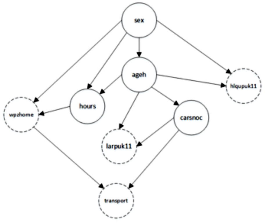
Directed acyclic graph (DAG) of controlled and uncontrolled variables based on an edges blacklist.

The approach proposed in Sun and Erath ¹⁹ is implemented using the R package bnlearn ³⁰ using the Akaike information criterion (AIC) ³¹ and Tabu search ³² to determine the most appropriate network structure, termed here as Bayesian evidence. A blacklist of forbidden graph edges is provided so that uncontrolled variables cannot be the parents of controlled variables. The population synthesis is performed using the controlled variable categories from the target zone as evidence for the network to produce a sample population that features both controlled and uncontrolled variables.

Individuals are randomly sampled from the sample population according to the controlled variable frequency count and added to the generated population. Individuals need to be filtered for undefined category values where the generation process has not produced a complete individual. ¹⁹ All controlled variable categories in the zone target must exist at least once in the reference sample, meaning sampling zeroes between them are not permitted.

3.5. ANNs

3.5.1. Overview of the ANN model

The application of ANNs as a machine learning technique to solve regression and classification problems has been applied in various domains with a variety of different structures being developed. The feed-forward or multilayer perceptron ANN structure can be used to solve log-linear models through nonlinear multinomial logistic regression. ANNs are inspired by the synaptic connections between neurons in the human brain to provide a network of parallel distributed processing units. ²²

A set of predictor variables, that is, controlled variables, are modeled as input nodes connected to layers of hidden units, consisting of weights and bias quantities, and then to response variables, that is, uncontrolled variables, in the output layer (see Figure 3). The connectivity between the hidden and output layers is through an activation function that is selected based upon the problem being solved. Although multiple hidden layers can be used, we opted for the common single layer ²¹ in order to reduce the computational complexity, as the intention of the work was to primarily investigate and compare the ANN approach with existing methods to establish a baseline and determine meaningful evaluation measures. Future work would investigate more complex structures and parameter tuning to improve performance.

Figure 3.

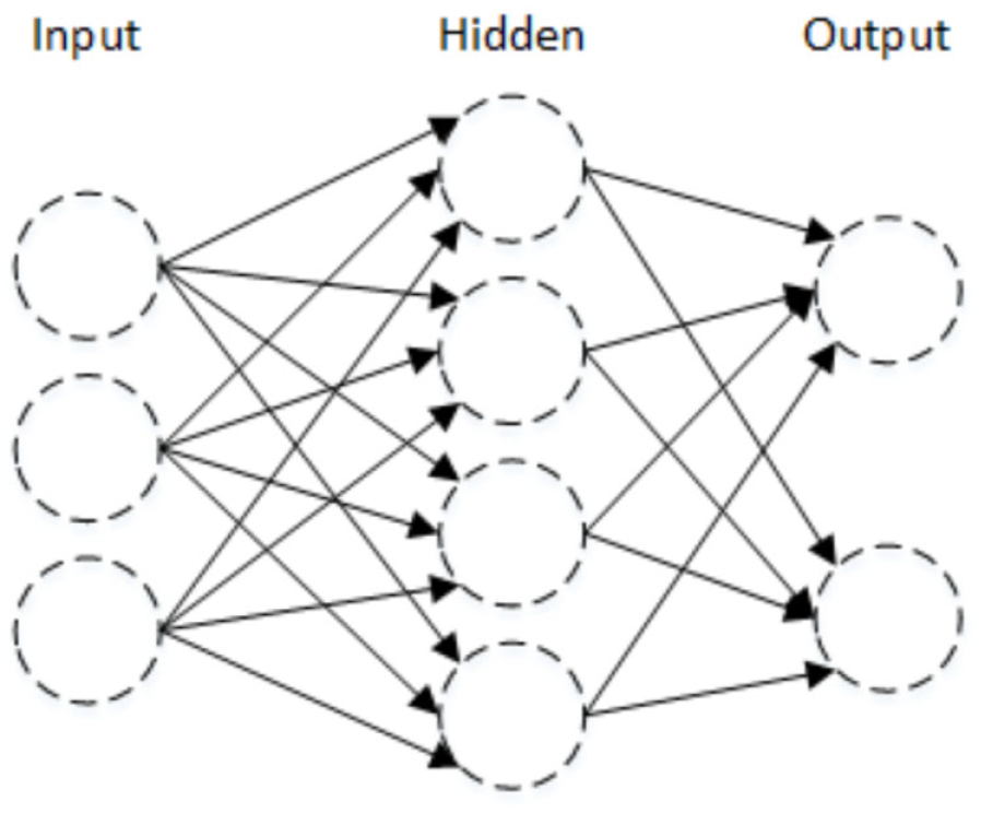
Example artificial neural network structure.

The activation function, or squashing function, limits the range of the hidden units’ output to a finite value. ²² In multinomial logistic regression, the softmax activation function, see Equation (1), provides an output response node probability of it being the correct class for the input values. The sum of these posterior probabilities across all the response nodes for the input values is equal to one as follows:

$$p\left(C_k|x\right)=\frac{exp(a_k)}{\sum _{j}exp(a_j)}$$

$$a_k=\ln p(x|C_k)p\left(C_k\right)$$

Equation (1): Softmax function.

The softmax function is the multiple input formulation of the S-shaped logistic sigmoid function which provides the nonlinear transformation of a value within a specified range 21. The output class can be selected either on the highest probability or by baseline sampling of these posterior probabilities, with the latter being chosen here to provide archetype diversity.

The input nodes can be a mix of continuous or categorical variables while output variables can be selected to be continuous or categorical. Therefore, a range of information can be utilized and predicted by the ANN. Continuous variables are typically adjusted to improve prediction through normalization or standardization techniques. The ability to utilize continuous variables for input variables means that quantization is unnecessary as required in IPF.

Similarly, categorical variables are subjected to encoding schemes. The encoding of these input and output variables splits them into a set of nodes with one node for each category in the variable. The commonly used dummy coding, ³³ also known as 1-of-C, 1-of-K, one-hot or treatment coding, uniquely encodes each category of the variable by assigning a single node the value one and the remainder zero.

The ANN is trained through a supervised learning approach using a training set of known predictor and response variables or can be unsupervised learning based only on the supplied data. The ANN is iteratively reweighted by supplying predictor variables and validating the accuracy of the response variable against the known results within the training set until predictive accuracy reaches a specified threshold or no longer improves. Once trained the ANN can be used to make predictions as to the value or classification of the output response variables based on the input predictor variables.

The structure of a multinomial ANN is to predict a single response variable with multiple categories. It is typical to synthesize populations that would require multiple response variables each with multiple categories. An approach to applying ANNs would be to train a separate network for each response or uncontrolled variable. These multiple ANNs would produce category predictions that are then combined to form the complete archetype. However, the sampling of the posterior probabilities could result in inconsistent archetypes being generated, that is, structural and sampling zeros. An area of future investigation is combining multiple networks using a mixture model approach.

3.5.2. Applying ANN for synthetic population generation

In this work a lossless encoding approach, potentially allowing the encoded variables to be fully recovered, is applied to group the categories across the multiple uncontrolled variables into a single variable category, termed as encoded ANN. Once prediction of the output variable category is complete the multiple categories of the uncontrolled variables are recovered. The Base64 encoding implemented by the R package base64enc ³⁴ was selected for the lossless encoding.

In Base64 encoding, a sequence of bytes, that is, 8 bits, is converted into a sequence of printable characters symbols. Each symbol encodes 6 bits with padding applied to ensure that the input sequence length is a factor of 6 and 8 as depicted in Figure 4. Two identical sequences of bytes will be encoded with the same unique sequence of symbols.

Figure 4.

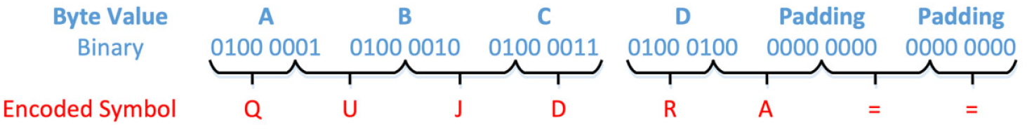
Encoding of 4 bytes to 8 Base64 symbols.

Each uncontrolled variable is encoded according to its numeric category value prior to applying contrast coding; see Table 1. In the examined dataset, the largest number of categories for any single variable in the investigated was 43, excluding the region label, and so all categories fit within a single byte. We adopted the implementation R package nnet that can be further reviewed in Ripley et al. ³⁵

Table 1.

Encoding of multiple characteristic variables to single Base64 encoded variable.

Characteristic variables				Encoded variable
A	B	C	D
0	0	0	0	AAAAAA ==
1	0	0	0	AQAAAA ==
0	1	0	1	AAEAAQ ==
1	1	1	0	AQEBAA ==

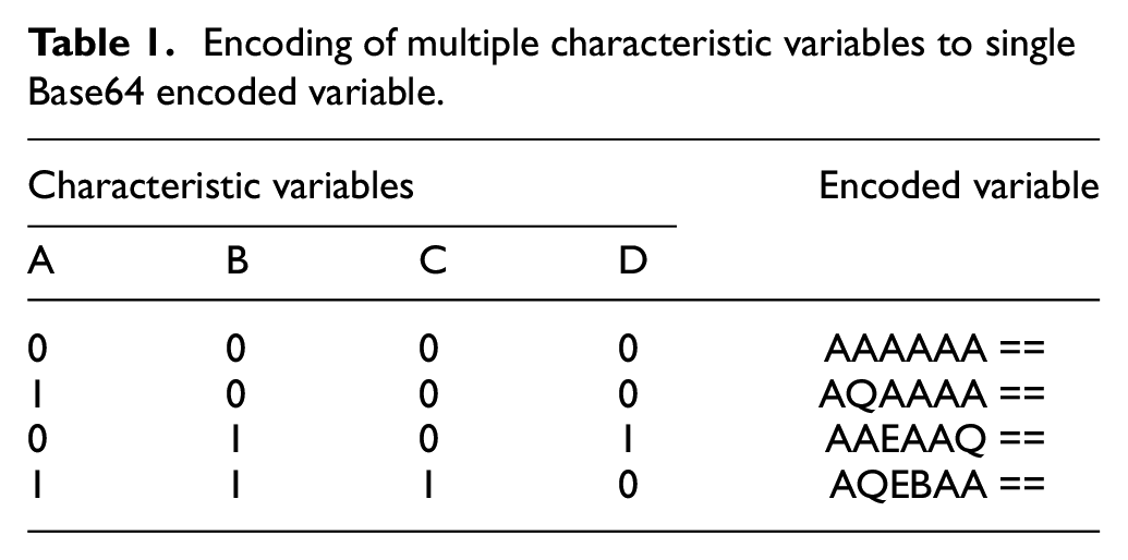
Encoding is performed on the reference sample to replace all the uncontrolled variables with a single encoded variable. Consequently, the multinomial neural network can be trained to predict the single response variable based upon the multiple controlled variables as input predictor variables. Once the response is provided, it is decoded into its equivalent categories of uncontrolled variables and combined with controlled variables to provide the generated individual.

The drawback of this approach is that the number of unique encodings (archetypes) representing the permutations of the uncontrolled variables in the reference sample, requires a large number of categories to be captured by the neural network in the response variable; see Figure 5. By applying the encoding to reduce the number of uncontrolled variables, it can be seen that the actual amount of the decision space being used by archetypes is much smaller than the full potential decision space of the variables; see Table 6.

Figure 5.

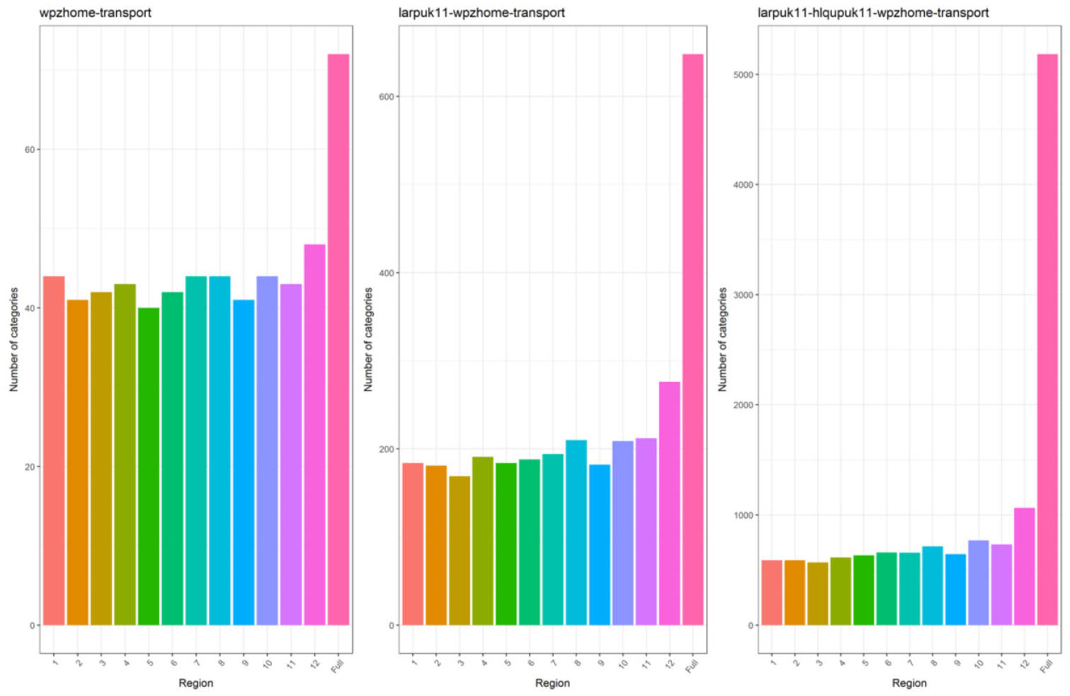
Number of categories for encoded uncontrolled variables across 2, 3, and 4 variables compared with full decision space of nonencoded uncontrolled variables.

An aspect of the ANN fitting process is the need for large numbers of samples to train the network weights. Archetypes that only have a single case are unlikely to be correctly trained in the network and can therefore be misclassified. In the examined dataset, the population size ratio to the large variety of potential archetypes means that reference samples are likely to contain archetypes with small counts. To address this issue the posterior probabilities produced by generative models or discriminative models, such as ANNs, can be adjusted by the prior probabilities based on Bayes theorem. ²¹

The original reference sample is rebalanced so that each unique archetype, across both controlled and uncontrolled variables, is replicated n times. This rebalanced dataset is then used to train the neural network and make predictions as to the posterior probabilities. The posterior probabilities are then divided by the replication number (n) and multiplied by the archetype frequency in the original reference sample. The resulting probabilities are then normalized to provide a probability distribution for sampling or selection.

The use of the prior probabilities has a masking effect on the posterior probabilities. Therefore, combinations of controlled and uncontrolled variables are given zero probability if they did not appear in the original reference sample. These prior probabilities are the same probabilities utilized in the direct sampling technique. This presents the opportunity of a single trained ANN being used on multiple regions, provided the balanced dataset contains all potential archetypes in the regions. The posterior probabilities of the generally trained ANN would be applied to each region’s own prior probabilities. This could enable a single national network to be constructed for each set of variables and applied to many regions, zones, or time periods.

The R package nnet ³⁵ was used for implementation with a single multinomial ANN being trained for each variable combination using the balanced reference samples. ³⁶ The controlled variables are used as predictors with encoded uncontrolled variables as the response and baseline sampling from the probability distribution. An authoritative recommendation for the number of replications in the balanced training set could not be found. Fifty replications were selected as a typical value for the occurrence of more frequent archetypes under various variable combinations and to avoid producing an excessively large training set.

Several parameters can be used to modify the neural network but only the number of iterations and number of weights have been adjusted in this investigation. Due to the number of categories in the encoded neural network approach, it is necessary to increase the maximum number of weights to fit the dimensionality, which has an impact on the speed of fitting. However, it should be noted that population synthesis can be regarded as an offline activity where users are waiting for rapid results and therefore processing time is a secondary concern to model accuracy.

The maximum number of weights was increased on a case-by-case basis as reported at runtime for the network. The maximum number of iterations was increased to 600 due to the increase in number of weights but again no definitive guidelines could be obtained. The weight decay parameter results in weight values that reduce toward zero unless sustained by the data and was found to improve generalization. ³⁷ Values of 0.0, 0.01, 0.02, 0.1, 0.25, and 0.5 were explored based upon suggested examples using 10-fold with three repeats cross-validation with the caret package ³⁸ with two and three uncontrolled variables. The weight decay 0.0 value typically resulted in the lowest logarithmic loss score and was applied for all scenarios.

4. Analytical measures

In order to evaluate the effectiveness of the different techniques in generating populations, both relative to each other and to the ground-truth population, it is necessary to apply goodness-of-fit measures. The following section discusses the error and similarity measures commonly used in population synthesis:

4.1. Error-based measures

These measures are applied to aggregate contingency tables of the populations between the target zone populations, termed actual, and generated synthetic population, termed predicted. It has been highlighted that no single measure has yet been derived, which provides a definitive test for goodness-of-fit and instead a variety of measures need to be considered. ²⁴

4.1.1. Total absolute error

The simplest metric to compare between the predicted and actual populations is to find the total difference in frequency for each archetype, see Equation (2), with a lower value being preferred (smaller is better). The total absolute error (TAE), or absolute error (AE), is the basis for several other metrics and gives the overall number of errors produced as follows:

$$\mathrm{TAE}=\sum _{i=1}^n(y_i-{\hat{y}}_i)$$

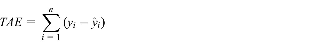
Equation (2): TAE formula of actual (y) against predicted ( $\hat{y}$ ) populations.

A drawback is that it does not consider the size of the populations or the number of variables and categories. This means that relative comparisons cannot be performed across different scenarios as populations or number of potential archetypes vary. ²⁴ An error in one archetype will be double counted as an error in another archetype. The lower bound of this measure is zero while the upper bound is twice the size of the population. Subsequent errors may mask each other if another error fills in for a shortfall.

4.1.2. RMSE

The RMSE, or root mean square deviation, measure is frequently used in population synthesis.^8,17,23,27 However, there has been discussion that the alternative MAE is preferable to RMSE and that the measure should no longer be used due to its ambiguous interpretation. ³⁹

The RMSE measure is the square root of the mean squared difference between the frequency counts of archetypes in the actual (y) and predicted ( $\hat{y}$ ) populations, where n is the number of potential archetypes in the contingency table, see Equation (3). This produces a decimal value with a result closer to zero being preferred (smaller is better) as follows:

$$\mathrm{RMSE}=\sqrt{\frac{\sum _{i=1}^n{(y_i-{\hat{y}}_i)}^2}{n}}$$

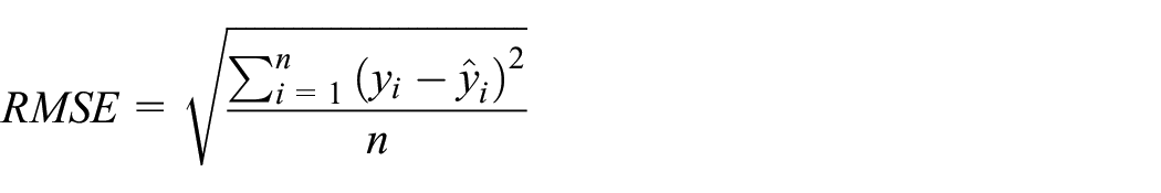
Equation (3): RMSE formula for actual ( $y)$ against predicted ( $\hat{y})$ populations.

The bounds of RMSE are not limited to the range of zero and one. Instead the lower bound is reported as being the MAE of the populations and the upper bound is the MAE multiplied by the square root of the potential archetypes ( $\mathrm{MAE}\times n^{\frac{1}{2}}$ ) (Willmott and Matsuura 2005). The usage of the number of potential archetypes (n) results in population sparsity and characteristic dimensionality having an impact on the measure. Smaller populations or higher dimensionality scenarios can be reported as closer to zero, and therefore appearing to have greater goodness-of-fit, despite the absolute or relative number of errors being the same. Therefore, comparison between scenarios is impaired.

4.1.3. Standardized RMSE

To compensate for differences in population sizes and variable dimensionality, the measure standardized root mean square error (SRMSE) was formulated in several ways as follows: ²³

$$\mathrm{SRMSE}=\frac{\mathrm{RMSE}}{\left(\frac{\sum _{i=1}^n{y}_i}{n}\right)}$$

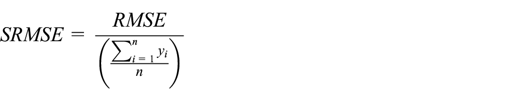
Equation (4): SRMSE formula of actual ( $y)$ against predicted ( $\widehat{y}$ populations.

This measure takes the RMSE measure and divides it by the mean actual population per entry; see Equation (4). It is suggested in the literature that the value of SRMSE is typically considered to range between zero and one. ⁴⁰ However, when the population is small relative to the number of potential archetypes then the mean population per entry is less than one. This has a multiplicative effect on the RMSE and could scale it above one. Also, the upper bound of RMSE can be greater than one; see previous section. Therefore, the upper bound is dependent upon the selected population and characteristic variables.

In addition, both RMSE and SRMSE give a heavier penalization of fewer large errors compared with many small errors. Table 2 shows an example of several identically sized populations with eight individuals across four archetypes (A, B, C, and D). In each case the actual population is unchanged while the predicted populations have the same number of errors (TAE), except in case #5. A decreasing RMSE can be seen as the errors are distributed more evenly despite the TAE remaining constant. Cases #3 and #4 have more errors than Case #5 and have introduced additional incorrect archetypes into the population but have equal or lower RMSE.

Table 2.

Example of variation in RMSE between many small errors and few large errors (2 d.p.).

Example	Actual				Predicted				RMSE	TAE	Pop Err	MAE
	A	B	C	D	A	B	C	D
#1	4	4	0	0	4	0	4	0	2.83	8	0.5	2
#2	4	4	0	0	2	2	4	0	2.45	8	0.5	2
#3	4	4	0	0	2	2	3	1	2.12	8	0.5	2
#4	4	4	0	0	2	2	2	2	2.00	8	0.5	2
#5	4	4	0	0	7	1	0	0	2.12	6	0.375	1.5

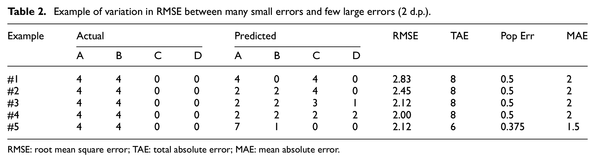
RMSE: root mean square error; TAE: total absolute error; MAE: mean absolute error.

The implications of this in population synthesis are that two populations could be generated that have the same number of errors, but due to the distribution one population is deemed preferable.

In some domains this penalty may be beneficial. However, a synthetic population that contains incorrect frequencies, but only correct archetypes, is preferred to another which contains incorrect archetypes of any frequency. In addition, the potential number of archetypes can quickly exceed the population size and so provide space for errors to be distributed thinly. This supports the earlier point made in the literature that RMSE and SRMSE should not be used for goodness-of-fit due to their ambiguous interpretation and behavior.

4.1.4. MAE

The MAE is a total error in the population (TAE) variant that compensates for variations in the contingency table size.^24,27 The TAE is divided by the potential number of cases (n), or archetypes, in the contingency table, as shown in Equation (5):

$$\mathrm{MAE}=\frac{\sum _{i=1}^n(y_i-{\hat{y}}_i)}{n}$$

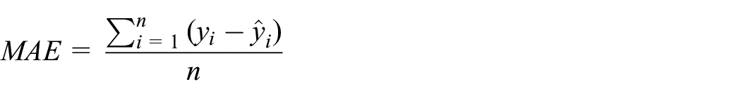
Equation (5): MAE formula of actual (y) against predicted ( $\hat{y}$ ) populations.

This approach gives a value that scales as the number of potential archetypes varies and does not penalize large errors in favor of small errors. It is proposed that this metric is used in favor of RMSE due to its unambiguous interpretation as a measure of average error magnitude. ³⁹ However, it should be noted that the metric does not compensate for variations in the total population size in different scenarios. While the lower bound is zero and a smaller value is preferred, the upper bound of the calculation is not fixed and will vary as the population size and number of archetypes vary. This makes it less suitable for comparison between populations without some form of standardization.

4.1.5. Population error rate

This measure is a combination of the standardized absolute error (SAE) ²⁴ and the classification error ⁴¹ metrics. The SAE metric is based upon the summation of the difference between actual (y) and predicted ( $\widehat{y}$ ) populations (TAE) divided by the total size of the actual population, see Equation (6), and has had several names as follows:^1,10

$$\mathrm{SAE}=\frac{\sum _{i=1}^n(y_i-{\hat{y}}_i)}{\sum _{i=1}^n{y}_i}$$

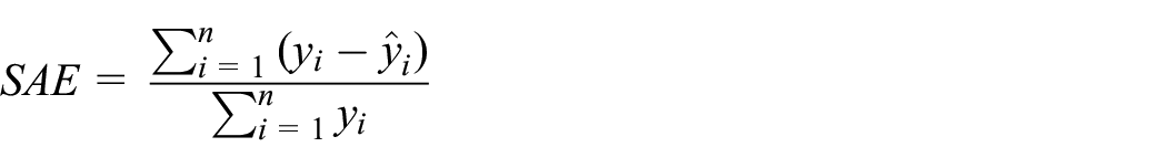
Equation (6): Standardized absolute error of actual (y) against predicted ( $\hat{y}$ ) populations.

The range of SAE, when the actual and predicted populations are identically sized, is from a lower bound of zero to an upper bound of two with a lower score indicating less error and so greater overlap between populations (smaller is better). The advantages of the SAE measure are that it enables comparison across population sizes and provides close approximations to several other goodness-of-fit measures that are more complicated to calculate. ²⁴

In addition, SAE does not give greater penalty to errors that are relatively large. Therefore, it provides an indication of the total errors in a population for comparison without favoring those populations where the errors are evenly distributed as in RMSE and SRMSE. However, its result ranges from zero to two due to the double counting attribute of the TAE.

The classification error measure removes this double counting by making a scalar adjustment by dividing by two; see Equation (7). The lower bound of this equation is zero and the upper bound is one with a value closer to zero being preferred (smaller is better). This has the advantage of being directly interpreted in relation to the size of the population as a score of 0.5 means that half the population are in error, as follows:

$$\mathrm{Population}\mathrm{Error}\mathrm{Rate}=\frac{\sum _{i=1}^n(y_i-{\hat{y}}_i)}{2\sum _{i=1}^n{y}_i}$$

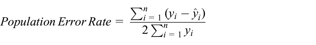
Equation (7): Population error rate of actual (y) against predicted ( $\hat{y}$ ) populations.

This formulation is described as the percentage classification error (% CE) ⁴¹ and in inverse form as the proportion of good prediction (PGP). ⁴² The term population error rate has been applied to make a distinction from the classification error ⁴³ used for model accuracy, where a direct response is received to an input, which is not discussed as it cannot be applied to IPF methods.

4.2. Similarity measures

The previous error-based measures consider the degree of difference between the archetype counts of the actual and predicted populations. An alternative perspective is to consider the similarity and difference in the archetypes present in populations. The techniques that provide more representative range of archetypes from the target population, whether including correct or excluding incorrect archetypes, should be preferred.

4.2.1. Jaccard similarity coefficient

An established measure in set theory for determining the similarity between sets is the Jaccard index or Jaccard similarity coefficient. ⁴⁴ This measure is calculated by dividing the size of the intersection of the two sets by the size of the union of the two sets; see Equation (8) and Figure 6. The resulting value ranges from zero to one inclusively with a larger value indicating greater set similarity (Bigger is better) as follows:

$$J(A,B)=\frac{|A\cap B|}{|A\cup B|}$$

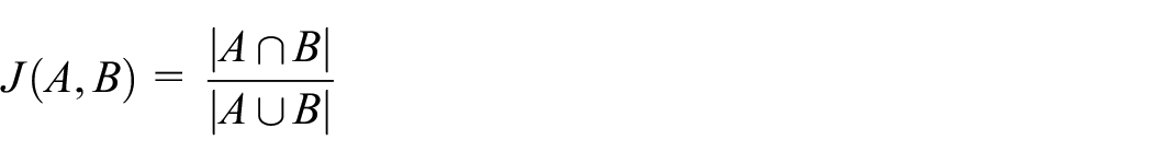
Equation (8): Jaccard Index equation for two sets: A and B.

Figure 6.

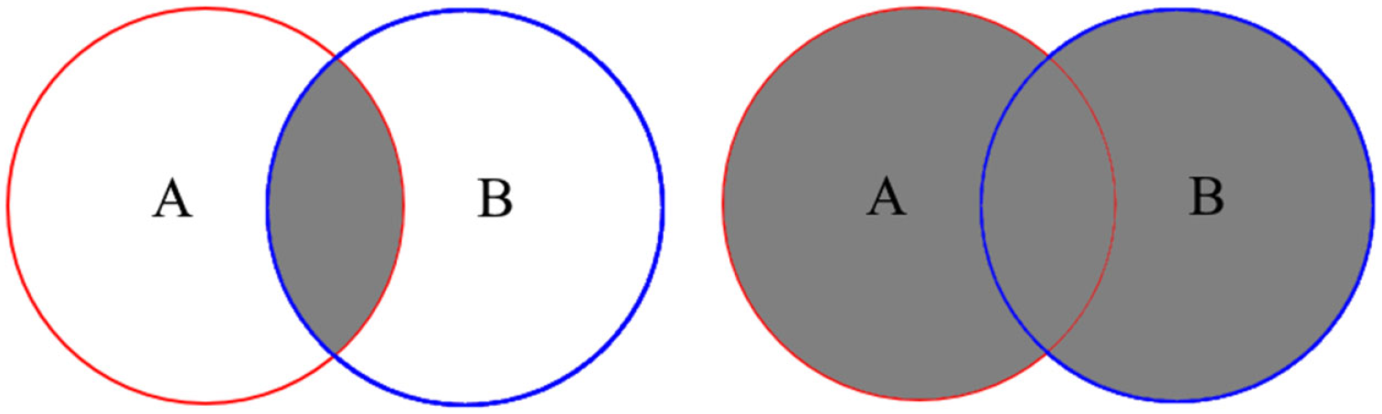
Intersection (left) and union (right) of two sets: A and B.

This measure is not influenced by the relative sparsity caused by the changes to the variable combinations as has been identified previously for the RMSE and MAE measures.

4.2.2. Intersection rate

To expand upon the Jaccard coefficient, it is necessary to focus on the intersection aspect to examine the synthesis of archetypes in the actual population into the predicted population. By dividing the intersection between predicted and actual populations by the number of archetypes in the actual population a standardized measure can be obtained, shown in Equation (9) as follows:

$$\mathrm{Intersection}\mathrm{Rate}(P,A)=\frac{|P\cap A|}{\left|A\right|}$$

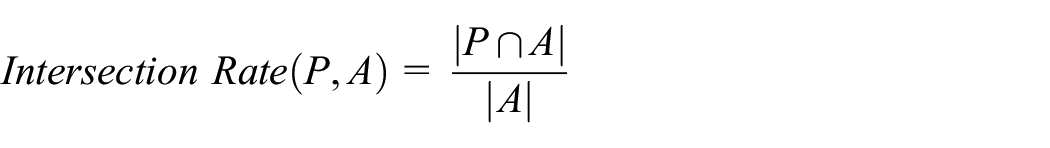
Equation (9): Intersection rate between predicted (P) and actual (A) populations.

The score ranges from zero to one with the upper bound indicating that a large proportion of desired archetypes are present in the predicted population (Bigger is better).

4.2.3. Difference rate

The counterpoint to examining the intersection is to examine the difference in archetypes between the actual and predicted populations, using the relative complement or asymmetric difference, shown in Equation (10) and Figure 7 as follows:

$$B\backslash A=\{x\in B|x\notin A\}$$

Equation (10): Set relative complement.

Figure 7.

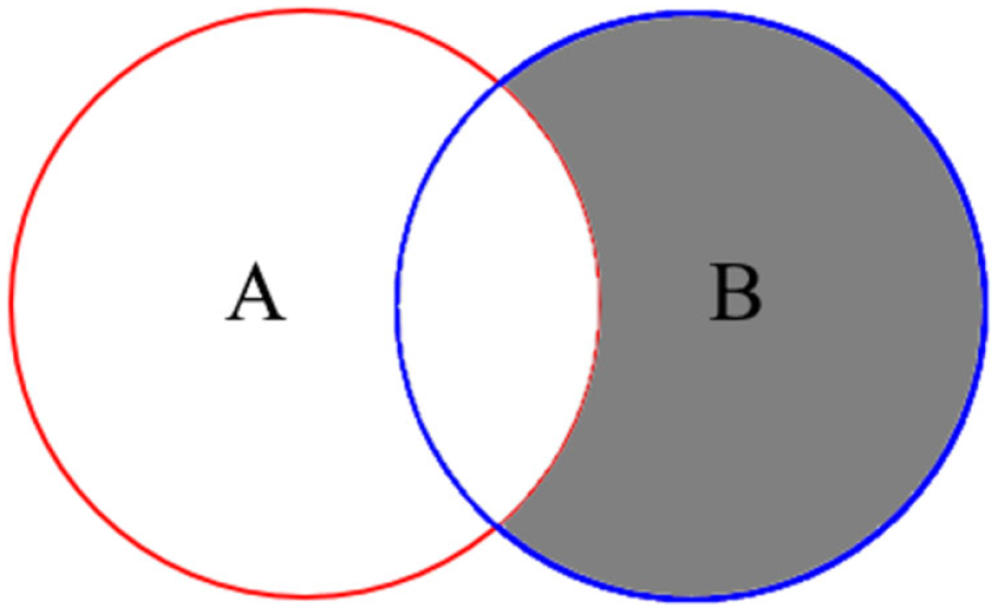
Relative complement of two sets: A and B.

This measure can be applied between the predicted (P) and actual (A) populations, see Equation (11), to show archetypes that would not be expected to be present as follows:

$$\mathrm{Difference}\mathrm{Rate}(P,A)=\frac{\left|\{x\in P|x\notin A\}\right|}{\left|P\right|}$$

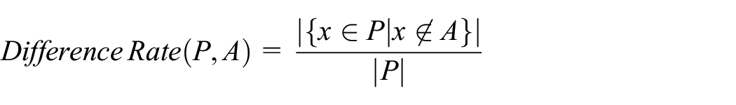
Equation (11): Difference rate between predicted (P) and actual (A) populations.

Alternatively, it can be applied to the predicted (P) and reference sample (R) populations, see Equation (12), to show archetypes that have been generated by the technique. Absence from the reference sample indicates incomplete sampling of the actual population, that is, sampling zeroes, or inconsistent archetypes that should not logically or practically exist, that is, structural zeroes, as follows:

$$\mathrm{Difference}\mathrm{Rate}(P,R)=\frac{\left|\{x\in P|x\notin R\}\right|}{\left|P\right|}$$

Equation (12): Difference rate between predicted (P) and reference sample (R) populations.

When the reference sample (R) fully represents the archetypes in the actual population (A) there are no sampling zeroes, that is., differences are structural zeroes. In both formulations of the difference rate, the measure is standardized permitting comparison between scenarios. A smaller value closer to zero being more desirable while the upper bound of one would indicate complete difference (smaller is better).

5. Compilation of the synthesis dataset

This section outlines the compilation of the initial dataset from the UK Census data, describes its characteristics, and outlines the experimental setup.

5.2. Dataset structure and processing

The objective of population synthesis is to produce a representative population of individuals based on partial and incomplete information about the population. There are two primary types of datasets used in the process:

• Reference sample: Disaggregate anonymized individuals sampled from large geographic regions; for example, UK Census Microdata, US PUMS;

• Zone Contingency Tables: Aggregate characteristic counts for small geographic zones.

The examined dataset is the UK Census 2011 Individuals Local Authority Microdata, ⁴⁵ which covers 265 Local Authority areas that range in size from 6019 to 54,396 records (mean 10,748, SD 4772). Each area is a 5% sample of the population and contains anonymized individuals described by 121 categorical variables. The variables are grouped into conceptual levels including person, family, or household.

Each Local Authority area can be further subdivided into a varying number of zones within a geographic hierarchy based upon population distribution. Complete individual records are not published at zone level, which would remove the need for population synthesis, to preserve anonymity from the small numbers in each zone. Yet, ground-truth populations are required to evaluate technique effectiveness and so zone-level populations were constructed from the microdata.

The Local Authority areas in the dataset each form a reference sample region. These were separated into 12 quantiles according to population size. One region from each quantile was randomly selected for experimentation. Only the region closest to the mean population of the dataset is reported here for brevity. A full-sized region population was created by duplicating the region reference samples 20 times, that is, reversing the 5% sample.

The full-sized region was randomly sampled without replacement to construct zones at three geographic hierarchy levels. These zones have complete population characteristics to measure fit and derive contingency tables and control totals. This process was repeated 10 times for each geographic hierarchy level with one zone retained each time.

There are three influencing consequences of this approach upon the experiments. First, the zones do not reflect actual population structures at the subregion level. Second, the zones are always subsets of the records present in the region reference sample, that is, no sampling zeros; the presence of sampling zeros inhibits some techniques. Finally, any control totals drawn from the zones will have balancing population totals between tables; a requirement for IPF methods and not guaranteed in practical datasets.

5.1.1. Geographic hierarchy

The geographic hierarchy allows the decomposing of areas into a set of smaller geographic areas. The usage of smaller geographic areas enables finer granularity in later traffic simulation. The terms region and zone are used to distinguish between areas at different levels of the hierarchy relative to each other. Regions consist of large geographic areas such as a province, county, or city that are composed of many smaller zones. Zones may be a few streets in dense urban areas or larger in rural districts. An area could function as both a zone of a region and itself have zones.

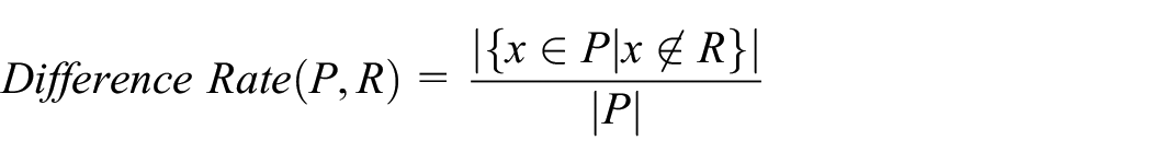
In the dataset, the composition and boundaries of each area are determined by the minimum and maximum population and household thresholds; ⁴⁶ see Table 3. Several output areas fit within the boundary of a lower layer super output area (LSOA), which is one of several within a middle layer super output area (MSOA) and so on. The level of detail published in datasets typically decreases moving down the hierarchy to smaller populations.

Table 3.

UK Census 2011 population and household hierarchy thresholds.

UK Census 2011 Hierarchy	Population		Households
	Minimum	Maximum	Minimum	Maximum
Output area	100	625	40	250
LSOA	1000	3000	400	1200
MSOA	5000	15,000	2000	6000

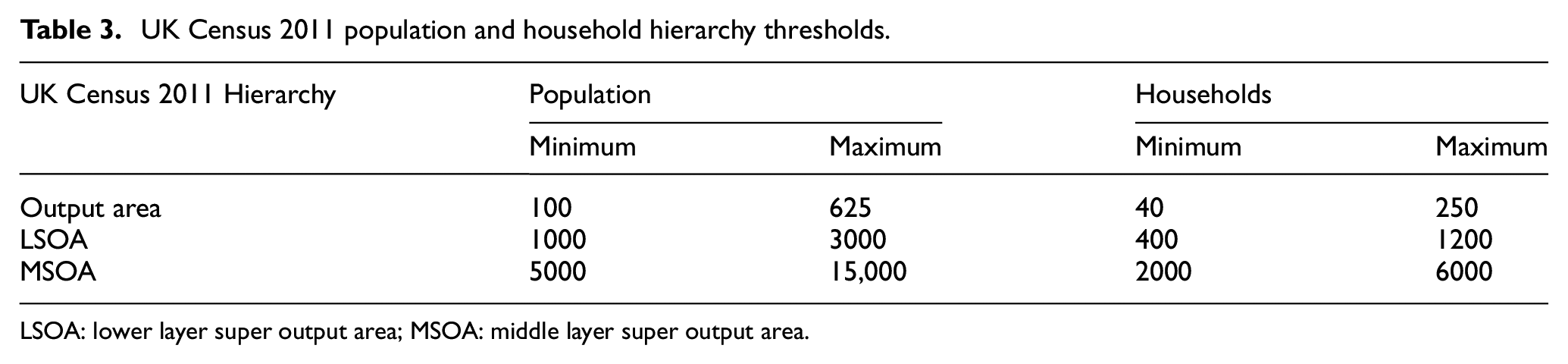
LSOA: lower layer super output area; MSOA: middle layer super output area.

As listed in Table 4, five zone sizes were used in the experiments, relatable to the UK Census 2011 hierarchy, to derive equally distributed thresholds. The zone counts for each size were based on calculating the midpoint population for each hierarchy level. This was then divided into the mean region population count, rounded to appropriate nearest values, and compared with the threshold levels for the smallest and largest regions in the full dataset.

Table 4.

Zone sizes selected for geographic hierarchy for investigation.

Zone count	UK Census 2011 hierarchy approximate Level	Region sample size (2 d.p.)	Population count
1200	OA: Lower Bound	0.08%	169
600	OA: Upper Bound	0.17%	338
300	N/A	0.33%	676
100	LSOA	1.00%	2030
20	MSOA	5.00%	10,150

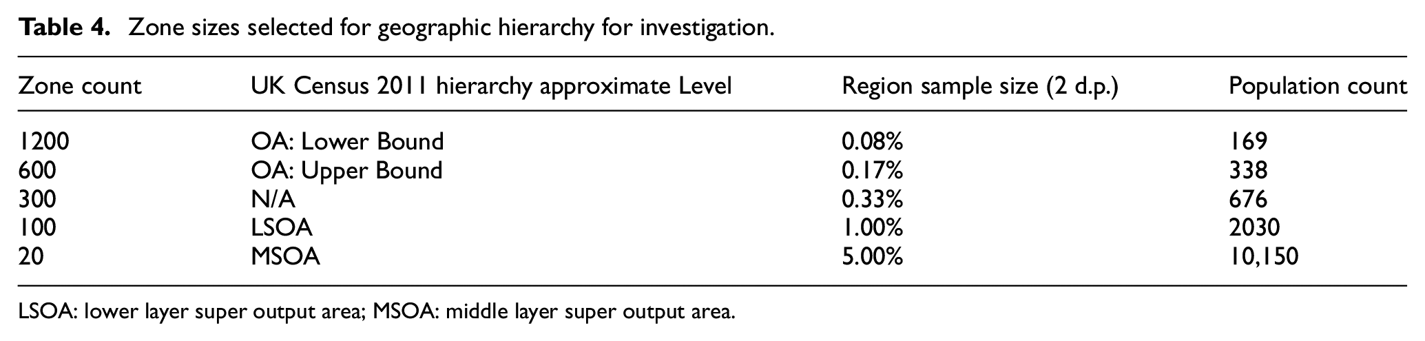
LSOA: lower layer super output area; MSOA: middle layer super output area.

The zone counts comply with the population thresholds for all but the largest 30 of the 265 regions. The 300 count was included as an interim step between the OA and LSOA sizes while the 1200 count was included to provide population sizes closer to the lower range of the Output area threshold for smaller and medium sized regions.

5.1.2. Characteristic selection: controlled and uncontrolled variables

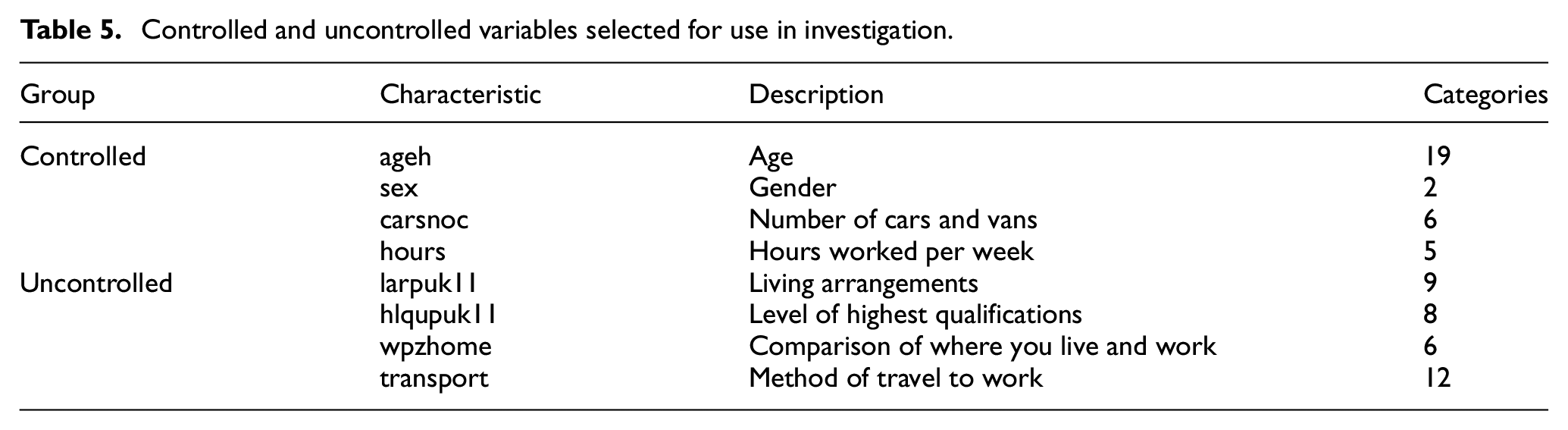
The reference samples contain 121 variables which have been reduced down to eight from the person conceptual level as illustrated in Table 5, based on relevance to the transport domain and previous usage.^8,19,47 These were divided into controlled and uncontrolled variable sets. Only Age and Gender had complete entries with all other empty entries being encoded as an “unknown” category to ensure consistent handling by all techniques.

Table 5.

Controlled and uncontrolled variables selected for use in investigation.

Group	Characteristic	Description	Categories
Controlled	ageh	Age	19
	sex	Gender	2
	carsnoc	Number of cars and vans	6
	hours	Hours worked per week	5
Uncontrolled	larpuk11	Living arrangements	9
	hlqupuk11	Level of highest qualifications	8
	wpzhome	Comparison of where you live and work	6
	transport	Method of travel to work	12

Typical published contingency tables for the UK Census ⁴⁵ contain between two and four characteristic variables. The controlled variables in Table 6 were selected from the UK Census reference information based on relevance to the transport domain. The combinations were examined to vary the amount of input information available to the techniques against single combinations of two to four uncontrolled variables for outputs. Each combination of controlled and uncontrolled variables results in a varying combined observation and decision space. The observation space comprises the controlled variables that are held constant throughout the synthesis process; the decision space comprises the uncontrolled variables.

Table 6.

Observation and decision space sizes for variable combinations.

Controlled variable combination	Observation space	Uncontrolled variable combination
		wpzhome-transport	larpuk11-wpzhome-transport	larpuk11-hlqupuk11-wpzhome-transport
		Decision space
		72	648	5184
		Combined space (Observation & Decision)
sex-hours	10	720	6480	51,840
sex-carsnoc	12	864	7776	62,208
carsnoc-hours	30	2160	19,440	155,520
ageh-sex	38	2736	24,624	196,992
sex-carsnoc-hours	60	4320	38,880	311,040
ageh-hours	95	6840	61,560	492,480
ageh-carsnoc	114	8208	73,872	590,976
ageh-sex-hours	190	13,680	123,120	984,960
ageh-sex-carsnoc	228	16,416	147,744	1,181,952
ageh-carsnoc-hours	570	41,040	369,360	2,954,880
ageh-sex-carsnoc-hours	1140	82,080	738,720	5,909,760

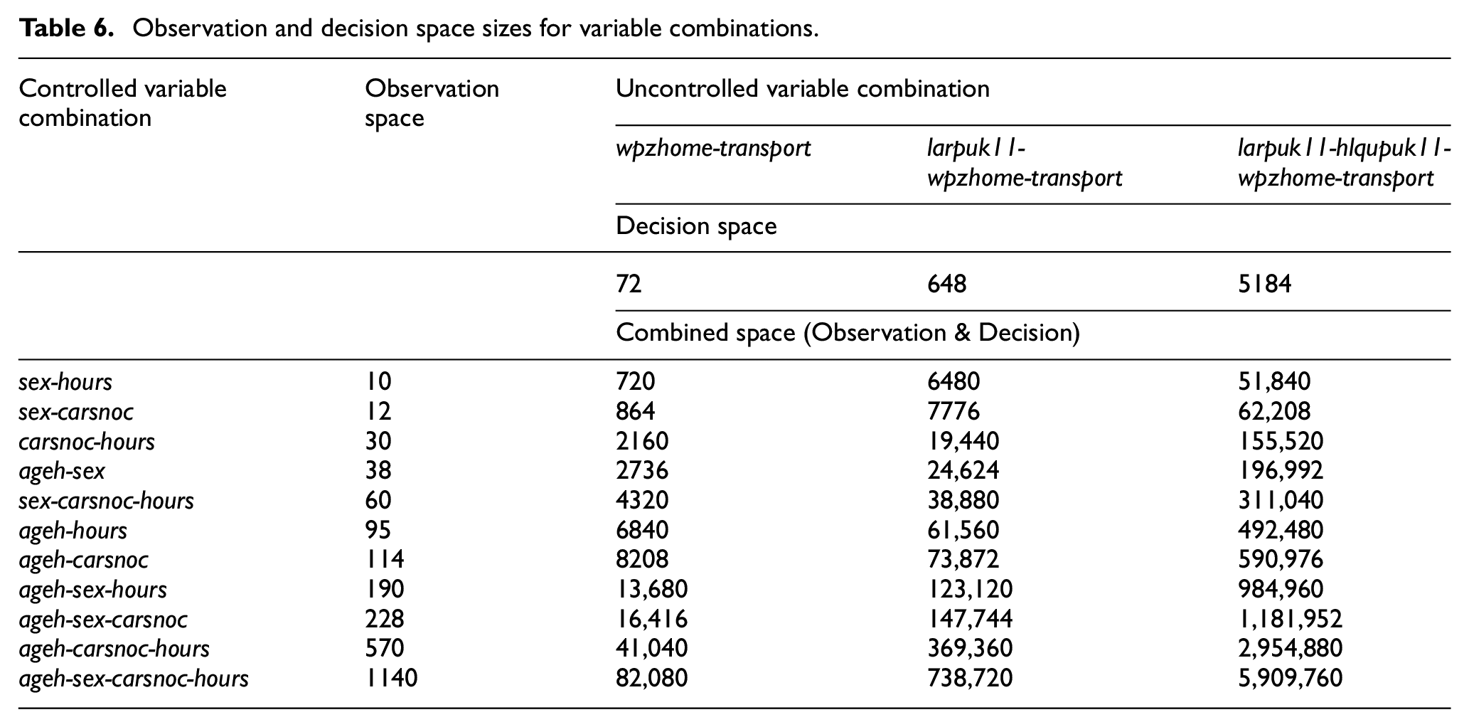
The combined space size is the number of potential archetypes and is used in certain error metrics. The potential archetypes rise very quickly as additional variables and numerous category variables are included. Sparse coverage of archetypes will arise given the largest zone size for the largest region has a population size of 54,396 records. Therefore, goodness-of-fit metrics that cannot handle sparse contingency tables, such as Pearson chi-squared test, are generally inappropriate. ²⁴

6. Analysis of the experimental results

This section presents and discusses our experimental results. The first subsection assesses the effectiveness of the deployed metrics in evaluating the error in the synthesized population in terms of coverage divergence and distribution of archetypes. The second subsection evaluates the performance of the developed ANN approach against traditional population synthesis techniques.

6.1. Evaluating the error metrics

The comparison of the three error metrics of SRMSE, MAE, and population error rate revealed several interesting findings. Figure 8 shows the simplest scenario of the largest zone count 20 with ascending observation space and fixed decision space of two output variables. The SRMSE and MAE measures utilize both the observation and decision space. Therefore, it is unclear whether the change in controlled variables is having a positive or negative effect on the error rate as it would need to exceed the relative change in size of the combined space.

Figure 8.

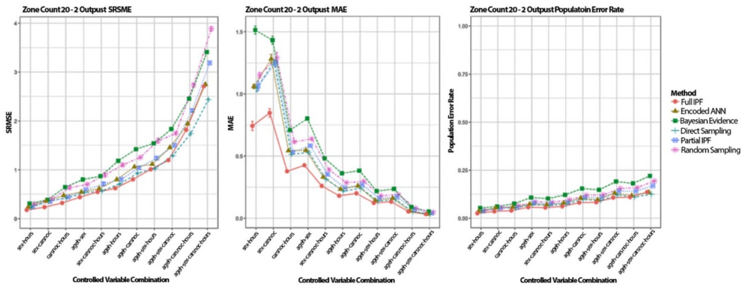
SRMSE, MAE, and population error rate across variable combinations in zone count 20 for 2 outputs (smaller is better and standard error bars in all cases).

In SRMSE, the size of the combined space has a multiplicative effect when a sparse population is used, as seen by the rapidly rising values as the space increases. We concluded that there are two to four times, as many errors between variable combinations cannot be drawn. In MAE, a similar but inverse effect is seen where each error becomes proportionally less important despite the populations being of the same size. In the population error rate metric, the deterioration can be clearly noticed as the observation space increases. This is to be expected as the number of archetypes is increasing and there are more potential mappings from controlled to uncontrolled variables. It is also possible to draw the conclusion that the population error rate stays below 25% for all the techniques in this zone count and the relative performance between combinations.

The ageh-sex-carsnoc-hours, and other variable combinations, demonstrate the heavier penalty for larger errors in the SRMSE metric. Both MAE and population error rate use the TAE and show Bayesian evidence with the greatest error rate. However, the SRMSE shows baseline sampling as a higher error rate. The number of errors in a population and their distribution are both important factors in the effectiveness of a technique, which RMSE and SRMSE obscure.

Examining this single variable combination across multiple zone sizes shows similar issues, as can be seen in Figure 9. As the combined space is fixed and the population size is decreasing from zone count 20 through 1200, it is expected that errors increase in smaller populations as each becomes more significant. However, the SRMSE has an increasing trend that could be attributed to increasing error rate or the decreasing population size. The MAE has a declining error rate suggesting that the techniques are becoming more effective. Instead, the significance of each error is declining as the emptiness of the variable space overwhelms the population size and each error is proportionally less significant. The population error rate shows that as the population decreases, the errors and thier weights increase. Therefore, the relative size of the variable space to the number of errors is not a factor in the metric.

Figure 9.

SRMSE, MAE, and population error rate for ageh-sex-carsnoc-hours with two outputs across zone sizes.

As can be observed in Figure 10, increasing the number of output variables increases the decision space and the number of archetypes present in the populations. For both SRMSE and MAE the relative values are noticeably different; therefore, direct comparison to the previous scenario becomes difficult while population error rate retains the unit interval. Comparison between the increasing SRMSE and decreasing MAE gives a contradictory view of error rate between scenarios when greater archetype diversity would predict an increase.

Figure 10.

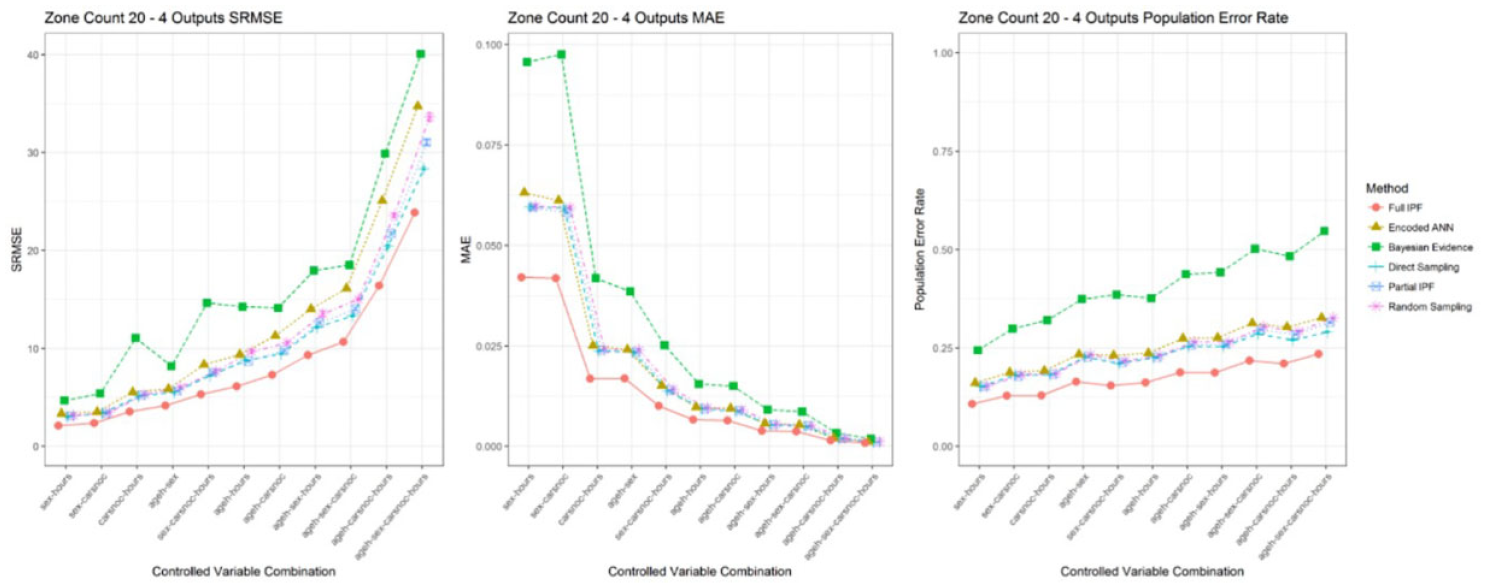
SRMSE, MAE, and population error rate across variable combinations in zone count 20 for 4 outputs (smaller is better and standard error bars in all cases).

The transition between variable combinations for sex-carsnoc and carsnoc-hours as the observation space increases from 864 to 2160, triggers a step change in error rate for the MAE metric across all techniques; the increase in potential archetypes does not directly correspond to an actual increase, indicating that the response is a characteristic of the measure rather than techniques being disrupted by greater archetype diversity. The population error rate shows more modest changes, perhaps better reflecting the actual increase in archetype numbers, and indicates that the increase in decision space has caused an overall increase in errors.

Decreasing the population size from zone count 20 to 100 causes changes to axis scaling for SRMSE and MAE, as shown in Figure 11. Relative comparisons for SRMSE are difficult between zone count scenarios. Changes in error rate could be attributed to the change in observation space size, population size, or both. The MAE and population error rate are not impacted by this change. However, the MAE still shows the contradictory decline as each error has a smaller significance as the combined variable space increases. The population error rate, characterized with disregard for the variable space scalability over a consistent and fixed range, makes comparisons between scenarios easier. However, as discussed previously this technique does not demonstrate the coverage of archetypes in the population and similarity between populations.

Figure 11.

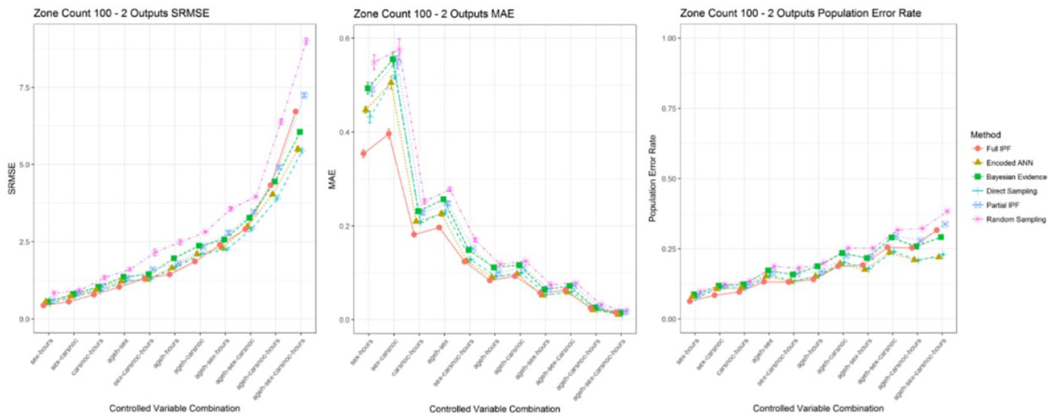
SRMSE, MAE, and population error rate across variable combinations in zone count 100 for 2 outputs (smaller is better and standard error bars in all cases).

The proposed metric of the Jaccard similarity coefficient, supported by the intersection rate and difference rate, is intended to provide a measure for population archetype coverage and explain the source of errors. Applied to the initial scenario of zone count 20 with two outputs as depicted in Figure 12, the pattern of error rate performance is reflected in the Jaccard similarity coefficient. The full IPF technique, ranging between 0.75 and 0.91, has consistently the highest values which correspond to the lower population error rate (Figure 8). The intersection rate, which shows the proportion of archetypes that should be present in the synthesized population, is very high, ranging between 0.94 and 1.0, and noticeably exceeds all the other techniques.

Figure 12.

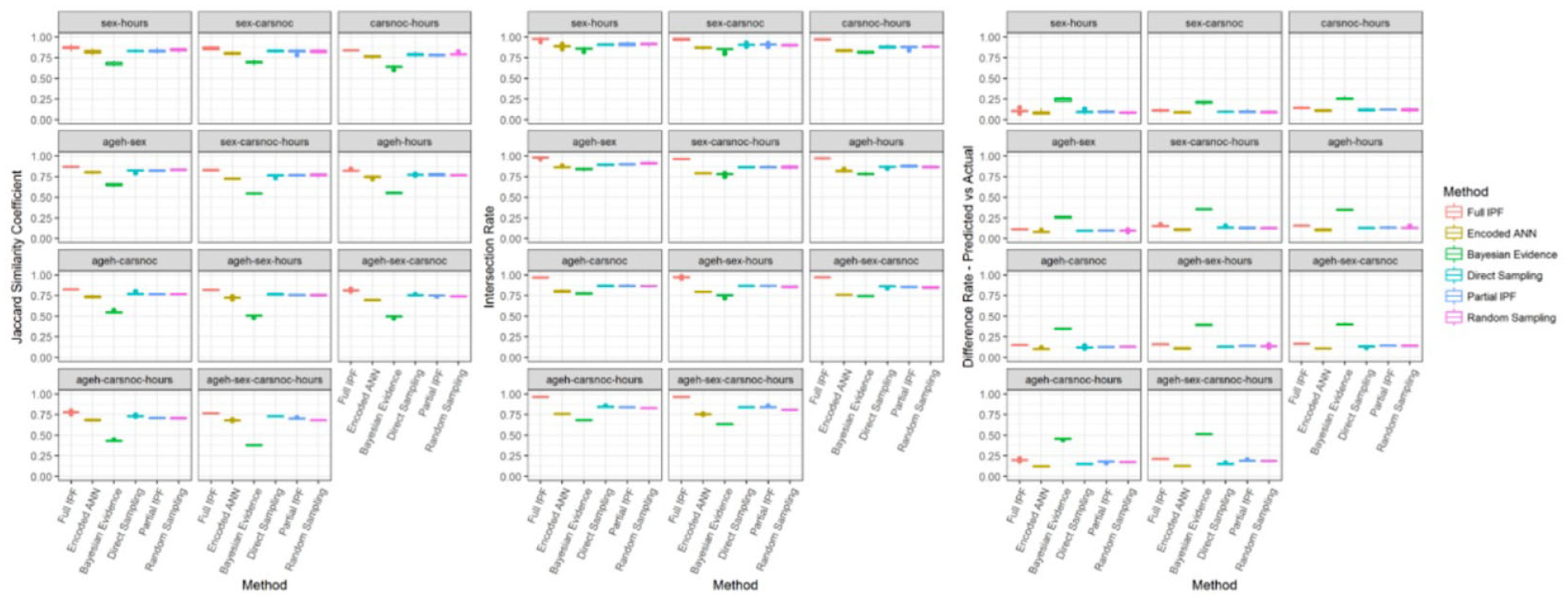
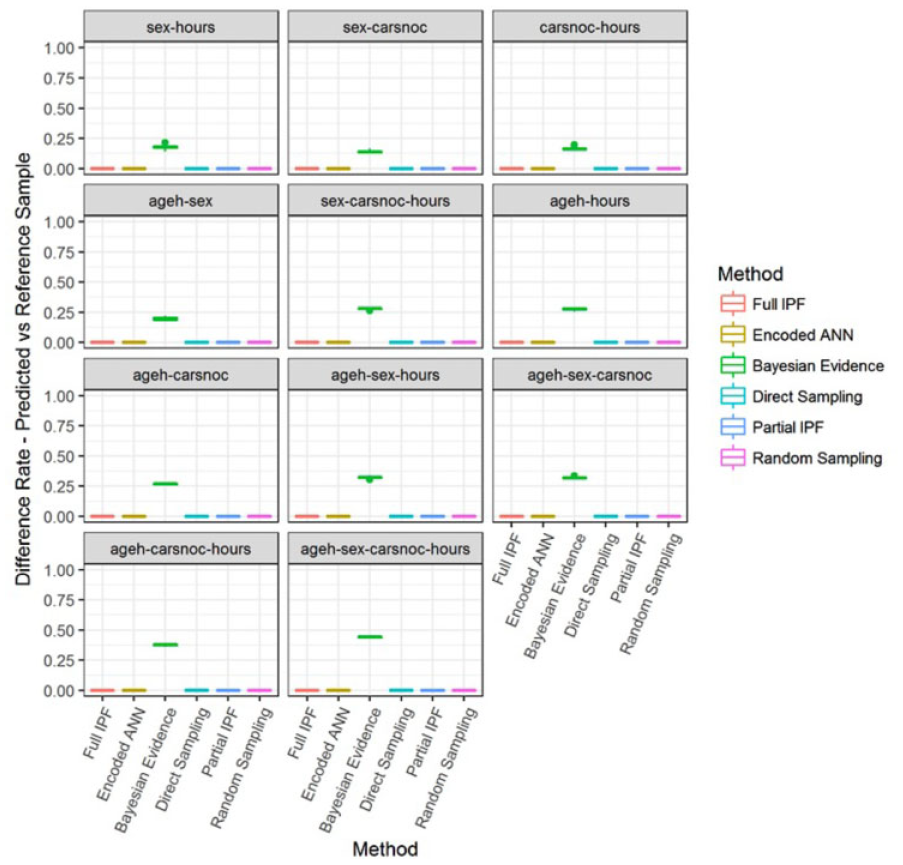
Jaccard similarity coefficient (bigger is better), intersection rate (bigger is better), and difference rate—predicted versus actual (smaller is better) in zone count 20 for two outputs.

However, the source of errors in the synthesized population can be seen to be not just the higher or lower distribution of these correct archetypes, but the inclusion of incorrect archetypes, as shown by the difference rate for predicted against actual populations. The full IPF technique has the second highest difference rate in all the variable combinations. Therefore, while the full IPF technique in this scenario provides excellent coverage of the correct archetypes, it is also including more incorrect archetypes than most other techniques.

The encoded ANN technique also demonstrates the importance of considering the error rate alongside the similarity metrics. As observed in Figure 8, in the ageh-sex-carsnoc-hours variable combination for two outputs and zone count 20, the encoded ANN achieves the second lowest population error rate. However, its mean intersection rate is the second worst while the mean difference rate—predicted versus actual is the best, as depicted in Figure 12. This means that the technique provides quite narrow coverage by synthesizing less archetypes than the other techniques, as demonstrated in part by the second worst Jaccard similarity coefficient. Therefore, while the relative error rate is low, there is less diversity in the population, which depending on usage may or may not be an advantage.

The final aspect of these metrics is to consider the inclusion of archetypes that were not present in the reference sample; see Figure 13. This metric is not important for those techniques which are based on cloning from the reference sample, such as IPF, direct sampling, and baseline sampling, as they cannot produce archetypes from outside that set. Similarly, the encoded ANN technique cannot produce archetypes from outside the reference sample set as the use of prior probabilities, to rebalance the samples for training, masks out inappropriate combinations.

Figure 13.

Difference rate—predicted versus reference sample (smaller is better) in zone count 20 for two outputs.

The Bayesian evidence technique as a generative model produces a joint distribution of the variables that can introduce new archetypes. This can be seen by the difference rate—predicted versus reference sample metric, which is a subset of the difference rate—predicted versus actual in these experiments. Most of the errors synthesized by the Bayesian evidence technique in this scenario are archetypes that do not feature in either the target actual population or the reference sample. This suggests that the learning process has not been effective on the dataset. However, due to its usage of the reference sample, which is available in practical conditions unlike the target actual population, it would be possible to identify and reject these inappropriate archetypes at runtime and resample.

6.2. Evaluating the performance of the ANN approach

The performed experiments allow the examination of the results in three key ways: controlled variables forming the observation space; uncontrolled variables forming the decision space; population size through zone counts. Examination of techniques is undertaken across the three uncontrolled variable sizes of two, three, and four outputs and against the largest (20), medium (300), and smallest (1200) zone counts. A focus is placed upon the population error rate for the reasons highlighted in the previous section.

In the smallest decision space scenario of two outputs for zone count 20 as recorded in Figure 14, the encoded ANN performs behind the full IPF and direct sampling techniques in several of the controlled variable combinations. However, as the variable combinations are increased the technique overtakes the full IPF technique in relative performance.

Figure 14.

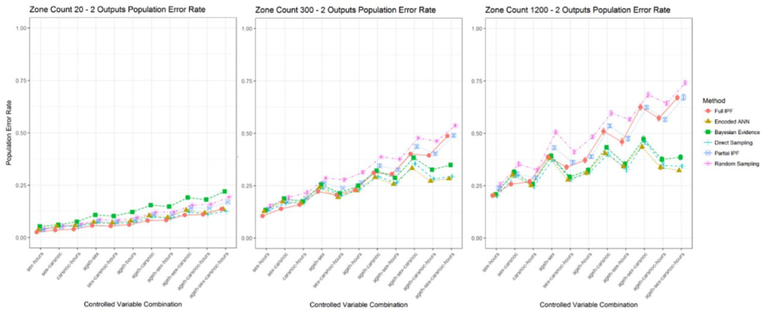
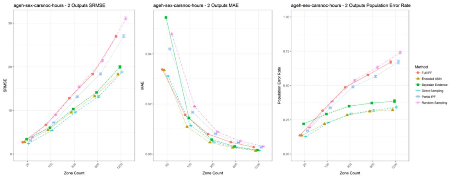
Population error rate across zone counts for two outputs (smaller is better).

The full IPF technique performs well with a small observation space and achieves the lowest overall population error rate in these simplest scenarios. The performance advantage of encoded ANN is witnessed as the population size becomes sparser in the zone count 300 and zone count 1200 scenarios as recorded in Table 7. It can also be observed that the full IPF technique, along with partial IPF and baseline sampling, display an upward trend in error rate while direct sampling, encoded ANN, and Bayesian evidence show stabilization and even declines in error rates.

Table 7.

Ranking of methods by smallest population error rate for two outputs.

Method	Zone count	Mode rank	1st/2nd (%)	Rank frequency
				1st	2nd	3rd	4th	5th	6th
Full IPF	20	1st	91	9	1	1	0	0	0
	300	1st & 4th	46	4	1	2	4	0	0
	1200	4th	18	1	1	1	6	2	0
Encoded ANN	20	3rd	9	0	1	8	2	0	0
	300	1st	82	7	2	1	1	0	0
	1200	1st	82	5	4	2	0	0	0
Bayesian evidence	20	6th	0	0	0	0	0	0	11
	300	4th	0	0	0	4	6	1	0
	1200	3rd	0	0	0	8	2	1	0
Direct sampling	20	2nd	91	2	8	1	0	0	0
	300	2nd	73	0	8	3	0	0	0
	1200	2nd	100	5	6	0	0	0	0
Partial IPF	20	4th	9	0	1	1	9	0	0
	300	5th	0	0	0	1	0	10	0
	1200	5th	0	0	0	0	3	8	0
Baseline sampling	20	5th	0	0	0	0	0	11	0
	300	6th	0	0	0	0	0	0	11
	1200	6th	0	0	0	0	0	0	11

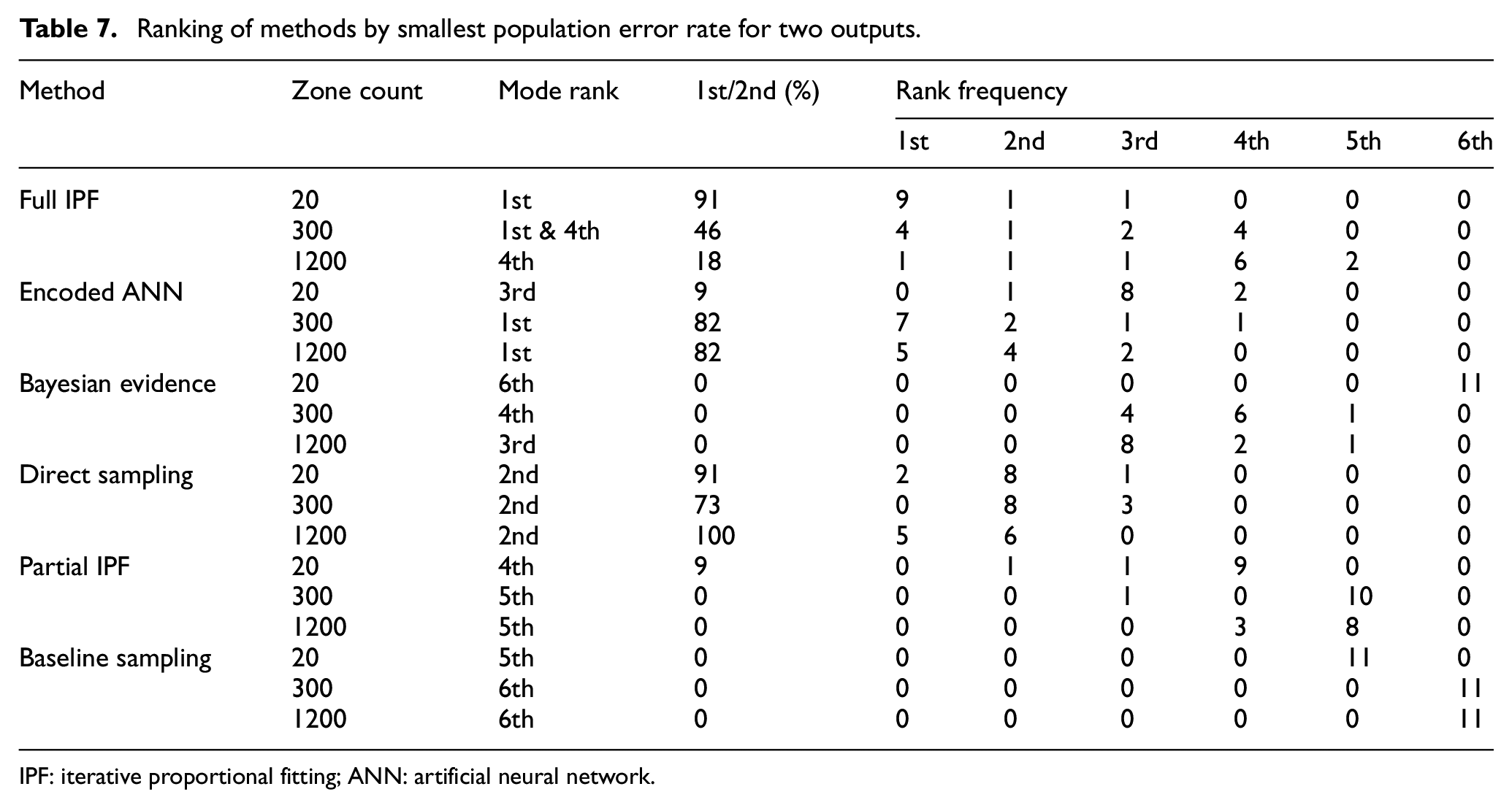
IPF: iterative proportional fitting; ANN: artificial neural network.

The full IPF technique declines to comparable performance with the partial IPF, which utilizes less of the control totals to recover the target population matrix and samples the uncontrolled variables. This would suggest that the full IPF struggles as more cell count frequencies approach one and becomes more reliant upon the stochastic element of TRS integerization to select individuals.

The partial IPF technique is only particularly effective in the dense zone count 20 scenario, indicating that other methods than IPF are more appropriate when zone contingency tables are available. The Bayesian evidence technique does not perform strongly and is exceeded by even the baseline sampling technique. Its relative performance improves as the population becomes sparser, but may be attributable to a decline in other techniques.

Increasing the decision space to three, see Figure 15, and four outputs, see Figure 16, provide a benefit to the full IPF technique in the densest scenarios of zone count 20 but is again not continued in the larger variable combinations for the observation space. There the encoded ANN can provide the lowest relative error rate followed by direct sampling. The gap between the full IPF and partial IPF narrows so that little difference is demonstrated between them, despite the full IPF having additional control total information. Both begin to track alongside the baseline sampling technique demonstrating a lack of effectiveness at these variable combinations and population sparsity.

Figure 15.

Population error rate across zone counts for three outputs (smaller is better).

Figure 16.

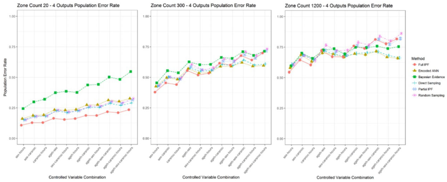
Population error rate across zone counts for four outputs (smaller is better).

Consider that the absolute error rate can be seen to quickly exceed 25% for all variable combinations when the population size is sparser than zone count 20. In some scenarios the techniques are producing error rates of greater than 50%, meaning that more than half of the populations have been misallocated.

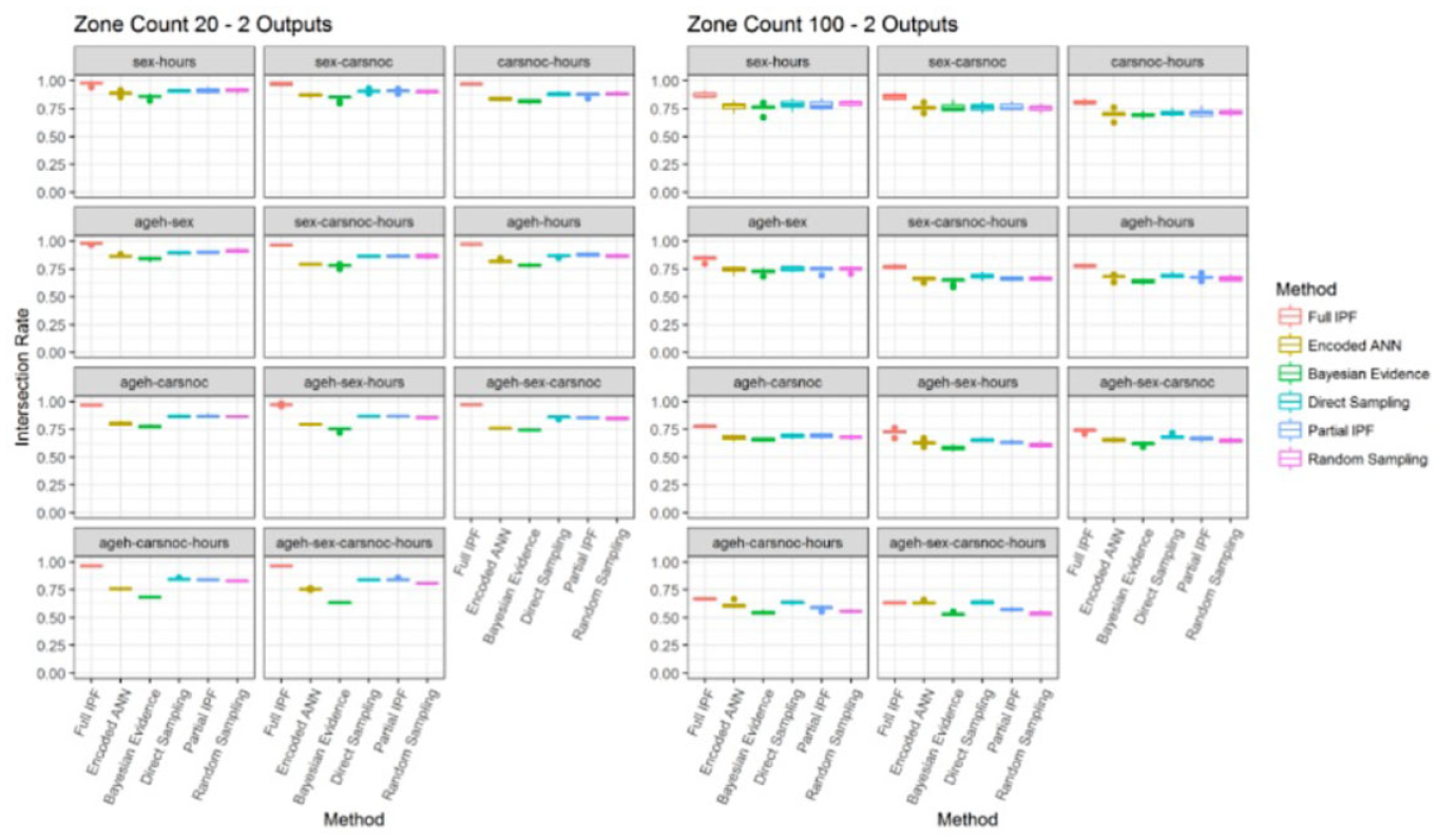
These errors could still occur with similar populations or be the result of incorrect archetypes being synthesized. Applying Jaccard similarity coefficient across the different population sizes for two outputs shows high levels of similarity in the densest zone count 20, as can be observed in Figure 17. The full IPF technique reports high levels across the variable combinations staying above 0.75 with comparable similarity for all other techniques, except Bayesian evidence.

Figure 17.

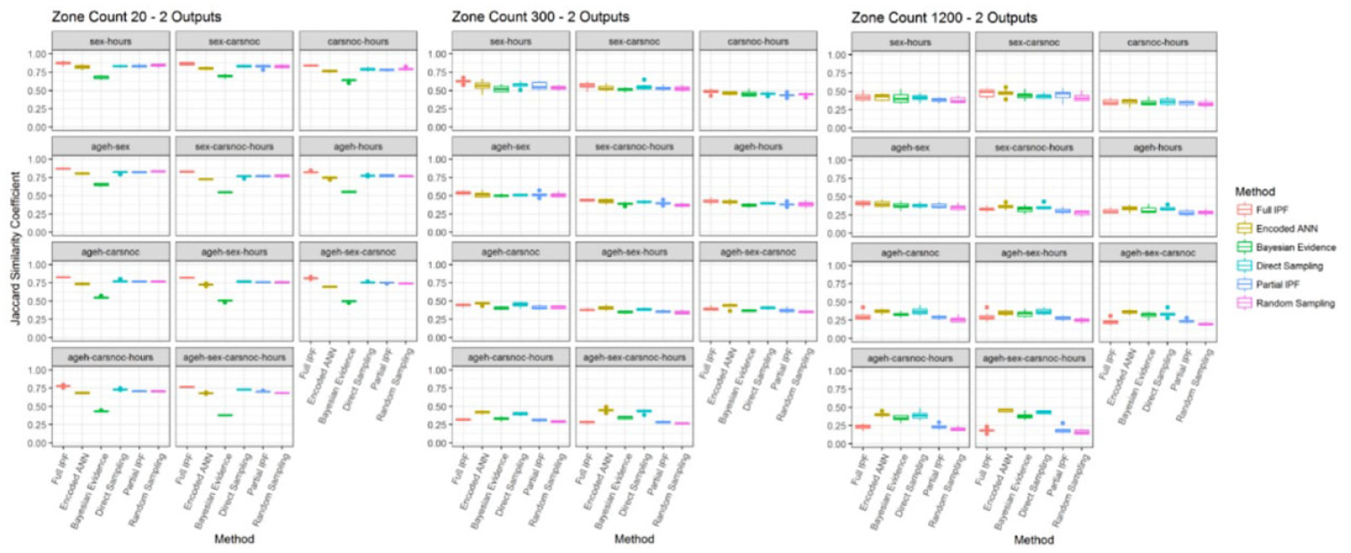
Jaccard similarity coefficient for two output variables across zone sizes (bigger is better).

Increasing the population sparsity in zone count 300 and 1200 leads to declining similarity across the techniques. In these sparser conditions, as the observation space is increased the encoded ANN and direct sampling techniques can keep higher levels of similarity compared with the other techniques. However, in absolute terms these techniques are still around the 50% region, meaning that a large proportion of archetypes from the actual population are not present or additional incorrect archetypes are being included.

When examining the harder scenarios by increasing the number of output variables a comparable situation emerges; see Figure 18. While the denser population of zone count 20 shows quite high levels of similarity, led by the full IPF technique, this declines distinctly in the other two zone sizes where all similarity levels are close or below 25%. This distinctly shows that these scenarios are not producing meaningful synthesized populations.

Figure 18.

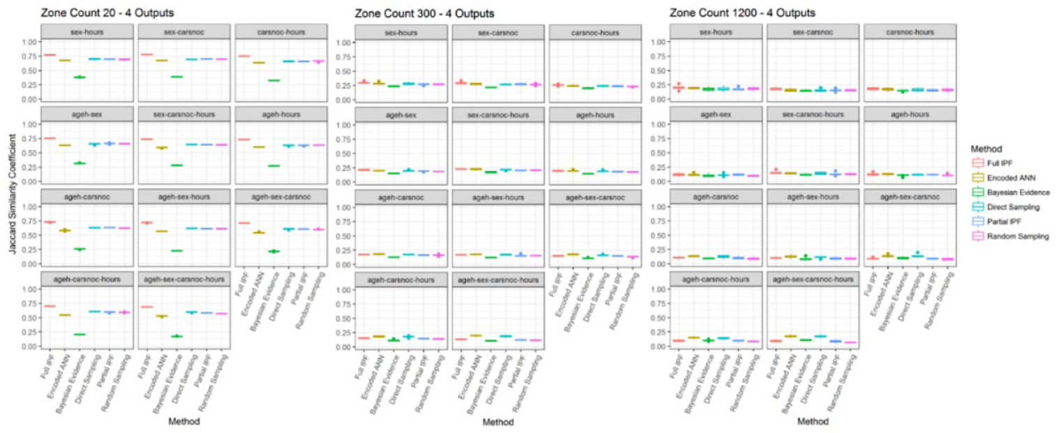
Jaccard similarity coefficient for four output variables across zone sizes (bigger is better).

Applying the additional metrics, the underlying cause for the decline in similarity can be examined. As can be noticed in Figure 19, the intersection rate across the zone sizes for four outputs in the zone count 20 the levels for each technique remain consistent. The encoded ANN technique shows a decline from 80.33% to 61.73%, while full IPF ranges from 97.55% to 94.38%. However, when the population becomes sparser the results for all techniques decline as variable combinations increase. In zone count 300 the full IPF technique now shows much less impressive values between 54.37% and 23.11%, while the encoded ANN achieves relatively better coverage in some variable combinations with values between 47.14% and 26.71%.

Figure 19.

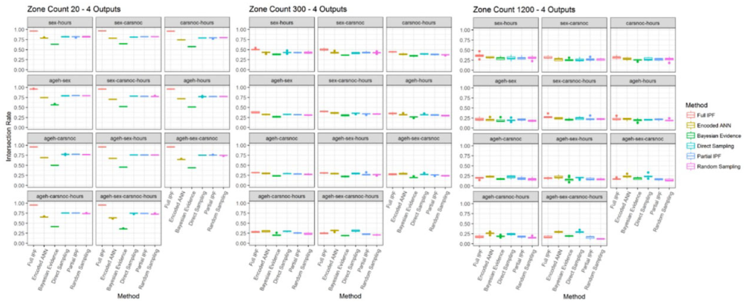
Intersection rate for four output variables across zone sizes (bigger is better).

Figure 20 shows that the decline in the inclusion of correct archetypes is matched by the increasing presence of incorrect archetypes as measured by the difference rate—predicted versus actual. In the zone count 20 scenario the level of incorrect archetypes remains between 15.51% and 29.11% for all techniques except Bayesian evidence. These levels rise dramatically to at least 50% for all techniques across all the variable combinations in the sparser scenarios and means that at least half of the archetypes present in the synthesized populations are incorrect. This result is regardless of the frequency of these archetypes occurring and reflects that they should not be present at all rather than being present in relative numbers, as indicated by the error rate measures.

Figure 20.

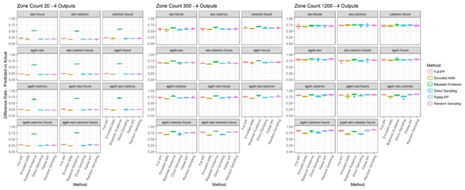
Difference rate—predicted versus actual for four output variables across zone sizes (smaller is better).

There is also a consistent pattern of the encoded ANN and direct sampling techniques having lower difference rates than the full IPF techniques. This means that while the full IPF technique includes more of the correct archetypes, it also includes more incorrect archetypes. The encoded ANN and direct sampling instead include a smaller set of archetypes, as seen in Figure 21, but those included are more likely to be correct.

Figure 21.

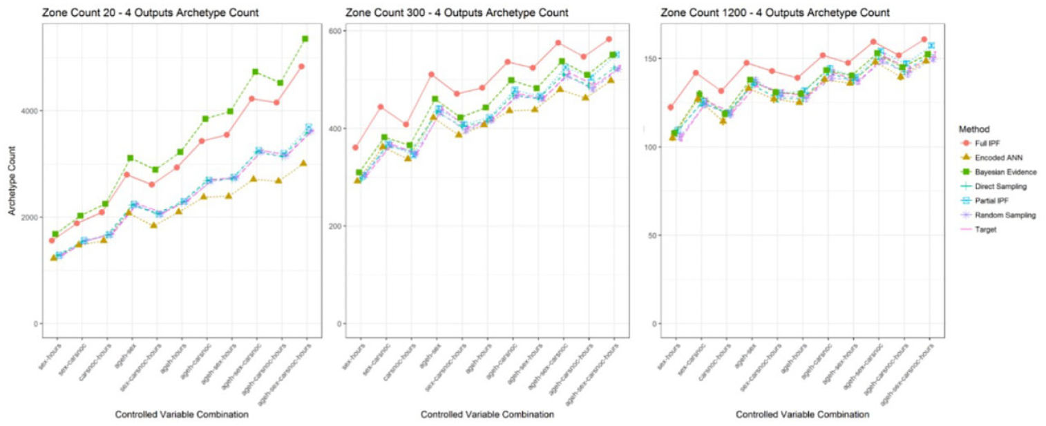
Number of archetypes in predicted population for four outputs across zone sizes.

A practical consideration is the time taken by each technique to perform the synthesize process, as recorded in Table 8. The experiments were performed using R version 3.3.1 with the latest package versions and using R Studio version 0.99.903 and run on a Windows 10 Pro x64 PC with an 8 core Intel i7-4820k processor, 16 GB RAM and 480GB Samsung EVO SSD drive. The encoded ANN differs from the other techniques in only needing to be trained once for each reference sample to a specific set of input and output variables and can then be applied to any target zone size as required. The other techniques are produced for the specific reference sample, input and output variables, and target zone. Therefore, after training the encoded ANN can produce a series of different zone populations very quickly.

Table 8.

Execution times for all techniques (seconds).

Outputs	Method	Min	Mean	SD	Max
2	Full IPF	0.05	0.41	0.55	3.13
	Encoded ANN	21.54	290.83	295.02	1004.25
	Bayesian Evidence	0.30	1.48	1.55	9.19
	Direct Sampling	0.06	1.20	1.39	6.11
	Partial IPF	0.09	1.23	1.33	5.00
	Baseline Sampling	0.00	0.00	0.01	0.02
3	Full IPF	0.14	5.56	8.96	46.09
	Encoded ANN	475.04	3736.57	2930.78	10,256.52
	Bayesian evidence	0.50	2.02	1.64	9.56
	Direct sampling	0.07	1.20	1.37	4.91
	Partial IPF	0.09	1.26	1.37	5.11
	Baseline sampling	0.00	0.00	0.01	0.03
4	Full IPF	1.01	12.05	14.34	59.38
	Encoded ANN	7212.53	31,223.84	18,709.51	66,368.92
	Bayesian Evidence	1.67	3.78	2.75	18.14
	Direct Sampling	0.08	1.32	1.49	5.76
	Partial IPF	0.08	1.37	1.46	5.68
	Baseline sampling	0.00	0.00	0.01	0.05

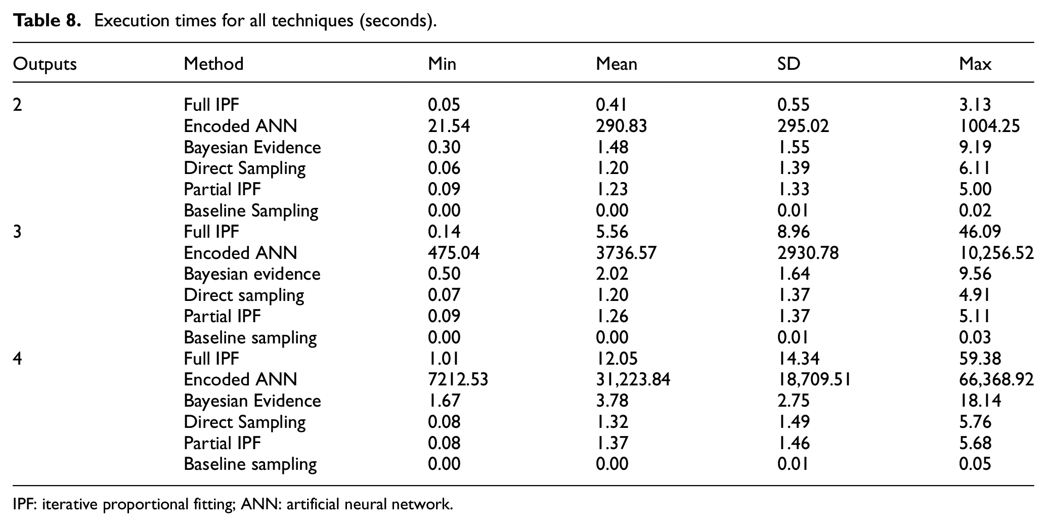
IPF: iterative proportional fitting; ANN: artificial neural network.

However, the encoded ANN takes considerably longer than the other techniques to produce a single zone population. The other techniques take from a few seconds and up to a minute in all scenarios. The encoded ANN ranges from 21 s to several hours with 18.44 h in the worst case. This running time could potentially be shortened by reducing the maximum number of iterations, which was set quite high in these experiments but will likely impact accuracy. Overall, this represents a disadvantage for the encoded ANN technique even though population synthesis is not generally a time critical activity.

We identified that the full IPF technique declines in relative effectiveness as the population becomes sparser. Although exhaustive variation of zone sizes has not been undertaken, this can be seen to occur between zone count 20, representing a 5% sample, and zone count 100, representing a 1% sample. As can be observed in Figure 22, in the two output scenario for these zone sizes, the full IPF declines as the variable combinations increase the observation space. A narrow difference at the largest variable combinations becomes much larger and occurs sooner once the population sparsity is changed from zone count 20 to zone count 100.

Figure 22.

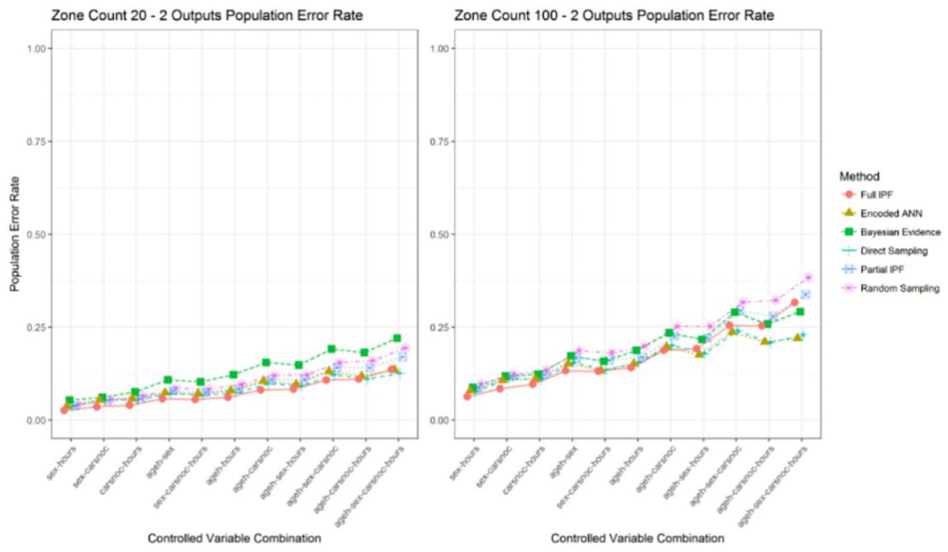
Population error rate across zone count 20 and 100 for two outputs (smaller is better).

Examination of the intersection rate in Figure 23 shows the very strong performance of full IPF declining down to the level of the other techniques. In the denser population the intersection rate ranged between 94% and 100%, but this is reduced to between 92% and 62%. Although still comparable to other techniques, the full IPF has also been shown to introduce more incorrect archetypes than the other techniques and demonstrated decline in performance.

Figure 23.

Intersection rate across zone count 20 and 100 for two outputs (bigger is better).

When the number of outputs is increased to four the full IPF demonstrated a good relative error rate in zone count 20, as can be observed in Figure 24. However, this declines again as the population sparsity is increased. It can again be observed as recorded in Figure 25, that the intersection rate ranges from 94% to 98% in zone count 20, but this declines into the range of 39% to 68% in zone count 100.

Figure 24.

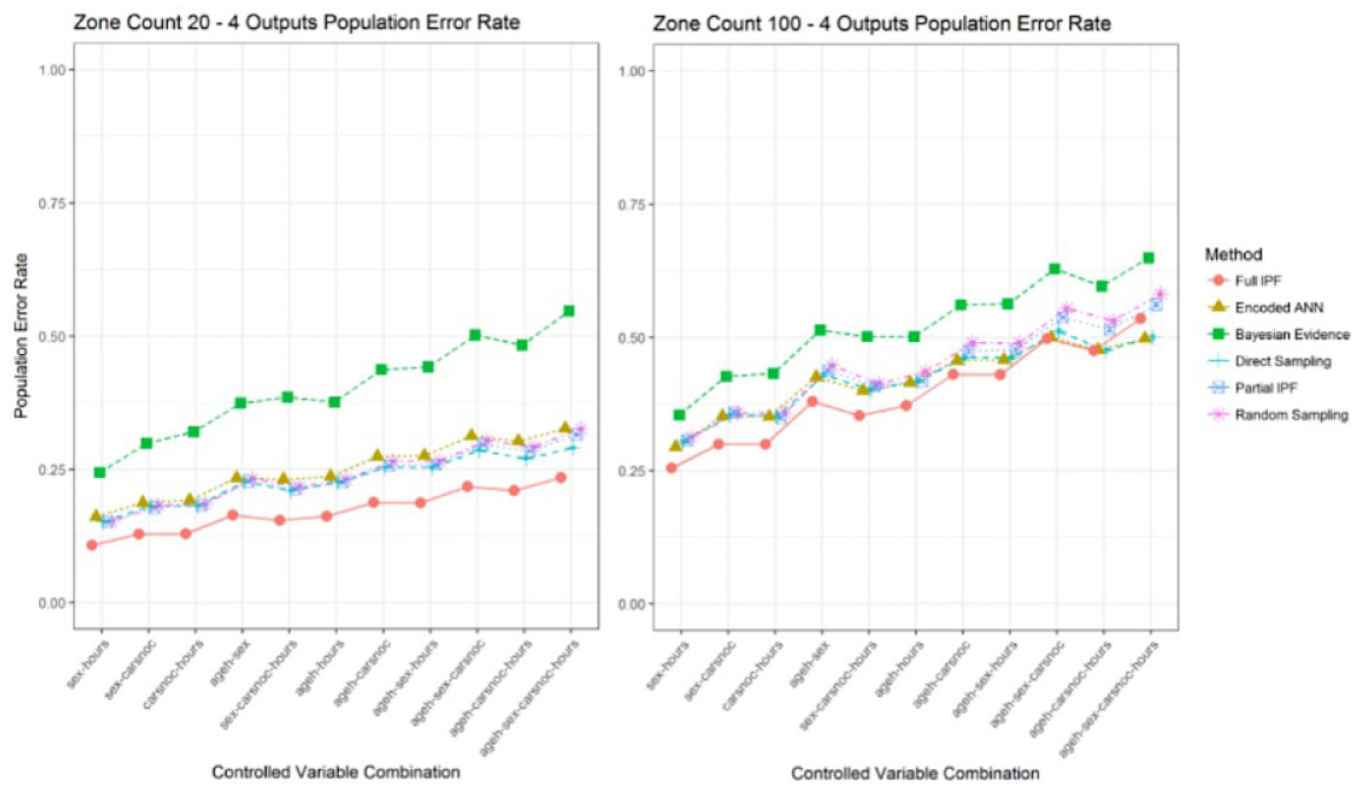
Population error rate across zone count 20 and 100 for four outputs (smaller is better).

Figure 25.

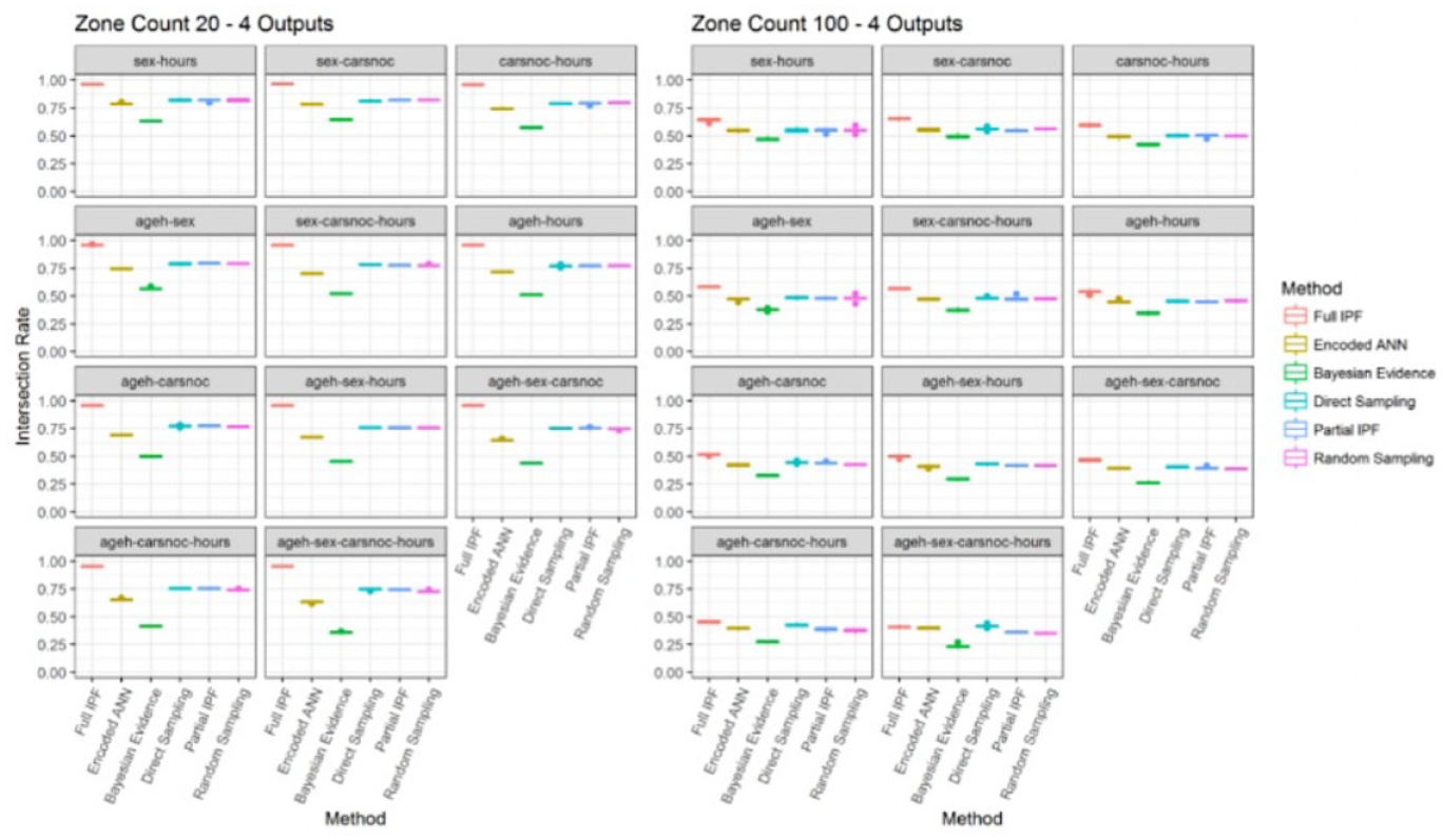
Intersection rate across zone count 20 and 100 for four outputs (bigger is better).

Once again, the advantage in intersection rate that full IPF exhibits at the densest population size of 5% sample size is lost in the change to 1% sample size. A more precise indication of the sample size trigger point and cause of this decline would require further investigation. Whether it is related to the sample size of the reference sample being 5% is unlikely and a more likely explanation is that greater proportions of single cases for each archetype are in the target zone population. This will mean that more of the population is synthesized through the stochastic step of the TRS integerization process rather than the deterministic step when values greater than one are present.

7. Conclusion

This research work proposed an ANN approach and simplified sampling approaches for population synthesis targeting the traffic simulation domain. We conducted a series of experiments to investigate the relevant error metrics and evaluate the performance of the developed synthesis approach. The findings of the research provide the following responses to the initial research questions:

RQ1: The proposed metric of Jaccard similarity coefficient has assisted in demonstrating the quality of the synthesized populations compared with the target populations by specifically showing the divergence in archetype coverage. The discussed error rate metrics show errors occurring through both coverage divergence and the distribution of archetypes. We performed further investigation using the related metrics of intersection rate and difference rate to establish the underlying behavior and cause of increasing error between techniques and scenarios, including the lower inclusion of the encoded ANN technique and the decline in the intersection rate for the full IPF technique.

There is also support that alternative goodness-of-fit error metrics to RMSE and SRMSE should be preferred. Our research established that the population error rate provides the most interpretable results in conjunction with the set theory metrics.

RQ2: The encoded ANN technique has performed consistently well against the alternative techniques of direct sampling, Bayesian evidence, partial IPF, and baseline sampling, which require the same or less information to perform. However, in scenarios with the largest population sizes and smallest number of input variable combinations the full IPF technique has shown to be more effective in terms of lower error and higher inclusion of correct archetypes. Encoded ANN has shown to be better at excluding incorrect archetypes compared with full IPF.

Overall, the results support the preference for IPF when full control totals are available but suggest caution when applied to sparse populations or more variables. The population quality in these scenarios is low and may not be of practical use. The main drawback of the encoded ANN technique is the slow training time, although models can be reused.

RQ3: The direct sampling technique demonstrates a consistency of performance across all the population sizes. It is second to the full IPF in the larger populations and marginally behind the encoded ANN in the smaller populations in terms of error rate and similarity. This result is possibly due to the large proportion of archetypes which have a single individual in the reference sample. The filtering of the controlled variables to a selection with a single choice for uncontrolled variables removes the element of randomness. It is a quick and simple technique to implement and execute, which gives it an advantage in practical scenarios where the full IPF cannot be used.

The use of baseline sampling has demonstrated that more complex techniques are justified but that in certain conditions the IPF methods can show performance that is only marginally improved.

RQ4: Does varying the population size in seeking smaller geographic area coverage influence the effectiveness of population synthesis techniques?

Our investigation revealed that the reduction in sample size does have an impact on the techniques and particularly affects the full IPF relative to the other techniques. The technique declines toward the partial IPF technique, which uses less information, and is only marginally improved on the baseline sampling technique when population sizes are small relative to the archetype diversity. Based on the obtained results, the use of the medium and smallest geographic areas or eight variables present very challenging scenarios for all the techniques with declines in the quality of populations produced.

The findings of the research suggest several areas for future work. The combining of multiple ANNs using a logistic regression mixture model approach would reduce the large number of categories in the response variable that could be affecting model accuracy. The approach could also be applied to the problem of multilevel fitting population synthesis. Further exploration is also needed for model tuning, such as weight decay and Bayesian Learning, or use of multiple hidden layers to allow fitting of both local and global features. We can also consider the treatment of datasets to reduce infrequent archetypes through dimensionality reduction techniques. A final area for further research can be investigating the correlation of population synthesis to the uncertainty associated with travel demand simulation; Zhang et. al used fuzzy logic theory to model uncertainty in the simulation of passenger behavior. ⁴⁸