Sage Journals: Discover world-class research

Abstract

Marine cranes are one of the most important industrial equipment in the maritime field. The base of a marine crane is dynamically moving as the motion of the ship’s six degrees of freedom that is affected by offshore environmental loads. There is a coupling between the crane and the ship, which means the crane operation and the ship motion affect each other. In this paper, co-simulation technology is employed to construct the virtual marine operation system which is composed of diverse Functional Mock-Up Units (FMUs) exported using the Functional Mock-Up Interface (FMI) standard and System Structure and Parameterization (SSP) standard to define the structure and parameters based on the co-simulation platform Vico. A path planning case for the Palfinger crane is implemented using the A* algorithm. The physical three-dimensional working space of the crane is discretized into a finite number of nodes in joint space. The cost is defined by the variable of the ship motion to optimize the marine operation. The obtained discrete nodes are smoothed to get the velocity of the actuators as control signals. Simulation of the crane operation is carried out in the virtual operating system following the planned path.

Keywords

Marine crane marine operation co-simulation path planning A*

1. Introduction

The crane plays an important role in the modern engineering field. It is installed in diverse scenarios mainly used for transporting objects. Marine cranes are also indispensable in the maritime field, and they are widely seen on ships and marine platforms. Today, the maritime industry is emphasizing more and more on the development and utilization of marine resources, which leads to high requirements and demands for marine operations. For example, the installation of offshore wind turbines regarding the development of offshore wind power,¹ and the exploration of subsea oil and gas resources.² Different from land-based cranes, the operations of marine cranes are facing more challenges in various aspects such as safety and efficiency due to the complex working conditions.³ Rough weathers induce intense external disturbances. Operations, especially heavy lifting, involve additional risks, not only posing threats to the working surroundings, for example, other onboard cargo, equipment, or working engineers but also producing a counteractive for ship motions itself. Therefore, marine operations are supposed to be conducted with safety, dependability, and operability in such a sense.

Today, digitalization and automation are increasingly being implemented to enhance efficiency and innovation in the marine industry. Modern ships are operating with many of their subsystems interacting with each other, whereas the marine crane operation system is also included with its subsystems. A virtual system can reduce the time and cost associated with research and development. The digital twin refers to a virtual representation of a physical system or object. It enables better design and optimizes the products, operations, and services achieved via real-time prediction, optimization, monitoring, controlling, and improved decision-making. Therefore, modeling and simulation are both important technologies. The past few decades have seen increasing developments in crane models and simulations from diverse applications and methods. For instance, three-dimensional models of container cranes subject to wind loads introducing Augmented Lagrangian based on the Lagrange method,⁴ the modeling of a forestry forwarder crane using Euler–Lagrange formulations to describe the equations of motion,⁵ the modeling of offshore crane hydraulic system using the bond-graph method,⁶ and many other modeling and developing research for crane compensation control containing winch hoisting system, payload system,⁷ etc. All of the findings are from the perspective of different domains involving mechanics, kinematics, multi-body dynamics, hydraulics, etc. That is because the crane is a typical multidisciplinary field product containing complex multi-domain systems. Researchers have tried to combine models of the multi-domain system within an integrated environment.⁸ However, the simulation in a homogeneous environment is confined to a large extent to the extension of software packages and the development of toolboxes. Compared to this, co-simulation enables each of the subsystems to be modeled by use of its specialized software tool.⁹ It combines the subsystems in a new way and characterizes distributed simulations, thereby lowering the computational load and improving the performance in heavy simulations. Co-simulation technology is emerging as a promising technique in complex marine system modeling. It enables better integration and cooperation of digitized virtual systems, being employed to develop advanced onboard support, such as risk assessment, behavior prediction, performance improvement, and control optimization.

In this paper, we use co-simulation technology to construct a virtual marine system based on the co-simulation platform Vico. The system is present in detail regarding three main constructions including the ship maneuvering, the crane operation, and the motion and force transfer. Based on the virtual system, a path planning strategy using A* algorithm with a four-dimensional grid map is implemented. The cost is defined by the variable of the ship motion to optimize the marine operation. The rest of the paper is organized as follows: section 2 presents the state of the art regarding the related fields. Section 3 provides a detailed introduction to the virtual marine operation system and section 4 illustrates the implementation of the planning algorithm. The specific case study is implemented in section 5; the simulation is carried out and the results are shown. Last, the conclusion and future work are discussed in section 6.

2. State of art

2.1. Co-simulation

In modern engineering, there are many technical issues within various systems, such as control systems, electric power systems, and aircraft motion systems. Most of the models of the system are described in the form of mathematical ordinary differential equations (ODE) and differential-algebraic equations (DAE).^10,11 In fact, the essence of engineering system simulation is to solve the initial value problem (IVP) of ODE and DAE. Complex multi-domain systems have the characteristics of multidisciplinary intersection, and also the manufacturing cycle of physical prototypes is long and costly. For this reason, the development of computer technology prompted a new tendency, that is, using co-simulation techniques to conduct the simulations and analysis of virtual prototypes regarding complex multi-domain systems.

Recent advances in co-simulation technologies have been significant starting in the automotive industry. The ITEA2 project MODELISAR first proposed Functional Mock-Up Interface (FMI), which is maintained and developed by Modelica Association.¹² It is a tool-independent standard that enables sub-model binary to be able to compatible with each other. This kind of shared, standardized interfaces (e.g., FMI) and model transformations on a shared format (e.g., XML) can achieve reuse and exchange of the models, which provides a better solution to maximize the efficiency of collaborating with research and development engineers from various disciplines and take advantage of single-discipline simulation software.⁹ The model for the implementation of FMI is called Functional Mock-Up Unit (FMU). It is an archive file in zip format with the extension .fmu. Normally, the zip file contains one XML file with the extension .xml describing the interface information, C or binary codes for one or more platforms, and some other optional document files. The FMI standard is closely aligned with the System Structure and Parameterization (SSP) standard¹³ which is a tool-independent standard to define complete systems consisting of one or more components (such as FMUs) including their parameterization. For now, there has been plenty of libraries and software tools created for supporting the FMI standard, which is a strong indication of its adoption in force. Some open-source co-simulation frameworks have been developed supporting both the FMI standard and the SSP standard, such as FMPy,¹⁴ libcosim,¹⁵ and OMSimulator.¹⁶ The maritime industry could also benefit from co-simulation technology,^17–19 which is also promoting digitalization and intelligence with the digital twin as the innovation.²⁰ An open platform can better facilitate collaboration within the maritime industry, where the models and data they contribute to each other are packaged as black boxes, ensuring that the intellectual property of all parties gets protected.²¹ Despite the advantages of co-simulation from different aspects, co-simulation also has its limitations and challenges. There is no guarantee that all sub-models of co-simulation will work perfectly together, and no general and easy-to-use solution is available. The efficiency of simulations is increased at the cost of loss of accuracy, and the performance also lacks a benchmark regarding model simplification. These issues also exist in a co-simulation.^22–26

2.2. Path planning

Path planning, also known as motion planning, or trajectory planning, is a class of computational problems, where a sequence of valid configurations is expected to be obtained to satisfy the motion for objects from the source to the destination. The essence of this class of problems is to solve equations with boundary constraints and seek optimal solutions. It is widely used in the modern engineering field, typically for robotics. Defining and constructing a countable state space for efficient search under certain criteria is a general solution for such problems.²¹ There are diverse contributed algorithms, which can date back to the 1970s, mainly the potential field method²⁷ and the elastic band method.²⁸ They may get stuck in local minimums of the potential field that prevent them from finding paths, or they may find non-optimal paths, which confines them within simple constrained problems. To cover complex constraints, sampling-based planning is proposed.^29,30 This method can be applicable to high-dimensional configuration spaces, but it takes more time and is usually exponential. They are complete in probability, which means that the probability to produce a solution is able to approach 1 as long as enough time is spent. Graph search algorithms are a branch of path planning search algorithms. The classic search algorithms are Dijkstra and A*. They are grid-based aiming to discretize a set of actions and build tree-like paths through grid points.^31,32 However, the number of grid points also grows exponentially when configuring the space, which makes them unable to configure paths in higher dimensional spaces. On the contrary, coarse discretization leads to an increase in the distance between grid points such that the path searched is not smooth enough as expected. In addition, there are also evolutionary algorithms that can be used for path planning applications. The Generic Algorithm is proposed based on Darwin’s evolution theory and is widely used for optimization problems. It is widely used in optimization problems because it can be applied to complex problems and can be processed with different parameters. A notable point is that the parameters are diverse and need to be selected properly for different problems so that the system can reach convergence. Other methods that can also deal with optimization problems expressed in terms of parameters are particle swarm optimization and machine learning.^33,34

The development of intelligence and automation has promoted a higher demand for improved safety and efficiency in the maritime industry. Intelligent and autonomous marine operations are also increasingly in place as a focus of the research. One of the most widespread applications of path planning is the optimization of the trajectory of marine vehicles.³⁵ As for offshore cranes, most of the studies are carried out following their modeling for compensating control where the path or trajectory planning is included as part of it. For example, He et al.³⁶ converted the problem of the trajectory planning problems of the offshore crane into the planning problems for flat outputs using the flatness theory, then used a bisection-based method to solve the formulated time optimization problem and the optimal transportation time, together with the time optimal reference trajectories obtained. Lu et al.³⁷ proposed an online trajectory planning method regarding three-dimensional offshore boom cranes including boom luffing/rotating and rope hoisting motions. The introduced extra coupling terms into the input signals enable the original trajectories continuously make online adjustments. The comparative experiments demonstrate the robustness by inducing system uncertainty, external disturbances, etc.

3. Co-simulation framework

In this paper, the co-simulation framework Vico is employed to conduct the virtual marine operation system simulation. It is a novel high-level co-simulation framework, which is founded on a software architecture based on the entity component system (ECS) architecture.³⁸ Vico focuses on co-simulation and supports both the FMI standard and the SSP standard. The virtual marine operation system consists of two main subsystems separately—the ship maneuvering system and the crane operation system.

In the ship maneuvering system, there are in total 12 different models described by 9 different FMUs as shown in Figure 1. In particular, the Vessel Model was developed by SINTEF Ocean in the SimVal project,³⁹ which is in six degrees of freedom (6-DoF) with waves and solves the equations of motion containing the vessel’s restoring force, mass, resistance, and some other hydrodynamics information. It is implemented according to the unified non-linear model subjected to waves, wind, and currents from Fossen.⁴⁰ Three thrusters including a port-side azimuth thruster Azimuth0, a starboard-side azimuth thruster Azimuth1, and a tunnel thruster Tunnel Thruster produce forces in the directions of heave, surge, and sway. Each thruster is equipped with its own actuator where the power is provided by two equally large gensets in Power Plant. The forces for the three thrusters are different regarding different maneuvering. They are generated and allocated by the Allocator. The Observer computes the movement direction and the speed to get the position difference with time then shares the data with the Allocator. Waypoint Provider can generate the waypoints by providing input variables, which can be a fixed point as a station-keeping mode or a trajectory with multiple inputs. The DP Controller conducts the dynamic positioning, which can make sure the ship can stop at a relatively ideal fixed location in the world frame according to Waypoint Provider.

Figure 1.

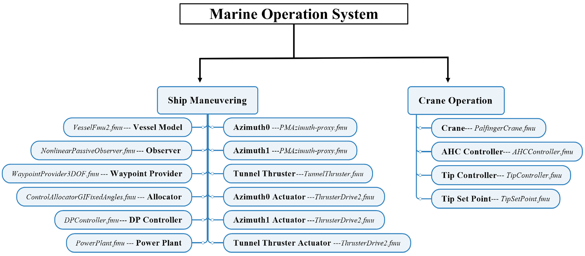
The construction of the virtual marine operation system in terms of FMU.

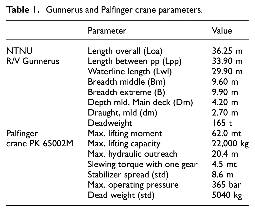
The crane model is developed based on the Palfinger crane installed on NTNU’s research vessel R/V Gunnerus, which is a kind of knuckle boom crane with four joint DoF as shown in Figure 2. The slewing motor can conduct the base rotation operation. The boom cylinder and the jib cylinder can change the second and the third joint angles to perform the luffing and lifting operation cooperated. The outer boom can extend to reach a wider field. Some main parameters of the Gunnerus and the Palfinger crane are given in Table 1. In the virtual marine operation system, the interfaces of four joint DoF are defined, which enable the crane can be operated from the joint space while the tip position can be calculated through forward kinematics. Meantime, it is also available to set the tip position to control the joints with inverse kinematics. The crane is also equipped with two compensation controllers; one is to compensate the payload in the heave direction by controlling the winch system and the other is to compensate the tip end also in the heave direction by inverse kinematics. Some detailed interface connection regarding compensation is shown in Figure 3.

Figure 2.

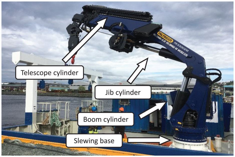
Palfinger crane installed on the R/V Gunnerus.

Table 1.

Gunnerus and Palfinger crane parameters.

	Parameter	Value
NTNU R/V Gunnerus	Length overall (Loa)	36.25 m
	Length between pp (Lpp)	33.90 m
	Waterline length (Lwl)	29.90 m
	Breadth middle (Bm)	9.60 m
	Breadth extreme (B)	9.90 m
	Depth mld. Main deck (Dm)	4.20 m
	Draught, mld (dm)	2.70 m
	Deadweight	165 t
Palfinger crane PK 65002M	Max. lifting moment	62.0 mt
	Max. lifting capacity	22,000 kg
	Max. hydraulic outreach	20.4 m
	Slewing torque with one gear	4.5 mt
	Stabilizer spread (std)	8.6 m
	Max. operating pressure	365 bar
	Dead weight (std)	5040 kg

Figure 3.

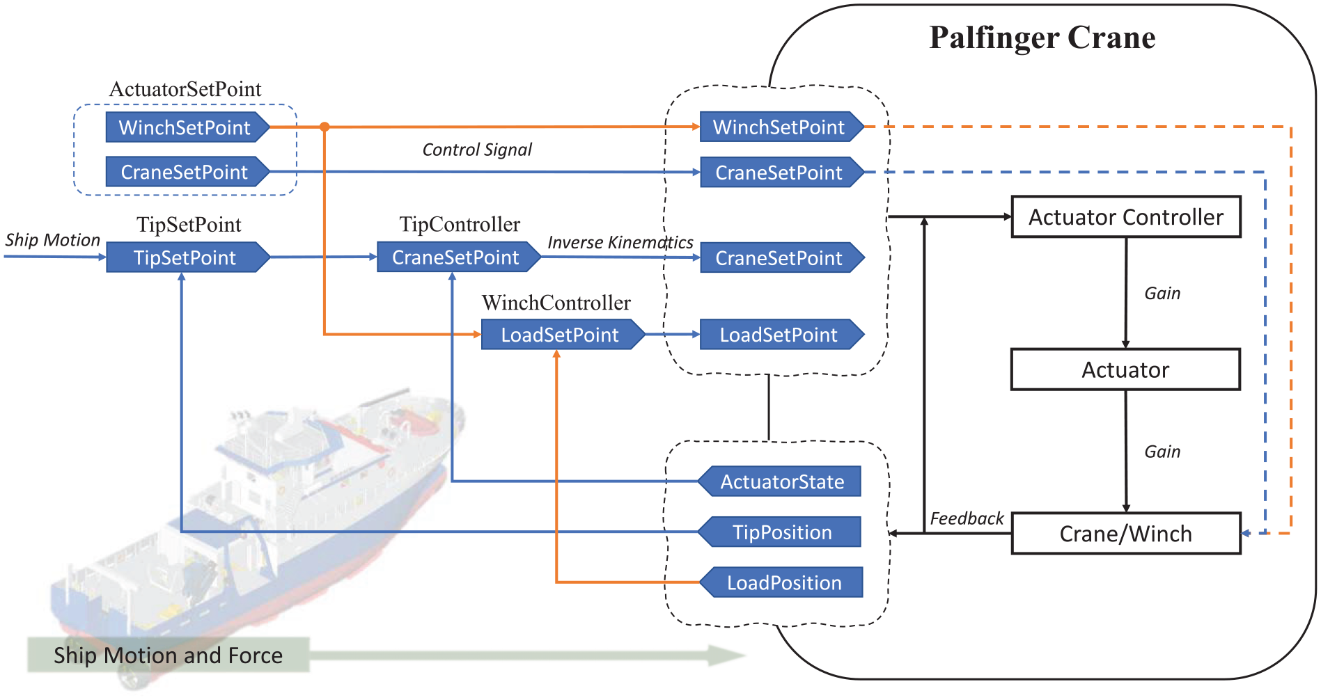
Interface connections among sub-models for crane operations.

During crane operation especially heavy lifting operation, it is easy to see that the dynamic inertia from the payload will lead to coupling issues between the ship and the crane, which is not seen as a negligible factor. Here, the forces from the crane and the payload are treated approximately as external forces attacking variant points of the ship hull. Figure 4 shows the detailed motion and forces exchange between the vessel and the crane. The crane base has the same motion as the ship hull with the motion in six DoF. The crane position is able to be modified via interfaces of the points of attack in three axes according to the configurations of different vessels. The connection between the payload and the crane is processed as a flexible cable.

Figure 4.

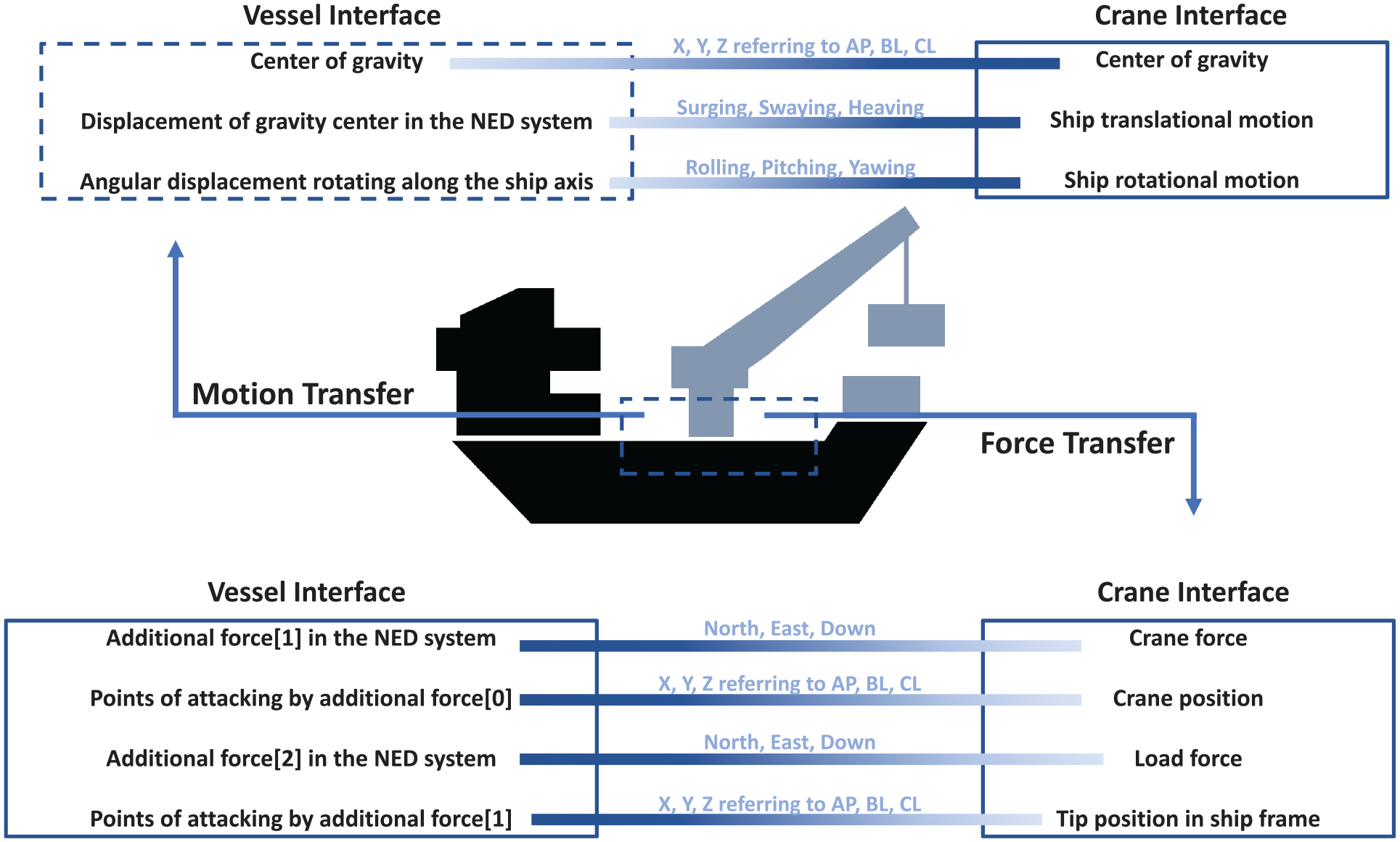
Interface connection of motion and force transfer between the vessel and the crane.

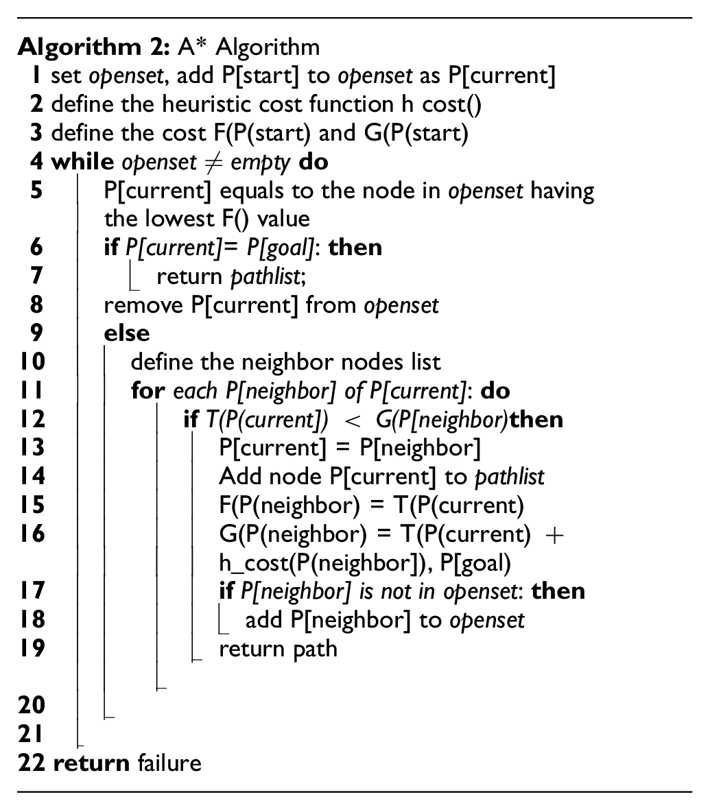
4. A* algorithm implementation

A* is a graph traversal and path search algorithm employed in many areas of computer science to achieve completeness, optimality, and optimal efficiency.⁴¹ It is proposed to get the path from the start point to the goal point with the minimum cost. It is developed based on the Dijkstra’s algorithm conducting the offline path planning with a grid map. Different from Dijkstra, it introduces a heuristic cost to estimate the cost from the current node to the goal node speeding up the searching process.⁴² While maintaining a priority queue of nodes to be explored, the algorithm starts by extending the node with the lowest estimated cost to the goal. If a better path is found, the cost of the previously visited node is then updated. It terminates when the goal is reached or when all reachable nodes have been explored. As described in Equation (1), where the final cost g(n) is the sum of the current cost f(n) and the heuristic cost h(n):

g (n) = f (n) + h (n)

(1)

In this paper, the A* algorithm is used to conduct the path planning for the crane tip. The tip moves in a physical three-dimensional space. The working space can be seen as a three-dimensional grid map in the coordinate of the ship frame by splitting each axis into certain lengths. In other words, instead of searching for the shortest path in each iteration, here the cost of the three-dimensional grid node calculation is present in a pre-known way as a dataset; instead, each node represents the cost used to evaluate the expected minimum cost in the marine operation system where a defined function for desired optimal performance is employed to evaluate the cost. Therefore, once we know the start and goal nodes of the path, the first cost value and the last cost value on the planned path are already calculated. To get the optimal performance of the crane operation affected by the ship motion subjected to the offshore condition, here the ship rolling motion response is taken as the cost evaluation variable. As shown in Figure 5, there presents an example of ship rolling motion response subjected to environmental conditions. Since the wave model follows the JONSWAP spectral distribution,⁴³ the motion of the ship is not periodical, and the maximum and minimum values of rolling during the process are used to calculate the amplitude of the rolling motion as shown in Equation (2).

Figure 5.

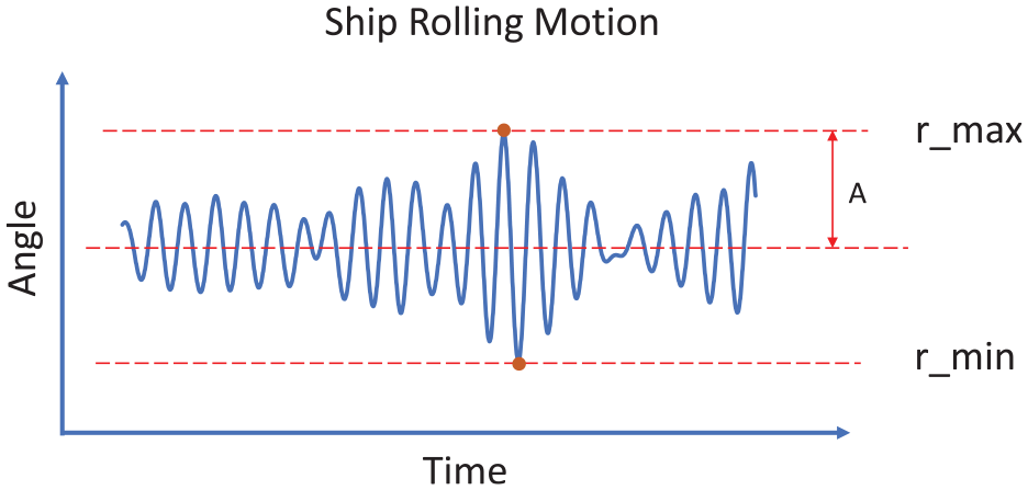
Ship rolling motion subjected to the environmental loads.

Thus, according to the above equation, the cost f(current) is the sum of the costs of all searched nodes on the path, and the cost g(current) is the estimated cost from the start node to the goal node via the current point. Since the cost of the desired path is evaluated by a variable during the marine operation, the estimated cost from the current node to the goal node can no longer be applicable like the norm value during the shortest path searching. The temporary cost t(current) equals the sum of the cost f(current) and the cost at the neighbor node cost(neighbor):

A = (r_\max - r_\min) / 2

(2)

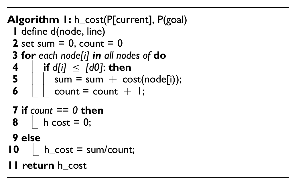
For the heuristic cost, we have a special definition as shown in Algorithm 1 and the sketch is shown in Figure 6. Simply, the spatial line can be obtained using two known nodes—the current node and the goal node. For each node in the spatial grid map, the distance between the node of the obtained line within a proper value will be counted. The average value calculated by dividing the counted number using the sum of the cost of counted nodes is regarded as the heuristic cost. In this way, the pseudo-code of a complete A* algorithm applying to the path planning for the marine crane can be written as shown in Algorithm 2.

Figure 6.

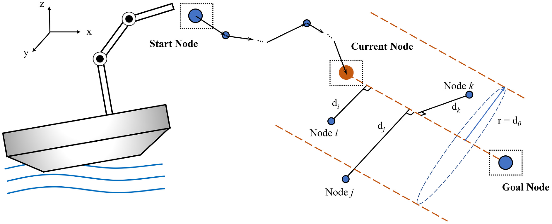
The illustration of the heuristic cost.

Algorithm 1: h_cost(P[current], P(goal)

1 define d(node, line)2 set sum = 0, count = 03 foreach node[i] in all nodes of do4 ifd[i] ≤ [d0]: then5 sum = sum + cost(node[i));6 count = count + 1;7 ifcount == 0 then8 h cost = 0;9 else10 h_cost = sum/count;11 return h_cost

Algorithm 2: A* Algorithm

1 set openset, add P[start] to openset as P[current]2 define the heuristic cost function h cost()3 define the cost F(P(start) and G(P(start)4 while

openset \neq empty

do5 P[current] equals to the node in openset having the lowest F() value6 ifP[current]= P[goal]: then7 return pathlist;8 remove P[current] from openset9 else10 define the neighbor nodes list11 foreach P[neighbor] of P[current]: do12 ifT(P(current]) < G(P[neighbor) then13 P[current] = P[neighbor]14 Add node P[current] to pathlist15 F(P(neighbor) = T(P(current)16 G(P(neighbor) = T(P(current) + h_cost(P(neighbor]), P[goal)17 ifP[neighbor] is not in openset: then18 add P[neighbor] to openset19 return path 20 21 22 return failure

5. Case study

In this section, a Palfinger crane path planning case is implemented based on the virtual marine operation system. Figure 7 explains the working flow using A* algorithm. First, the working space of the crane is sketched according to the crane information to obtain the grid map in three-dimensional space for the A* algorithm. According to the description of the A* algorithm in the previous section, each node in the grid map corresponds to a cost that is obtained from the simulation data in the corresponding cases with diverse crane orientations from the co-simulation platform. This means that the demanded crane operation described by a dynamic process is partitioned into a large number of finite static processes, and the cost of each static process is represented by the desired optimal variable values generated by the crane. As the rolling motion of a ship is dominating, and the cranes usually work from the sides of the ship, here we take the ship rolling motion amplitude as the cost value. Hence, so long as we determine the start and goal positions, the A* algorithm can search for the optimal solution to reach the goal in accordance with the cost of each node, which is the desired path with the expected optimal operation process. Since the path is composed of many nodes, the full path is not smooth enough with many folded connections. Considering the operation of the crane in the joint space, the discrete nodes obtained are smoothed to obtain the displacement and velocity curves for the joint control, which can be integrated into the actuator controller to operate the virtual marine operation to verify the final path.

Figure 7.

The crane actuating cylinders.

5.1. Data generating

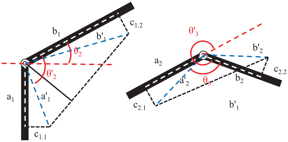
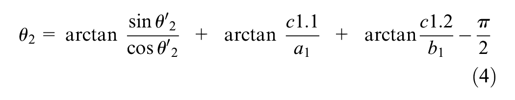
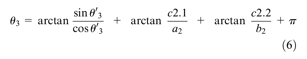
As shown in Figure 3, the operation of the base slewing is limited considering that the wheelhouse is a large obstacle as an unreachable area. Other restrictions on the operation of the rest joints are subject to the actual situation which are not considered here. From the perspective of forward kinematics, the crane’s physical working space can also be regarded as its different combinations of values in the four DoF in joint space. Therefore, the grid map for the working space can be generated by splitting the operation space of the four joint DoF. It is particularly noted that the second and third joint DoF of the Palfinger crane are the rotating angles of the boom and jib, which are controlled by the extension and shortening of the corresponding hydraulic cylinders in the hydraulic system of the crane. According to the mechanical model shown in Figure 8, the relationship between the joint angle and the cylinder length is given in Equations (3)–(6):

L_{1} = \sqrt{{a_{1}^{'}}^{2} + {b_{1}^{'}}^{2} - 2 {a'}_{1} {b'}_{1} \cos ({θ'}_{2})}

(3)

θ_{2} = \arctan \frac{\sin {θ'}_{2}}{\cos {θ'}_{2}} + \arctan \frac{c 1.1}{a_{1}} + \arctan \frac{c 1.2}{b_{1}} - \frac{π}{2}

(4)

L_{2} = \sqrt{{a_{2}^{'}}^{2} + {b_{2}^{'}}^{2} - 2 {a'}_{2} {b'}_{2} \cos ({θ'}_{3})}

(5)

θ_{3} = \arctan \frac{\sin {θ'}_{3}}{\cos {θ'}_{3}} + \arctan \frac{c 2.1}{a_{2}} + \arctan \frac{c 2.2}{b_{2}} + π

(6)

Figure 8.

The workflow for A* planning.

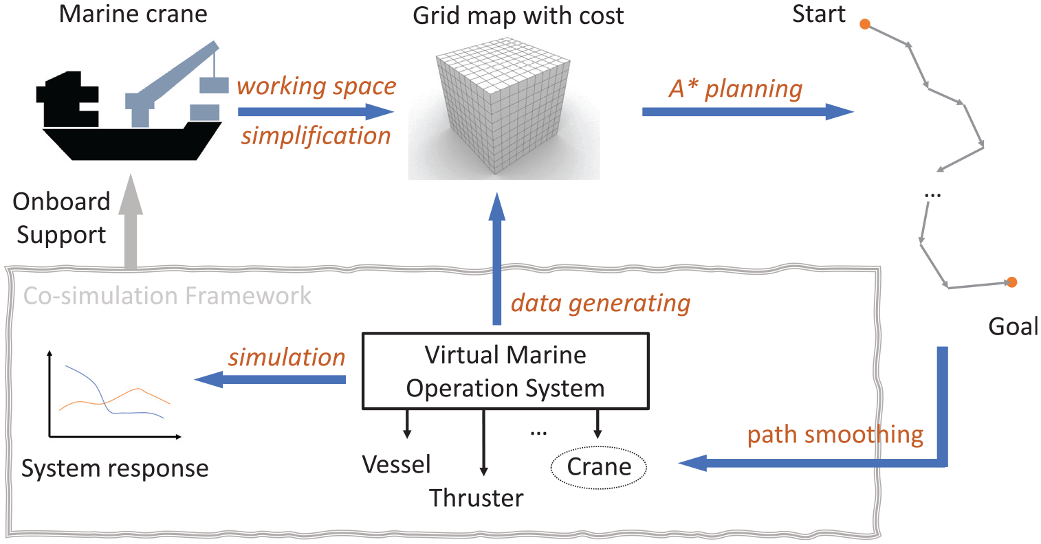
Thus, the operable interval of the four joint DoF is that slewing angle ranges from −15° to −315° with 6° as a node, the boom cylinder length ranges from 1.1 to 1.7 m with 0.2 m as a node, the jib cylinder length ranges from 1.2 to 1.8 m with 0.2 m as a node, the outer boom extension ranges from 1.5 to 11.5 m with 2 m as a node. It can be seen that the length for both the boom cylinder and the jib cylinder has only four different nodes because most of the time the lifting and dropping operations are conducted by winch. Of course, in case of demand, the grid map can be split finer, as this is not the focus of this paper, it is not discussed here. In this way, the crane’s working space in the virtual marine operating system becomes a 51 × 4 × 4 × 6 grid map in four-dimensional space from the view of the joint space, which corresponds to the same number of tip positions in physical three-dimensional space, and also the same number of crane orientations. To set a dataset, the environmental loads are configured as a slight condition with 0.5-m wave height, 10-s peak period, 0.1-m/s current velocity, and 1.0-m/s wind velocity. All the loads’ directions are set from 90°, which will generate the most torque on the ship and produce the most impact on the ship rolling motion. The DP controller is activated at 50 s from the start of the simulation, and the first 50 s of data are not taken into present due to the scenario generation, which explains the blank at the first 50s in Figure 12 and Figure 13. Following this way, a grid map in 3D space is obtained where all the nodes are cost-evaluated as the scatter plot shown in Figure 9. The darker the color, the greater the cost; and vice versa. The positive Y-axis direction is the ship’s heading side, and the positive X-axis direction is the starboard side. The blank area without nodes is considered the limited area due to the wheelhouse.

Figure 9.

Scatter plot for crane working space.

5.2. Results and discussion

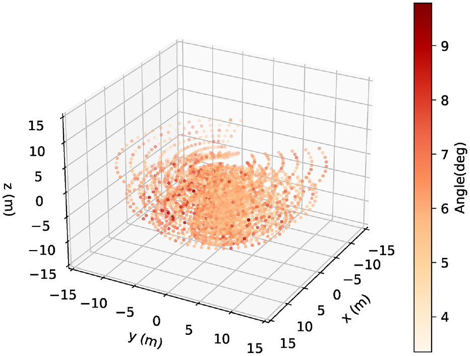
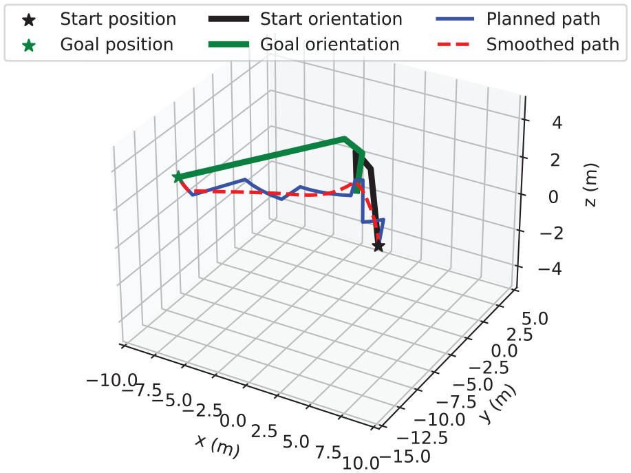
The crane operation is simulated with the start position (2.97, −2.14, −1.75) m and the goal position (−8.83, −9.68, 2.20) m in the ship frame. According to inverse kinematics, the joint angles can be obtained and matched to the nearby nodes in the grid map, so that the searching process can be carried out in the joint space where each time only one joint DoF changes to its neighboring nodes. The planning result is shown in Figure 10. The green manipulator is the start orientation of the crane and the black one is the goal orientation. The blue fold path is the planned path by A* algorithm. It can be seen that the path is not a smooth curve as it is just connected by the finite nodes directly from the grid map. To enable the operation more smoothly, the displacements of the joint angles are processed to the polynomials during its operation in Figure 11, so the final smoothed path is shown as the red dash line in Figure 10. In this way, the velocity curves can be also obtained to better control the actuators of the crane as shown in Figure 12. The operation starts at the 200 and finishes at the 410 s. Figure 13 presents the simulation results. The stepsize was chosen so that it satisfies the application’s accuracy constraints and computational time available. There is an offset between the center of the ship gravity and the crane frame, which explains the coordinate difference in tip position. The ship rolling motion increases during the crane operation and gradually decreases after the operation. It can be seen that at the time with the crane system is mainly excited by the ship rolling motion, the movement of the crane tip during its operation appears in the z-axis direction with large periodic oscillations, which also confirms the impact of rolling on the tip in the ship’s heave direction.

Figure 10.

The planned path using A* algorithm.

Figure 11.

Displacement and velocity of crane actuators.

Figure 12.

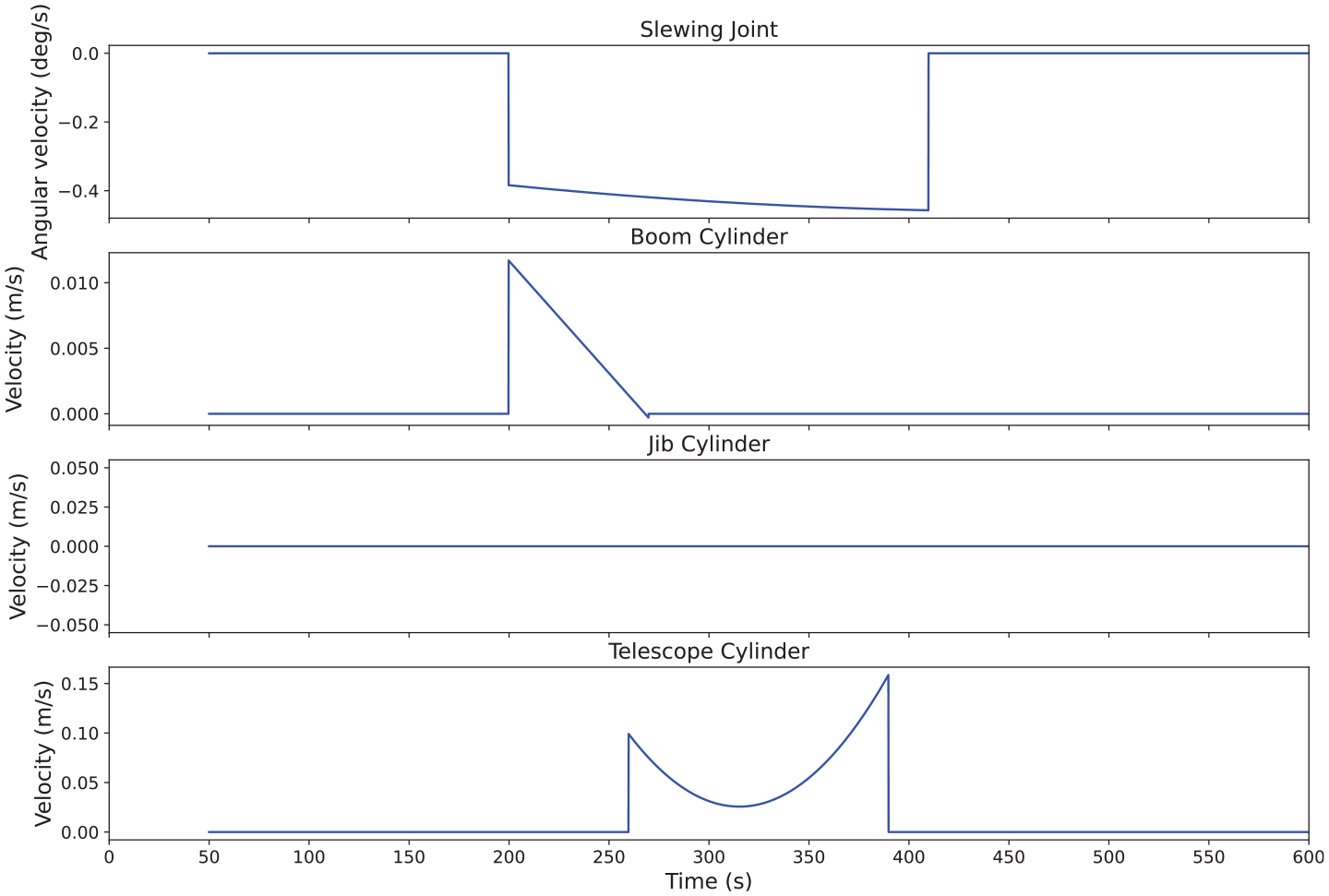
Control signals of the actuators.

Figure 13.

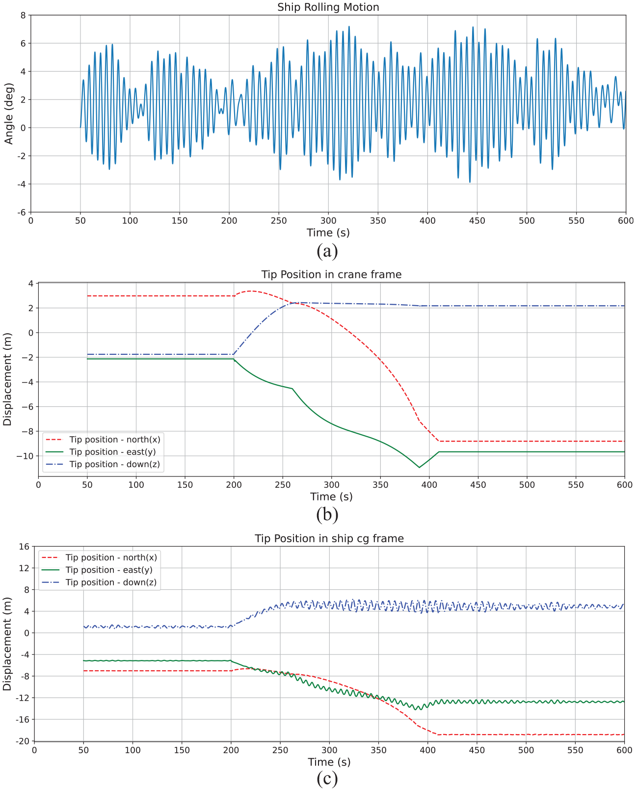
System response subjected to environmental loads.

From the planning view, the A* algorithm is regarded as an optimal solution. For the path planning of the marine crane, this paper uses a co-simulation platform to generate cost data to process the dynamic process at the cost of a static pose. This processing method also has the hidden premise that the operation process is performed at a very slow speed. This means that operational efficiency is also invisibly added to the cost function. The cost function can be designed according to different requirements, and the path produced by different cost functions will be different. A star algorithm to evaluate marine operations in this paper where the cost function is specially defined is not the optimal solution due to the fact that A* is not very well balanced to deal with all aspects of the dynamic process of crane path planning. It is only about the indicator that we focus and also can be defined as others. Therefore, the paper is more about demonstrating the contribution of the feasibility to develop marine onboard support application based on the virtual marine operation system using the co-simulation approach. The crane path planning is also an independent topic worthy of further study.

6. Conclusion

In this paper, we presented a virtual marine operation system using co-simulation technology based on the co-simulation platform Vico. The co-simulation framework can better handle multi-domain systems than the homogeneous simulation environment. This kind of parallel computation using multiple processes by different solvers improves the simulation efficiency. Based on the virtual system, we used the A* algorithm to conduct the path planning for the tip of the marine crane. The dynamic operation process is discretized into a finite number of statistic nodes with cost defined in a special way, which consist of a four-dimensional grip map. The ship rolling motion amplitude is considered as the evaluation parameter to optimize the operation regarding the coupling between the ship and the crane. The co-simulation technology of the marine operation framework still needs to be verified with real marine data to discuss stability and accuracy. The results provide the feasibility to conduct the application development of the marine operation onboard support based on the virtual marine operation system using co-simulation approach. The planning does not consider the large obstacles and limited working space other than the wheelhouse, which is one of the studies of path planning. As future work, co-simulation can be employed as the platform to optimize the algorithm for marine crane path planning. The dynamic cost is also considered as a better evaluation strategy to guarantee the optimal operation process between each node. Further simulations and research are to be carried out considering verification of the validation. As well, the compensation of the ship motion and the payload anti-swing issue are also one of the key points for crane operation.

Footnotes

Funding

The author Zizheng Liu would like to thank the sponsor ship of China Scholarship Council for funding his research at Norwegian University of Science and Technology.

ORCID iD

Zizheng Liu

Author biographies

Zizheng Liu is currently a PhD candidate at the Department of Ocean Operations and Civil Engineering, Faculty of Engineering, Norwegian University of Science and Technology.

Yingguang Chu is currently an Assistant Professor at the Department of Mechanical and Electrical Engineering, Faculty of Engineering, University of Southern Denmark.

Guoyuan Li is currently a Professor of ship intelligence at the Department of Ocean Operations and Civil Engineering, Norwegian University of Science and Technology.

Hans Petter Hildre is currently a Professor and Head of Department, Department of Ocean Operations and Civil Engineering, Norwegian University of Science and Technology.

Houxiang Zhang is currently a Full Professor at the Department of Ocean Operations and Civil Engineering, Faculty of Engineering, Norwegian University of Science and Technology. He was elected as a member of the Norwegian Academy of Technological Sciences in 2019.

References

Gao

Moan

, et al. Analysis of lifting operation of a monopile for an offshore wind turbine considering vessel shielding effects. Marine Struct 2014; 39: 287–314.

How

BVE

Choo

. Control of coupled vessel, crane, cable, and payload dynamics for subsea installation operations. IEEE Trans Control Syst Tech 2010; 19: 208–220.

Acero

Gao

, et al. Methodology for assessment of the operational limits and operability of marine operations. Ocean Eng 2016; 125: 308–327.

Arena

Casalotti

Lacarbonara

, et al. Dynamics of container cranes: three-dimensional modeling, full-scale experiments, and identification. Int J Mech Sci 2015; 93: 8–21.

La Hera

Morales

. Modeling dynamics of an electro-hydraulic servo actuated manipulator: a case study of a forestry forwarder crane. In: World Automation Congress, Puerto Vallarta, Mexico, 24–28 June 2012, pp. 1–6. New York: IEEE.

Chu

Æsøy

Zhang

, et al. Modelling and simulation of an offshore hydraulic crane, 2014, https://www.researchgate.net/publication/269227002_Modelling_And_Simulation_Of_An_Offshore_Hydraulic_Crane

Qian

Tong

Lee

. Fuzzy-logic-based control of payloads subjected to double-pendulum motion in overhead cranes. Autom Construct 2016; 65: 133–143.

Bak

Hansen

. Model based design optimization of operational reliability in offshore boom cranes. Int J Fluid Power 2013; 14: 53–65.

Gomes

Thule

Broman

, et al. Co-simulation: a survey. ACM Comput Surv 2018; 51: 1–33.

10.

De Jalon

Bayo

. Kinematic and dynamic simulation of multibody systems: the real-time challenge. New York: Springer, 2012.

11.

Bauchau

. Flexible multibody dynamics. vol 176. New York: Springer.

12.

Modelisar-Association. Functional mock-up interface, 2014, https://www.fmi-standard.org (accessed 16 February 2023).

13.

Köhler

Heinkel

Mai

, et al. Modelica-association-project “system structure and parameterization”–early insights. In: The First Japanese modelica conferences, Tokyo, Japan, 23–24 May 2016. Linköping: Linköping University Electronic Press.

14.

Catia-Systems. FMPy, 2020, https://github.com/CATIA-Systems/FMPy (accessed 16 February 2023).

15.

Open-Simulation-Platform. libcosim, 2020, https://github.com/open-simulation-platform/libcosim, 2020 (accessed 16 February 2023).

16.

Ochel

Braun

Thiele

, et al. Omsimulator–integrated FMI and TLM-based co-simulation with composite model editing and SSP. In: Proceedings of the 13th International Modelica Conference, Regensburg, 4–6 March 2019. Linköping: Linköping University Electronic Press.

17.

Chu

Pedersen

Zhang

. Virtual prototyping for maritime winch design and operations based on functional mock-up interface co-simulation. Ships Offshore Struct 2019; 14: 261–269.

18.

Chu

Hatledal

Æsøy

, et al. An object-oriented modeling approach to virtual prototyping of marine operation systems based on functional mock-up interface co-simulation. J Offshore Mech Arctic Eng 2018; 140: 021601.

19.

Bulian

Cercos-Pita

. Co-simulation of ship motions and sloshing in tanks. Ocean Eng 2018; 152: 353–376.

20.

Perabo

Park

Zadeh

, et al. Digital twin modelling of ship power and propulsion systems: application of the open simulation platform (OSP). In: 2020 IEEE 29th international symposium on industrial electronics (ISIE), Delft, 17–19 June 2020. New York: IEEE.

21.

Durling

Palmkvist

Henningsson

. FMI and IP protection of models: a survey of use cases and support in the standard. In: Proceedings of the 12th international modelica conference, Prague, 15–17 May 2017. Linköping: Linköping University Electronic Press.

22.

Kübler

Schiehlen

. Modular simulation in multibody system dynamics. Multibody Syst Dynam 2000; 4: 107–127.

23.

Benedikt

Watzenig

Hofer

. Modelling and analysis of the non-iterative coupling process for cosimulation. Math Comput Model Dynam Syst 2013; 19(5): 451–470.

24.

Arnold

Clauß

Schierz

. Error analysis and error estimates for co-simulation in FMI for model exchange and co-simulation v2.0. In: Progress in Differential-Algebraic Equations. New York: Springer, 2013, pp. 107–125.

25.

Sadjina

Kyllingstad

Skjong

, et al. Energy conservation and power bonds in co-simulations: non-iterative adaptive step size control and error estimation. Eng Comput 2017; 33: 607–620.

26.

Rodríguez

Sputh

, et al. Energy-based monitoring and correction to enhance the accuracy and stability of explicit co-simulation. Multibody Syst Dynam 2022; 55: 103–136.

27.

Kim

Khosla

. Real-time obstacle avoidance using harmonic potential functions. IEEE Trans Robot Autumn 1992; 8: 338–349.

28.

Quinlan

. Real-time modification of collision-free paths. Stanford, CA: Stanford University, 1995.

29.

Hsu

. Randomized single-query motion planning in expansive spaces. Stanford, CA: Stanford University, 2000.

30.

LaValle

Kuffner

. Rapidly-exploring random trees: progress and prospects. Tokyo, Japan: Algorithmic and Computational Robotics, 2001, pp. 303–307.

31.

Hwang

Kim

Lim

, et al. A fast path planning by path graph optimization. IEEE Trans Syst Man Cybernet Part a: Syst Human 2003; 33(1): 121–129.

32.

Garau

Alvarez

Oliver

. Path planning of autonomous underwater vehicles in current fields with complex spatial variability: an A* approach. In: Proceedings of the 2005 IEEE international conference on robotics and automation, Barcelona, 18–22 April 2005. New York: IEEE.

33.

Yoo

Kim

. Path optimization for marine vehicles in ocean currents using reinforcement learning. J Marine Sci Tech 2016; 21: 334–343.

34.

Maki

Akimoto

Nagata

, et al. A new weather-routing system that accounts for ship stability based on a real-coded genetic algorithm. J Marine Sci Tech 2011; 16: 311–322.

35.

Hildre

Zhang

. Toward time-optimal trajectory planning for autonomous ship maneuvering in close-range encounters. IEEE J Ocean Eng 2019; 45: 1219–1234.

36.

Chen

Zhang

Liu

, et al. A time optimal trajectory planning method for offshore cranes with ship roll motions. J Franklin Inst 2022; 359: 6099–6122.

37.

Lin

Fang

, et al. Online trajectory planning for three-dimensional offshore boom cranes. Autom Construct 2022; 140: 104372.

38.

Hatledal

Chu

Styve

, et al. Vico: an entity-component-system based co-simulation framework. Simul Model Pract Theory 2021; 108: 102243.

39.

Hassani

Ross

Selvik

, et al. Time domain simulation model for research vessel Gunnerus. In: International Conference on Offshore Mechanics and Arctic Engineering, vol. 56550, 31 May–5 June 2015, St. John’s, Newfoundland, Canada. New York: American Society of Mechanical Engineers.

40.

Fossen

. A nonlinear unified state-space model for ship maneuvering and control in a seaway. Int J Bifurcation Chaos 2005; 15: 2717–2746.

41.

Russell

. Artificial intelligence a modern approach. London: Pearson Education, 2010.

42.

Hart

Nilsson

Raphael

. A formal basis for the heuristic determination of minimum cost paths. IEEE Trans Syst Sci Cybernet 1968; 4: 100–107.

43.

Hasselmann

Barnett

Bouws

, et al. Measurements of wind-wave growth and swell decay during the Joint North Sea Wave Project (JONSWAP). Ergaenzungsheft Zur Deutschen Hydrographischen Zeitschrift, Reihe A, 1973, https://repository.tudelft.nl/islandora/object/uuid%3Af204e188-13b9-49d8-a6dc-4fb7c20562fc

A co-simulation approach to onboard support of marine operation: a Palfinger crane path planning case

Abstract

Keywords

1. Introduction

2. State of art

2.1. Co-simulation

2.2. Path planning

3. Co-simulation framework

4. A* algorithm implementation

5. Case study

5.1. Data generating

5.2. Results and discussion

6. Conclusion

Footnotes

Funding

ORCID iD

Author biographies

References