Sage Journals: Discover world-class research

Abstract

Pedestrian traffic in a city is subject to fluctuations throughout the day due to a variety of factors. The understanding of these variations can be achieved using properly calibrated agent-based simulation models that capture the dynamics of pedestrian movement. However, despite their significance, such models are currently underrepresented in scientific discussions. In addition, acquiring real-world pedestrian localization data for model calibration poses challenges. To address these issues, this paper presents an agent-based model specifically designed to examine pedestrian traffic fluctuations at a mesoscale level. The model uses popular times data from the Google Places service and population data from the Geographic Information System (GIS) for accurate calibration. As a result, it effectively captures the real-world dynamics of pedestrian movement in the city center. By harnessing the advantages of agent-based modeling (ABM), the model generates several valuable insights into daily pedestrian traffic. It estimates the capacity and speed of pedestrian flows and determines the daily load within the simulated area. Moreover, it enables the identification of bottlenecks and areas characterized by varying levels of pedestrian density. The model’s validation process involves comparing its output with empirical studies and pedestrian traffic data from selected points of interest (POIs). The model successfully captures key aspects associated with fundamental diagrams of pedestrian flow. Furthermore, the dynamics of pedestrians closely align with Google Places popular times data for the chosen POIs. Overall, this research contributes to advancing pedestrian traffic management and optimizing public transport organization by employing empirically calibrated agent-based simulation models.

Keywords

Pedestrian traffic fluctuations geographic information system Google Places agent-based modeling

1. Introduction

Friendly open spaces may encourage people to walk,¹ thus helping to deal with several urban concerns such as congestion,² pollution,³ population health,⁴ or even the social capital level.⁵ It is also easy to notice that pedestrian traffic fluctuates significantly during the daytime. These fluctuations depend mainly on the specificity of a given place, time, and day of the week, e.g., fluctuations in transportation hubs in cities are generated by commuters during working days (e.g., Deal et al.⁶ Yang,⁷ and Ren et al.⁸), fluctuations in city centers may be associated with inhabitants running their errands, commuters (e.g., Gorrini et al.⁹), or tourists.^10,11 Therefore, the investigation of these “waves” may be an important element of improving pedestrians’ well-being and safety in open spaces.

Batty et al.¹² has already suggested that properly calibrated simulation models of pedestrian dynamics could help in management of walkable environments or identify the potential barriers and threads inside the existing urban fabric. In this regard, Kim et al.¹³ underline that data are key components in finding a calibrated set of parameters to replicate real-world observations; however, simulation models are often adjusted on the basis of an arbitrary set of parameters, which may decrease the robustness of output.^10,11

Various methods can be employed to gather data on pedestrian behavior, including field observation, experiments, surveys, and dedicated apps (e.g., Feng et al.¹⁴). However, these approaches come with challenges such as high costs, privacy concerns, and ethical issues.^15,16 An alternative data source could be mobile phones or social media, which collect large amounts of instant localization data. Nonetheless, accessing such data are nearly impossible due to the aforementioned issues and corporations’ reluctance to share even aggregated data sets because of their perceived value and sensitivity (see Tomasin et al.¹⁷ for an overview of the problem or Rajpurohit et al.¹⁸ for a case study on Facebook and WhatsApp).

Furthermore, most models of pedestrian behavior are microscopic models that focus on intricate details of pedestrian movements (e.g., communication, emotions, panic) and small-scale applications (e.g., room evacuations, cross roads, corridors analysis).¹⁹ While this approach enhances low-level realism, it also increases computational demands and hinders the analysis of other aspects of pedestrian dynamics. Consequently, there is a research gap when it comes to understanding more general or larger scenarios such as the cyclical dynamics of pedestrian traffic.

In our papers, we tackle these challenges by developing a pedestrian model that can replicate large-scale fluctuations in pedestrian traffic in the large city center. This model strikes a balance by capturing the dynamics of a large number of pedestrians while also considering micro-level interactions between agents. To calibrate the model, we propose using pedestrian traffic parameters based on Google Places (GP) popular times data obtained from the Google Maps service. In addition, we accurately represent the outdoor environment and population density using Geographic Information System (GIS) and census data, respectively. To evaluate the effectiveness of this approach, we employ empirical data on pedestrian traffic from selected points of interest (POIs) as well as existing scientific contributions.

By integrating different data sources and addressing the limitations of the existing models, our paper contribute to a better understanding of pedestrian dynamics in urban areas and provide valuable insights for managing pedestrian traffic. Mainly, the model captures capacity and speed of pedestrian flows together with bottlenecks and high/low density zones. As a consequence, it determines the daily load of pedestrian traffic in a simulated area.

2. Literature review: agent-based modeling applied in an outdoor environment

Over the past four decades, pedestrian simulation models have evolved and been categorized into macro-, meso-, and microscopic approaches.^20–22 Macroscopic models utilize differential equations to capture pedestrian dynamics, while micro- and mesoscopic models focus on agent interactions and their environment. The micro- and mesoscopic approaches have gained prominence in pedestrian research, offering a deeper understanding of pedestrian behavior.²³ With advancements in computational efficiency and software capabilities, these models have become more prevalent in empirical research. Early computational microscopic models were based on social forces, with seminal work by Helbing and Molnar²⁴ and subsequent enhancements by other researchers (e.g. Kang et al.²⁵ and Zhou et al.²⁶).

In terms of the built environment, Johansson et al.²⁷ developed a social force model calibrated using video recordings and tracking software, specifically focusing on the Jamaraat Bridge scenario with large-scale pedestrian dynamics. The model successfully reproduced high-density and pressure zones around the circular basins on the bridge. Torrens²⁸ presents an alternative approach based on behavioral geography and agent automata. While the paper primarily focuses on methodological advancements, it also showcases high-density walking scenarios in a streetscape environment, highlighting complex crowd patterns such as temporary and long-lasting lane formation or buffered space around assertive walkers. Both papers provide specific applications of their frameworks, but adapting them to more natural situations may require further research and development. Crooks et al.²⁹ present a data-driven general pedestrian model in an outdoor environment. They extract pedestrian trajectories from a video surveillance system to calibrate the model and enhance its predicting capabilities. The mechanics of pedestrian behavior is based on a gradient approach—a simple method by way of which realistic patterns of pedestrian movement can be produced. The model replicates pedestrian trajectories in the center of Edinburgh with high accuracy. The work of Gorrini et al.⁹ is also based on empirical observation of crowd density on video images. The density level was estimated on the basis of camera images by counting the number of pedestrians over a given period of time. The researchers identified some repeated fluctuations in pedestrian movement that were related to public transport services and periodic arrivals of vehicles. While the former contribution is based on sensitive data from a video-surveillance system, the latter presents only some observations without an example of application. Hussein and Sayed³⁰ developed a microscopic agent-based model of pedestrian behavior in the crossroads at the Oakland downtown. The authors studied several low-level interactions between agents such as following, passing maneuvers, group formation, etc. The validation results show a high precision of the model in terms of the accuracy (between 80% and 100%) of the produced trajectories and the ability to reproduce pedestrian behavior, although model lacks interactions with other users of the road (drivers, cyclists). The study by Knura³¹ shows useful but an oversimplified approach of modeling pedestrian dynamics in an open environment. The author presents a network-based approach to wayfinding and navigating. On the basis of Open Street Map data, the network of lines is created, which determines the shortest paths. By contrast, Puusepp et al.³² underline that it is difficult to reduce pedestrian traffic to a network of paths as represented in graph-based approaches because human walking behavior can be much more unpredictable.

Among the most recent studies, Filomena et al.³³ developed a region-based route choice model. The authors claim that some features such as parks or water bodies together with urban subdivisions impact route choice decisions of pedestrians. The work is based on accurate theoretical foundations; the model, however, is not calibrated and validated accurately. Further work of Filomena and Verstegen³⁴ introduced some enhancement of this approach—a pedestrian model based on the landmarks, which they define as relevant elements of urban architecture. In the model, the wayfinding procedure is compared across models with and without landmarks. The general results show that introducing landmarks increased the model ability to replicate human walking behavior. The developed model could be enriched with a more general concept of landmarks (e.g. rivers, parks). Almahmood and Skov-Petersen³⁵ present an alternative approach. They investigate the potential of agent-based modeling (ABM) and artificial intelligence (AI) from computer games. The authors consider three types of agents’ behavior: goal-oriented behavior, browsing behavior, and social behavior. Their study suggests that the conjunction of ABM with game technology may lead to powerful possibilities of exploring social life in urban spaces. The major drawbacks are lack of interactions between agents as well as movement patterns that rely on the data obtained from one day in the year. The study by Paciorek et al.³⁶ presents a microscopic model of pedestrian traffic in an urban environment, focusing specifically on the transmission of the severe acute respiratory syndrome coronavirus 2 (SARS-CoV-2) virus. The model incorporates violations of pandemic restrictions, primarily social distancing, and considers fluctuations in pedestrian behavior associated with commuting. The volume of pedestrian traffic is estimated based on observations and photo images. The model successfully reproduces variations in pedestrian traffic, but it is computationally demanding. The validation procedure relies on comparing model outputs with photos at specific locations, which may be considered insufficient. Asriana,³⁷ on the contrary, introduces an agent-based model that focuses on tourists’ pedestrian behavior in a historic city center. Pedestrians in this model have a two-stage destination that is a temporary and final destination. The author demonstrates that pedestrian movement is influenced by various attractors, which describe the density level of pedestrian activity in the tourist area. While the paper presents an interesting application, there is a limited effort put into both validating and calibrating the model using empirical data.

Current studies presenting a microscopic approach often focus rather on specific indoor applications, which, along with complex and uncertain calibration processes, limit the framework’s applicability.^38,39 Other contributions in this area typically concentrate on the mechanics of pedestrian movement with specific improvements such as transmission of emotions,⁴⁰ kinematic contact,⁴¹ bottlenecks study,^42,43 evacuation scenarios,⁴⁴ or disease spread.⁴⁵ It is often mentioned that such models are computationally expensive and overly represented in pedestrian research (e.g., Tordeux et al.¹⁹).

By contrast, the papers exploring a mesoscopic approach are much less frequent than those investigating a microscopic one, and oriented mostly toward outdoor applications. The contributions started with the works of Batty et al.¹² and Jiang.⁴⁶ Batty et al.¹² present a cellular automata pedestrian model of the Wolverhampton Town Center, examining various simulation scenarios whereby changes in spatial geometry can influence pedestrian behavior. Subsequently, Jiang⁴⁶ develops an agent-based pedestrian model, featuring 21 streets and popular sites (church, hotel, school, etc.). These early studies demonstrate coherent patterns in pedestrian behavior but lack interactions and incorporate simplistic assumptions about agent behavior. Further applications of pedestrian models can be found in the study by Maeda et al.,⁴⁷ where a model of pedestrian flow presents geographic points and streets as nodes and edges. Pedestrians are grouped and represented using fluid terms, enabling the simulation and measurement of pedestrian density across streets for wireless networking purposes in downtown Osaka. Although this model employs a unique calibration approach, the representation of pedestrians in fluid terms aligns it more closely with macroscopic models, making it impossible to identify the exact location of individual agents. Among the recent contributions that have strictly developed mesoscopic models of pedestrian behavior, a study of Tordeux et al.¹⁹ is a good example. The authors propose the approach that is described by aggregate density–flow relationships. They calibrate the model with empirical data and carry out several numerical experiments to present key properties of the model and possible applications for the simulation of large-scale scenarios, which are usually beyond the reach of microscopic models. While the model is inventive, it is also quite close to the macroscopic one whereby pedestrian dynamics is based on flows.

In the realm of urban modeling, Batty⁴⁸ has emphasized the ongoing need for accurately modeling and predicting pedestrian movement in outdoor city environments. However, there have been limited attempts to address this challenge. Despite years of research, there is still a gap in utilizing ABM to evaluate pedestrian movement in large-scale scenarios within built environments. Existing studies have primarily focused on specific applications, such as street crossing, crowd behavior, or navigation issues. Consequently, there is a lack of thorough examination of daily fluctuations in pedestrian traffic within the center of a large city using ABM. This is the gap our paper aims to fill.

Table 1 provides a comprehensive overview of previous research (both micro- and mesoscopic) focused on simulating pedestrian behavior in outdoor environments, relevant to this study. Nevertheless, the study closely aligns with most aspects of Crooks et al.²⁹ regarding pedestrian movement mechanics, and Knura³¹ in terms of the concept of gates through which agents enter the simulation.

Table 1.

The synthetic review of pedestrian models in an outdoor environment.

Authors	Main assumptions/approach	Outdoor environment/limitations
Batty et al.¹²	Pedestrian system based on cellular automata approach	Wolverhampton Town Center/ limited interactions and low heterogeneity of agents in terms of behavior and spatial response
Jiang⁴⁶	Model bases on space syntax	Hypothetical urban system containing 21 streets and buildings such as schools, churches, shops, etc./lack of (global) interactions; arguable “vision” parameter
Maeda et al.⁴⁷	Generate scenario called urban pedestrian flow/multiple pedestrian groups with similar behavior patterns	Real 500 m × 500 m region including buildings in downtown Osaka city/pedestrians are modeled as “aggregate flows”
Johansson et al.²⁷	Social force model calibrated with evolutionary optimization algorithm to determine optimal parameter specifications	Jamaraat Bridge—pedestrian bridge in Mina, Saudi Arabia/very specific outdoor scenario
Torrens²⁸	Behavioral fidelity, dimensionality, analytical finesse, dynamic user experience, multi-spatial representation, dynamic information scaling, spatial extensibility, and efficient computing	Realistic urban environment: synthetic downtown setting with sidewalks, roads, and road crossings/presentation of general methodology rather than specific real-life case
Crooks et al.²⁹	Use real scene mobility information to improve performance and accuracy of pedestrian ABM	Open space in center of Edinburgh/sensitive and hard-to-access data used for calibration
Tordeux et al.¹⁹	Mesoscale pedestrian model/pedestrian movements described with aggregate density–flow relationships	One of real-world scenarios involving Indonesian city of Padang: area of 7 km × 4 km/no interaction between agents; closer to macro-approach with aggregate flow rates of agents
Hussein and Sayed³⁰	Microscopic model calibrated with data extracted from real pedestrian trajectories	Signalized intersection in Oakland, California (four conventional crosswalks in addition to two diagonal crosswalks)/very small area; lacks interaction with other road users
Knura³¹	ABM model based on social forces concept with urban environments represented by GIS	Inner city of Hamburg, Germany/insufficient details on model mechanics and calibration
Filomena et al.³³	ABM of pedestrian movement deriving from perception of regions and barriers in pedestrian navigation	Central region of Greater London area (8 km × 8 km) and Métropole du Grand Paris/fixed knowledge of agents; absence of calibration and validation with empirical data
Almahmood and Skov-Petersen³⁵	ABM and artificial intelligence in computer game technology to develop interactive pedestrian simulation	Virtual environment of Torvehallerne and surrounding area, Copenhagen, Denmark/lacks interaction between agents; based on non-representative data
Filomena and Verstegen³⁴	ABM of pedestrian movement that incorporates role of on-route and distant landmarks in agents’ route choice behavior	City center of London (United Kingdom), delimited by Congestion Charge Zone/concept of landmarks could be wider
Asriana³⁷	Study develops a design strategy for urban pedestrian behavior using ABM. It aims at improving the planning and design of urban spaces	Historic city of Palembang, SouthSumatra classified into four zoning activities/arbitrary calibration procedure; no validation
Paciorek et al.³⁶	Scalable microscopic simulation model with HPC application/route selection based on signal propagation through grid	One of housing estate in Cracow, Poland with population density over 90 persons/ha and dimensions 800 m × 960 m/very limited validation of model output

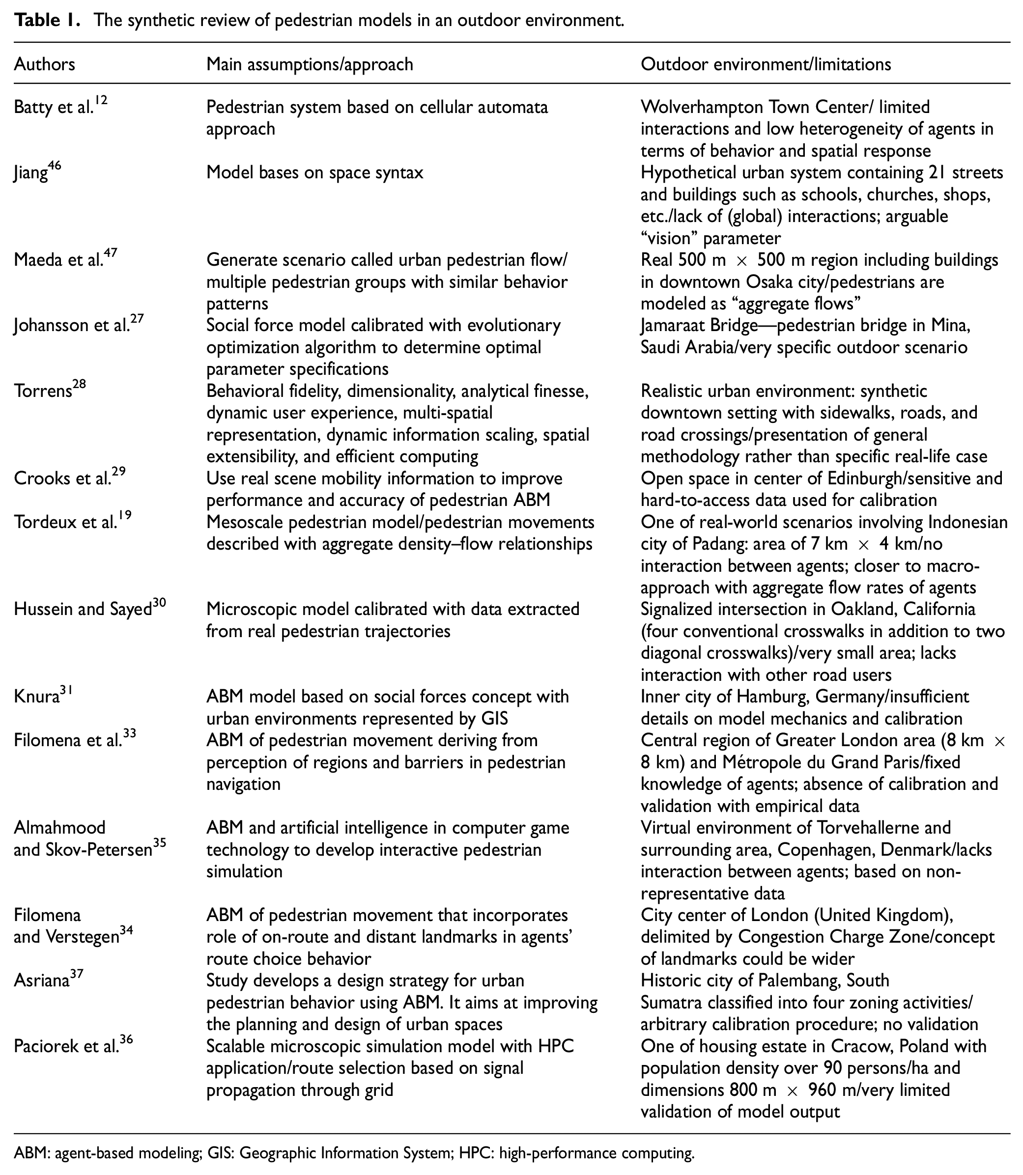
ABM: agent-based modeling; GIS: Geographic Information System; HPC: high-performance computing.

3. GP as a proxy for the volume of pedestrian traffic

GP is a service provided by Google as part of Google Maps, offering users access to a vast amount of rich place data for over 200 million POIs.⁴⁹ This service provides various features, including geocoding that converts addresses into geocoordinates, as well as access to photos and detailed information about specific places. One of the notable features of GP is the availability of place details. This feature offers a range of characteristics related to a place, such as ratings, addresses, opening hours, and popular times (including traffic data). The popular times feature displays traffic data in the form of an hourly bar chart, providing an estimate of the crowd levels at a particular place. The traffic data are derived from the localization information of mobile devices, making it relatively accurate.

For the purposes of a case study, the Old Market Square in Poznań, Poland, along with its surrounding historic streets, was selected as a simulation area. The Old Market Square is a regular square with each side measuring 140 m. It is located in the center of a network of streets that intersect at right angles. The area attracts both tourists interested in exploring historical sites and locals who visit the place for daily errands or to enjoy a café. The Old Market Square is easily identifiable on Google Maps and has its dedicated GP service, providing detailed information and insights about the location (see Figure 1). To approximate pedestrian traffic in the area with the simulation model, the popular times data from GP were used.

Figure 1.

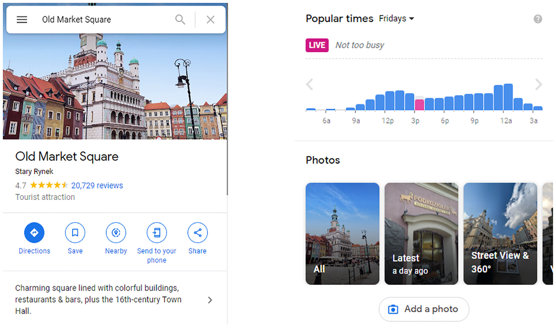
Google Places—Old Market Square in Poznań.

GP provides application programming interface (API) for basic data, the available requests include also pedestrian traffic data (popular times). To extract popularity scores, we used recent R populartimes package by Parry.⁵⁰ Populartimes provides access to the GP nearby and detail API endpoints. It also retrieves popular time data, if available and requested. The data come with a predefined scale from 0 to 100, where 0 means the lowest pedestrian traffic and 100 means the largest traffic. Figure 2 presents pedestrian traffic in the Old Market Square for 7 days of the week and 24 h starting from morning.

Figure 2.

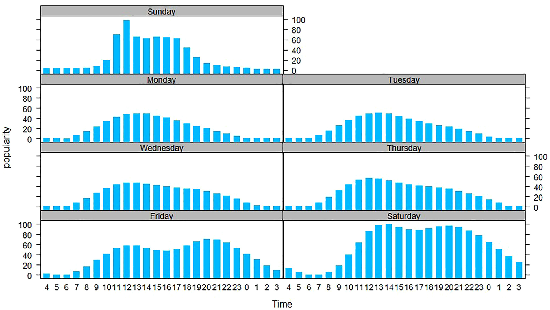
Pedestrian traffic on the Old Market Square in Poznań according to Google Places popular times.

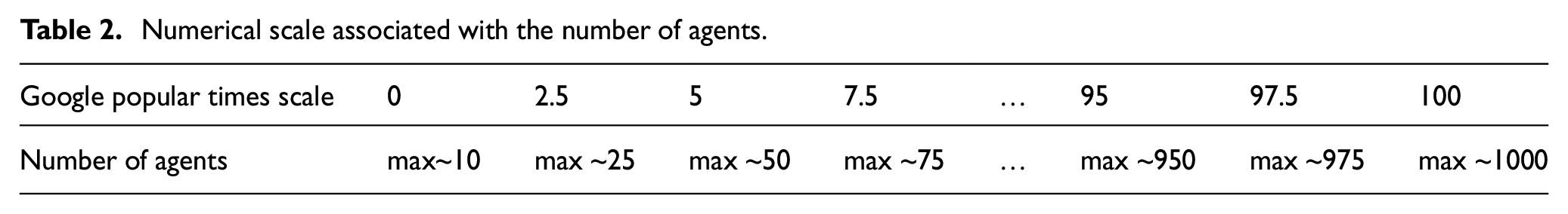
According to GP, maximal values of pedestrian traffic are observed on Sunday and Saturday between 12 p.m. and 1 p.m. These time data correspond to traffic density equal to 100. On the contrary, minimum values are observed in early mornings on Friday and Saturday, which corresponds to close to zero values. The estimates are based on average popularity of the place; however, Google does not include the information on the real number of pedestrians that is associated with specific time (https://support.google.com/business/answer/6263531?hl=en). Therefore, we had to associate the values from Google popular times scale with the specific numbers of pedestrians. We used census data on the number of inhabitants of the Old Town quarter obtained from the Web Map Service of the Poznań City Hall (The WMS server is available at: http://sip.geopoz.pl/sip/uslugi/get_uslugi_lay/. The data are official statistical data collected during national census). The Old Town quarter is inhabited by 1421 citizens in total. As our simulation sandbox covers two-third of the area, we assumed that the maximum value for pedestrian traffic is 1000 persons, which is an approximation. Not all inhabitants are on the streets at the same time, but one has to include also some number of tourists or pedestrians from other quarters or districts. However, more accurate data on this issue are unavailable.

The precise values for the number of pedestrians were adjusted according to the scale from GP (0–100). These values are assumed to be maximal values of pedestrian traffic, i.e., the number of pedestrians can be lower but it should not exceed the threshold values. However, the model has both stochasticity as well as inertia, thus, slight deviations from the threshold numbers are possible, which in fact is closer to real live conditions. For convenience, in the first interval, we assumed the maximum number of pedestrians to be 10. In this case, there is a possible situation with 0 pedestrians in the simulation; however, it should not be (much) more than 10 of them (see Table 2).

Table 2.

Numerical scale associated with the number of agents.

Google popular times scale	0	2.5	5	7.5	…	95	97.5	100
Number of agents	max~10	max ~25	max ~50	max ~75	…	max ~950	max ~975	max ~1000

4. The model of pedestrian traffic

4.1. General assumptions and sandbox details

We consider recreational and touristic walking patterns during non-working days (Sunday); commuting, shopping, running errands, etc. are skipped due to the specificity of pedestrian dynamics during this day. We chose Sunday because the day is characterized by a whole range of pedestrian traffic values (from minimal values observed in the early morning to maximal values observed about noon). We assume that Sunday is an average Sunday, with common weather conditions and no unpredictable events that may disturb regular traffic.

The general mechanics of agents’ movement rests on the gradient method described by Dietrich and Köster⁵¹ and used by Crooks et al.²⁹ We also drew on our previous works.^52,53 This approach assumes that each agent is seeking one destination point. The closer the agent is to the point, the stronger he or she is attracted by it. In this case, these POIs are shops, cafes, museums, or other amenities available in the Old Town area.

The agents are born in the entry points. The higher the pedestrian traffic declared by GP data, the higher the probability of creating new pedestrians. Similarly, if the agents want to exit the simulation, they randomly select one of the exit points and navigate to it. If they reach the point, they permanently leave the sandbox. The concept is similar to the gateways described by Knura³¹ or Filomena et al.³³ However, we did not associate probability values with entry/exit points as in the study of Crooks et al.²⁹ In the model, the gateways are situated in the locations linked to transport (tram, bus stops) as well as parking facilities. In general, pedestrian flows are usually observed from and to these points. Bidirectional pedestrian flows are modeled as the agents can simultaneously move in any direction.

The simulation sandbox is the Old Market Square in Poznań with the surrounding historic streets. The side of the area has approximately 450 m with the diagonal equal to 636 m. In Figure 3, the left panel is a Google Maps satellite photo, the right panel shows extracted polygons with entry/exit points and dimensions of the simulation area.

Figure 3.

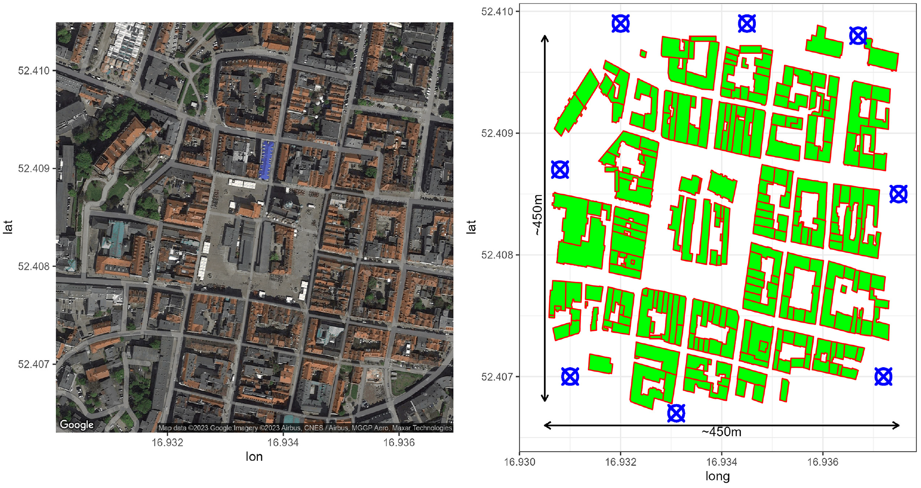
Old Market with the surrounding streets—Google Maps view and the extracted polygons used in simulation. On the right panel, circles with crosses are the entry/exit points.

4.2. Controlling for time and traffic

Each side of the simulation box has 201 equal patches. Thus, the total area is 40,401 patches. The length of a single patch corresponds to 2.25 m (450 m is 200 patches). On the basis of a single patch length, the preferred speed of agents was adjusted to one patch per tick. It means that during each simulation step (tick), the agent can traverse a maximum of one patch (2.25 m).

The preferred human pace during walking activity is ~1.4 m/s (~5 km/h; The preferred walking speed is the speed at which humans or animals choose to walk. According to research, many people tend to walk at about 1.4 m/s; Mohler et al.⁵⁴). Therefore, to traverse 2.25 m (one patch) at the preferred speed human needs 1.6 s. Combining it with one simulation step means that it covers ~1.6 s of the real time as the agent traverse 2.25 m/tick. Therefore, 1000 ticks are comparable with 1600 s (26 min). A total of 2250 ticks are approximately 1 h.

Agents may roam the space with lower speed according to the principles of navigation described in the next subsection. We used excellent NetLogo time extension by Collin Shepard (The extension and Quick Start Guide are available at: https://github.com/colinsheppard/time) to set and manage the exact daytime in the simulation. According to the previous derivation, the value of 1.6 s was anchored to one simulation tick. The simulation starts on Sunday at 4 a.m., ends on Monday at 4 a.m., and covers 24 h, which makes up 54,000 ticks in the simulation sandbox.

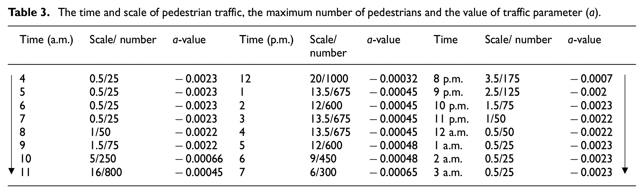
The number of pedestrians in the simulation evolves according to agent creation and agent destruction conditions. The births of new pedestrians are possible only at the entry points and take place with an endogenous creation formula. If the number of agents is lower than the threshold value provided by GP data, the given number of agents (This number is drawn at random from 1 to 10 interval) is created with the probability equal to (However, if the number of agents is higher than the threshold provided by GP, parameter a switches to a/2, and if it is lower, a turns to a×2) as follows:

λ_{t} = 1 - e^{- a_{t} \times * N_{t}}

(1)

Therefore, the λ strongly depends on the total number of agents in the simulation (N) and parameter $a$ . As the number of agents rises, the probability also rises. Parameter $a$ dynamically changes during the daytime and depends on an hour. The more agents in the simulation, the smaller the parameter $a$ is to keep λ in a reasonable threshold. Consequently, the birth or the creation rate of agents $γ$ is as follows:

γ_{t} = \frac{n_{t}}{N_{t}},

(2)

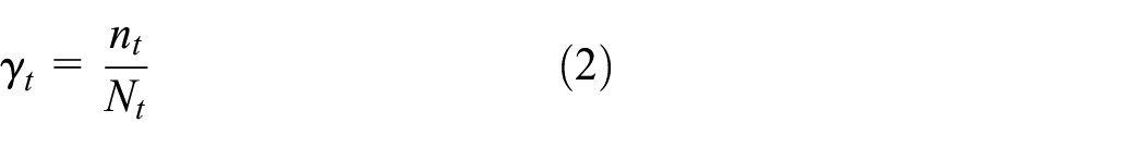
where n is the inflow of new agents to the simulation. Consequently, the agents leave the simulation when they locate the target and then complete the route to the chosen exit point. Each agent decides which exit to choose and how to navigate to it, therefore the pedestrians disappear with some endogenous rate $δ$ as follows:

δ_{t} = \frac{d_{t}}{N_{t}},

(3)

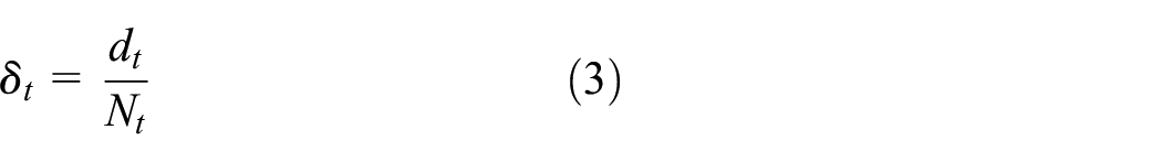
where d is the number of agents leaving simulation. The system is in the equilibrium if the condition $γ_{t} = δ_{t}$ is fulfilled. However, such situations may be momentary as the simulation constantly evolves according to the actual state and conditions 1–3. If $γ_{t} > δ_{t}$ , the number of agents rises. If $γ_{t} < δ_{t}$ , the number of pedestrians decreases. From this perspective, the proper choice of value of parameter $a$ is the key element of providing reasonable fluctuations in pedestrian movements as well as the accurate number of agents roaming the Old Market Square. The parameter values were adjusted according to the grid-search procedure. We carried out multiple repetitions of the simulation to find proper a values that kept the number of agents in a range provided by GP data. In Table 3, we included the values of parameter $a$ for a given traffic size and hour.

Table 3.

The time and scale of pedestrian traffic, the maximum number of pedestrians and the value of traffic parameter (a).

Time (a.m.)	Scale/ number	$a$ -value	Time (p.m.)	Scale/number	$a$ -value	Time	Scale/ number	$a$ -value
4	0.5/25	−0.0023	12	20/1000	−0.00032	8 p.m.	3.5/175	−0.0007
5	0.5/25	−0.0023	1	13.5/675	−0.00045	9 p.m.	2.5/125	−0.002
6	0.5/25	−0.0023	2	12/600	−0.00045	10 p.m.	1.5/75	−0.0023
7	0.5/25	−0.0023	3	13.5/675	−0.00045	11 p.m.	1/50	−0.0022
8	1/50	−0.0022	4	13.5/675	−0.00045	12 a.m.	0.5/50	−0.0022
9	1.5/75	−0.0022	5	12/600	−0.00048	1 a.m.	0.5/25	−0.0023
10	5/250	−0.00066	6	9/450	−0.00048	2 a.m.	0.5/25	−0.0023
11	16/800	−0.00045	7	6/300	−0.00065	3 a.m.	0.5/25	−0.0023

4.3. Principles of navigating

The navigation is made as easy as possible. Artificial pedestrians regulate speed and distance from other agents. They avoid collisions by choosing the patches that are not settled by other agents. Each pedestrian starts the simulation with speed = 1 patch/tick (1.4 m/s or 5 km/h), then speed evolves according to the behavioral rules described below. Agents, however, tend to travel at the preferred speed of 5 km/h, which, by assumption, cannot be exceeded. There is also a lower speed threshold which we set at 0.2 patch/tick. It means that speed cannot fall below 0.3 m/s (1 km/h), which can be considered as a very slow walk.

Figure 4 presents three main principles of interactions with other pedestrians. Principle A of collision avoidance says that each agent has a vision distance = two patches in his or her moving direction. If the agent identifies another pedestrian coming from the opposite direction, he or she turns randomly by 15°. However, under heavy traffic, if principle A cannot be fulfilled the agent just choose the nearest patch at an angle of 180°, which is free (principle B). Principle C says that agents dynamically adjust the pace to other pedestrians that move in the same direction. If other walkers are too close, the agent adjusts speed to the speed of the nearest pedestrian and slows down to maintain the distance.

Figure 4.

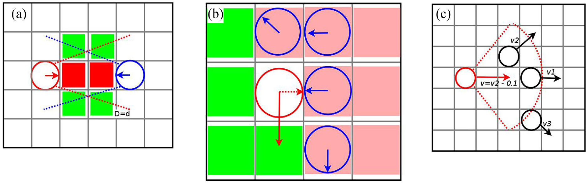
(a) Collision avoidance, (b) heavy traffic management, and (c) speed adjustment.

Each agent choses the route on the basis of the calculation of patch values $(μ)$ . These values are calculated according to the formula as follows:

\begin{matrix} μ = s - d * θ \\ θ ~ N (M, SD) \end{matrix}

(4)

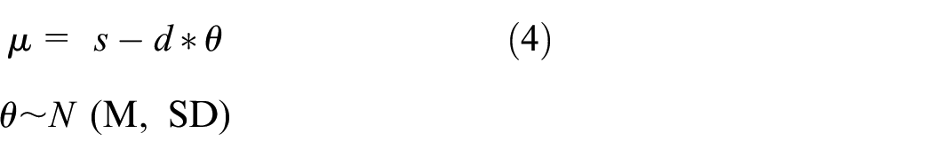
where s is the value of a destination patch; d is the distance in patches from the destination; $θ$ is a random parameter whose values are drawn for each agent from normal distribution with a given mean and standard deviation every 40 ticks (If the drawn number is lower than 0, then the value is set at 0. In this special case, the value of all patches is equal for the agent, and he or she randomly roams the space until the next drawing changes the value). However, if one of the walkable patches shares at least one border with a building or other obstacles, the value of such a patch is diminished by exogenous discount rate $r$ according to the formula as follows:

μ = (s * r) - d * θ

(5)

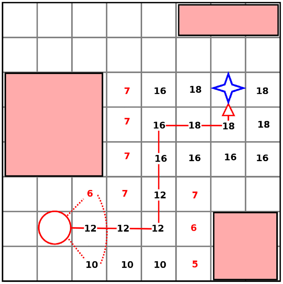
To decrease the computational demand of the model, the agents calculate values of patches only in a given range ahead. Mainly, during each simulation step, the pedestrian calculates values for six patches, which are in front of him or her. Assuming $s = 20, θ = 2$ and $r = 0.5$ , the calculation of values of patches for a given target would look like as shown in Figure 5.

Figure 5.

Route choice on the basis of values of patches. Red rectangles are obstacles that diminish values of patches; the blue star is the destination patch; numbers are values of patches computed based on formulae (4) and (5).

4.4. Calibration

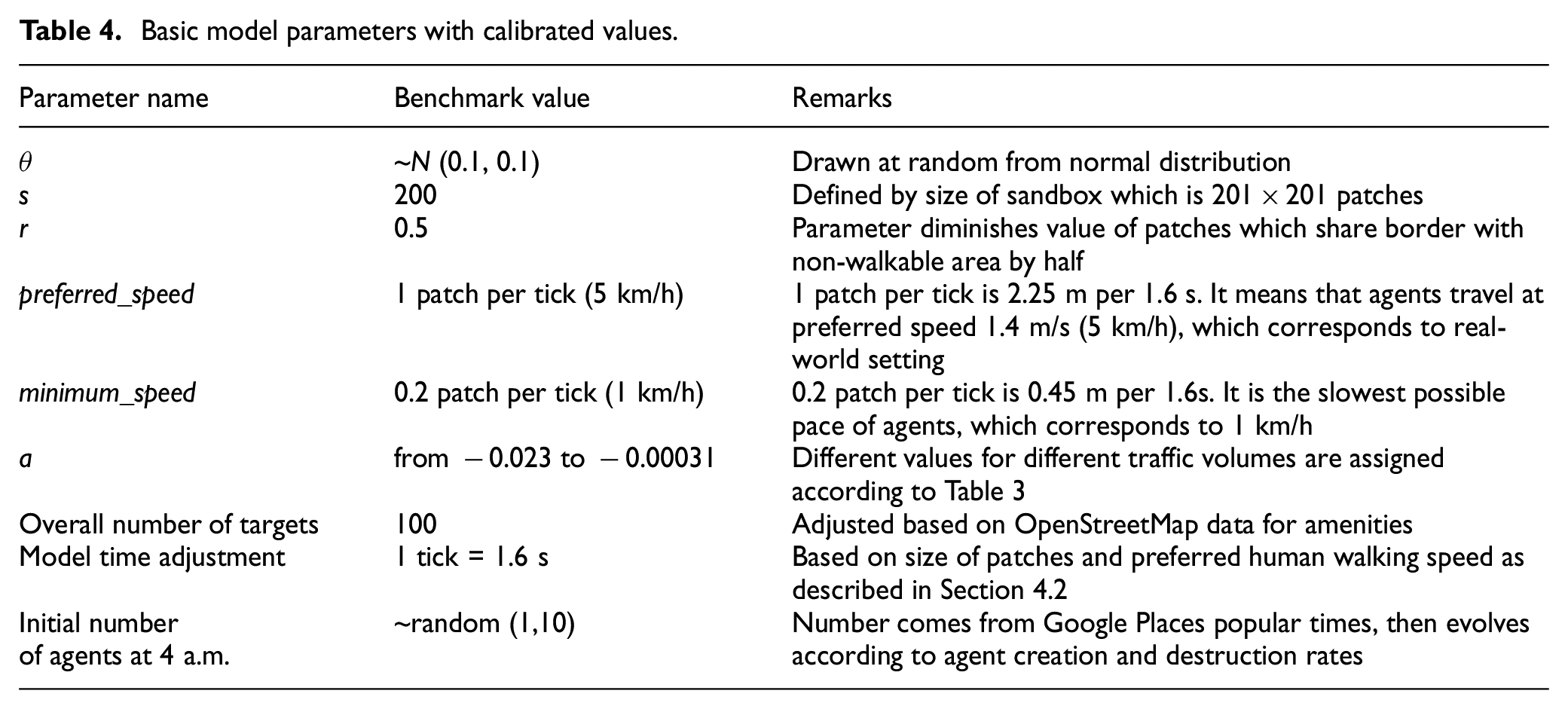
Apart from the job creation rate that relies on λ and the value of pedestrian traffic parameter (a), the model consists of some other inputs that affect walking decisions. The number of parameters is rather small, as we present a mesoscopic perspective and avoid some low-level pedestrians’ interactions.

The next important parameter is $θ$ that governs the decisions about assigning values to patches. $θ$ diminishes the attractiveness of patch by some fixed value depending on the distance. Therefore, it should be set somewhere between 0 and 1 interval. If $θ$ is 0, all patches have equal values and the agents walk at random. If gravity is equal to 1, the attractiveness of patch is diminished by the full distance to the destination. Thus, normal distribution with mean equal to 0.1 and standard deviation equal to 0.1 were chosen to sampling gravity for each agent. The individual differences in $θ$ reflect different walking strategies as the parameter directly impacts walking behavior (lower values of gravity are associated with recreational, unhurried walk; higher values are associated with rush to the target). According to Open Street Maps, there are 60 pubs and restaurants as well as 43 shops of different kinds in the Old Market Square. Consequently, the number of targets for agents was set at 100. The list of all parameters included in the model with benchmark values is presented in Table 4.

Table 4.

Basic model parameters with calibrated values.

Parameter name	Benchmark value	Remarks
$θ$	~N (0.1, 0.1)	Drawn at random from normal distribution
s	200	Defined by size of sandbox which is 201×201 patches
r	0.5	Parameter diminishes value of patches which share border with non-walkable area by half
preferred_speed	1 patch per tick (5 km/h)	1 patch per tick is 2.25 m per 1.6 s. It means that agents travel at preferred speed 1.4 m/s (5 km/h), which corresponds to real-world setting
minimum_speed	0.2 patch per tick (1 km/h)	0.2 patch per tick is 0.45 m per 1.6s. It is the slowest possible pace of agents, which corresponds to 1 km/h
a	from −0.023 to −0.00031	Different values for different traffic volumes are assigned according to Table 3
Overall number of targets	100	Adjusted based on OpenStreetMap data for amenities
Model time adjustment	1 tick = 1.6 s	Based on size of patches and preferred human walking speed as described in Section 4.2
Initial number of agents at 4 a.m.	~random (1,10)	Number comes from Google Places popular times, then evolves according to agent creation and destruction rates

4.5. Benchmark simulations

The simulations were performed in NetLogo 6.0.4 and R 4.1.0 together with RNetLogo 1.0–4 extension.⁵⁵ As was mentioned earlier, we also used NetLogo time extension⁵⁶ to manage time in simulation and NetLogo GIS extension^57,58 to set up and manage a GIS environment (Shapefiles were prepared with QGIS3 and OSM plugins). Figure 6 presents a cross-correlation plot for the major model outputs that we analyze and assess in the further steps of the research procedure. The average speed in the simulation was 0.83 patch/tick (4.17 km/h). The higher the number of agents, the lower the speed (significant dependency is observed through the correlation score and scatterplot). This negative relationship has been confirmed in several empirical studies (Pinna and Murrau⁵⁹). Speed also falls together with increased agents’ inflow and time that agents spent in the simulation. The average time spent in the simulation was 11 min; the minimum time was less than a minute and the maximum time was about 62 min.

Figure 6.

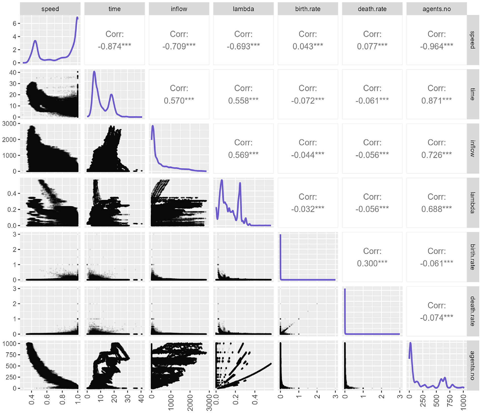
Pairplot for model generated output. Upper panel shows a cross-correlation score between variables; diagonal panel shows density plots; lower panel shows scatterplots; plots were produced based on 10 simulations.

The mean number of pedestrians is reported to be 249, with a minimum value of 0 and a maximum value of 1008. This indicates a significant variation in pedestrian presence during different time periods. It is worth noting that the model demonstrates a positive relationship between the number of pedestrians and travel time or the flow of agents, which aligns with findings from empirical research, such as the study conducted by Tipakornkiat et al.⁶⁰ The boxplots in Figure 7 provide a visual representation of the distribution of pedestrian agents across different hours. They offer insights into the variability and trends in pedestrian traffic throughout the day.

Figure 7.

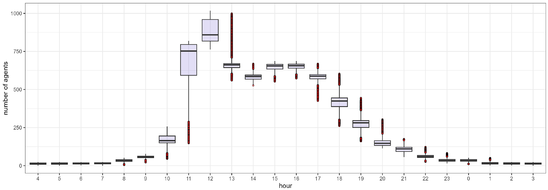
Boxplots for the number of agents by hour. Reported values make up the average of 10 simulations.

The model captures the complex mechanisms behind the immediate changes in pedestrian quantities, whereas GP data primarily reflects the intensity of pedestrian traffic. The maximum number of agents is observed between 12 p.m. and 1 p.m., with the peak closer to 1 p.m. due to the time it takes for the area to fill with agents. As the number of pedestrians increases, the inertia of the crowd rises, leading to longer adjustment times for the model. This is influenced by the limited capacity of the area and the location of entry/exit points, which pose challenges for route finding as bidirectional flows intensify.

Figure 8 displays pedestrian trajectories and densities during selected hours, showing significant variations in the number of pedestrians. Between 8 and 9 a.m., the pedestrian count remains below approximately 50, increasing to around 75 between 9 and 10 a.m. A significant rise to approximately 250 pedestrians occurs between 10 and 11 a.m., with a peak of around 1000 pedestrians between 12 and 1 p.m. After 2 p.m., the number gradually decreases to a maximum of around 600, stabilizing at approximately 450 pedestrians around 5 p.m. These findings demonstrate the model’s ability to capture the complex dynamics and fluctuations in pedestrian numbers throughout the day in the city center, providing deeper insights into pedestrian behavior than GP data alone.

Figure 8.

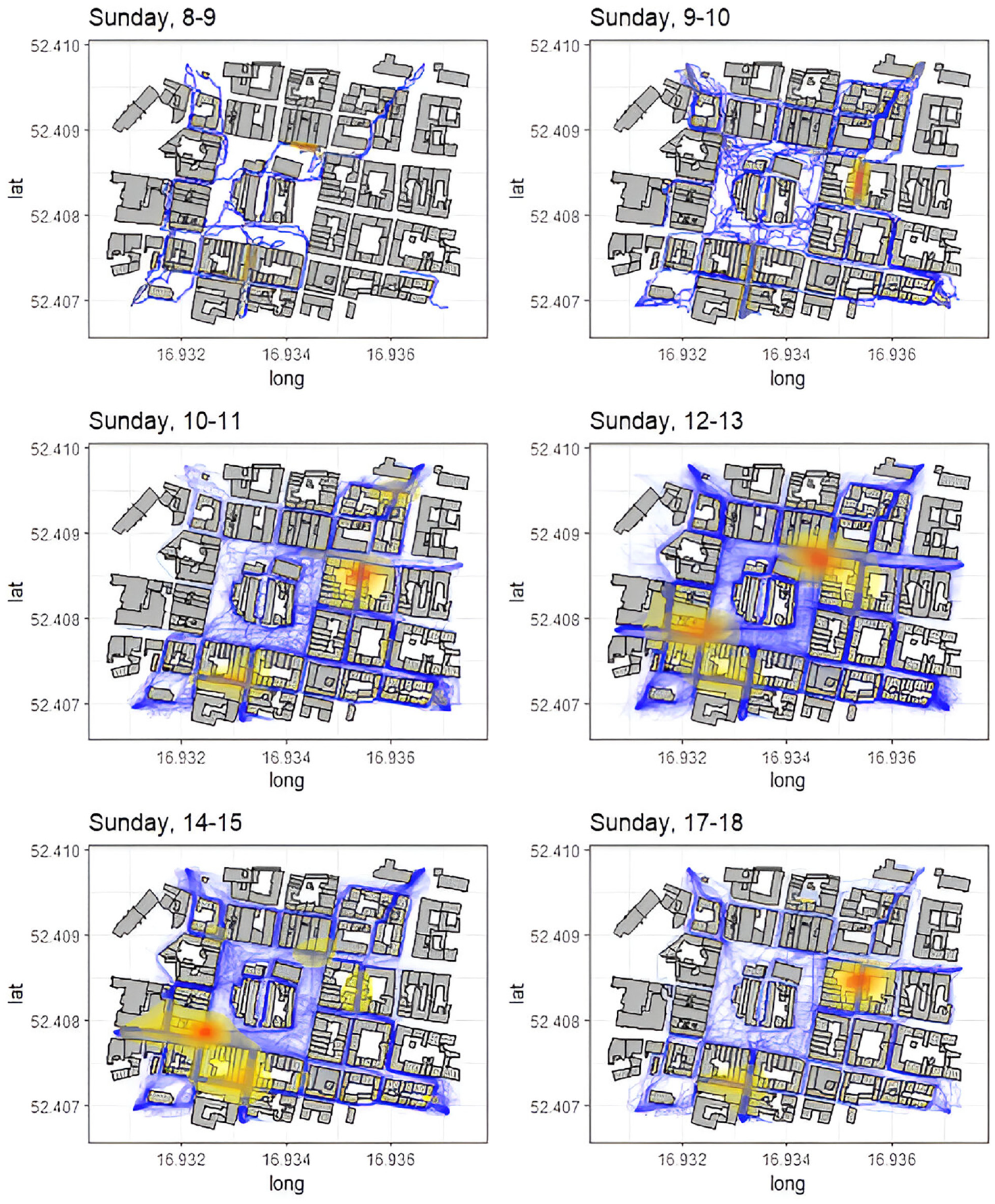
Agents’ trajectories and densities for selected hours during the daytime.

During Sunday morning (8–11 a.m.), popular pedestrian routes are observed from the southern to the northern part of the area. The historic streets in the southern and eastern areas experience increased pedestrian density. The highest density of pedestrian traffic occurs between 12 and 1 p.m., particularly in the streets leading to transportation and parking facilities located in the bottom left and upper right quarters of the simulation area. During peak hours, congestion zones shift from the historic streets to areas where pedestrians are entering or leaving the Old Market Square and navigating through narrow surrounding streets. This phenomenon represents a bottleneck scenario in the outdoor environment with natural obstacles, confirming observations from empirical studies such as Campanella et al.⁶¹ or Luo et al.⁶² Figure 9 illustrates the speed and density in specific quarters of the simulation area, providing further insights into the dynamics of pedestrian flow.

Figure 9.

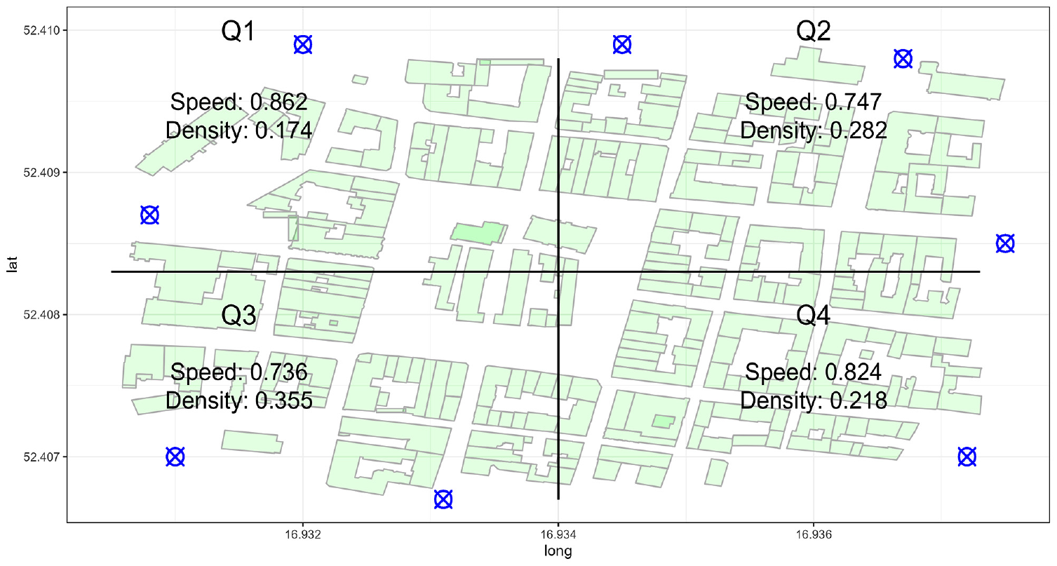
Agents’ average speed and density in the quarters of the Old Market Square during the day. Blue circles with crosses are the entry/exit points.

The quarter with the highest speed (Q1) also exhibits the lowest density of agents. This can be attributed to the relatively small area covered by historic streets in Q1, along with the greater distance between entry/exit points. On the contrary, the quarter with the highest density (Q3) is associated with slower speeds, as indicated by the heatmaps in Figure 8. Q3 experiences increased density because of two entry/exit points located in close proximity, resulting in agents choosing a common route and creating a bottleneck. Q2, characterized by the second slowest speeds, may be influenced by both the larger area covered by historic streets and the presence of three entry/exit points in this quarter. Q4 also exhibits low density and high speed, which can be attributed to having only one entry/exit point located in this quarter. Figure 10 provides additional insights through line plots of birth and death rates of pedestrians (lambda) per minute, as well as a bar plot showing the inflow of new agents.

Figure 10.

Probability of the creation, birth and death rates of agents together with an inflow of agents per minute. Birth rate is the number of new turtles in simulation/minute/the total number of turtles; death rate is the number of turtles leaving the simulation/minute/total number of turtles; the red line is a LOESS regression curve for highly volatile time-series; reported values make up the average of 10 simulations.

The birth and death rates drop as the probability of agents creation (λ) rises; both rates also highly depend on the number of agents in the simulation as well as the number of agents entering and leaving the sandbox, while λ evolves together with hourly adjusted parameter a. These rates are lower for the hours with the higher number of pedestrians and higher if the number of simulated pedestrians decreases (As both rates are the result of division by the number of agents in the simulation area, they drop together with the increased traffic). It can be also observed that these indicators share a common trend and similar values. This means that if the number of agents entering the simulation is large, also the number of agents leaving the simulation is large (and vice versa). The probability of agents’ creation rises during the most popular hours of the day to fulfill the traffic intensity conditions provided by GP data. The inflow of new agents per minute is highly cyclical. Despite the generation of the day trend, the inflow fluctuates significantly over minutes. Usually the minutes with a lower inflow are followed by the minutes with a higher inflow. This phenomenon could be interpreted as pedestrian waves resulted from the public transportation arrivals as described by Gorrini et al.⁹ Then, in Figure 11, we present inflow of agents in the Old Market square per hour together with the cumulative sum of pedestrians during the daytime.

Figure 11.

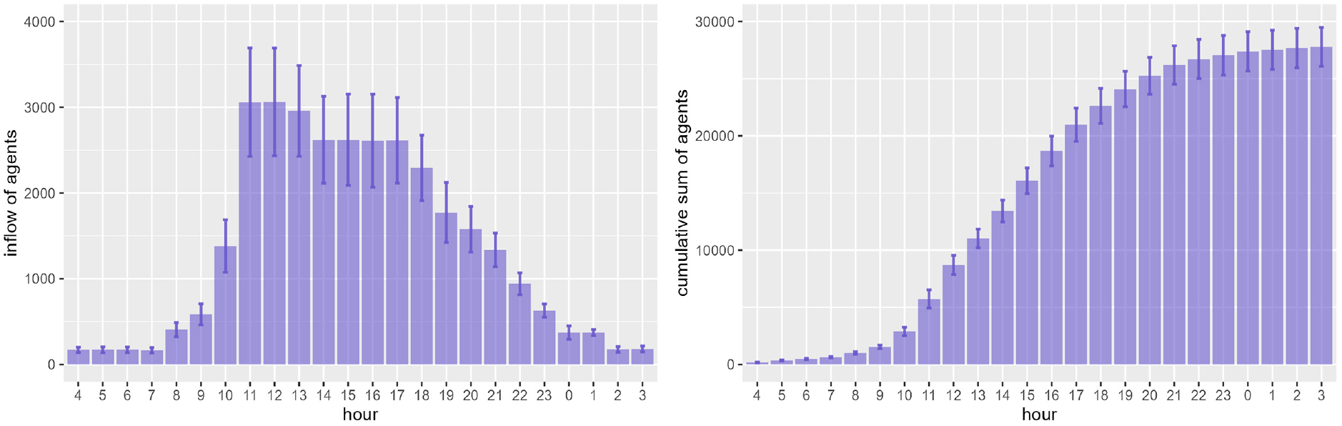
The inflow of agents and the cumulative sum of pedestrians per hour. Bars show standard deviation; reported values make up the average of 10 simulations.

The total average capacity of the area on Sunday was about 28,000 agents (there are, however, simulation runs with lower and higher capacities as shown by error bars). The highest inflow of new pedestrians was observed between 11 a.m. and 1 p.m. In that time 3000 pedestrians per hour arrived at the city center (on average). The standard deviation for the pedestrian inflow is large and shows that the size of the pedestrian flow varies significantly during given time periods (e.g., during peak hours, the flow of 2300–3800 pedestrians was observed). The hour of the highest inflow (11 a.m.–12 p.m.) preceded the hour of the highest pedestrians’ density (12 p.m.–1 a.m.) as it takes some time to fill the area with a given number of agents. Therefore, the highest load of public transport and parking facilities on Sunday could be expected between 10 a.m. and 1 p.m.; however, an intensified pedestrian flow may be observed up to 7 p.m.–8 p.m. Finally, Figure 12 plots the average speed of agents and time they spent in the simulation.

Figure 12.

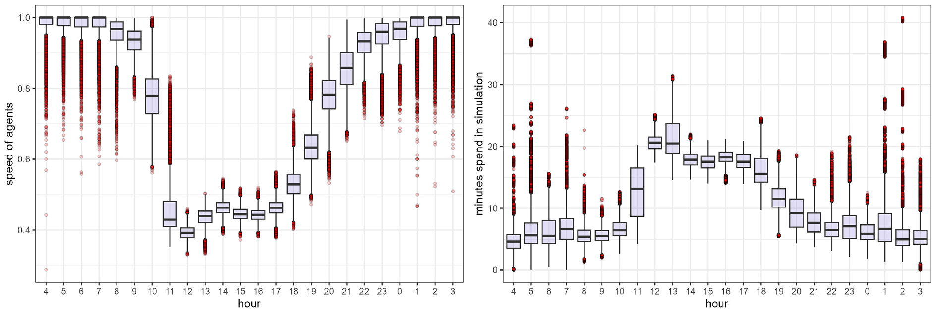
Boxplots for speed (patches/tick) and time the agents spent in the simulation by hour. Reported values make up the average of 10 simulations.

The agents travel around the preferred speed up to 10 a.m. Then, because of increased density, they reduce their speed by 20%–30%. The lowest average speed is observed between 11 a.m. and 4 p.m. It is connected with higher pedestrians’ density that intensifies before midday and lasts till afternoon. In addition, the average speed drops fast between 250 and 800 agents; however, the further increase in the number of agents does not impact the speed so significantly. The mean speed during the daytime was 3.96 km/h (1.1 m/s) with the standard deviation equal to 1.12 km/h (0.31 m/s). The larger standard deviation means larger diversity of individual speeds. The standard deviation drops during peak hours and is higher for neighboring time periods that have larger differences in the number of pedestrians, e.g., transition from 250 to 800 agents (10–11 a.m.) is associated with the highest standard deviation. It may be the result of intensified pedestrian flows that increase speed heterogeneity as noted by Yang et al.⁶³ During the peak hours, agents spend the longest time in the simulation (up to 25 min) but the mean value is about 11 min (with the standard deviation equal to 5.8 min). The empirically measured time to cross the simulation area from the northern to the southern exit point was about 5 min. According to GP, people spent up to 30 min at the Old Market Square.

4.6. Model validation

In this study, the validation method used is limited by the availability of real-life data, but still meets the requirements established during the model creation process. The validation process involves comparing the model output with the existing empirical contributions on pedestrian traffic as well as data obtained from GP. To evaluate the model’s performance, we selected four different POIs located in the Old Market Square and the surrounding streets. These POIs include the Old Market Square (in general), the Poznań Museum (Detailed coordinates for Town hall Poznan museum: 52.40926746157, 16.9341414883), the Chocolate Café (Detailed coordinates for Chocolate Café (orig. Café Czekolada): 52.40898679634, 16.9339130928), and one of the groceries’ stores (Detailed coordinates for Żabka grocery store: 52.40741166852, 16.9342671056). However, it should be noted that these places have different opening hours, which means we could only evaluate the pedestrian traffic during specific periods when the data were available.

Figure 13 presents the mean value of pedestrian traffic generated by the model compared to the data obtained from the popular times rank at the specific POIs. This comparison makes it possible to assess how well the model aligns with the observed pedestrian traffic patterns at these locations.

Figure 13.

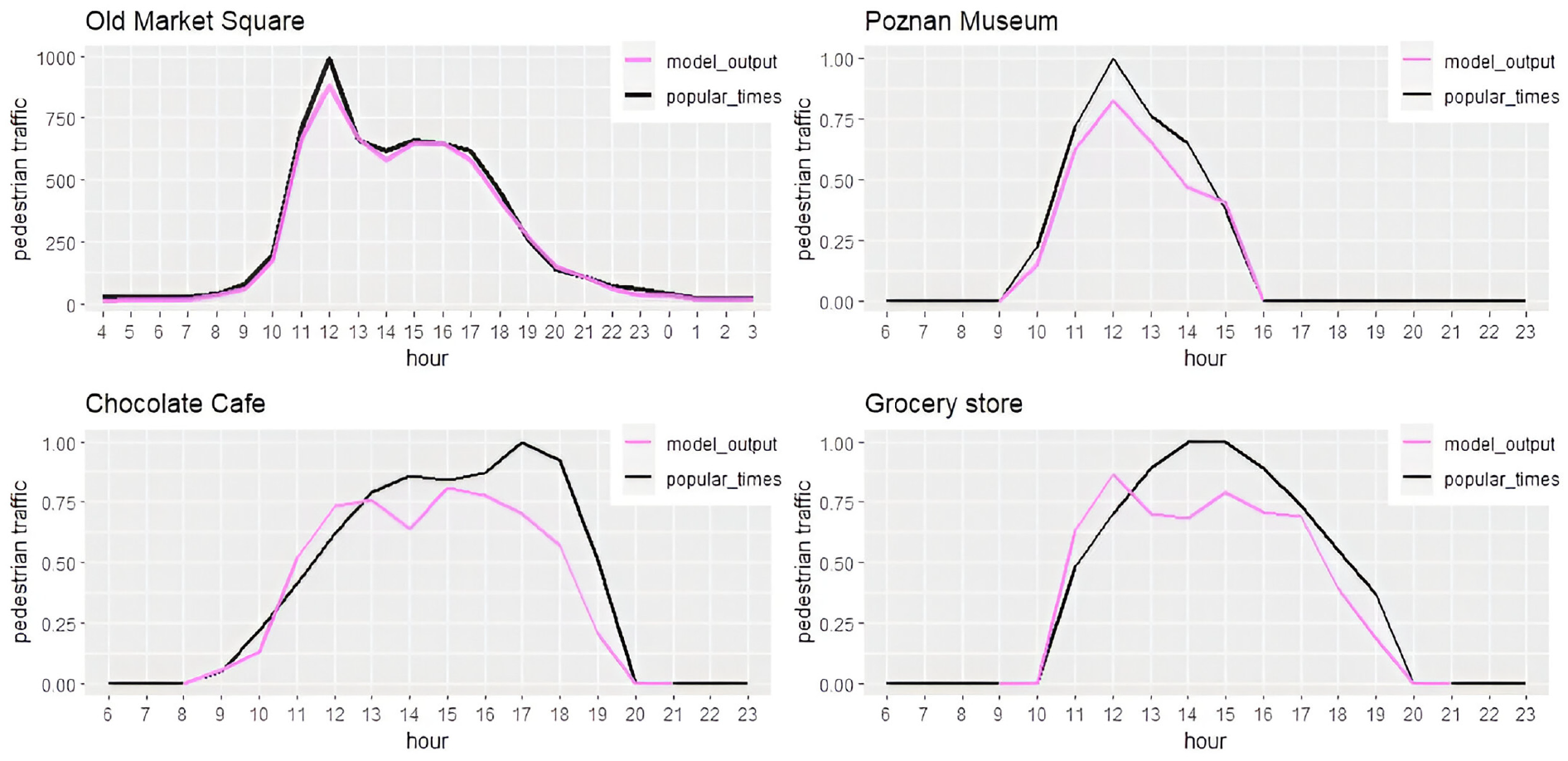
Evaluation of the model-generated traffic against popular times data at the selected POIs.

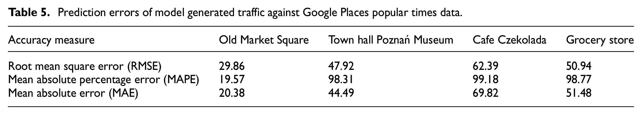
The model replicates the general dynamics of pedestrian traffic at all selected places; however, there are some significant differences regarding the precision of the replication. The best accuracy is kept at the Old Market Square (as the average traffic around the square), good results was also obtained for Poznan museum, which is located at the Old Market Square. Less accurate estimations were observed at Cafe Czekolada and the grocery store that are located outside the central place at the historic streets surrounding the market. Table 5 presents model prediction errors at the selected POIs.

Table 5.

Prediction errors of model generated traffic against Google Places popular times data.

Accuracy measure	Old Market Square	Town hall Poznań Museum	Cafe Czekolada	Grocery store
Root mean square error (RMSE)	29.86	47.92	62.39	50.94
Mean absolute percentage error (MAPE)	19.57	98.31	99.18	98.77
Mean absolute error (MAE)	20.38	44.49	69.82	51.48

In order to validate the model, we also conducted a comparison between the model-generated outputs and previous empirical works. One key aspect we examined was the relationship between pedestrian density and speed, which has been investigated by Virkler and Elayadath⁶⁴ using seven different models. They found a significant negative correlation between these two variables, and our model confirms this finding, with a correlation coefficient of –0.96 (see Figure 6). This dependency is consistent with the results of Nikolić et al.⁶⁵ and aligns with fundamental diagrams of pedestrian flows as observed in studies by Campanella et al.,⁶⁶ and Vanumu et al.⁶⁷

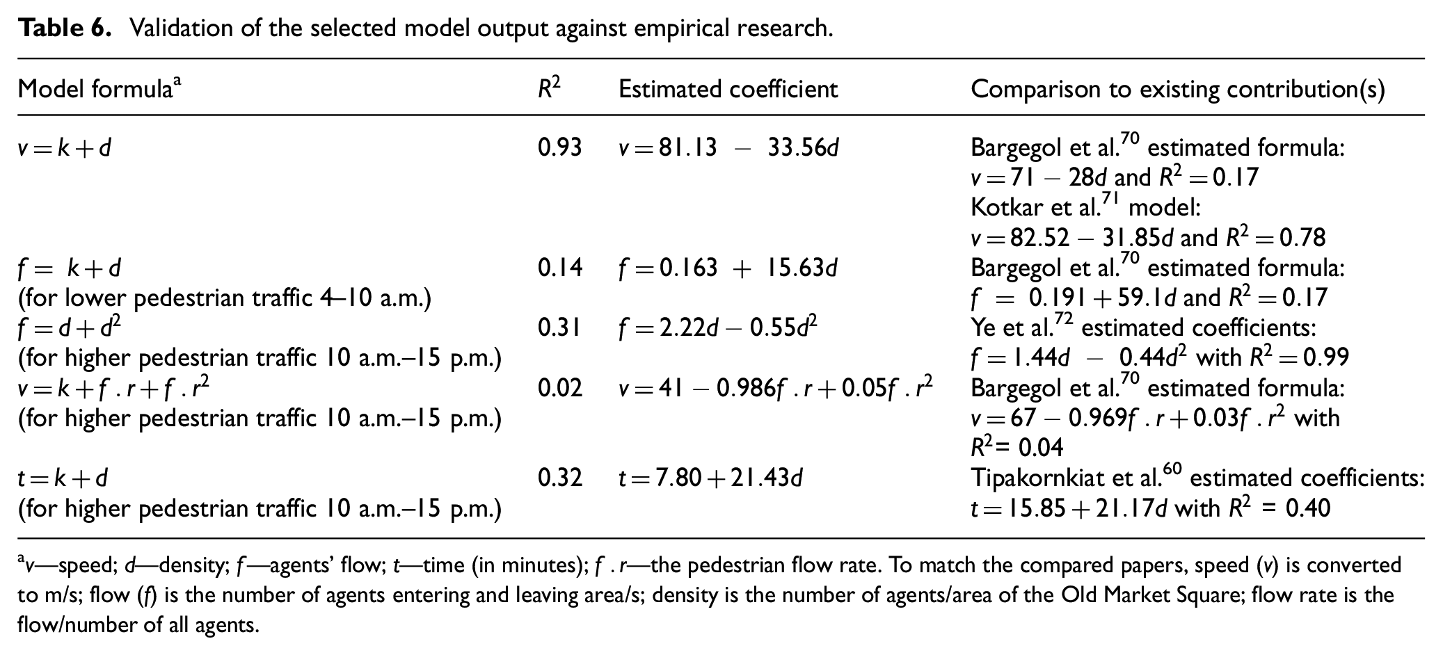
During rush hours, we identified two significant bottlenecks occurring in the areas connecting the Old Market Square and the narrow historic streets. These bottlenecks result from bidirectional pedestrian flows and increased pedestrian density, which aligns with the findings of Campanella et al.⁶¹ and Luo et al.⁶² Furthermore, our model revealed that during periods of increased pedestrian inflow (10 a.m.–12 p.m.), the speed became more diversified, indicated by a larger standard deviation. This phenomenon can be attributed to intensified bidirectional pedestrian flows, as noted by Yang et al.⁶³ We observed a speed standard deviation of 0.31 m/s with a mean speed of 1.1 m/s, which corresponds to previous findings under similar external conditions. For instance, Lam et al.⁶⁸ reported a mean speed of 1.19 m/s with a standard deviation of 0.26 m/s in an urban outdoor environment. Similarly, Older⁶⁹ observed a mean speed and standard deviation of 1.3 and 0.3 m/s, respectively, in European shopping streets, which closely aligns with our model output. In validating the model, the study by Bargegol et al.⁷⁰ proved particularly useful. Although their investigation focused on urban intersections, we identified similarities between our model output and their findings regarding speed–flow rate dependencies. In addition, we referred to the work of Kotkar et al.,⁷¹ who conducted empirical research on pedestrian flows in sidewalk locations in medium-sized cities. Other valuable references include the study by Ye et al.,⁷² who estimated density coefficients based on observations of pedestrians in one-way passageways, and Tipakornkiat et al.,⁶⁰ who investigated time–density relationships on sidewalks in Bangkok. Table 6 presents a comparison between the results of these studies and our model output.

Table 6.

Validation of the selected model output against empirical research.

Model formula^a	$R^{2}$	Estimated coefficient	Comparison to existing contribution(s)
$v = k + d$	0.93	$v = 81.13 - 33.56 d$	Bargegol et al.⁷⁰ estimated formula: $v = 71 - 28 d$ and $R^{2} = 0.17$ Kotkar et al.⁷¹ model: $v = 82.52 - 31.85 d$ and $R^{2} = 0.78$
$f = k + d$ (for lower pedestrian traffic 4–10 a.m.)	0.14	$f = 0.163 + 15.63 d$	Bargegol et al.⁷⁰ estimated formula: $f = 0.191 + 59.1 d$ and $R^{2} = 0.17$
$f = d + d^{2}$ (for higher pedestrian traffic 10 a.m.–15 p.m.)	0.31	$f = 2.22 d - 0.55 d^{2}$	Ye et al.⁷² estimated coefficients: $f = 1.44 d - 0.44 d^{2}$ with $R^{2} = 0.99$
$v = k + f . r + f . r^{2}$ (for higher pedestrian traffic 10 a.m.–15 p.m.)	0.02	$v = 41 - 0.986 f . r + 0.05 f . r^{2}$	Bargegol et al.⁷⁰ estimated formula: $v = 67 - 0.969 f . r + 0.03 f . r^{2}$ with $R^{2}$ = 0.04
$t = k + d$ (for higher pedestrian traffic 10 a.m.–15 p.m.)	0.32	$t = 7.80 + 21.43 d$	Tipakornkiat et al.⁶⁰ estimated coefficients: $t = 15.85 + 21.17 d$ with $R^{2}$ = 0.40

$v$ —speed; $d$ —density; $f$ —agents’ flow; t—time (in minutes); $f . r$ —the pedestrian flow rate. To match the compared papers, speed (v) is converted to m/s; flow (f) is the number of agents entering and leaving area/s; density is the number of agents/area of the Old Market Square; flow rate is the flow/number of all agents.

5. Conclusion and discussion

In this paper, we developed an agent-based model to simulate pedestrian fluctuations in the city center. We calibrated parameters related to pedestrian traffic and density using data from GP popular times and Geographic Information Systems (Web Map Service). The simulation area was accurately represented using GIS data, and we paid close attention to time and speed as key elements of the simulation approach.

We aimed to bridge the gap between utilizing ABM and evaluation of pedestrian movement within built environments. Especially, we focused on properties of daily fluctuations in pedestrian traffic, which have not yet been thoroughly examined within the framework of ABM.

The model’s ability to generate intricate pedestrian flow patterns offers valuable insights into pedestrian dynamics. It provides practical information for effective pedestrian traffic management in the city. Key findings include estimating the daily pedestrian capacity of the area, determining the size and speed of pedestrian inflow and outflow, and identifying “waves” of irregular pedestrian movement characterized by periods of high inflow followed by reduced outflow. These irregularities may be linked to factors such as public transport schedules, and result from the model’s creation and destruction conditions. By considering these factors, the model aids in developing strategies for optimizing pedestrian traffic management and enhancing overall urban mobility.

The model effectively identifies lower and higher speed zones. The lower speed zones occur in transition areas between the Old Market Square and the historic streets, where pedestrian density increases. These areas experience bottleneck scenarios due to bidirectional flows, as pedestrians entering the Old Market Square have to navigate through the departing crowd. Furthermore, the presence of tram/bus stops and parking areas, represented as entry/exit points, can contribute to high-density zones and mobility challenges, particularly when these locations are in close proximity to each other. On the contrary, quarters with less frequent and more distant entry/exit points exhibit lower pedestrian density and higher average speeds. The model’s ability to identify these variations in density and speed supports understanding and managing pedestrian mobility issues in different areas of the city (different spatial context).

We validated the model using existing empirical studies and GP popular times data for four selected POI in the Old Market Square and the surrounding historic streets. We also compared the model-generated fundamental diagrams of pedestrian flow with empirical studies conducted in outdoor environments, finding close alignment in several cases.

In conclusion, the model replicates certain patterns of pedestrian dynamics and offers new possibilities for studying pedestrian fluctuations. This approach has practical implications for managing public transport and pedestrian traffic. The model is quite simple and computationally efficient, as we were able to generate results in a reasonable time frame using average class PC. However, it has also limitations. First, it relies on historical data, which means stochastic changes in pedestrian flows may be limited and not reflect actual current conditions. In addition, we lacked real-time information about the number of people walking in the study area but living outside of it. The model’s mechanics also assume basic locomotion principles without accounting for group formation or other types of social interactions, which could be avenues for further investigation and model enhancements.

Footnotes

Funding

The author(s) disclosed receipt of the following financial support for the research, authorship, and/or publication of this article: This work was supported by the National Science Centre, Poland: under grant number: 2019/35/D/HS4/00055.

ORCID iD

Marcin Wozniak

Author biography

Marcin Wozniak holds a PhD in Economics from Poznan University of Economics and Business and currently serves as an Assistant Professor at Adam Mickiewicz University in Poznan (Poland). His research focuses on the application of simulation methodologies in the field of social science.

References

Sugiyama

Cole

Koohsari

, et al. Associations of local-area walkability with disparities in residents’ walking and car use. Prev Med 2019; 120: 126–130.

Morar

Bertolini

. Planning for pedestrians: a way out of traffic congestion. Procedia Soc Behav Sci 2013; 81: 600–608.

Marshall

Brauer

Frank

. Healthy neighborhoods: walkability and air pollution. Environ Health Perspect 2009; 117: 1752–1759.

Hanson

Jones

. Is there evidence that walking groups have health benefits? A systematic review and meta-analysis. Br J Sports Med 2015; 49: 710–715.

Stroope

. Active transportation and social capital: the association between walking or biking for transportation and community participation. Prev Med 2021; 150: 106666.

Deal

Pan

Timm

, et al. The role of multidirectional temporal analysis in scenario planning exercises and planning support systems. Comput Environ Urban Syst 2017; 64: 91–102.

Yang

. Understanding commuting patterns and changes: counterfactual analysis in a planning support framework. Environ Plann B Urban Anal City Sci 2020; 47: 1440–1455.

Ren

Song

, et al. Two-step optimization of urban rail transit marshalling and real-time station control at a comprehensive transportation hub. Urban Rail Transit 2021; 7: 257–268.

Gorrini

Bandini

Vizzari

. Empirical investigation on pedestrian crowd dynamics and grouping. In: Chraibi

Boltes

Schadschneider

, et al. (eds) Traffic and granular flow’ 13. Berlin: Springer, 2015.

10.

Zhang

Shi

, et al. A deep learning approach for daily tourist flow forecasting with consumer search data. Asia Pac J Tourism Res 2020; 25: 323–339.

11.

Zhang

. Validation and calibration of an agent-based model: a surrogate approach. Discrete Dyn Nat Soc 2020; 2020: 1–9.

12.

Batty

Jiang

Thurstain

. Local movement: agent-based models of pedestrian flow. CASA working paper no. 4, June 1999. London: Centre for Advanced Spatial Analysis, University College London.

13.

Kim

Yun

Moon

, et al. Automatic calibration of dynamic and heterogeneous parameters in agent-based models. Auton Agents Multi Agent Syst 2021; 35: 46.

14.

Feng

Duives

Daamen

, et al. Data collection methods for studying pedestrian behaviour: a systematic review. Build Environ 2021; 187: 107329.

15.

Stern

Bilgen

Dillman

. The state of survey methodology: challenges, dilemmas, and new frontiers in the era of the tailored design. Field Methods 2014; 26: 284–301.

16.

Kreuter

Haas

Keusch

, et al. Collecting survey and smartphone sensor data with an app: opportunities and challenges around privacy and informed consent. Soc Sci Comput Rev 2020; 38: 533–549.

17.

Tomasin

Centenaro

Seco-Granados

, et al. Location-privacy leakage and integrated solutions for 5-G cellular networks and beyond. Sensors 2021; 21: 5176.

18.

Rajpurohit

DGS

Singh

Yadav

. A socio-legal analysis of WhatsApp privacy policy 2021 in India: a contemporary study, 2021, https://papers.ssrn.com/sol3/papers.cfm?abstract_id=3850579

19.

Tordeux

Lämmel

Hänseler

, et al. A mesoscopic model for large-scale simulation of pedestrian dynamics. Transp Res C 2018; 93: 128–147.

20.

Henderson

. On the fluid mechanics of human crowd motion. Transp Res 1974; 8: 509–515.

21.

Gipps

Marksjö

. A micro-simulation model for pedestrian flows. Math Comput Simul 1985; 27: 95–105.

22.

Makmul

. A pedestrians flow model during propagation of smoke: microscopic and macroscopic approaches. Saf Sci 2021; 133: 105006.

23.

Ferrara

Sacone

Siri

(2018) Advances in industrial control freeway traffic modelling and control || microscopic and mesoscopic traffic models (pp. 113–143). Springer. https://doi.org/10.1007/978-3-319-75961-6_5

24.

Helbing

Molnár

. Social force model for pedestrian dynamics. Phys Rev E Stat Phys Plasmas Fluids Relat Interdiscip Topics 1995; 51: 4282–4286.

25.

Kang

Zhang

. An improved social force model for pedestrian dynamics in shipwrecks. Appl Math Comput 2019; 348: 355–362.

26.

Zhou

Cui

Wang

, et al. A modified social force model with different categories of pedestrians for subway station evacuation. Tunnelling Undergr Space Technol 2021; 110: 103837.

27.

Johansson

Helbing

Shukla

. Specification of the social force pedestrian model by evolutionary adjustment to video tracking data. Adv Complex Syst 2007; 10: 271–288.

28.

Torrens

. High-fidelity behaviours for model people on model streetscapes. Ann GIS 2014; 20: 139–157.

29.

Crooks

Croitoru

, et al. Walk this way: improving pedestrian agent-based models through scene activity analysis. ISPRS Int J Geo Inf 2015; 4: 1627–1656.

30.

Hussein

Sayed

. Validation of an agent-based microscopic pedestrian simulation model at a scramble phase signalized intersection. Transp Res Rec 2017; 2661: 30–42.

31.

Knura

. Agent based simulation of pedestrian movement in urban environments. In: Conference: 22nd AGILE conference on geo-information science, Limassol, Cyprus, 17–19 June 2019.

32.

Puusepp

Lõoke

Cerrone

, et al. Simulating pedestrian movement. In: De Rycke

Gengnagel

Baverelet

, et al. (eds) Humanizing digital reality. Berlin: Springer, 2018, pp. 547–557.

33.

Filomena

Manley

Verstegen

. Perception of urban subdivisions in pedestrian movement simulation. PLoS ONE 2020; 15: e0244099.

34.

Filomena

Verstegen

. Modelling the effect of landmarks on pedestrian dynamics in urban environments. Comput Environ Urban Syst 2021; 86: 101573.

35.

Almahmood

Skov-Petersen

. Public space public life 2.0: agent-based pedestrian simulation as a dynamic visualisation of social life in urban spaces. J Digit Landsc Archit 2020; 5: 305–317.

36.

Paciorek

Poklewski-Koziełł

Racoń-Leja

, et al. Microscopic simulation of pedestrian traffic in urban environment under epidemic conditions. Bull Pol Acad Sci Tech Sci 2021; 69: e137725.

37.

Asriana

. Pedestrian behavior for developing strategy in tourism area; agent-based simulation. J Dimensi 2021; 48: 65–74.

38.

Caliendo

Ciambelli

Del Regno

, et al. Modelling and numerical simulation of pedestrian flow evacuation from a multi-storey historical building in the event of fire applying safety engineering tools. J Cult Herit 2020; 41: 188–199.

39.

Mohd Ibrahim

Venkat

De Wilde

, et al. The role of crowd behavior and cooperation strategies during evacuation. Simulation 2022; 98: 737–751.

40.

Shi

Chen

, et al. Dynamics of emotional contagion in dense pedestrian crowds. Phys Lett A 2020; 384: 126080.

41.

Shang

Masson

Llari

, et al. The predictive capacity of the MADYMO ellipsoid pedestrian model for pedestrian ground contact kinematics and injury evaluation. Accid Anal Prev 2021; 149: 105803.

42.

Wang

Sarvi

. A modified universal pedestrian motion model: revisiting pedestrian simulation with bottlenecks. Build Simul 2022; 15: 631–644.

43.

Jahedinia

Bagheri

Naderan

, et al. Simulation of luggage-laden passengers’ behavior in the evacuation process based on a floor field CA model case study: Tehran metro-rail transfer corridor. SIMULATION 2023; 99: 681–701.

44.

Wang

Jiang

, et al. Metro station evacuation safety assessment considering emergency response. Simulation 2022; 98: 919–931.

45.

Derjany

Namilae

Liu

, et al. Multiscale model for the optimal design of pedestrian queues to mitigate infectious disease spread. PLoS ONE 2020; 15: e0235891.

46.

Jiang

. SimPed: simulating pedestrian flows in a virtual urban environment. J Geogr Inf Decis Anal 1999; 3: 21–30.

47.

Maeda

Sato

Konishi

, et al. Getting urban pedestrian flow from simple observation: realistic mobility generation in wireless network simulation. In: Proceedings of the 8th ACM international symposium on modeling, analysis and simulation of wireless and mobile systems (MSWiM 2005), Montréal, QC, Canada, 10–13 October 2005, pp. 151–158. New York: Association for Computing Machinery.

48.

Batty

. Agent-based pedestrian modeling. Environ Plann B Plann Des 2001; 28: 321–326.

49.

Google n.d. https://cloud.google.com/blog/products/maps-platform/introducing-new-maps-customization-features (accessed 15 November 2023).

50.

Parry

_populartimes: access popular times data from Google Maps_. R package version 0.0.0.9000, 2023. https://github.com/JosiahParry/populartimes/

51.

Dietrich

Köster

. Gradient navigation model for pedestrian dynamics. Phys Rev E Stat Nonlin Soft Matter Phys 2014; 89: 062801.

52.

Wozniak

Dziecielski

. Should I turn or should I go? Simulation of pedestrian behaviour in an urban environment. J Simul 2023; 17: 462–476.

53.

Dziecielski

Wozniak

. Agent-based simulation of pedestrian movement: a gradient method with an amplification parameter. Int J Simul Process Modell 2022; 18: 244–252.

54.

Mohler

Thompson

Creem-Regehr

, et al. Visual flow influences gait transition speed and preferred walking speed. Exp Brain Res 2007; 181: 221–228.

55.

Thiele

Marries NetLogo

. R marries NetLogo: introduction to the RNetLogo package. J Stat Softw 2014; 58: 1–41.

56.

Sheppard

https://github.com/colinsheppard/time (2017, accessed 15 November 2023).

57.

Russel

. https://github.com/erussell/GIS-Extension (accessed 22 July 2022).

58.

Hovet

. https://github.com/NetLogo/GIS-Extension/blob/hexy/README.md (accessed 22 July 2022).

59.

Pinna

Murrau

. Age factor and pedestrian speed on sidewalks. Sustainability 2018; 10: 4084.

60.

Tipakornkiat

Kim

Limanond

. Method to estimate the speed and density of the pedestrian sidewalk. J East Asia Soc Transp Stud 2011; 9: 1100–1114.

61.

Campanella

Hoogendoorn

Daamen

. Quantitative and qualitative validation procedure for general use of pedestrian models. In: Weidmann

Kirsch

Schreckenberg

(eds) Pedestrian and evacuation dynamics. Berlin: Springer, 2014, pp. 891–905.

62.

Luo

Jiao

Wang

. Pedestrian arching mechanism at bottleneck in subway transit hub. Information 2021; 12: 164.

63.

Yang

Daamen

Paul Hoogendoorn

, et al. Dynamic feature analysis in bidirectional pedestrian flows. Chin Phys B 2016; 25: 028901.

64.

Virkler

Elayadath

. Pedestrian speed-flow-density relationships. Transp Res Rec 1994; 1438: 51–58.

65.

Nikolić

Bierlaire

de Lapparent

, et al. Multiclass speed-density relationship for pedestrian traffic. Transp Sci 2019; 53: 642–664.

66.

Campanella

Hoogendoorn

Daamen

. Effects of heterogeneity on self-organized pedestrian flows. Transp Res Rec 2009; 2124: 148–156.

67.

Vanumu

Ramachandra Rao

Tiwari

. Fundamental diagrams of pedestrian flow characteristics: a review. Eur Transp Res Rev 2017; 9: 49.

68.

Lam

Morrall

. Pedestrian flow characteristics in Hong Kong. Transp Res Rec 1995; 56–62.

69.

Older

. Movement of pedestrians on footways in shopping streets. Traffic Eng Control 1968; 10: 160–163.

70.

Bargegol

Moghaddam

Gilani

, et al. Relationship between pedestrians’ speed, density and flow rate of crossings through urban intersections (case study: Rasht metropolis). Int J Eng 2017; 30: 1814–1821.

71.

Kotkar

Rastogi

Chandra

. Pedestrian flow characteristics in mixed flow condition. ASCE J Urban Plan Dev 2010; 136: 22–23.

72.

Chen

Yang

, et al. Walking behavior and pedestrian flow characteristics for different types of walking facilities. Transp Res Rec 2008; 2048: 43–51.

From dawn to dusk: daily fluctuations in pedestrian traffic in the city center

Abstract

Keywords

1. Introduction

2. Literature review: agent-based modeling applied in an outdoor environment

3. GP as a proxy for the volume of pedestrian traffic

4. The model of pedestrian traffic

4.1. General assumptions and sandbox details

4.2. Controlling for time and traffic

4.3. Principles of navigating

4.4. Calibration

4.5. Benchmark simulations

4.6. Model validation

5. Conclusion and discussion

Footnotes

Funding

ORCID iD

Author biography

References