Sage Journals: Discover world-class research

Abstract

Carbon dioxide concentration in enclosed spaces is an air quality indicator that affects occupants’ well-being. To maintain healthy carbon dioxide levels indoors, enclosed space settings must be adjusted to maximize air quality while minimizing energy consumption. Studying the effect of these settings on carbon dioxide concentration levels is not feasible through physical experimentation and data collection. This problem can be solved by using validated simulation models, generating indoor settings scenarios, simulating those scenarios, and studying results. In previous work, we presented a formal Cellular Discrete Event System Specifications simulation model for studying carbon dioxide dispersion in rooms with various settings. However, designers may need to predict the results of altering large combinations of settings on air quality. Generating and simulating multiple scenarios with different combinations of space settings to test their effect on indoor air quality is time-consuming. In this research, we solve the two problems of the lack of ground truth data and the inefficiency of producing and studying simulation results for many combinations of settings by proposing a novel framework. The framework utilizes a Cellular Discrete Event System Specifications model, simulates different scenarios of enclosed spaces with various settings, and collects simulation results to form a data set to train a deep neural network. Without needing to generate all possible scenarios, the trained deep neural network is used to predict unknown settings of the closed space when other settings are altered. The framework facilitates configuring enclosed spaces to enhance air quality. We illustrate the framework uses through a case study.

Keywords

Modeling simulation Cell Discrete Event System Specifications sustainability machine learning discrete events simulation complex systems deep neural networks

1. Introduction

Maintaining the balance between energy efficiency and providing well-ventilated, comfortable, and healthy indoor spaces for occupants is a major concern for building designers and researchers.^1,2 For this, and for other reasons (e.g., detecting the number of occupants indoors), researchers and engineers have been studying carbon dioxide (CO₂) dispersion in enclosed spaces.³ CO₂ levels are measured using CO₂ sensors installed in different parts of buildings and closed areas. CO₂ Internet of Things (IoT) sensors are usually preferred over other types of sensors used for occupant detection because they are non-intrusive and affordable.⁴ Despite their advantages, CO₂ sensors are overly sensitive to space settings (e.g., dimensions and ventilation). Furthermore, the number of variable settings interacting to affect the dispersion and the concentration levels of CO₂ are huge. As such, there is a need to observe the effects of the different room settings on the measurements of CO₂ sensors and CO₂ dispersion in general. Such settings include, but are not limited to, the space’s dimensions, the windows’ locations, and the number of occupants.

Observing the effect of changing the room settings by performing real-life experiments is unrealistic, expensive, time-consuming, and in some cases impossible. In previous research, we have used Cellular Discrete-EVent System Specifications (Cell-DEVS) to model CO₂ dispersion.^5,6 We have shown that Modeling and Simulation (M&S) can solve this dilemma by modeling the indoor spaces and validating the models by showing the resemblance between the models’ behavior and the real-life data.^7,8 Cell-DEVS is a combination of Cellular Automata (CA) and Discrete-Event systems Specifications that has several advantages described in section 3. Using the Cell-DEVS formalism, we have defined advanced 3-D models of real-life computer laboratories that consider CO₂ sources (i.e., occupants), CO₂ sinks (i.e., windows and ventilation ports), and the configuration of the closed space (e.g., dimensions). We have calibrated the Cell-DEVS models based on ground truth data collected from sensors installed in the corresponding physical system.⁸ We hereby present our findings and extend the work by introducing a complete multistep framework proposal, as shown in Figure 1. The main contribution of this research and the presented framework is to provide a solution to two problems. These problems are the lack of available ground truth data collected for CO₂ concentration levels in enclosed spaces with various settings (e.g., dimensions, ventilation levels, and occupancy) and the time-consuming process of generating, simulating, and studying the simulation of altering the values of the variables representing indoor settings. To the best of our knowledge at the time of publishing this manuscript, there are no similar frameworks that apply the sequence of activities included in our framework to solve these two problems. The proposed framework can be used to model and simulate CO₂ dispersion indoors, understand indoor air quality, study the spread of viral infections, or determine required ventilation.

Figure 1.

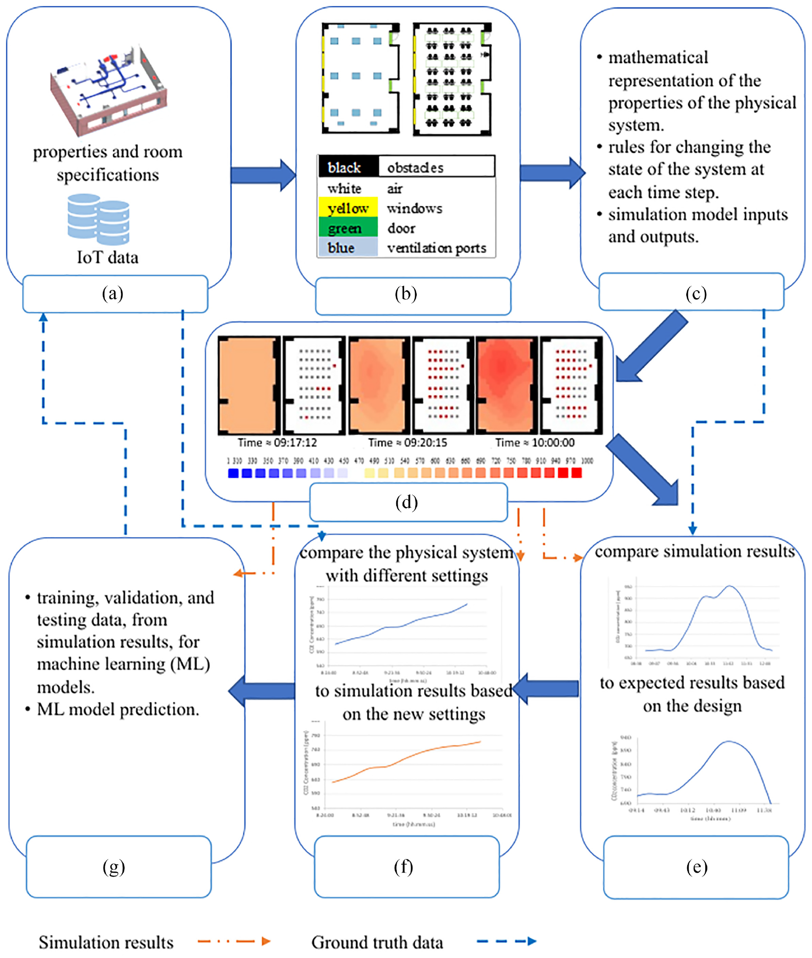
A framework that integrates data collection, M&S process, and machine learning (ML) to predict values of the configuration parameters to improve indoor air quality. (a) Physical system. (b) Conceptual model. (c) Computer model. (d) Simulation results. (e) Simulation model verification. (f) Simulation model validation. (g) ML predictions.

As shown in Figure 1, the cycle of the presented framework starts by collecting CO₂ level data from the physical space with known settings through the CO₂ sensors (Figure 1(a)). Next, a conceptual cellular model (Figure 1(b)) is created based on the known settings of the space (e.g., ambient CO₂ concentration and floorplan). Then, the cellular model rules by which CO₂ levels may change in each area of the space are developed, and those rules are converted into a Cell-DEVS model (simulation model) (Figure 1(c)). In the following step, the Cell-DEVS models are executed to mimic the behavior of the physical system. This step in Figure 1 shows the simulation results at the beginning of the simulation, where only a few occupants are present, and during other timestamps as occupants arrive (Figure 1(d)). At each shown time stamp, CO₂ concentration, and the occupants’ locations are visualized. Verifying the Cell-DEVS model entails testing by comparing the simulation results to the results calculated based on the Cell-DEVS model design and formal definition, as shown in Figure 1(e). Note that if the simulation results are identical to what is expected by the model design, this does not necessarily guarantee the model’s validity. For validity, the simulation results must be compared against the data collected from the physical system. In step (f) of Figure 1, the simulation results are compared to the data collected from IoT devices to ensure they resemble the physical system and validate the quality of the results. In the final step (Figure 1(g)), we integrate ML models that are trained using the simulation results obtained in Figure 1(d) to predict unknown configuration parameters of the modeled space (e.g., location for ventilation ports or computer desk arrangements in a laboratory). The ML integration overcomes the fact that generating, simulating, and studying the simulation of altering the values of the several settings that interact to affect CO₂ levels is very time-consuming. Without the ML prediction step, the designers would need to simulate many possible scenarios with minor alterations to find the optimal settings for better indoor air quality. Building designers can then use the results to choose the best configuration parameters for the physical system. We implement the designed framework using Python scripts and show the application of the framework through a real-life case study. The dataset generated in the case study is publicly available through our repository.⁹

The rest of this paper is organized as follows. In Section 2, we review related work, and in Section 3, we discuss the background needed to present our work. In Section 4, we explain the methodologies and the experimental setup that we have created to perform our study, and that can be used in similar studies. In Section 5, we present a case study to illustrate the models we create, and the framework proposed in Figure 1. Finally, we discuss the research work done, the experimentation, and the results in Section 6.

2. Literature review

Researchers have used M&S and optimization techniques to experiment and observe CO₂ dispersion indoors in different settings. Batog and Badura model a bedroom that contains a bed, a wardrobe, and a single-breathing occupant. They simulate the model in two different scenarios. In the first scenario, CO₂ can escape through gaps around the windows and doors, while in the other scenario, CO₂ is trapped inside the room. The occupant is assumed to spend 8 h sleeping in the room. As a result of the study, the authors recommend considering the thoughtful placement of CO₂ sensors, as the location of the sensors affects the accuracy of the measurements. For example, placing CO₂ sensors in corners near windows or open doors may result in lower readings than the actual CO₂ concentration levels close to where the occupant sleeps. They also recommend that the height at which the sensor is installed should be above the level of the bed.¹⁰ Pantazaras et al. present a method for tailoring models for specific spaces. The models consider the CO₂ concentration, ventilation, and multiple occupants. Their models are used to predict CO₂ concentration levels in the room and are only effective for short-term predictions of CO₂ concentration levels.¹¹ Makmul studies the dispersion of hazardous gases in enclosed spaces to aid building designers in constructing public spaces that are safer during evacuation.¹² The author uses CA to model the influence of the spread of gas on the behavior of pedestrians. In their study, Makmul presents an experiment on a specific closed space model with two exits. The have used model is a 2-D model that does not consider indoor space height.¹²

Zuraimi et al.¹³ use ML methods to predict the number of occupants in enclosed spaces based on CO₂ measures. For their study, they used a large room with a capacity of 200 occupants. In the study, CO₂ measurements and actual number of occupants are collected for 4 months to train the model. The authors prove by experimentation that using ML models improves the accuracy of occupants’ detection over dynamic physical models in detecting the number of occupants based on CO₂ measures. However, this method can only be applied when the settings, such as dimensions and ventilation, are constant while the number of occupants, and hence the CO₂ measurements, changes. Changes in seating arrangements or the number of ventilation ports, for instance, would deem the ML predictions invalid.

Heo et al.¹⁴ propose a deep reinforcement learning algorithm to design the ventilation system in a subway station. The model is trained using synthetic data generated by a virtual gray box model. The gray box model predicts the indoor Particle Matter (PM) based on some variables (e.g., the volume of the subway station and the efficiency of the ventilation filters). The authors state that the virtual model does not properly imitate the real subway station and, hence, the performance of the ML model may not be stable in real-life scenarios. Despite this shortcoming, the study has succeeded in reducing the energy consumption in the subject subway station by adjusting the ventilation based on the predicted PM levels. The method is specific to one subway station that was used to collect data and validate the model as well. As such, the authors suggest enhancing the method to be able to generalize it to other types of buildings.¹⁴

Tagliabue et al. use real-life data collected from CO₂ sensors and feed the data to a recurrent neural network to predict future CO₂ levels in an educational laboratory. The study aims to adjust the Heating, Ventilation, and Air Conditioning (HVAC) based on the predicted CO₂ concentration. Studying the effect of changing any of the settings in the room is not covered in the study.¹⁵ Similar to the previous research, the results can only be applied to the same space where the data was collected with fixed room settings.

Taheri and Razban provide a system to control HVAC based on the CO₂ concentration in the environment. They learned that Artificial Neural Network (ANN) is better than other ML algorithms at predicting CO₂ levels due to the nonlinearity associated with CO₂ data. The CO₂ level estimations were based on university class schedules and fixed assumptions regarding attendance rate. Like Heo et al., the ML model was validated against the same space where the data used to build the model was collected. Thus, the ML model is valid relative to that space setting. Furthermore, any changes in dimensions or seating arrangement are not considered. The study assumes that the number of occupants is constant over a short period and changes over a longer period such as 1 h. They use the ML model to predict the CO₂ levels based on occupancy, relative humidity, dew point, and temperature. The ventilation system is controlled to maintain the required indoor CO₂ levels to achieve a balanced tradeoff between healthy air quality and energy consumption.¹⁶

A more general study, by Ma et al., surveys several research projects developed to study indoor air quality. To understand the effect of variables influencing indoor air quality, the authors review analytical models and consider using the input variables of those models as inputs for ANN and reinforcement learning (RL) model predictions. Based on the review, the authors conclude that a limited number of studies have considered spatial configuration (e.g., room dimensions) to adjust the control systems or to incorporate those factors in predictive models. They also state that, although analytical models consider many factors affecting indoor air quality, no research studies the effect of the combination of those variables using ML. The authors suggest that the lack of large datasets and the difficulty of collecting field measurements could be the reason for the deficiency. They recommend future studies to test variable combinations to develop effective models.¹⁷

Based on our research and the findings of Ma et al., the problem of predicting the combined effect of the different parameters affecting the enclosed space settings on indoor air quality is still pertinent due to the lack of large datasets and the difficulty of collecting ground truth data. Furthermore, the available research does not provide a realistic generic solution that is not specific to one enclosed space.

We address the gaps highlighted by three main contributions. First, contrary to previous research that deals with the problem in a case-by-case manner and considers a small subset of the indoor room settings, we offer a generic Cell-DEVS model of CO₂ dispersion using well-established formalism that is supported by tools. The Cell-DEVS model we present is validated against ground truth data collected from different real university laboratories with occupants and various settings. Therefore, it can be applied to different enclosed spaces. Second, by integrating the Cell-DEVS model, which has been validated and calibrated against real-life data, into a framework to generate scenarios of various enclosed spaces and simulate those scenarios, we provide a large set of valid synthetic data that is otherwise unavailable through physical means. Third, encompassing training an ML algorithm in the framework and training it using the simulation results allows for fast predictions without the need to create scenarios and run simulations for studying the results of tweaking the values of each indoor setting. We choose ML over other methods because it is capable of handling the complex interaction of all the variables influencing CO₂ dispersion as a simple black box without the need to understand or model the details of the underlying physics.

That said, the use of ML is not the main contribution of this research. The main contribution of this research is the complete framework with methodological and verified steps. Those defined steps address the lack of real-life CO₂ measurement data for all various room settings and the difficulty of generating valid synthetic data representing various combinations of room settings that may affect CO₂ levels and dispersion. Building designers and maintainers can use the proposed framework to determine values for unknown parameters or find optimal design configurations for various enclosed spaces.

3. Background

In this section, we describe the essential background for the two methods we use: M&S and ML. We model CO₂ dispersion using Cell-DEVS.¹⁸ Cell-DEVS defines a grid of cells where each cell is specified as a DEVS model. The state of the cell is calculated using a predefined computation function that takes into consideration the current state of that cell and the states of the neighboring cells. The use of neighborhoods and spatial complexity makes CA, and hence Cell-DEVS, inherently suitable for modeling spaces such as rooms and buildings. However, Cell-DEVS is chosen over CA because it overcomes some of the disadvantages of CA in building advanced cellular models.¹⁸ For example, Cell-DEVS supports asynchronous execution of the cells forming the grid and allows for defining complex timing conditions. As such, Cell-DEVS is suitable for modeling complex environmental and social systems and is very applicable to spatial models involving interacting variables.^18,19 Another motivation that explains choosing Cell-DEVS for our framework is the availability of various tools on different platforms that support Cell-DEVS as an M&S method.^19,20

A Cell-DEVS model can be formalized as follows: GCC = (X_list, Y_list, I, X, Y, η, N, {t₁, . . ., t_n}, C, B, Z), where X_list is the list of external input couplings (i.e., input values to the cell that couples it with its defined neighbors), Y_list is the list of external output couplings, I is the set of states, X is the external input events set, Y is the external output events set, η is the neighborhood size, N is the neighborhood set, {t₁, . . ., t_n} is the number of cells in each dimension, C is the cell space, B defines the border cells, and Z is a translation function that defines internal and external coupling.

The second concept we explain in this section is the ML technique we use. We use deep learning to find the optimal configuration parameters for a given space. Deep learning is a type of Neural Network (NN) that is in turn an ML technique inspired by the function of the brain’s neurons. NN analyzes the data by passing it through a hierarchy of layers of interconnected neurons. Deep learning is training an NN that has more than two non-output layers (Figure 2).²¹ As shown in Figure 2, a layer in a Deep Neural Network (DNN) can be either the input layer, a hidden layer, or the output layer. The input layer groups the inputs (x₁, . . ., x_i) and does not perform any computing, while the output layer is the group of neurons that provides the outputs (y₁, . . ., y_j). As for the hidden layers (h₁, . . ., h_k), these are the layers of neurons that perform the actual computing and are not seen by the user. As the data passes through each hidden layer, the data becomes clearer based on the analysis and processing done at each layer until the results are achieved at the output layer.

Figure 2.

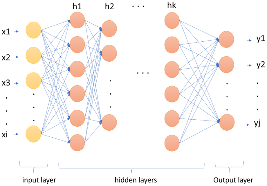
A hierarchy of several layers of neurons is a deep learning network.

For a DNN to perform such a task, it needs to be trained using a labeled data set where the outputs for the given inputs are already known. In this phase, the DNN makes predictions and compares them to the expected outputs. Based on this comparison, the strengths of the connections between the neurons of the different layers are adjusted. This adjustment continues until the DNN becomes able to predict outputs with acceptable accuracy.²¹ Although other ML algorithms may be suggested to replace the DNN in our framework, many considerations must be studied. For example, we choose DNN over RL because DNN is more suitable for the problem we are attempting to solve. RL learns from the data dynamically and adjusts the parameters based on that. When applying this to the CO₂ dispersion problem, the room settings scenario would have to be adjusted and a new simulation would have to be executed before the RL continues the prediction and learning process. The building designer using the framework would spend more time in the prediction process than required. On the contrary, in the proposed framework, all the scenarios are generated and simulated in advance before running the DNN and starting the prediction process. This allows for quicker predictions, given the data is available. However, we plan to investigate replacing the DNN with other ML algorithms or Genetic Algorithms (GA) in future work.

4. Methodology and experimental setup

For the simulation model presented in this paper, we use the Cadmium Cell-DEVS simulator.²⁰ Cadmium is a cross-platform header-only C++ library that can be used to implement and simulate Cell-DEVS models. The simulator allows defining a general category of models using the programming language (C++) while reading specific configuration details for each model from a JavaScript Object Notation (JSON) file that is parsed by the simulator. On the one hand, we have implemented one general model in C++ for CO₂ dispersion and the breathing of occupants. On the other hand, the JSON file describes different initial configurations per cell. Each cell represents a specific segment of the physical space. The JSON file also specifies the dimensions of the room, the shape of the cells’ neighborhood, and other configuration parameters. For visualizing the simulation results, we use Advanced Real-time Simulation Laboratory (ARSLab) DEVSWeb Viewer.²²

The general model we are presenting considers the dimensions of the closed space, ambient CO₂ concentration, size, and location of CO₂ sinks (i.e., windows, doors, and ventilation ports), locations where occupants may exist, the breathing rate of occupants based on their activity level, concentration increase due to breathing occupants, and dimensions of the room. The model assumes an ambient outdoor CO₂ concentration of 400 particles per million (ppm) based on the American Society of Heating, Refrigerating, and Air-Conditioning Engineers (ASHRAE) standards.²³ However, this value can be adjusted as a parameter specified for each JSON scenario. Human breathing is calculated based on the fact that humans breathe every 5 s, and the produced CO₂ in every breath (exhaling and inhaling) is a parameter that depends on the activity level.²⁴

To convert the conceptual model to a Cell-DEVS computer model, the details of the enclosed space are translated into cells of different types. The general model has eight types of cells: (1) walls and obstacles that do not allow CO₂ diffusion, (2) air cells whose CO₂ concentration is dependent on the concentration values in their neighborhoods, (3) CO₂ sources with a periodic increase in the CO₂ level added at an interval to mimic breathing in addition to the CO₂ diffused from the neighborhood, (4) open doors that diffuse CO₂ to the rest of the building with a fixed indoor background CO₂ level, (5) open windows that are also CO₂ sinks with a fixed outdoor background CO₂, (6) vents that diffuse gas through HVAC system with a reduced constant CO₂ level, (7) workstation cells that act as normal air cells when not occupied and as CO₂ sources when occupied, and (8) exposed occupants cell that represents occupants who have been exposed to air with high CO₂ concentration for a long period and thus they are at risk of infection or other health issues. The CO₂ diffusion is calculated by averaging the concentration level in the Moore neighborhood of each cell. This means that to get the concentration of each cell, the concentrations in either 27 or 9 cells are averaged in the cases of 3-D and 2-D models, respectively.

We illustrate the ML portion of the proposed framework including the data generation, ML model training, and using the prediction model in Figure 3. We have implemented a group of Python classes as a toolchain to generate and simulate multiple scenarios of the model of the physical space being studied.

Figure 3.

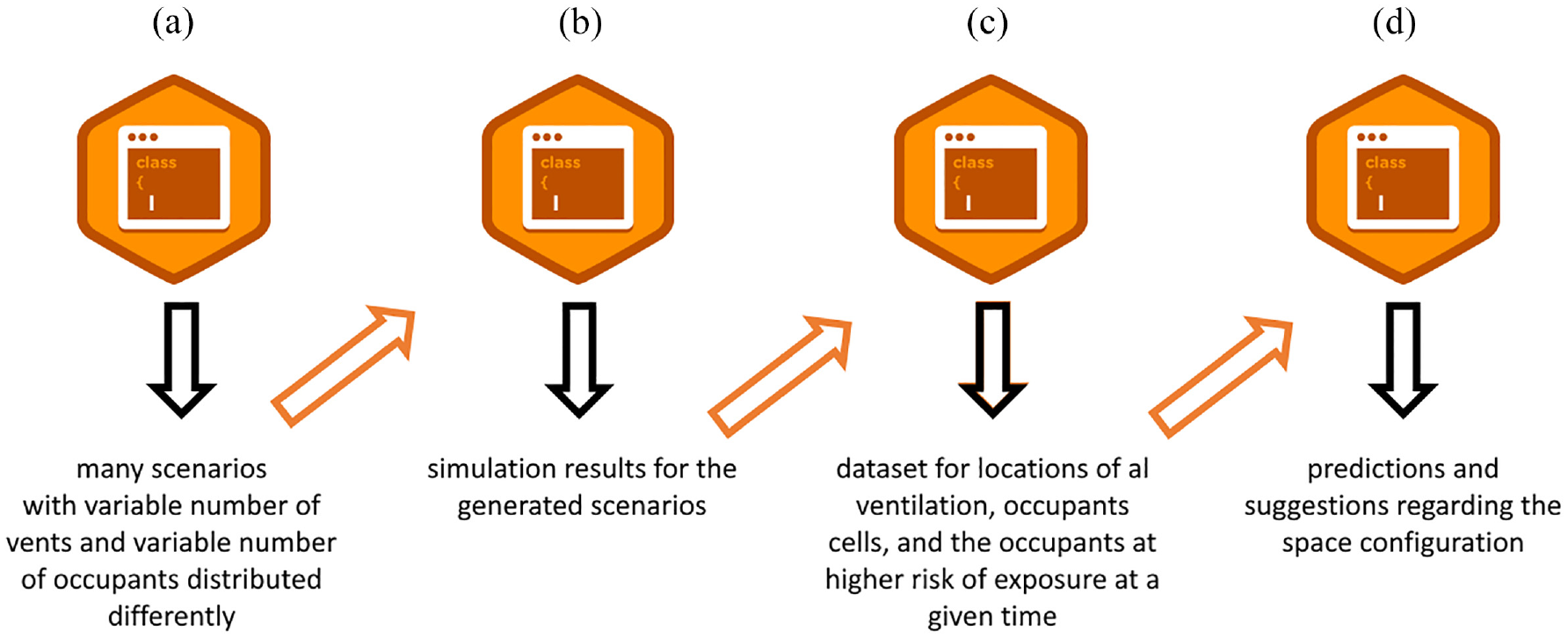
The experimental setup used to implement the framework is presented in Figure 1. (a) Generator. (b) Simulator. (c) DataCollector. (d) Predictor.

The process starts with the Generator class (Figure 3(a)) that takes an initial scenario, the number of vents, vent size, and the number of occupants in the modeled space as inputs. The generator then creates many variations (JSON files) of that scenario with random values (drawn from a uniform distribution) of the configuration parameters. The parameters considered can be changed in other experiments using the same experimental setup. The Simulator (Figure 3(b)) calls Cadmium to simulate all the generated scenarios produced by the generator. The log files resulting from the simulator are locally stored. In the following step, the DataCollector (Figure 3(c)) parses the log files to collect data about where the generated vents are located, the locations of occupants, and the number of occupants who become exposed to air with high CO₂ concentration at a given point during the simulation. The DataCollector produces a Comma-Separated Values (CSV) file that contains all the required information from the simulation results of all scenarios. The final step is the Predictor (Figure 3(d)), which in turn uses the CSV file generated by the DataCollector as a labeled dataset to train a DNN model. Some of the configuration parameters are chosen as input features to the DNN to predict unknown parameters. The choice of the input features and the predicted output vary depending on the objective of the case study.

For implementing the DNN, we use Keras which is an NN Python library that runs on top of the open-source platform TensorFlow.²⁵ Usually, the more layers the DNN has, the better its ability to learn, but the slower the training is and the more challenging the model becomes due to possible overfitting (giving accurate predictions for the training data but not for the new data). Many researchers provide guidelines for determining the network topology (e.g., the number of hidden layers) based on the number of inputs, the number of outputs, and the nature of the problem, while others recommend a more elaborate approach for determining the network topology for complex problems. Based on theoretical guidelines provided in the literature,²⁶ we started with two hidden layers and manually experimented with changing the number of layers and the number of neurons in the hidden layers. The best results we achieved for the problem at hand were by using two hidden layers where each layer has 20 nodes. To cross-validate the machine learning model, we use the k-fold statistical resampling to evaluate the prediction accuracy of the model. The k in “k-fold” refers to the number of groups that the data is to be split into. The dataset is shuffled randomly and divided into k groups. For each group i, we use the remaining k−1 groups as a training data set while group i is used as a testing dataset to evaluate the model. We use 10-fold cross-validation for our dataset. In other words, in each fold, 90% of the data is used for training while 10% is used for validation and the process is then repeated 10 times.

5. Case study: predicting number of sick occupants based on vents locations, number of vents, and the total number of occupants

In this section, we present a case study that covers the framework, starting by creating a conceptual model from the physical system and ending with the ML prediction of some room settings.

5.1. From the physical system to the computer model

The computer laboratory we use in this case study for data collection and verification is a (9.5×14.24×3.25) m³ room, with 48 workstations where students can sit to work on their computer assignments. The floor plan of the laboratory and the furniture layout are shown in Figure 4. The ground truth data, collected from CO₂ sensors installed in a university laboratory, is based on the number of attendees for a 110-min tutorial that has taken place in the Winter term of the year 2019. Thirty-nine students attended the tutorial, in addition to the teaching assistant who was present throughout the tutorial. Students arrive and leave at different times during the period of the lab tutorial.

Figure 4.

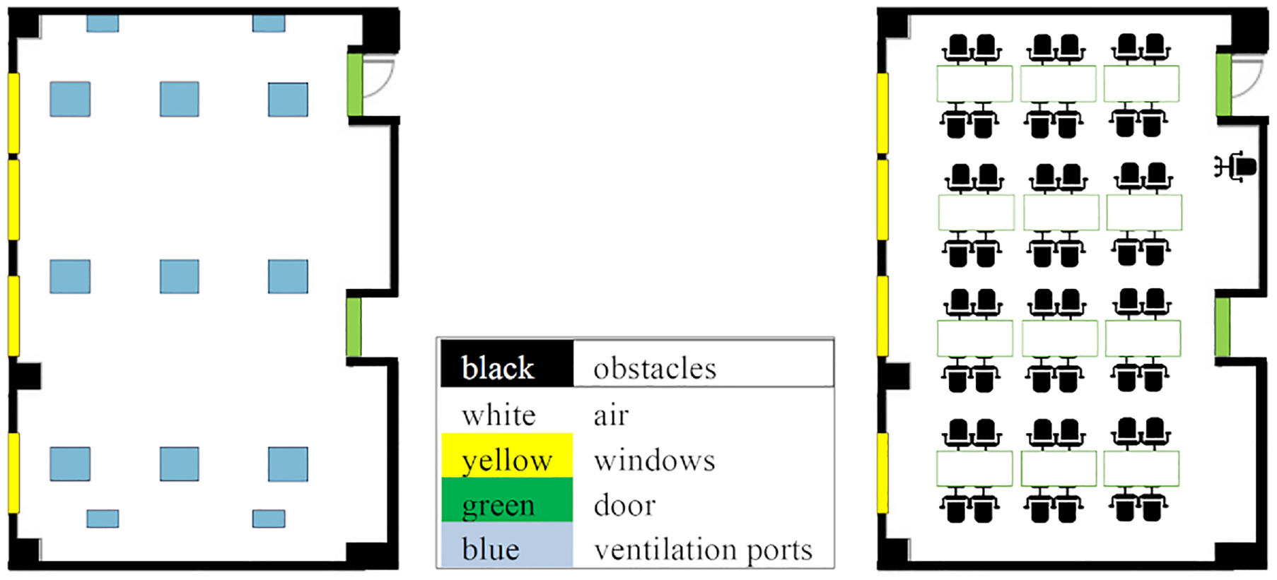
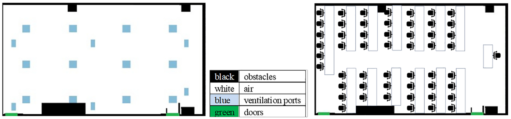
Approximate floorplan (left) and furniture layout (right) of the physical system of the calibration model.

The logged data against which the Cell_DEVS model in Figure 5 is validated is based on one CO₂ sensor installed close to the door at 1.5 m height and logs the concentration level every 30 min. As the occupants arrive at the room, the readings of CO₂ concentration start to increase, reaching the peak after the middle of the lab tutorial period when all students are present. The CO₂ starts to decrease again until all students leave the room. In Figure 5, snapshots of the simulation show the increase in CO₂ as the occupants arrive. The simulation video shows a longer coverage of the CO₂ dispersion including the decrease in CO₂ as the occupants leave the room.²⁷

Figure 5.

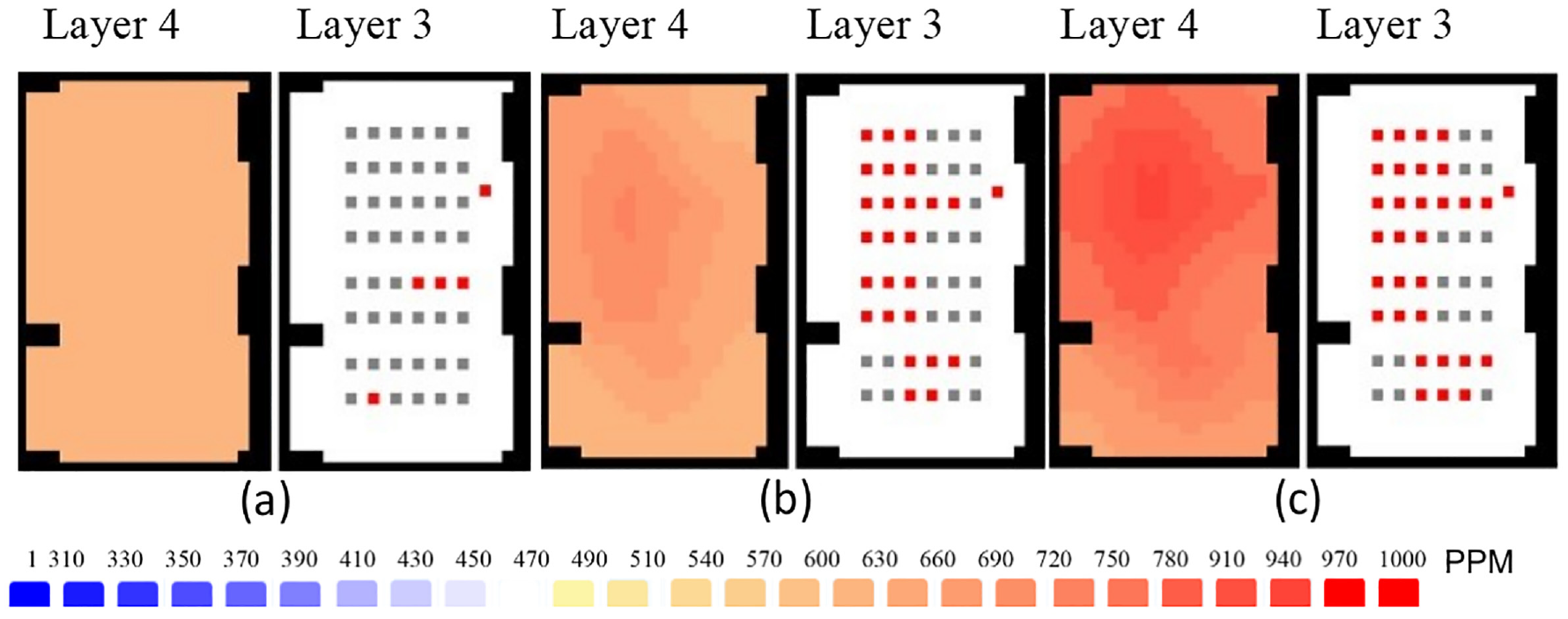
Simulation results during different timestamps (hh:mm:ss). The legend in the figure illustrates the color code of the CO₂ levels in PPM in Layer 4. The red squares in Layer 3 represent occupants, while the gray squares are empty workstations. (a) Time ≈ 09:17:12. (b) Time ≈ 09:20:15. (c) Time ≈ 10:00:00.

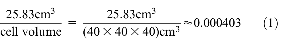
Note that we have created two versions of this model: a 3-D detailed version and another 2-D version. Both versions are calibrated separately based on the real-life data collected from the university laboratory physical system. We explain here the detailed 3-D version of the model and the reader is referred to previous publications for more details about the 2-D version.²⁴ The physical 9.5 × 14.24 × 3.25 m³ system is mapped to a 23×35×8 cell³ Cell_DEVS model. For this case study, we specify a 40 × 40 × 40 cm³ cell size. Therefore, the physical system is translated to an approximated (23 × 35 × 8) cell model. To replicate the physical system, the CO₂ production for each occupant is calculated as follows based on two facts: (1) an average-sized person doing normal low-activity office work produces 0.31 liter/min/person of CO₂₂²³ and (2) breathing occurs every 5 s on average. Therefore, an average person produces 0.02583×1000 cm³ of CO₂ per breath. Hence, every occupant’s breath increases the concentration of CO₂ in each occupied cell by:

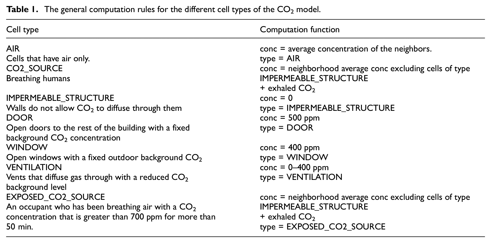
\frac{25.83 c m^{3}}{cell volume} = \frac{25.83 c m^{3}}{(40 \times 40 \times 40) c m^{3}} \approx 0.000403

(1)

It is worth noting that Equation (1) gets calculated automatically based on the Cell_DEVS model parameters (i.e., cell volume and produced CO₂ per breath specified in the input JSON settings file). We include here how this calculation is done for the parameters we specify for the presented case study. The general computation rules for the different cell types are shown in Table 1. Note that the workstation cell type is not listed in Table 1 because it either behaves as a CO₂_SOURCE (when occupied) or as an AIR cell when not occupied. It is not considered as an IMPERMEABLE_STRUCTURE because we assume that the type of workstations in this room occupies minimum space that does not affect CO₂ dispersion. The Cell_DEVS model formalism is specified as follows: CO₂ = <X_list, Y_list, Z_list, S, X, Y, Z, η, N, {t₁, t₂, t₃}, C, B, Z>, where X_list = Y_list = Z_list = {Ø}; S = type: {0, 1, 2, 3, 4, 5, 6} and conc: {double}; X = Y = Z = Ø; η = 27; N = (0,0,0), (−1,0,0), (1,0,0), (0,1,0), (0,−1,0), (−1,1,0), (1,1,0), (−1,−1,0), (1,−1,0), (0,0,1), (−1,0,1), (1,0,1), (0,1,1), (0,−1,1), (−1,1,1), (1,1,1), (−1,−1,1), (1,−1,1), (0,0,−1), (−1,0,−1), (1,0,−1), (0,1,−1), (0,−1,−1), (−1,1,−1), (1,1,−1), (−1,−1,−1), (1,−1,−1)}; t₁ = 23; t₂ = 35; t₃ = 8; C = {C_ijk—i ∈ (0, 23[ ^ j ∈ [0, 35[ ^ k ∈ [0, 8[ }; and B = {Ø} (unwrapped cell space).

Table 1.

The general computation rules for the different cell types of the CO₂ model.

Cell type	Computation function
AIR Cells that have air only.	conc = average concentration of the neighbors. type = AIR
CO2_SOURCE Breathing humans	conc = neighborhood average conc excluding cells of type IMPERMEABLE_STRUCTURE + exhaled CO₂
IMPERMEABLE_STRUCTURE Walls do not allow CO₂ to diffuse through them	conc = 0 type = IMPERMEABLE_STRUCTURE
DOOR Open doors to the rest of the building with a fixed background CO₂ concentration	conc = 500 ppm type = DOOR
WINDOW Open windows with a fixed outdoor background CO₂	conc = 400 ppm type = WINDOW
VENTILATION Vents that diffuse gas through with a reduced CO₂ background level	conc = 0–400 ppm type = VENTILATION
EXPOSED_CO2_SOURCE An occupant who has been breathing air with a CO₂ concentration that is greater than 700 ppm for more than 50 min.	conc = neighborhood average conc excluding cells of type IMPERMEABLE_STRUCTURE + exhaled CO₂ type = EXPOSED_CO2_SOURCE

The simulation runs 7200 timesteps which are equivalent to 2 h; each time step is 1 s. The session lasted for 110 min and we added 5 min before and after the session to get a better picture of the CO₂ level changes due to the arrival and departure of occupants. Figure 5(a) shows the simulation results at the beginning of the simulation, where only a few occupants are present, and during other timestamps, as occupants start to arrive (Figure 5(b) and (c)). CO₂ concentration is to the left of each figure (a, b, and c) and the occupants’ locations are at the right. Occupants are represented as red squares and empty workstations are gray. The two grids repeated three times in three timestamps in the Figure are Layer 4 (left), which is the cross-section of the room representing the height at which the CO₂ sensor is installed (120–160 cm), and Layer 3 (right) representing the height at which the occupants are seated (80–120 cm). The area in the lower left corner of the room has fewer occupants and is close to the vents (the locations of the vents are shown in Figure 4). Hence, it has less CO₂ concentration than other areas, as the vents try to offset the CO₂ increase that occurs where the occupants are concentrated. Note that Layer 3 in Figure 4 displays only the workstations, and not the CO₂ concentration, as the purpose of displaying Layer 3 here is to show the potential locations of the occupants.

5.2. Model calibration, verification, and validation

The general model has flexible parameters, some of which are not available in the set of ground truth data that we have collected. For example, although the exact number of attendees in the lab is available, the arrival time of each person at the computer workstation they have used is not available. Also, the exact CO₂ concentration in the vents is not available. Thus, we have adjusted the values of the unknown parameters through several simulation experiments to calibrate the model to get simulation results that are as close as possible to the ground truth data. The parameters that we adjusted are the arrival and departure times of the occupants, the workstations that the occupants chose to use, ambient CO₂ concentration, and CO₂ concentration in the air bumped into the room through the ventilation ports. We have documented the exact steps to execute the model and made it available with the code and the different scenarios through the ARSLab repository.⁶

After calibrating the model by adjusting the initial parameters (e.g., initial CO₂ concentration level) using the ground truth data, we validate the rules used in the presented CO₂ Cell_DEVS model using another room in the same building but on a different floor and with a different configuration. The physical system used for validation is another laboratory setting during a different time of the day, with only 11 occupants, a larger space, and no windows. While we create, calibrate, and verify the Cell-DEVS model using settings and ground truth data collected from the first laboratory explained in section 5.1, we validate the Cell-DEVS model using ground truth data collected from a different laboratory with different settings. This methodology increases the trust in the synthetic data generated by simulating different scenarios with various room settings. Furthermore, it allows for the use of the generated data in training the ML for the prediction step of the proposed framework. The dimensions of the physical system used for validation are 15.8 × 9 × 3.25 m³. Figure 6 shows the floor plan of the room and the furniture layout. In this room, there is another lab session following this one, and hence more students enter the room at the end of the laboratory, and we have tried to mimic this in the model. The CO₂ sensor is installed close to the door and logs the concentration level every 15 min.

Figure 6.

Floor plan and furniture layout of the validation model.

The formal Cell_DEVS scenario for the validation room is similar to the formal calibration Cell_DEVS scenario explained for the room where the data was collected except for the following: t₁ = 23; t₂ = 40; and C = {C_ijk—i ∈ (0, 23[ ^ j ∈ [0, 40[ ^ k ∈ [0, 8[}. We have used the same ambient CO₂ concentration and ventilation concentration that have resulted from calibrating the Cell_DEVS model. We have executed the Cell_DEVS model for a simulation period equivalent to 7200 s (2 h). Comparing the simulation results to the data logged by the real sensors in the physical system (Figure 7) demonstrates the resemblance between the model’s data and the system’s data. Simulation videos of the validation model and the original CO₂ model are available online through the ARSLab YouTube channel.²⁷

Figure 7.

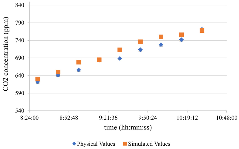
Collected ground truth data points in the validation model compared to simulation data.

5.3. ML prediction examples

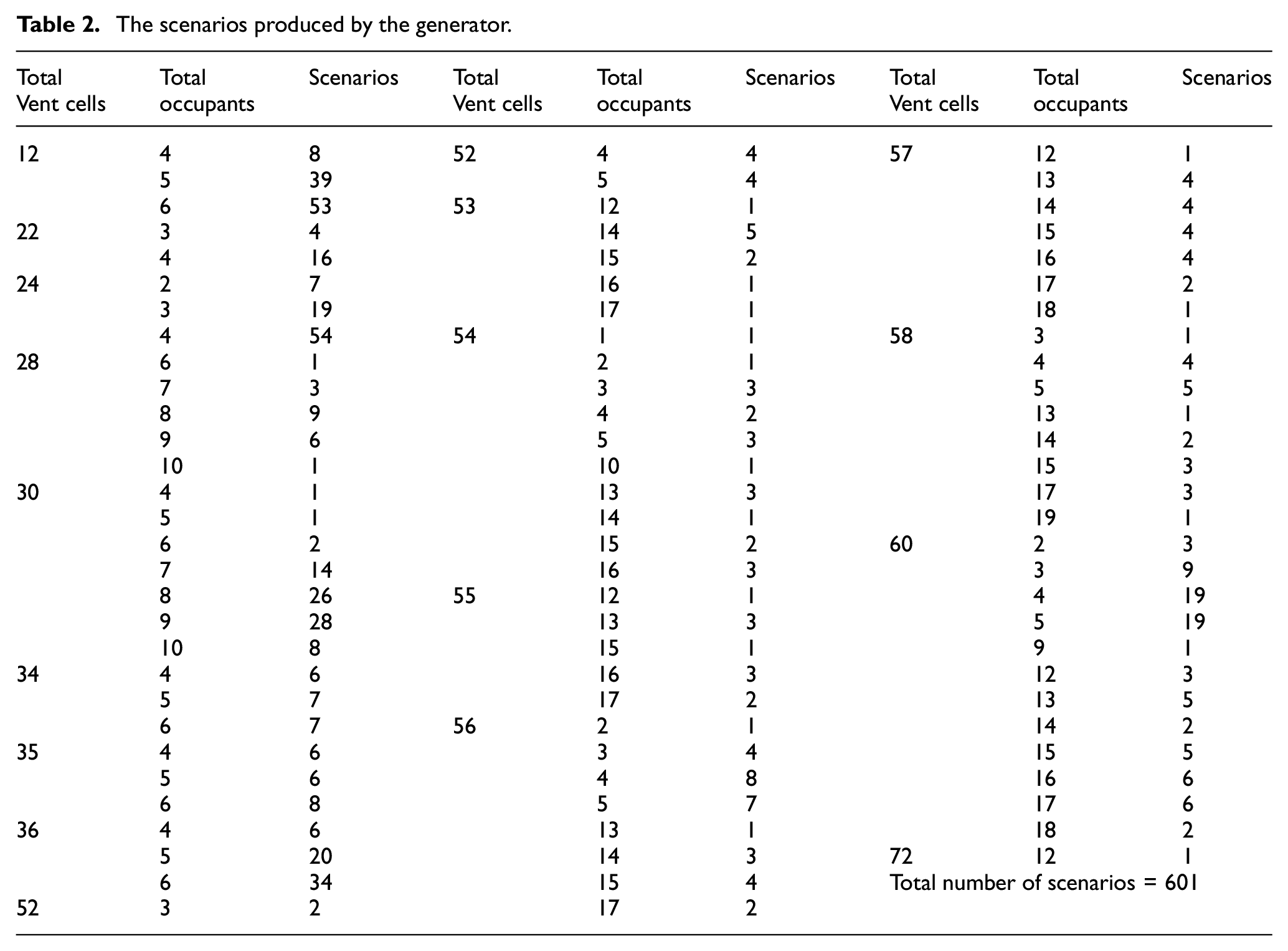
For the ML prediction example included in this study, we use the 2-D version of the model that has also been calibrated against real-life data. While we chose the 2-D version to reduce execution time for this case study, applying the ML prediction to the 3-D version of the model will be presented in future studies. We have used the framework to automatically generate around 600 scenarios with different settings of the Cell_DEVS model using the Generator (Figure 3(a)). The input features to the DNN in this case study are the locations of the vents, the number of vents, and the total number of occupants in the room. The output of the DNN is the location and the number of occupants exposed to high CO₂ concentration by the end of the session. Table 2 lists the generated scenarios, the number of cells of type VENTILATION, and the number of occupants (CO2_SOURCE) generated for those scenarios. Note that a ventilation port is composed of several cells. For example, the sample simulation shown in Figure 8 has ventilation ports composed of 6 (2 × 3) cells each. For this case study, When the number of sick occupants is known for each scenario (design of ventilation ports and their locations), it is easy to decide which ventilation ports’ locations are the most suitable or what the maximum number of occupants should be in a room with certain settings. It is important to state that while we present this case study for illustration, the same framework supports testing the effect of other settings of the closed space on the CO₂ concentration or occupants’ health. For example, if the dimensions are the settings to be altered and tested to enhance the room design, the width, length, and heights would be added as features when training the DNN model.

Table 2.

The scenarios produced by the generator.

Total Vent cells	Total occupants	Scenarios	Total Vent cells	Total occupants	Scenarios	Total Vent cells	Total occupants	Scenarios
12	4	8	52	4	4	57	12	1
	5	39	52	5	4		13	4
	6	53	53	12	1		14	4
22	3	4		14	5		15	4
22	4	16		15	2		16	4
24	2	7		16	1		17	2
	3	19		17	1		18	1
	4	54	54	1	1	58	3	1
28	6	1		2	1		4	4
	7	3		3	3		5	5
	8	9		4	2		13	1
	9	6		5	3		14	2
	10	1		10	1		15	3
30	4	1		13	3		17	3
	5	1		14	1		19	1
	6	2		15	2	60	2	3
	7	14		16	3		3	9
	8	26	55	12	1		4	19
	9	28		13	3		5	19
	10	8		15	1		9	1
34	4	6		16	3		12	3
	5	7		17	2		13	5
	6	7	56	2	1		14	2
35	4	6		3	4		15	5
	5	6		4	8		16	6
	6	8		5	7		17	6
36	4	6		13	1		18	2
	5	20		14	3	72	12	1
	6	34		15	4	Total number of scenarios = 601
52	3	2		17	2	Total number of scenarios = 601

Figure 8.

An automatically generated and simulated scenario using the setup of Figure 3. The legend in the figure illustrates the color code of the CO₂ levels in PPM in Layer 4. The scenario maps to the room in Figure 4. (a) Time ≈ 0. (b) Time ≈ 1 h.

When validating the DNN model, we use 10-k cross-validation. In each fold, the data is split into 540 training scenarios and around 60 validation scenarios to test the predictions of the DNN when given new input.

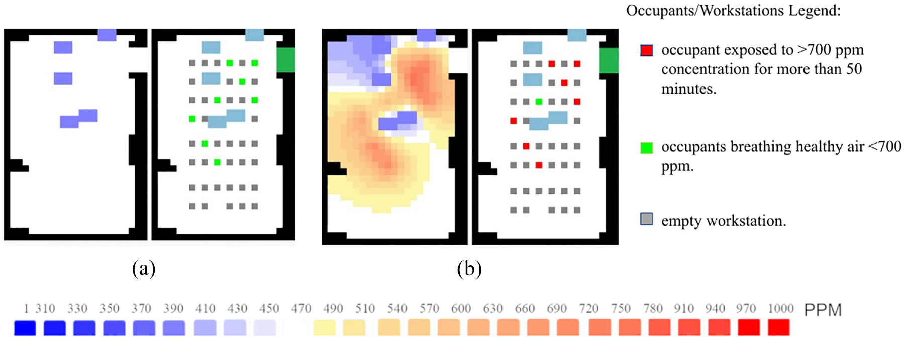
We simulate all the scenarios and collect the data using the DataCollector (Figure 3(c)). It is worth noting that the simulation time is highly dependent on the scenario size and granularity. For this case study, the 2-D version of the Cell-DEVS model generation and simulation takes approximately 3 s on average, on an i7-1165G7 2.80 GHz processor and 12.0 GB RAM. However, generating and simulating many scenarios with different settings is a time-consuming task, given the large number of possible scenarios. For this case, the enclosed space settings used as input features to the DNN are the vents’ dimensions, vents’ coordinates, and the number of occupants. The DataCollector also counts the number of occupants who are specifically surrounded by higher CO₂ concentrations (hence bad air quality) for a longer period (EXPOSED_CO₂_SOURCE). The latter is the data label, which will be predicted by the DNN model once trained and validated. Based on the predicted values, the settings of the room can be adjusted by the designer to meet the air quality requirements of the room. All the generated scenarios and the collected data are available through our repository.⁹ Figure 8 is a snapshot of the simulation for one of the scenarios generated and input to the DNN for training. The scenario has a total of 30 cells of type VENTILATION and a total of 8 occupants. Seven out of the eight occupants are breathing bad air quality after an hour of being in the closed space (Figure 8(b)).

The trained DNN model managed to predict the output (number of occupants exposed to bad air quality) with a mean absolute error of 0.79. We have used the trained and validated DNN to predict the number of occupants for several examples of scenarios with different ventilation ports’ locations, occupancy density, and locations of occupants. For example, we use the DNN to predict the number of sick occupants of the scenario in Figure 9 without simulating the scenario. The DNN predicted the number of occupants exposed to high CO₂ concentration to be 5.69. Then, we simulate the scenario to verify the prediction. The simulation results show that close to the end of the simulation, the number of sick occupants reaches 5, and it remains 5 until the end of the simulation.

Figure 9.

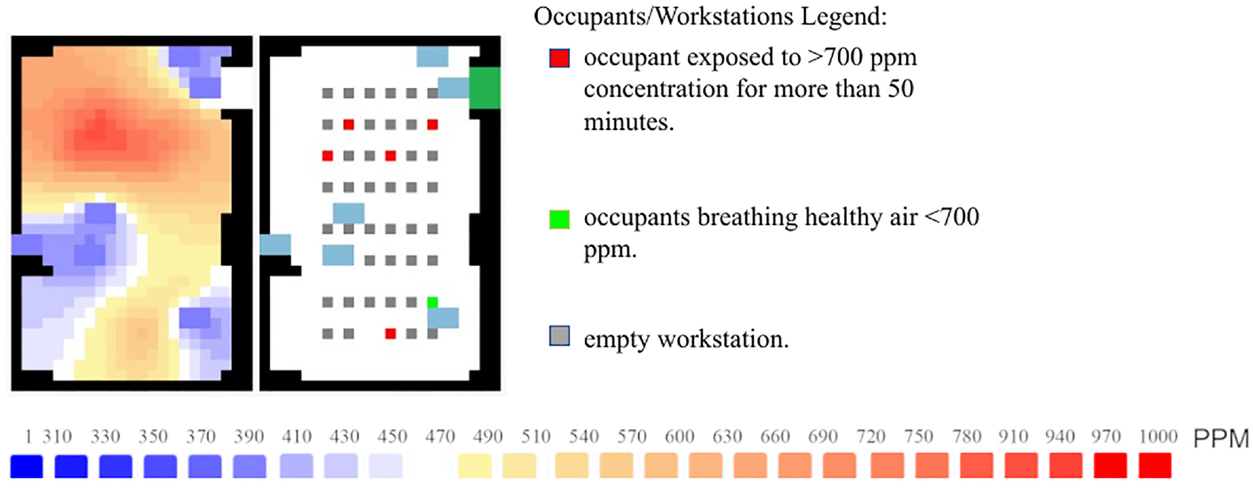
An example of a simulation model where the simulation results in five occupants being exposed to high CO₂ levels, while the DDN model predicts an output of 5.69. The legend in the figure illustrates the color code of the CO₂ levels in PPM in Layer 4. The scenario maps to the room in Figure 4.

6. Discussion and conclusion

Motivated by the need to study the effects of room settings on recorded CO₂ concentration, we have developed a generic Cell-DEVS model that accepts different room settings as input parameters. Then, we validated the Cell_DEVS model using data collected from another closed space in the same building during a different time and with different configurations. When comparing the simulation results to the data collected from IoT devices, the Cell_DEVS model is evinced successful at replicating the behavior of the physical indoor space. In this paper, we integrate the Cell_DEVS model into a novel framework to predict unknown settings of the input space. The framework is composed of several steps: (a) collecting data from physical systems, (b) creating a conceptual model of the collected data, (c) creating a corresponding computer model using Cell-DEVS, (d) simulating scenarios of the created Cell_DEVS model, (e) verifying the simulation results by comparing them to physically measured CO₂ levels, (f) validating the created Cell_DEVS model by comparing results of simulating other variations of that model to data collected from the physical system, and (g) generating a dataset from simulation results to train DNN models for predicting the desired values for settings of enclosed spaces to find optimal designs to enhance air quality. We have illustrated the usability of the framework through a case study where we have generated hundreds of simulation scenarios and used the simulation results to train and validate a DNN model.

The results suggest that the framework is suitable for studying the spread of CO₂ indoors and a presented case study shows that it is successful at predicting variables such as the number of occupants exposed to high CO₂ concentrations for a long time due to inadequate ventilation or misplacements of occupants’ seating. However, as in any other experimental study, some threats to validity are worthy of discussion. A minor validity threat is the existence of some approximations, that do not exceed 20 cm along each dimension when converting the physical system into a model. Nevertheless, this approximation does not affect the usability of the model as the model user is aware of it and can handle slight approximations if needed. A second validity threat is that the current model assumes that the air in the room is at a steady state and the CO₂ is diffused evenly in all directions. This is not usually the case due to the different types of HVAC and occupants breathing in different directions. Incorporating airflow in the room is a feature that we have implemented in the 2-D version of the model,²⁴ and we aim to include it in the 3-D version and the complete framework in future work. However, the model in its current state has successfully mimicked the physical system. Moreover, using more advanced fluid dynamics equations to model the CO₂ dispersion is anticipated to enhance the validity of the results in future work while increasing the simulation time. Other possible future work includes considering occupants’ motion for modeling more dynamic environments (e.g., gymnasiums). Moreover, the ground truth data collected for this study is from two physical spaces. Future studies will increase the trust in the model by collecting data from more physical spaces and comparing the collected data to the model results. Finally, we plan to run experiments to replace the DNN with other methods (e.g., GAs) and target testing and predicting other room settings that may result in better air quality (e.g., furniture layout and ventilation power).

Footnotes

Funding

This work has been partially funded by NSERC (Canada).

ORCID iDs

Hoda Khalil

Gabriel Wainer

Author biographies

Hoda Khalil received her PhD degree from Carleton University. She is an adjunct research professor at the Systems and Computer Engineering Department at Carleton University. Her current research interests are data science, modeling and simulation, and software engineering. Her email is hoda.khalil@carleton.ca.

Gabriel Wainer received his PhD degree from the Universidad de Buenos Aires and IUSPIM (now Polytech de Marseille), Université Aix Marseille (France). He is a full professor at Carleton University. His current research interests are related to modeling methodologies and tools, parallel/distributed simulation, and real-time systems. His email is gwainer@sce.carleton.ca.

References

Al Horr

Arif

Katafygiotoua

, et al. Impact of indoor environmental quality on occupant well-being and comfort: a review of the literature. Int J Sustain Built Environ 2016; 5: 1–11.

Jiang

Masooda

Soh

, et al. Indoor occupancy estimation from carbon dioxide concentration. Energy Build 2016; 131: 132–141.

Labeodan

Zeiler

Boxem

, et al. Occupancy measurement in commercial office buildings for demand-driven control applications—a survey and detection system evaluation. Energy Build 2015; 93: 303–314.

Arief-Ang

Hamilton

Salim

. RUP: large room utilization prediction with carbon dioxide sensor. Pervasive Mob Comput 2918; 46: 49–72.

Wainer

Discrete-event modeling and simulation: a practitioner’s approach. 1st ed. Boca Raton, FL: CRC Press, 2009.

Khalil

Wainer

. CO₂ spread computer lab model user manual, https://github.com/SimulationEverywhere-Models/Cell-DEVS-_spread_indoor/blob/master/User%20Manual.txt

Khalil

Wainer

Dunnigan

. Cell-DEVS models for CO₂ sensors locations in closed spaces. In: Proceedings of 2020 winter simulation conference (WSC), Virtual, 14–18 December 2020.

Khalil

Wainer

Modeling carbon dioxide dispersion indoors: a Cell-DEVS experiment. In: Gwizdałła

Manzoni

Sirakoulis

, et al. (eds) Cellular automata. Cham: Springer, 2021, pp. 226–236.

Khalil

Wainer

. Cell-DEVS-CO₂_spread_indoor, https://github.com/SimulationEverywhere-Models/Cell-DEVS-CO2_spread_indoor/tree/master/scripts/Cell-DEVS_DNN

10.

Batog

Badura

Dynamic of changes in carbon dioxide concentration in bedrooms. Proced Eng 2013; 57: 175–182.

11.

Pantazaras

Lee

Santamouris

, et al. Predicting the CO₂ levels in buildings using deterministic and identified models. Energy Build 2016; 127: 774–785.

12.

Makmul

Microscopic and macroscopic for pedestrian crowds. PhD Thesis, Mannheim University, Mannheim, 2016.

13.

Zuraimi

Pantazaras

Chaturvedi

, et al. Predicting occupancy counts using physical and statistical CO₂-based modeling methodologies. Build Environ 2017; 123: 517–528.

14.

Heo

Nam

Loy-Benitez

, et al. A deep reinforcement learning-based autonomous ventilation control system for SMART indoor air quality management in a subway station. Energy Build 2019; 202: 109440.

15.

Tagliabue

Re Cecconi

Rinaldi

, et al. Data driven indoor air quality prediction in educational facilities based on IOT network. Energy Build 2021; 236: 110782.

16.

Taheri

Razban

Learning-based CO₂ concentration prediction: application to indoor air quality control using demand-controlled ventilation. Build Environ 2021; 205: 108164.

17.

Aviv

Guo

, et al. Measuring the right factors: a review of variables and models for thermal comfort and indoor air quality. Renew Sustain Energ Rev 2021; 135: 110436.

18.

Wainer

Giambiasi

Cell-DEVS/GDEVS for complex continuous systems. Simulation 2005; 81: 137–151.

19.

Khalil

Wainer

Cell-DEVS for social phenomena modeling. IEEE Trans Comput Soc Syst 2020; 7: 725–740.

20.

López

Wainer

Improved cell-DEVS model definition in CD++. In: Sloot

PMA

Chopard

Hoekstra

(eds) Cellular automata. Berlin: Springer, 2004, pp. 803–812.

21.

Burkov

The hundred-page machine learning book. Quebec City, QC, Canada: Andriy Burkov, 2019.

22.

St-Aubin

Wainer

ARSLab DEVS web viewer. Ottawa, ON, Canada: Carleton University, 2020.

23.

ASHRAE Technology Council. Ventilation for acceptable indoor air quality, https://www.ashrae.org/file%20library/technical%20resources/standards%20and%20guidelines/standards%20addenda/62_1_2013_p_20150707.pdf

24.

Altamimi

Khalil

Rajus

, et al. Cell-DEVS models with BIM integration for airborne transmission of COVID-19 indoors. In: Proceedings of the symposium on simulation for architecture and urban design (SIMAUD), Virtual, 14–17 April 2021.

25.

Keras, https://keras.io/

26.

Ibnu

Santoso

Surendro

. Determining the neural network topology. In: Proceedings of the 2019 8th international conference on software and computer applications, Penang, Malaysia, 19–21 February 2019.

27.

ARSLab YouTube. Ottawa: Carleton University; [cited 2023Oct 12]. Available from:. https://www.youtube.com/watch?v=vD7fB2A5hNY, last accessed 2021/11/14

A framework for modeling,generating,simulating,and predicting carbon dioxide dispersion indoors using cell-DEVS and deep learning

Abstract

Keywords

1. Introduction

2. Literature review

3. Background

4. Methodology and experimental setup

5. Case study: predicting number of sick occupants based on vents locations, number of vents, and the total number of occupants

5.1. From the physical system to the computer model

5.2. Model calibration, verification, and validation

5.3. ML prediction examples

6. Discussion and conclusion

Footnotes

Funding

ORCID iDs

Author biographies

References