
Abstract
Simple and computationally efficient drill string models running real-time describing motion in all axes in directional wells are important for the implementation of closed-loop control and assisted monitoring during drilling operations. This paper proposes a new simplified three-dimensional model based on a parametric curve and lumped-parameter modeling, where Kane’s method is used to establish the equations of motion. Validation of the steady-state motion and convergence for the lumped model in vertical and horizontal alignment was compared with a finite-element model. The configuration and restoring forces show good results compared with finite-element analysis. Hence, the model demonstrate the axial contraction as a function of the body restoring forces being oriented to the inertial frame, inherently producing nonlinear coupled axial tension forces. The qualitative response of the model is confirmed in simulation case studies, being showcased by a deviated J-well configuration. Traveling block velocity and top drive torque are included as actuated inputs to analyze off-bottom friction and contact along the wellbore. The model is proposed to act as a virtual sensor for drilling directional wells.
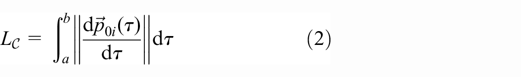
1. Introduction
Thin hydrocarbon reservoir zones require drilling of complex directional wells, including long horizontal lengths for the well to be economically feasible. On the Norwegian Continental Shelf (NCS), several of the oil & gas zones are classified as thin (22–25 m 1 ). Advanced directional drilling methods have been applied to increase oil and gas recovery from these fields on the NCS, such as the Troll and Oseberg field. 2
Oil & gas wells drilled at an angle from the straight vertical geometry are commonly denoted deviated wells. These wells can be preceded with multiple directional changes, including horizontal sections to reach challenging reservoir targets for maximizing hydrocarbon fluid entry into the production well. However, challenges with regards to drilling directional wells are factors such as substantial friction from drill string interacting with the wellbore wall during translatory motion and rotation, challenging hole-cleaning of cuttings, and drill string sections being stuck in the formation (known as key seating) in inclined sections. 3
Predicting drill string motion in three-dimensional (3D) directional wells has been researched to some extent during the past years, typically using distributed models or finite element methods (FEM).4,5 In Aarsnes and Shor, 6 a distributed model of the torsional drill string dynamics for inclined wellbores was presented. Distributed friction was included, and the model was validated toward field data. A continuous Cosserat rod model was proposed in Goicoechea et al., 7 for arbitrary wellbores. The model equations were solved by implementation in a FEM environment. Valuable insight into the dynamics of drilling can also include heat-transfer and fluid dynamical models to predict wellbore instabilities (see, e.g., Wang et al. 8 ). This is, however, outside the present paper scope of work. The FEM models are comprised of elements typically with two nodes having six degrees of freedom in each node. The complexity increases for a higher number of elements to approximate the distributed effects of a structure, hence, the model becomes computationally inefficient. The implication of this is necessary post-data analysis to match a model with field data.
The lumped-parameter method for modeling physical systems comprises of collecting distributed properties of, such as, mechanical and fluid dynamic systems into discrete lumps. 9 These lumps are then describing the inertia and compliance effects of the model. Moreover, for mechanical vibrations, the natural frequencies tend toward the continuum properties when the number of lumped elements increases. Thus, when physical parameters in the model are lumped together, the dynamic model is commonly tuned to the application. Physical parameters such as friction coefficients and fluid parameters being obtained empirically can be calibrated online in real-time drilling performance optimization applications.
Simplified lumped-parameter models for drilling applications become relevant for control systems design and online calibration toward downhole bit motion and interactions with the wellbore. Real-time sensor data of downhole conditions can be obtained by using the wired-drill pipe technology. 10 Moreover, combining this with a simulation model (a virtual copy of the physical process) updated with the measurements can aid the driller with closed-loop control, monitoring, and safe decision-making during drilling. Critical aspects to achieve the best possible performance of an online system using measurement data are such as the accuracy of the sensor measurements, signal transmission rate, dynamic model formulation, and the applied numerical solver. 11
For deviated wellbore formulations, a two-dimensional (2D) lumped model (LM) was proposed in Zhao et al., 12 with estimated geometrical axial stiffness based on the change in wellbore inclination. Friction due to sliding was included assuming full contact with the wellbore wall, to analyze surge and swab pressures without rotation. The drill string model in Cayeux 13 was also confined to motion in two axes, and included contact forces and friction at the tool-joint. The finite-difference method was applied and the model was argued to be suitable for real-time transient torque and drag analysis. A comprehensive study of a two-element 3D LM for a straight horizontal well was given in Xie et al. 14 The equations of motion were formulated using Lagrange’s equations. A penalty-based contact law was assumed, and the interaction between bit and formation was included to model drilling conditions. A similar contact law was used in Qin et al., 15 where the Newmark iteration method used for time integration of a FEM model derived from spatial beam elements. The latter work also considered the segment of drill string confined inside the drilling riser, where its motion is influenced by the sea currents.
In this work, we develop a lumped multielement formulation of a drill string for arbitrary 3D wellbore configurations. The wellbore is simply a parametric curve in space, and the drill string motion is assumed to be a perturbation from the nominal wellbore curve.
The main contributions from this work are as follows:
A real-time oriented derivation of a drill string model for directional wells, where arbitrary wellbores can be simulated.
Application of Kane’s method for deriving a lumped parameter drill string model, in coordinate form. This method is, to the authors’ knowledge, novel in the genre of modeling drilling systems and contributes with its minimal set of equations compared with the traditional Lagrangian formulation. One effectively avoids lengthy partial differentiations as required in the more well-known Lagrange’s equations, critical for increasing number of bodies in the system (see, e.g., Kane and Levinson 16 for a comparison of this method to well-established formulations).
Case studies for comparing the lumped-model to nonlinear FEM in horizontal configuration, and in case studies applying a wellbore contact model including a realistic drive configuration.
Introduction of Generalized-
This work also includes a field-validated model from Gjerstad et al. 17 for predicting fluid frictional shear stresses, to estimate surge and swab pressure. Extension and change of the wellbore during time is not considered in this paper.
Kane’s method introduces a minimal set of ordinary differential equations, suitable for real-time simulation. 18 The correspondence to robotic manipulators is evident, and as such the drill string segment can further be developed as a link, where the link Jacobian can be given accordingly. Control synthesis and stability analysis in the robotics framework can then be applied to the model. The proposed model is demonstrated in an off-bottom scenario for a deviated well, and simulation performance is discussed.
The rest of the paper is structured as follows. Section 2 gives a preliminary introduction to the material applied in this paper, sections 3 and 4 describe the kinematics and dynamics of the proposed model, sections 5 and 6 give a study on dynamic convergence of the model and the transient response to common drilling scenarios, while section 7 includes a discussion of the real-time applicability. The paper is concluded in section 8.
2. Preliminaries
This section includes a brief definition of the curve parameterization representing a generic wellbore, and formulation of the equations of motion by using Kane’s method for a multibody system. The latter is used to develop a dynamic model of multiple lumped elements connected by elastic mass-less springs, in space.
The position of a point

and its coordinate form is given as
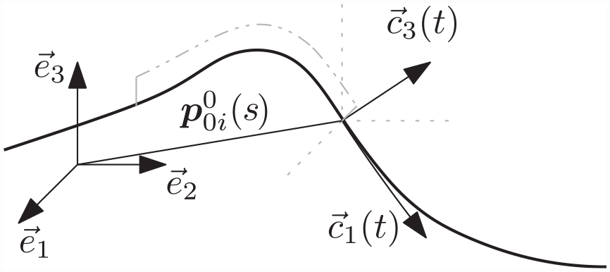
A parametric curve in space.
Notice that
where
A frame local to the origin of
where

where

Finally, the representation of a skew-symmetric matrix is denoted by a hat notation yielding
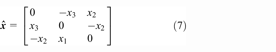
with
2.1. Formulation of equations of motion
In this section, we introduce Kane’s formulation for establishing the equations of motion for a multi-body system. The equations of motion are then expressed in coordinate form.
The force and torque equilibrium of a rigid body

where
To arrive at the equations of motion, the principle of virtual work and virtual displacements are used. The virtual displacement of a particle
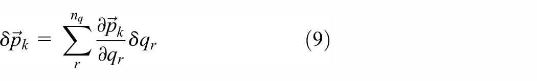
where
where
Multiplying the virtual displacements with Equation (8) yields
where
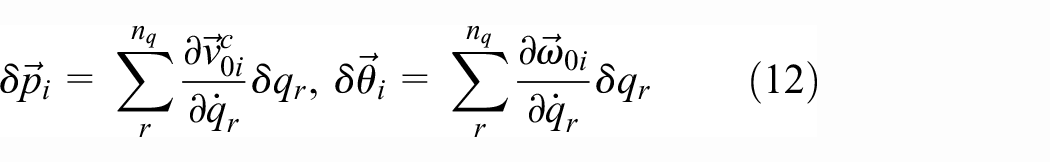
where
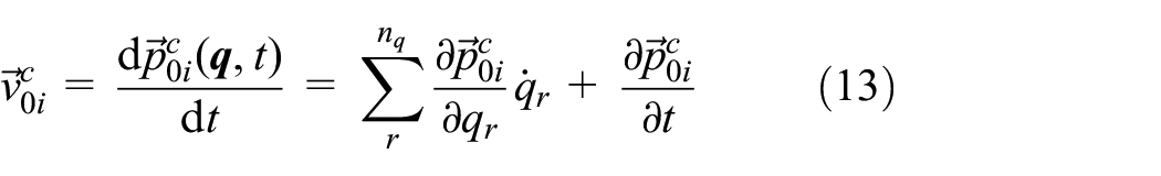
and furthermore, the partial derivative of Equation (13) with respect to
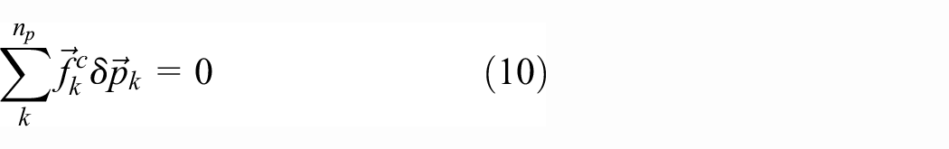
Summing over the number of bodies
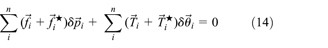
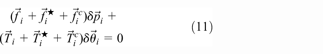
where the principle of virtual work has been used to eliminate the constraint forces and torques. Inserting for Equation (12) for body
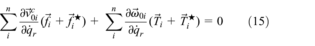
by considering that the variations in
In Kane and Levinson,
19
the linear and angular velocities of
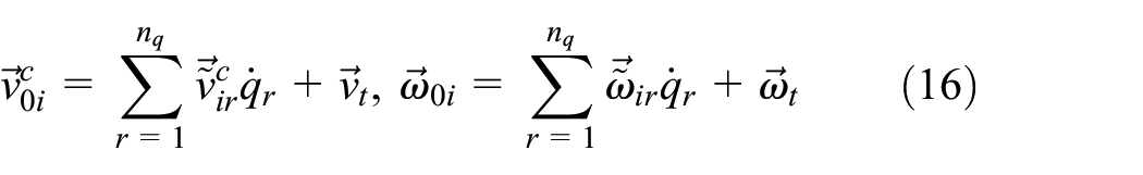
where
The general form of the equations of motion by Kane and Levinson
19
denoted Kane’s equations, can be obtained from Equation (15) describing the dynamic equilibrium for body

where
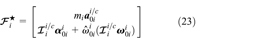
The projection of the inertia forces and torques on
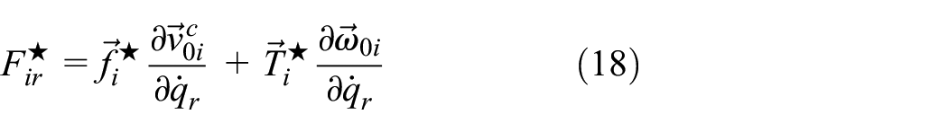


where
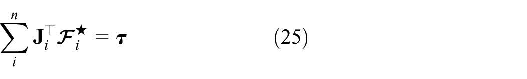
Performing a summation over
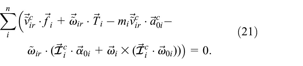
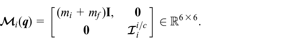
A coordinate form representation of Equation (21) is given next. A projection matrix is formulated for body
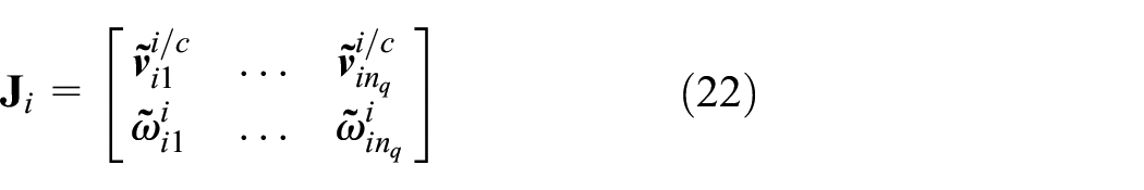
where
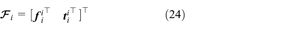
where
Premultiplying Equations (23) and (24) with the transpose of Equation (22) yields
where
For systems exhibiting compliance and damping effects, such as a drill string, Equation (25) can be extended to
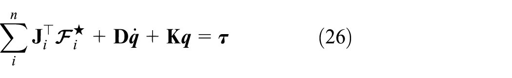
where
3. Wellbore and drilling system representation
The wellbore and drill string kinematics are presented in this section in order to build a simulation model for experimental studies in drilling conditions. The drill string is in this paper assumed to be residing on the center of the wellbore curve
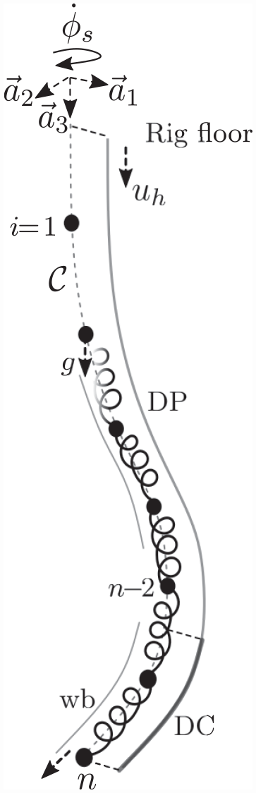
Drill string system confined in a wellbore (wb). The nomenclature is DP—drill pipe, DC—drill collar. At the drill rig floor, a top drive rotates the drill string with to achieve pipe rotational velocity
The representation is based upon the work in Tengesdal et al.
21
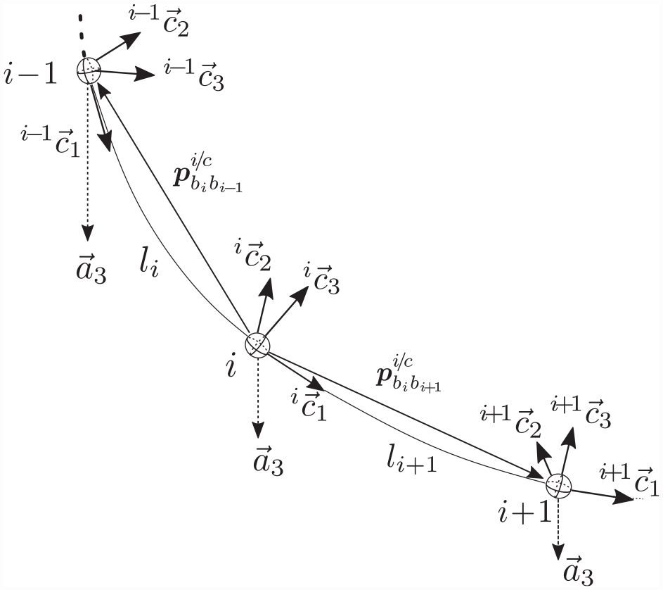
for drill string models in two dimensional space being discretized into lumped masses. The model in this paper is developed for 3D space. Each of the model elements
A set of assumptions is applied to the derivations followed in this paper, and are outlined below:
Assumption (1). We assume that the curve
Assumption (2). The drill string element has uniform density, and a symmetric cross-section.
Assumption (3). The wellbore is circular, defined by the diameter
Assumption (4). The rotation about the normal and bi-normal axes of
Assumption (5). The distributed properties of the drill string assembly can be described by discrete masses with inertia, connected by massless springs, reducing the system into finite dimension.
The curve
Wellbore profile and curvature. The parameters
The drill string model can ultimately be described by the equations of motion similar to what was introduced in section 2 as

where
Hence, the objective is to generalize a model with the above formulation, comprising of four degree-of-freedoms (three translatory and one rotational), coupling of rotational and lateral motion due to eccentricity in the elements, external forces due to contact and input from the rig, and internal forces describing the elasticity of the structure. Moreover, the lumped-element configuration presented in this paper is developed with non-rigidly attached elements as illustrated in Figure 2. Furthermore, the work in this paper is limited to off-bottom analysis.
3.1. Kinematics
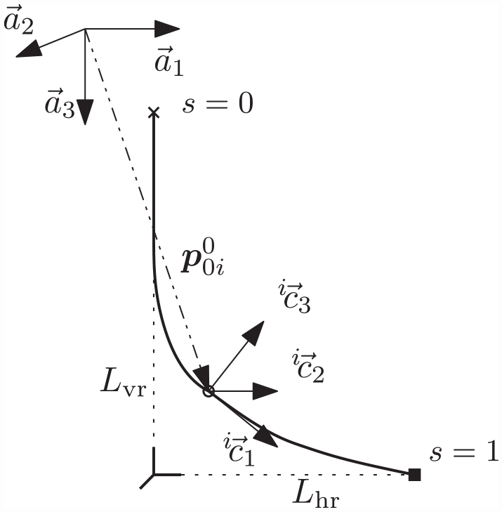
The static wellbore curve

where the bold notation denotes a column vector,
Suppose that a survey point,
From Figure 4, the body frame
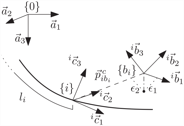
Illustration of the fixed frame for a point along
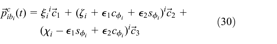
The center of mass can be shifted from the geometrical center
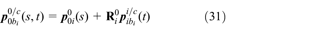
The origin of the element frame
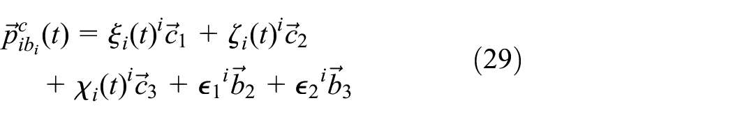
where superscript
where
where

where
3.1.1. Remark
For completely straight wells, we have
Since the curve
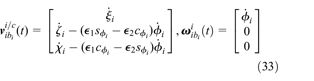
and the linear velocity of the origin of
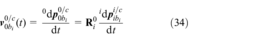
since
The generalized coordinates define the configuration of the system, comprising of

where
A velocity vector can be expressed as
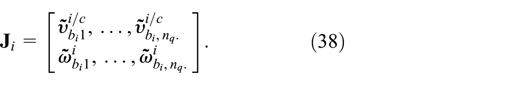
and the partial linear and angular velocity associated with
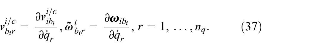
from which we can define the projection Jacobian as
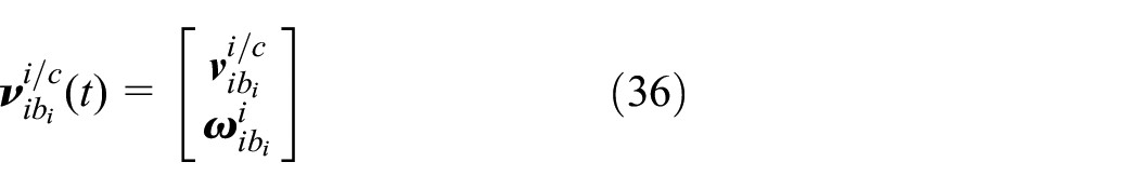
The vector in Equation (36) and its time-derivative are expressed in terms of the generalized velocities using Equation (38) given by Egeland and Sagli 20 as
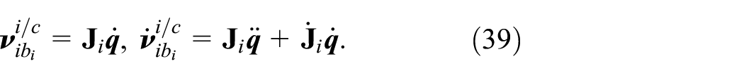
where
4. Drill string dynamics
The distributed motion of the system is discretized into
The configuration is shown for
The mass points located at
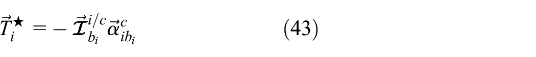
The drill string element inertia forces of the center of mass yield
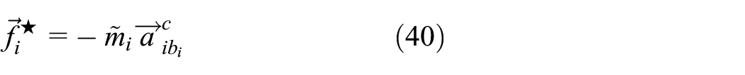
where
where
The inertia torques are given as
where
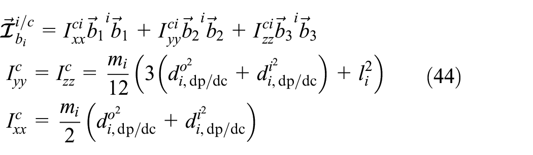
where
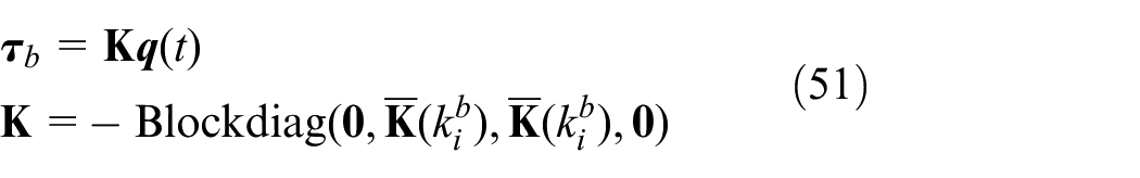
The internal forces and torques contribute to restoring the structure to its original configuration and resist elastic deformation. Assuming that a mass-less spring element connecting
where
The restoring torques about the centroid axis are given as
where
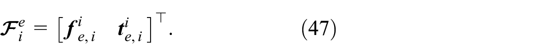
The vector of tension forces and restoring torques imposed on element
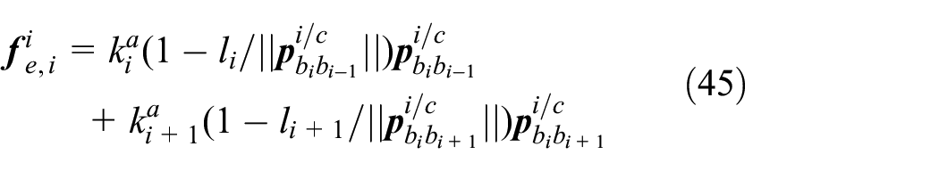
The tension-induced forces comprise the axial stiffness of the drill string, and the coupling to the transverse motion along the assembly. To include the effect of bending moment, a linear approach by superposition on the generalized coordinates is taken. The forces on each element due to bending can be derived from the potential energy, yielding
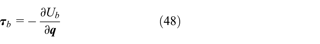
where the term
From Figure 5, the angles formed from a change in lateral perturbation from nominal configuration at
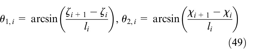
where
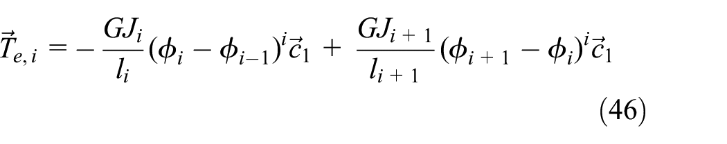
The lumped bending moment can be derived considering the potential energy of a rotational spring, located in each frame
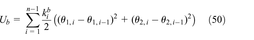
where
where
The gravitational forces are included assuming equal fluid densities inside the drill string and annulus. Hence, the buoyancy factor is expressed according to Aadnøy and Andersen 23 as

where the gravitational forces acting on
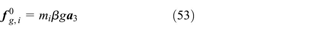
where
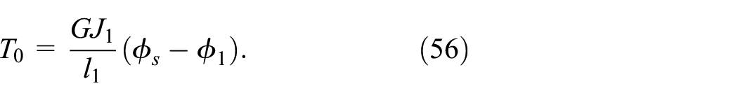
The traveling block adjusts the vertical position of the drill string in the drilling rig. The control input is the block velocity, used to manipulate tripping speed. A change in block position results in a reaction force at
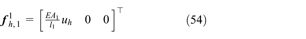
where
The applied torque from the top drive connection shaft yields the torque input to the first element of the drill string. From the shaft rotation angle, given by the drive system, the input torque is given as
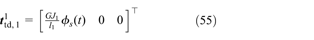
which is applied at
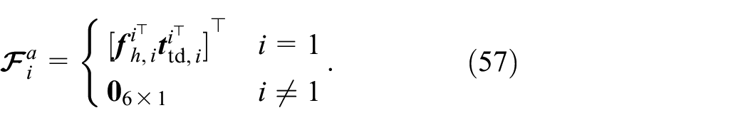
The applied forces from the block and drive are then
Drag forces due to pipe motion in the surrounding fluid are assumed to be proportional to the linear and angular velocities. The effects of damping are included by considering possible turbulent and laminar flow from viscous drag forces. We can express the forces and torques from fluid drag as 24,25
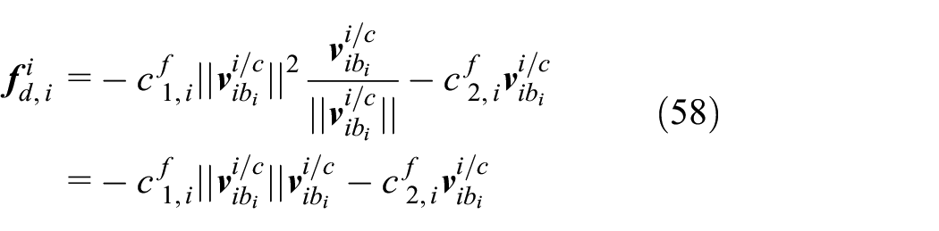
where

and
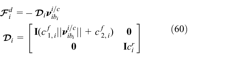
where
4.1. Wellbore contact and friction
In this section, we define the interaction forces due to the transient motion of the drill string in the wellbore. A pipe cross-section is presented in Figure 6 in the normal and bi-normal plane, i.e., the local
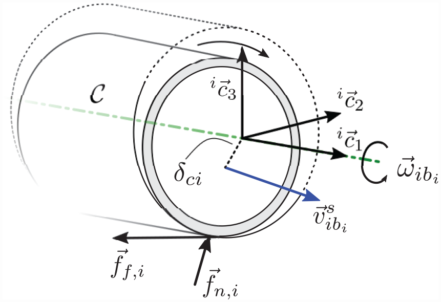
Drill pipe or collar in contact with wellbore wall. Note that all the forces and torques are lumped to the
The impulse response from drill string contact with the wellbore formation can be expressed by a penalty formulation,14,24 being derived next.
The element
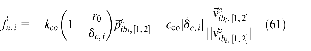
where
A friction force perpendicular to the contact normal force and in the opposite direction of the segment velocity is generated at the point of contact. The slip velocity between the two surfaces (pipe and wellbore) in contact (as sketched in Figure 6) can be expressed as 26
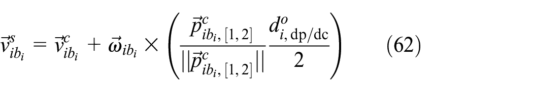
where
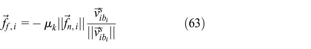
where
The frictional torque due to contact is given by the magnitude of the friction force, expressed as
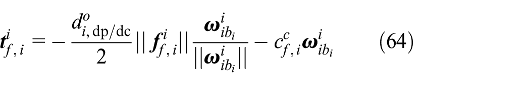
where the rightmost term denotes the viscous torque proportional to element angular velocity.
The contact forces and torques are summarized as
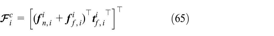
4.2. Equations of motion
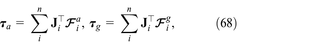
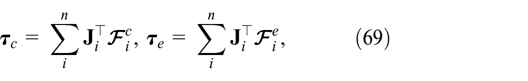
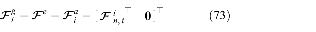
The equations of motion are formed using Equation (26) with Equations (40) and (43), and together with the defined generalized active and restoring forces and torques, given as
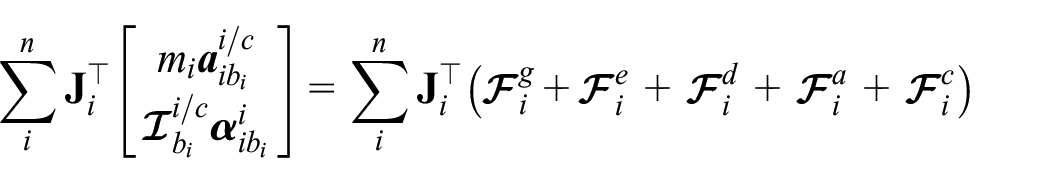
which can be rewritten using Equations (39) and (60) as
where
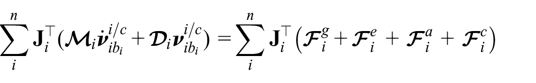
Adding in the forces resulting from linear bending in Equation (51), and using the generalized velocities in Equation (39), we get
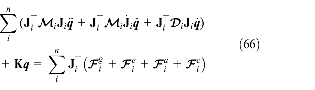
and hence, the equations of motion of the drill string system can be written as second-order ordinary differential equations including the linear bending stiffness, yielding

where
where
5. Steady-state configuration
The LM configuration imposed by the elastic deformation described by Equation (67) is in this section compared to a similar FEM model in Abaqus, an acknowledged commercial software for finite element analysis (FEA). For linear analysis, the B21 element is used, which is a 2-node linear beam in a plane. For nonlinear analysis, the B22 element is used, which is a 3-node quadratic beam in a plane. The analysis is performed to validate the elastic force contributions in the LM, which represents bending, given by the lateral displacement of each element.
For a deviated wellbore configuration the drill string model in Equation (67) is deformed by gravity in both the lateral and longitudinal directions, where both the axial stiffness and bending stiffness of the pipe affect the configuration. To verify the steady-state solution of the linear bending forces, the two effects are isolated in separate tests: a vertical and a horizontal configuration.
The drill string is stretched due to the structural weight, and under the influence of gravity and buoyancy with mud present in the annulus. We assume that the wellbore is arbitrarily large, i.e.,

where
5.1. Free-hanging vertical solution
The vertical hanging static case is compared with the FEA results, and we assume that the drill string only subject to its dry-weight, hence
Case 1 parameters.
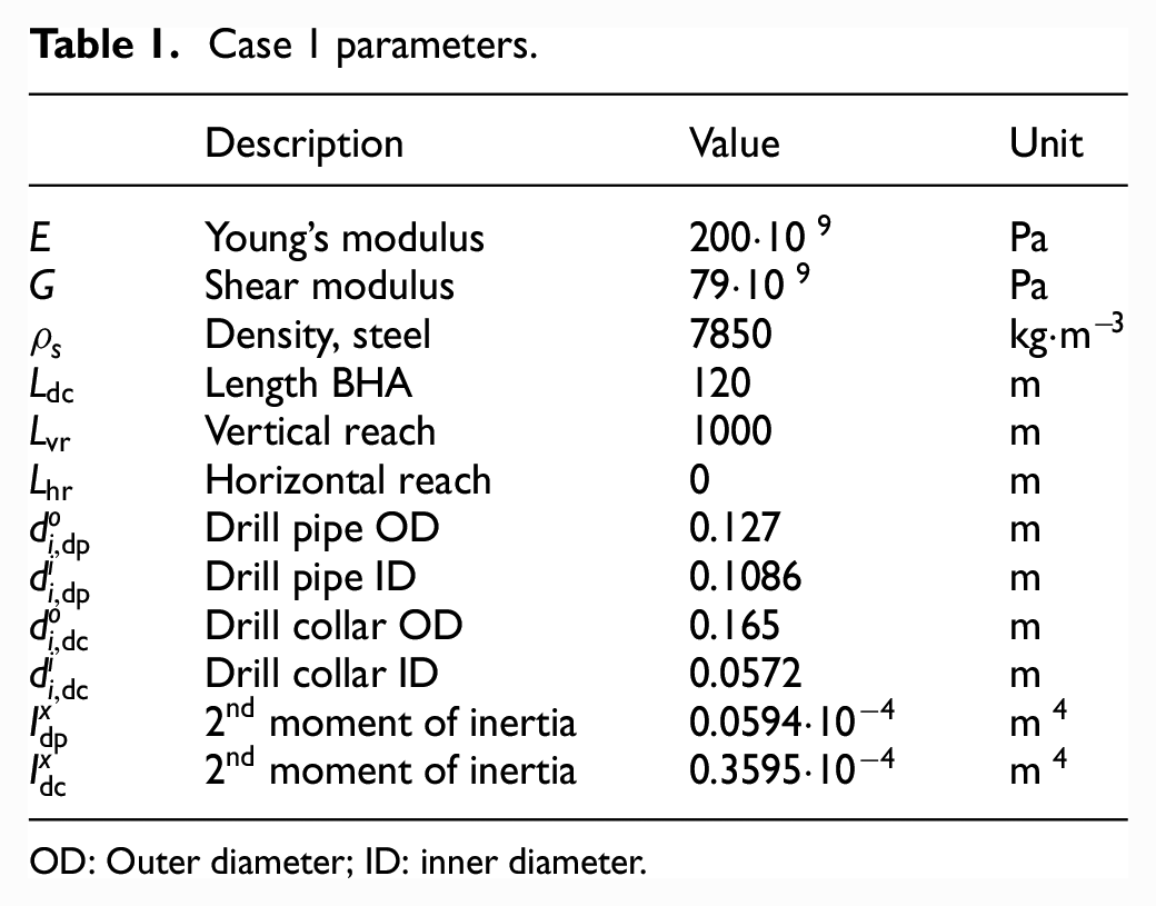
OD: Outer diameter; ID: inner diameter.
The displacements at six locations from discretization of the vertical drill string configuration into 10, 20, and 100 lumped elements are compared with the converged FEA solution. The displacements are shown in Figure 7.
Static configuration for Case 1, with converged FEA solutions for comparison.
The general observation in Figure 7 is that by increasing
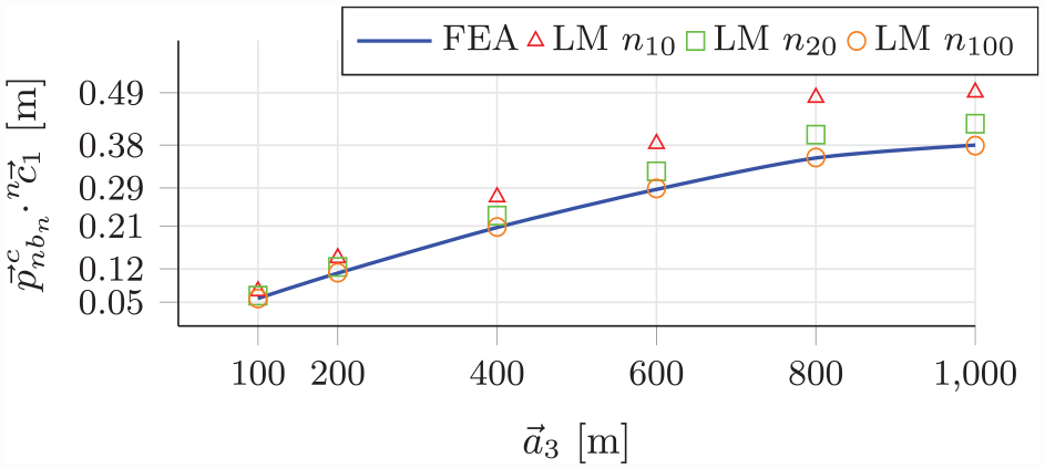
5.2. Convergence to a horizontal solution
A simply supported beam in horizontal orientation with a pinned-slider boundary condition is used to verify the forces due to bending and tension. The model representation is depicted in Figure 8.
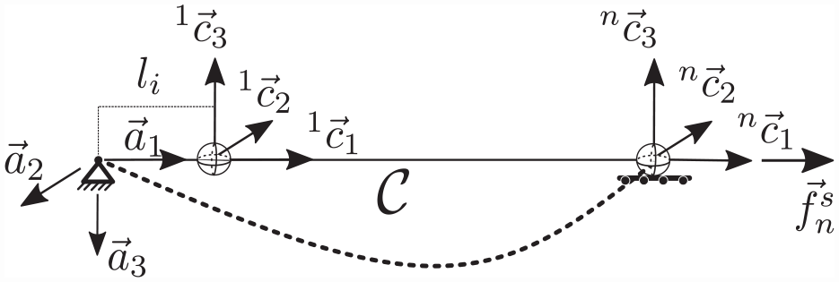
Static configuration for Case 2. Dotted line represents a sketch of the deformed configuration.
A static force,
The LM is moment free at
The supporting forces acting on element

where
The Case 2 parameters different from Case 1 are given in Table 2. Three values of the acceleration of gravity constant
Case 2 parameters for
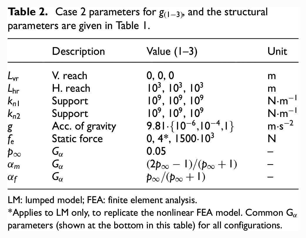
LM: lumped model; FEA: finite element analysis.
Applies to LM only, to replicate the nonlinear FEA model. Common
The Generalized-
For pipe weights with
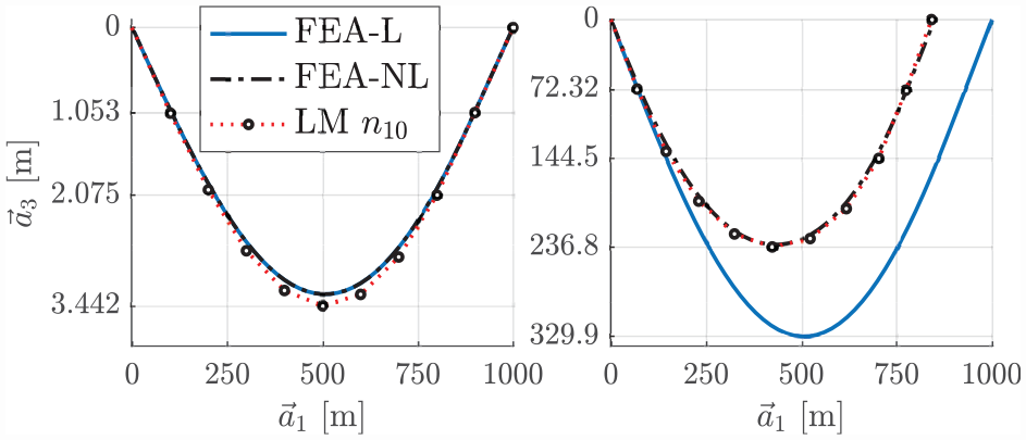
Drill string curvature due to internal weight with
In the leftmost plot, for the loading conditions with the lowest acceleration of gravity and zero horizontal force, the linear and nonlinear converged FEA together with the LM shows similar results. The FEA solution is discretized into 20 m long elements, leading to a total of 50 elements. For this configuration the bending stiffness governs the shape of the drill string.
When the gravity is increased, as seen in the rightmost plot in Figure 9, the linear analysis will start to deviate from the nonlinear analysis. The nonlinear analysis for both FEA and LM also shows the contraction of the pipe due to coupling to the axial tension, with a negative horizontal displacement.
When
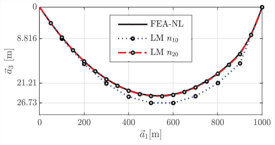
Drill string curvature due to internal weight with
A close match with the FEA is shown both for the pure bending case and for the more involved case of large deformations. Since many of the significant effects such as complex geometrical stiffening effects are neglected in the LM, deviations are evident.
The elasticity of the LM increases the time for its structural configuration to reach steady state. In addition, the displacement is only an effect of the imposed external and restoring forces. Hence, our model converges to the free-hanging physical configuration of the drill string when the number of elements increase. Similar conclusions were drawn for a simplified discrete rod analysis in Dreyer and Vuuren, 30 however, without axial contraction between the model elements.
6. Simulation and results
In this section, a simulation study is performed, and the qualitative properties of the model are presented. The numerical solution forward in time
Model parameters with
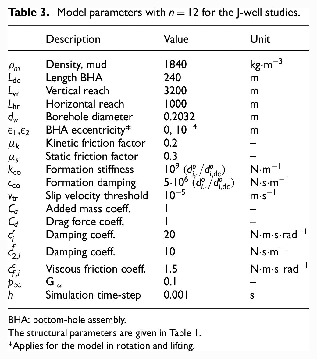
BHA: bottom-hole assembly.
The structural parameters are given in Table 1.
Applies for the model in rotation and lifting.
The friction forces are modeled by Coloumb friction in Equation (63). These forces balance the inertia and external forces on

where

where
6.1. Block and torque control
We assume that we can manipulate the traveling block velocity in terms of controlling drill string position in the wellbore. The block is subject to heave and velocity control from the driller, and its position is defined by the block position input
A variable speed drive (VSD) controls the torque supplied to the drill string. For the purposes of including a dynamic top drive model, the motor is given as

where
Using a proportional-integral (PI) controller, the input torque supplied by the VSD is computed from the desired top-of-string angular velocity, yielding
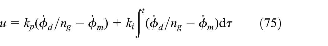
where
Top drive parameters.
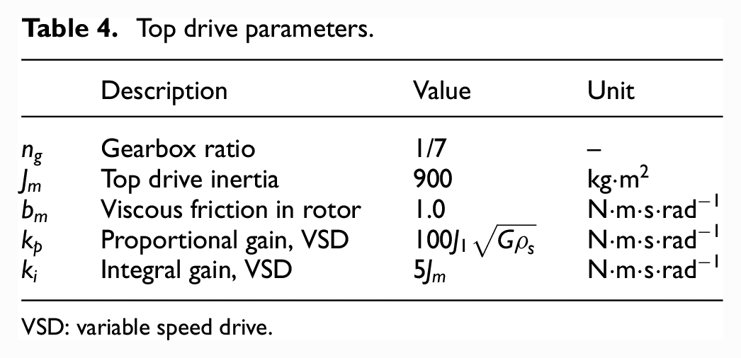
VSD: variable speed drive.
6.2. Surge and swab pressures
The pressure profile in the wellbore is an important parameter for monitoring and maintaining well-stability, by safeguarding the drill string velocity. In this section, we include a static model for computing the wellbore annular pressures. Hence, no coupling is included such as the effect of damping of drill string vibrations due to mud flow (see, e.g., Wilson and Noynaert 4 ).
During drill string movement, the pressure profile in the wellbore is subject to surge (running the drill string down in the well) and swab (retrieving the drill string) pressures. To avoid large surge and swab pressures causing instabilities in the well, the tripping velocity of the block is manipulated.
A symmetrical cross-section of the element was assumed, and we neglect the mud flow variations due to tool joints. The average mud flow velocity can be calculated assuming closed pipe ends, when all the fluid is displaced upward in the annular section.
33
The mud velocity is given by the pipe velocity of the
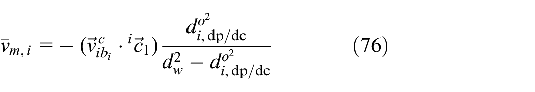
where
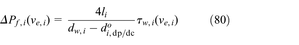
The pressure loss over the drill string segment is a function of mud flow velocity and its flow regime. The Darcy–Weisbach equation can be used as an approximation to obtain the pressure loss due to pipe movement. 34 It is defined as
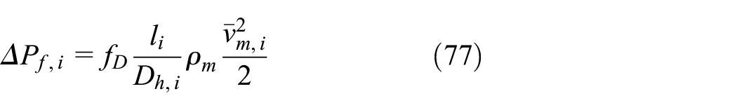
where
In annular flow, where the inner section moves and the outer section is stationary, it can be useful to define the effective velocity,17,33 given as

where
The laminar and turbulent flow regimes are used to characterize the Darcy friction factor
where
An estimate of the bottom hole pressure (BHP) is then obtained as

where
6.3. Heave-induced pressure oscillations
In this section, the drill string is fixed in the drill floor slips during pipe connection. Hence, the drill string is subject to heave motion from the rig.
A simple wave characteristic is assumed, where the heave amplitude and wave period are the only parameters considered. 35 The rig floor position due to heave is given as

where
At time
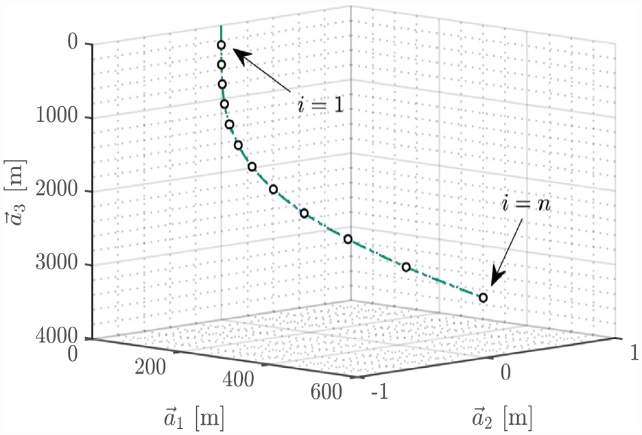
Wellbore configuration with model element position indicated by circles.
The drill string is being suspended in the rig-floor slips at
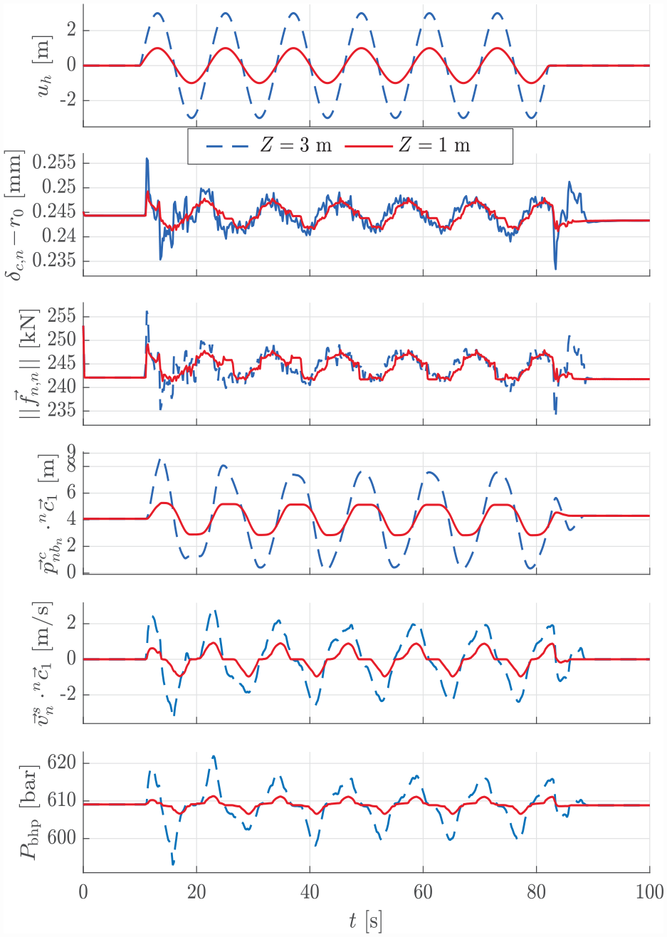
The effect of heave due to fixation in rig floor slips. Solid line represent wave height of 2 m, and dashed line for wave height of 6 m.
From plots two and three (counting top-down) in Figure 12, the clearance variable
As observed from Figure 12, in plot four and five the bit sticks for a moment during the wave top. This correlates with plot five showing the slip velocity, where axial stiction is obviously occurring for lower heave amplitudes.
6.4. Rotation while lifting
To evaluate the consistency of the model toward coupled rotation and translatory motion, we utilize the same wellbore and drill string configuration as in Section 6.3. A pipe-stand trip sequence is performed with and without rotation, to illustrate some transient characteristics related to axial friction while rotating.
Tripping out one stand and running it back in is seen in the first 90 s of Figure 13(a) and (b) for
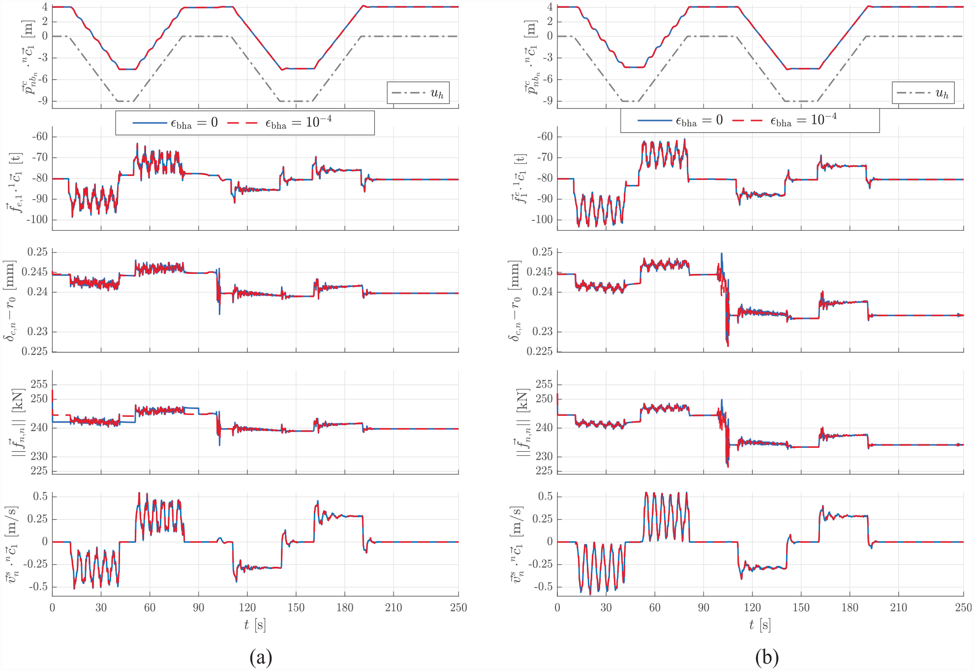
Rotating while running out and back in one stand. For solid lines the BHA elements has
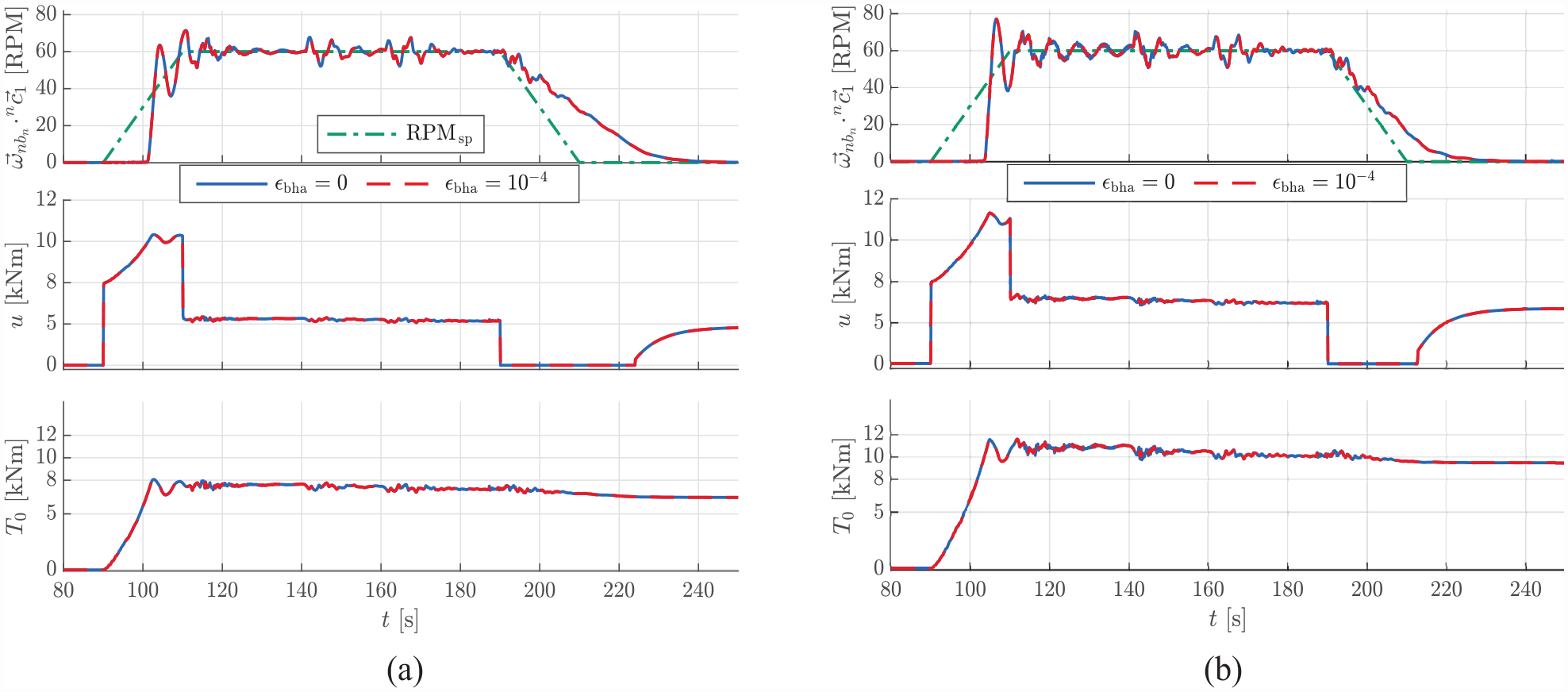
Down-hole bit angular velocity and motor and top-of-string torque while running out and in the drill string one stand. For solid lines the BHA elements has
The tripping velocity is
The intention of rotating while pulling is to reduce axial drag and friction between the drill string and the wellbore. 36 We observe from the second plot in Figure 13(a) and (b), that the tension difference in the uppermost segment of the drill string reduces by around 5 tons when rotating and tripping. The lowermost plot shows the slip velocity at the bit, seen to be dampened out due to increase in the angular velocity of the bit.
Increasing the friction coefficients in the model tends to lead to a slight increase in the uneven bit axial motion (topmost plot of Figure 13(b)) during tripping without rotation, and a general amplification of the upper segment tension and slip velocity. The bit angular velocity also experiences an increased oscillatory pattern, as seen in the topmost plot in Figure 14(b).
7. Discussion
In this work, no model for axial bit–rock interaction and coupled torque-on-bit has been included. Improvements in future work involve extending the model applicability to downhole conditions. Furthermore, comparison toward similar models and field data are steps to further establish the validity of the model. The authors do not presently have access to field data for comparison. As any well described by a parametric curve can be implemented, a realistic well from work such as Aadnøy and Andersen 23 could facilitate further model validation. The rest of this section includes a discussion on model effects and a study of two numerical integration methods.
7.1. Geometrical stiffening effects
The drill string is confined in the borehole such that limited lateral movement is allowed, and the curvature at
7.2. Selection of numerical solver
The numerical stability dictates the performance during the simulation and accuracy of the results obtained. For second-order models used to represent drill string dynamics, the method by Newmark
28
(see, e.g., Wilson and Noynaert,
4
Butlin and Langley
37
), Runge–Kutta, and the forward Euler methods12,38 are among some of the more common integration schemes found in the literature. Nonlinear models comprising contact dynamics and stick-slip behavior may require a relatively short time step
The stability region for a Runge–Kutta method of order 4 in terms of an undamped oscillator can be drawn from Hairer and Wanner, 39 Figure 2.1, yielding

where
In our model, the contact forces generated from drill string element impact with the formation is given by the penalty model in Equation (61). In free hanging form, boundary conditions alter the eigenfrequencies of the drill string in each of the degrees-of-freedom. However, when contact occurs, the formation stiffness is typically larger than the structural stiffness. For the Generalized-
The time step for a simulation sequence has to be set according to the relevant frequencies in the system. Typically, when including a penalty-based model for the wall impact, the formation stiffness dictates the magnitude of the system eigenfrequencies. The eigenfrequency of the drill string when in contact with the wellbore can be given as
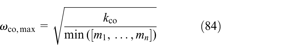
where
For an RK4 method the maximum time-step size for a stable RK4 solver can be predicted for the drill string. For the simulated cases with
7.2.1. Brief comparison of solvers
This section gives a comparison of applying an RK4 and a
where
The block position is given by a periodic function
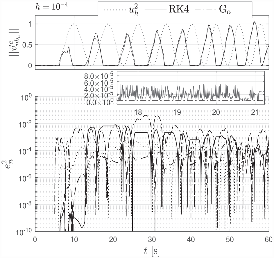
Comparing
The square of the input to the block, along with the norm of the bit velocity for
Comparing RTFs for simulation studies in this paper.
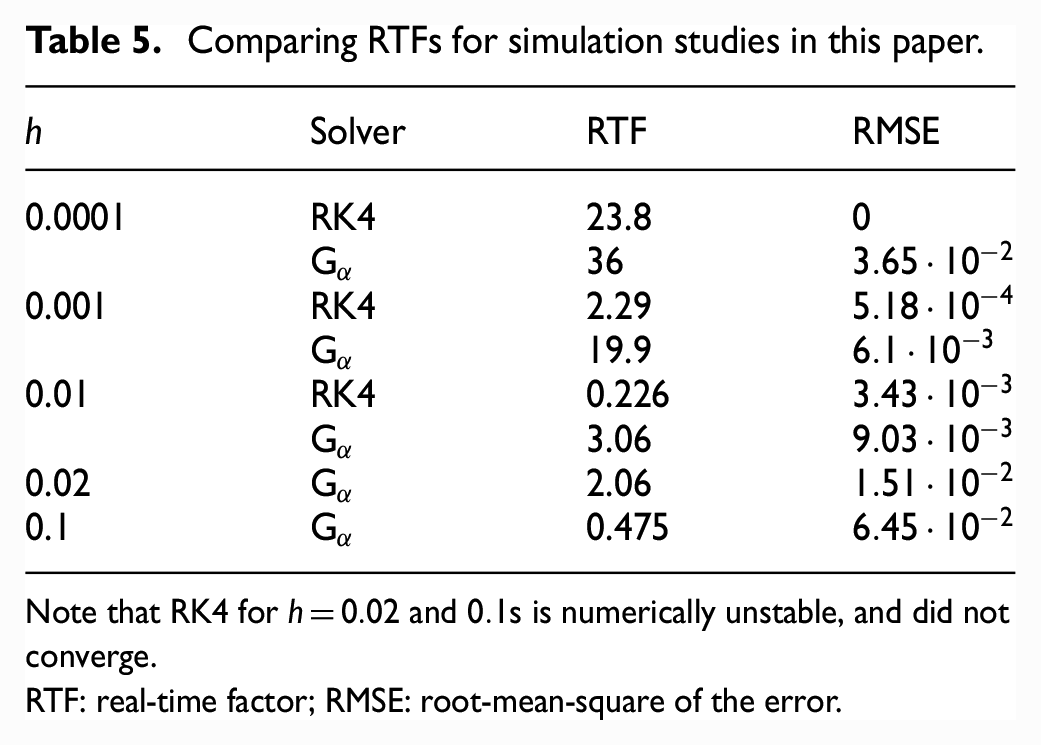
Note that RK4 for
RTF: real-time factor; RMSE: root-mean-square of the error.
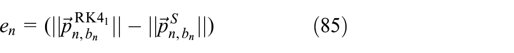
The RMSE is computed from
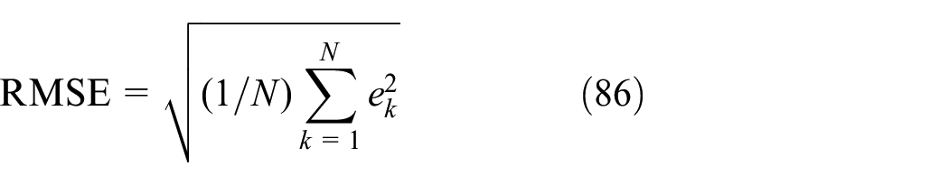
where
The
8. Conclusion
From the work presented in this paper, we have proposed an LM for analyzing transient drill string motion in arbitrary wellbore configurations. The wellbore is represented as a parametric curve in space, and the equations of motion are derived using Kane’s method.
A static configuration test toward FEA acting as a benchmark was performed. The LM, subject to axial tension and linear bending stiffness, conforms with the FEA for completely straight configurations. Evidently, increasing the number of elements in the discrete model yields better agreement. The model axial friction forces and contact forces were analyzed in two simulation studies for a deviated J-well drill string. The first presented the behavior during pipe connection, and the second showed the effect of rotating while tripping the drill string. Well-known characteristics such as reduced axial tension due to rotation were confirmed in simulation. A PI torque controller was implemented, along with manipulation of the block velocity.
The model computational efficiency in terms of error propagation and simulation time is compared with a Generalized-
Footnotes
Appendix 1
Funding
The research presented in this paper has received funding from the Norwegian Research Council, SFI Offshore Mechatronics, Project No. 237896.