Sage Journals: Discover world-class research

Abstract

Precise navigation for fully autonomous driving—especially in dense urban areas—requires periodic precise position estimates. Global Navigation Satellite System (GNSS) technology has the potential to provide absolute positioning accuracy at a centimeter level. However, buildings in urban environments cause signal distortions and signal reflections—the so-called multipath—which are the most challenging parts in the GNSS error budget. Hence, we developed a scalable real-time multipath simulator for mitigating potential multipath receptions. The simulator uses three-dimensional (3D) building information, satellite, and user positions. The key drivers of latency are the calculation of reflection, diffraction, and line-of-sight, as well as the response time of the 3D building model database. The memory manager of the graphic processing units (GPUs) in combination with a dedicated load balancer enables fast and efficient multipath analysis. Selected case studies demonstrate the simulator’s potential to significantly improve the position accuracy of the processing engine. The use of the multipath simulator reduces the error in 61% of the error measurements in a stress test scenario to less than half of the non-multipath processing. The scalability of the simulator is demonstrated by combining the multipath simulator with a traffic simulator. Furthermore, we present a novel methodology for the detection of walls using GNSS signals to better account for incomplete or erroneous 3D building information in GNSS signal processing.

Keywords

Real-time simulation multipath ray tracing urban GNSS positioning city GML GPGPU

1. Introduction

The real-time navigation in unknown dynamic environments has become an increasingly important topic in modeling and simulation. Path planning and decision-making can guarantee that participants reach their destinations without colliding with obstacles and other participants in an optimal way.¹ Recent works in this field of research addressed the collision avoidance and path tracking problems. An affective computing-inspired driving controller to avoid rear-end collisions is presented in Butt et al.² A method for lane and obstacle detection using a camera module on a mobile robot is demonstrated in Singh et al.³ In Sun et al.,⁴ a Global Navigation Satellite System (GNSS)/compass fusion with the Adaptive Neuro Fuzzy Inference System (ANFIS)–based algorithm for real-time car-following status identification is developed. The GNSS/compass-ANFIS-fusion approach relies on localization coordinates with centimeter accuracy, which is not guaranteed in urban environments.

Many urban navigation applications (e.g., autonomous driving or driver assistance systems) require localization with centimeter accuracy.⁵ A localization system identifies the location, e.g., of a vehicle (in GNSS literature often referred to as “rover”), in a global coordinate system.⁶ The localization methods can be categorized into: active sensors (including transmitters that send out a signal which is echoed by the target and the sensor capturing the echoed signal) and passive sensors (collecting data, including light, radiation, heat, or signals in the surrounding environment).⁷ GNSS technology, a passive sensor–based localization method, has emerged as a well-established technology for several outdoor applications with high reliability and accuracy demands.⁸

In urban environments the occurrence of satellite signal reflection and diffraction, e.g., due to surrounding buildings, also called multipath, remains challenging.⁹ One approach to face this issue is to separate direct line-of-sight (LOS) signals from faulty satellite signals (typically caused by multipath or non-line-of-sight (NLOS)) using a consistency check.¹⁰ A second approach is to detect static and dynamic objects, which cause obstruction of direct satellite vehicles (SVs) visibility, using the three-dimensional (3D) light detection and ranging (LiDAR) method and exclude NLOS signals in the positioning engine (PE).¹¹ A third approach could be the use of 3D building information to improve the positioning quality. Recent works, where 3D building data were used, include integration of other sensor data (e.g., inertial sensors),¹² removal of NLOS satellites,¹³ shadow matching (identification of the measured LOS-NLOS-pattern in an LOS-NLOS-map created with 3D building data),¹⁴ or correction of the measured pseudo-ranges.¹⁵ In addition, simulation-based analyses of multipath propagation in urban environments are under development using ray-tracing techniques.^16,17

Multipath simulators for real-time applications are designed to either be efficient or provide a high degree of realism. Efficient simulators are able to model the multipath situation with very low energy and hardware requirements, but have limitations such as incomplete building representations and high computation latencies. An example that has a typical processing time between 1 and 2 s is reported by Wang et al.¹⁸ Another real-time simulator focusing on efficiency was developed in Wang et al.¹⁹ The simulator calculates the boundaries of buildings from the rover’s perspective for some candidate positions of the rover in advance and assigns the rover position to the closest candidate position. Recent work by Google in the area of efficient multipath simulators in real-time applications has achieved promising results using Android phones. A 50%–90% reduction in the frequency of wrong-side-of-street occurrences by GNSS in phones has been obtained.²⁰ Instead of solving the computational load (which is by far too much for an Android phone) straight forward, the Google approach uses machine learning to compute GNSS locations. An example for a multipath simulator that offers a high level of realism is Spirent Sim3D. There, vegetation, traffic, crowd, and other arbitrary objects, which might impact the multipath situation, are considered. The limitations of the Sim3D simulator are the restriction to specific hardware, the spatial restriction of model data $(5 k m^{2})$ , the update rate of at least 100 ms, the limited number of multipath rays per LOS, and the maximum number of one receiver per installation.

In practice, 3D building model information must be used with caution due to its accuracy and incompleteness. In Voelsen et al.²¹ and Zou and Sester,²² a mobile mapping LiDAR system is used to map changes of the environment and refine the building model information using generated point clouds, respectively.

We present the continued research of our recent publication on a low latency multipath simulator.²³ The implementation of the multipath simulator is shown, and the results of a performance analysis using 3D building model data of the city of Hannover are presented. The localization performance is evaluated by comparing topocentric deviations to a reference position. We demonstrate that the multipath simulator significantly improves the positioning accuracy. Another performance criterion is the response time or latency. Our multipath simulator can handle several requests from moving receivers in parallel while the receivers can be distributed in the entire city without significantly increasing the response time. In addition, a wall detection algorithm is developed, which is able to generate building model polygons based on a known user location and GNSS observation, e.g., to perform ray-tracing techniques when the building model is incomplete.

The structure of this paper is as follows. An overview on how the multipath simulator and the wall detector are embedded in the localization procedure is presented in section 2. Implementation details of the multipath simulator computation core are described in section 3.1. The multipath simulator operates with vast amounts of data. The organization of memory is shown in section 3.2. Several PEs might connect concurrently to the simulator. The distribution of the workload to all available graphic processing unit (GPU) hardware is described in section 3.3. The new method of wall detection is presented in section 3.4. The validation of the simulator in terms of localization improvement is presented in section 4. Factors affecting the response time behavior of the multipath simulator are analyzed in section 5. The results of the novel method for wall detection in urban environments based on GNSS signal analysis applied to a courtyard scenario are presented in section 6. The conclusion is drawn in section 7.

2. Multipath simulator and wall detector

The multipath simulator is a server-based software. The client software, which is able to connect to the multipath simulator, is installed on objects, which move through an urban area and carry GNSS antenna and receiver hardware. The purpose of the multipath simulator is to analyze and classify the multipath situation of the GNSS antenna in a 3D building model environment. Based on the ray-tracing results and the GNSS measurements, the client software (PE) computes the position of the user antenna.

The interference of multipath is caused by signals that arrive at the user antenna via indirect paths. As depicted in Figure 1, indirect signal paths from the satellite to the receiving antennas are caused by reflections from one or multiple objects (buildings, ground, etc.), signal diffraction, or a combination of both effects.

Figure 1.

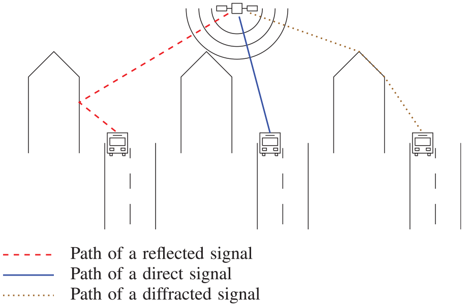
Signal reflection, direct signal, and signal diffraction.

Figure 2 shows how the simulator is embedded in the positioning data flow. Initially, a rover is moving through an urban environment capturing and providing GNSS observation data to the PE. The PE sends a request to the multipath simulator, which consists of a rover ID, a position estimation, and a time stamp. Generally, the position estimation can be computed using the previous positions in combination with a motion model. The multipath simulator requests corresponding ephemeris data, i.e., GNSS satellite orbit data, from a satellite ephemeris database and 3D building model data, i.e., sets of the so-called triangle meshes, from a building model database. Once, the multipath analysis is complete, the simulator responds to the PE with its ray-tracing results. In the simplest configuration, a list of SVs, which should be ignored in the current processing epoch, is send. In an advanced setting, a list of residuals per SV is send to the PE. The residuals are an approximation of the extra path delay of the received signal, compared to the direct LOS.

Figure 2.

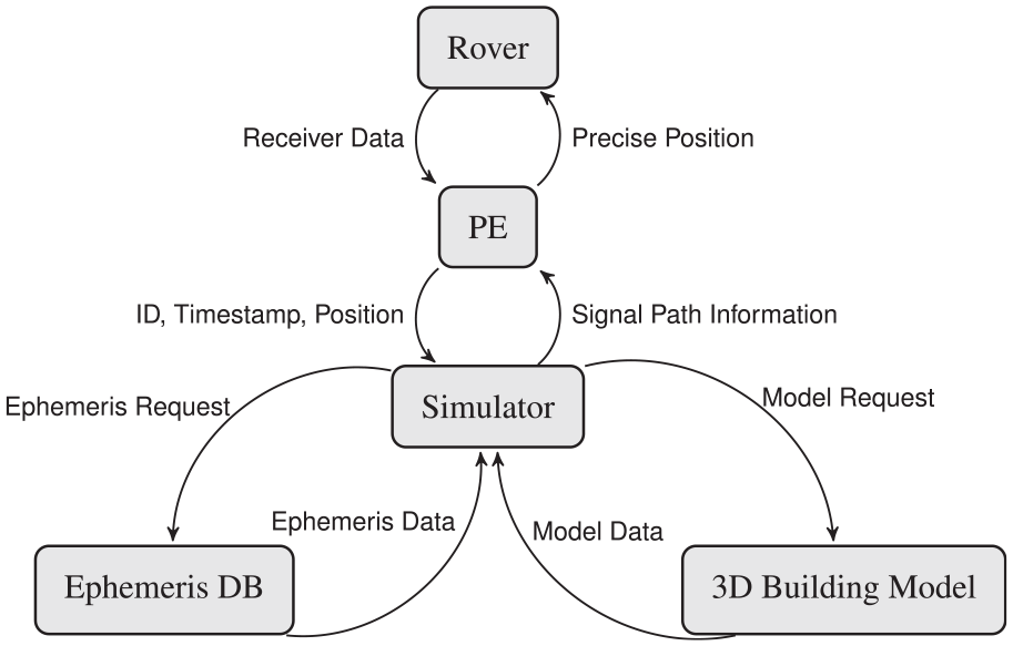
Data flow of positioning with multipath simulation.

Technically, the rover can be any object equipped with a GNSS antenna and receiver (vehicle, smartphone device, unmanned aerial vehicle, etc.). However, the components of the data flow are designed with suitable latencies, according to vehicles that follow the traffic rules in urban areas. The response time experiments in section 5 handle the use case of estimating the location of several vehicles moving on a road network. The queries from the PEs are processed in parallel. The PE of each rover generates a request once in a second and blocks its processing until the response from the multipath simulator arrives. Thus, the time period between the commit time of the simulation request and the receiving time of the response is limited. Typically, the mobile communication user-plane latency (i.e., round trip time according to the specification in 3GPP TR 38.913) can be assumed to be less than 700 ms (600–700 ms for application of GPRS, much lower for more modern mobile communication standards).²⁴ Assuming the processing delay in the users PE to be less than 200 ms, the processing delay of proposed multipath simulator should not exceed 100 ms in order to assure user positioning update rates of 1 Hz including involvement of real-time multipath simulation. Thus, we set the multipath simulator timeout to 100 ms. In case of a timeout, the PE proceeds without ignoring any SV. Therefore, the practical relevance of the simulator for real-time applications is determined by the ability to improve the positioning accuracy (localization performance) while its latency is kept down (response time performance).

The multipath simulator processes a triangle mesh, an estimated rover position, and the SV coordinates to perform ray tracing and provide signal path information. Wall detection using GNSS data is a novel method to create a triangle mesh (i.e., building model) based on the PE results. The created triangle mesh can either be used as an alternative to the external building model (e.g., from a scanning flight campaign) or as a local refinement. This methodology itself does not access the external building model.

There are two fundamental reasons for the need of wall detection: first, the original 3D building model is incomplete, i.e., not all relevant buildings are modeled. Second, the 3D model includes irrelevant parts of buildings such as roofs, ground planes, and interior walls. The wall detector is not running in real-time since it is a method to post-process the PE results from multiple rovers for improving the 3D building model in a localized area. Figure 3 illustrates the required inputs and provided outputs of the multipath simulator and wall detector. The required inputs of the wall detector are SV ephemeris data and the computed results of the PE such as residuals and rover positions. The corresponding output is a triangle mesh that can be used to refine or correct the 3D building model.

Figure 3.

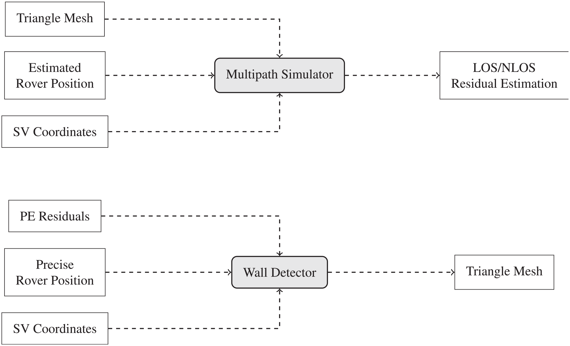
Inputs and outputs of the multipath simulator and the wall detector.

3. Implementation details

The following section gives an insight into the implementation of the multipath simulator and the wall detector.

3.1. General GPU accelerated computation approach

The computational part of the multipath simulator requires (1) a static triangle mesh representing the 3D building model, (2) an approximate rover position at a certain timestamp, and (3) corresponding coordinates of the SVs used in the study, such as Global Positioning System (GPS), Global Navigation Satellite System (GLONASS), Galileo, and BeiDou satellites. Possible blockages of the LOS between user antenna and SV are identified by performing cross-checks for each involved SV. Depending on the configuration, the simulator proceeds with both reflection and/or diffraction analysis.

Figure 4 outlines the processing organization of the multipath simulator. The architecture is designed for multithreaded Single Instruction Multiple Data (SIMD) processors (i.e., GPU programming) and is implemented in OpenCL (Open Computing Language).

Figure 4.

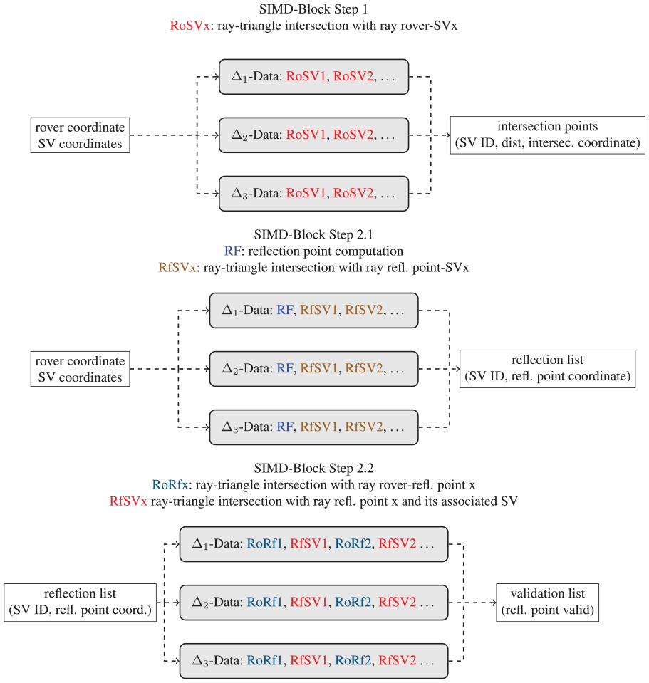
Architecture of the multipath simulator computation core for multithreaded SIMD processors.

In the first step, each invocation of the OpenCL kernel code executes a ray-triangle intersection algorithm²⁵ for each SV. Thus, for every single loaded triangle, a computation instance is started, which processes the ray-triangle intersection algorithm for each SV. The inputs of the ray-triangle intersection kernel are a status_in (number of SVs), the coordinates of the triangle edges (including the triangle normal), and coordinates of the rover and the SVs. The outputs are a status_out (number of detected intersections) and an intersection list consisting of the SV ID, intersection point, and its distance to the rover. If an intersection is detected, an atomic incrementation of the status_out is performed, and the computed intersection information is copied to the intersection list. The detection of an intersection indicates a blockage of direct signal between satellite and user antenna, i.e., the LOS path is not present.

Step two is the reflection analysis, which is divided into two sub-steps: computation of reflection rays and removal of ray-triangle intersecting rays. Each sub-step is implemented as separate OpenCL kernel code and is executed for each of the triangles with a barrier synchronization between the sub-steps. The first sub-step is depicted in Figure 5. For each triangle, an image of the rover is computed, and for each SV, the ray between the image and the SV is computed and the ray-triangle intersection algorithm is applied subsequently. In case of an intersection, the intersection coordinates and the SV ID are added to a reflection list. In the second sub-step, all reflected signal paths, which intersect other triangles, are marked as invalid. Thus, the ray-triangle intersection algorithm is applied for all entries in the reflection list. In practice, reflection paths with multiple reflection triangles are possible. We expect that the signal strength in those cases is sufficiently weak so that the PE is not significantly affected. Hence, in order to save computation resources, the multipath simulator is only identifying paths with one single reflection triangle.

Figure 5.

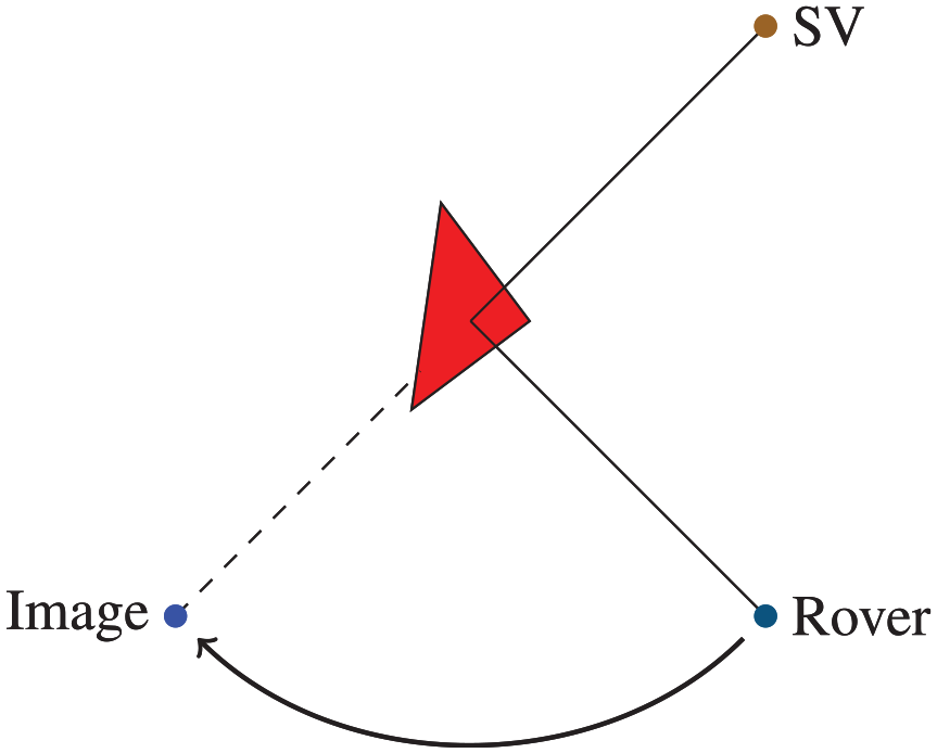
Computation of reflection rays.

The final step of the multipath analysis is the diffraction analysis. This analysis is also divided into two sub-steps, which are executed separately for each SV. In the first sub-step, diffraction path candidates are computed where our algorithm has to deal with different challenges: (1) the versatility of the modeled buildings (non-convex objects with partly unclear meshes) and (2) if two planes of the real building share an edge, they do not necessarily have a common edge or vertex in the building model. Our approach of finding diffraction path candidates is therefore based on the fact that the diffraction path can be modeled with a linear spline function from the SV to the receivers’ antenna position with knots on triangle edges of the building model data. For an example, notice the diffraction path in Figure 1, which has two diffraction points on the buildings: one at the ridge and one at the eaves. Similar to the reflection case, the multipath simulator only computes path candidates with one single diffraction point. So, the multipath simulator is not able to find the diffraction path with two diffraction points shown in Figure 1. In the worst case, a path could even be calculated which is not a valid diffraction path at all. Nevertheless, the experiment results in section 4 show that the limitation to diffraction paths with only one diffraction point is sufficient. A configurable parameter is set for the number of candidates per triangle edge. For each of the loaded triangles, an OpenCL worker thread generates the diffraction candidates and computes its overall path length. In the second sub-step, an OpenCL instance executes a ray-triangle intersection algorithm for every loaded triangle, which is applied to both signal path parts (SV to diffraction point and diffraction point to user antenna). Finally, the shortest valid path is selected as diffraction path.

The classification of multipath situation is based on the results of intersection analysis (step 1), reflection analysis (step 2), and diffraction analysis (step 3). Considering a given combination of SV and user position, the related signal propagation is classified as (pure) LOS if no intersection is detected in step 1 and neither a reflection nor diffraction is detected in step 2 and step 3, respectively. The situation is classified as line-of-sight multipath (LOS-MP) (direct signal plus indirect signal) if no intersection is detected in step 1, but a reflection and/or diffraction is detected in steps 2 and 3. The situation is classified as NLOS if an intersection is detected in step 1 and a reflection and/or diffraction exists in addition. When an intersection is detected, but neither a reflection nor a diffraction is found, the situation is classified as “blocked.”

For accelerated multipath analysis, the presented calculation steps are executed on GPU(s), which in turn require access to the related inputs (especially the triangle data). Therefore, dedicated memory management is essential, which is discussed in the next section.

3.2. Memory management of the multipath simulator

A critical aspect of the multipath simulator implementation is its memory management. The memory management is responsible for enabling access to the relevant triangles in the building model. The official 3D building model, published by Open Geodata,²⁶ serves as source for building information. The data set is formatted in City Geography Markup Language (CityGML) version 2.0 with Level of Detail 2 (LoD 2), a common format for representation of building model data. It consists of approximately 131.000 buildings, initially captured during a laser scan flight campaign in 2010 and is updated continuously (minimum annually). Typically, the height accuracy is about 1 m, since the building representation is limited to normalized roof shapes, so that details of the roof are partially omitted. Despite the height, a much higher accuracy is expected for the horizontal coordinates with uncertainties in centimeter level. The original data set is partitioned into 215 files. Each file corresponds to a square tile with an edge length of 1 km and is therefore referred to as a tile file in the following. The spatial coordinate datum of the used CityGML 2.0 model is defined by the European Terrestrial Reference System (ETRS89; realization Dec. 2016) in combination with Universal Transverse Mercator projection (UTM) as horizontal coordinate reference system (EPSG-Code 25832).²⁷

Even though the format of the building model data is quite common, it is not necessarily optimized for efficient data processing. A first drawback is that the density of buildings varies, and therefore, the maximum distance of applied buildings needs to be specified very carefully. As an example, each of the four smallest tile files includes only one building and the largest tile file includes approximately 5.000 buildings. If the rover is close to the boundary of low-density files, it would not be a problem to include all corresponding triangles of the files in the computation process. However, if the rover is close to the boundary of high-density files, this strategy will lead to an unacceptable run time for loading building information. To overcome this issue, the authors suggest to sub-divide the tile files (edges of 1 km each) into the so-called slots, which also have a rectangular shape, but with an edge length of 100 m each. This allows for better selectivity of relevant data while reducing the variances in building data rates that need to be managed.

As second drawback is that the original data representation does not distinguish between average buildings and tall buildings, such as towers or churches. However, the range of impact of tall buildings on multipath effects is tremendously larger compared to buildings with average height. To cope with that, it is suggested to define dedicated slots for regions with tall buildings, which are always considered in the computation process, regardless of the distance to the rover.

For the memory management of the computational unit (i.e., data management of the 3D building model inside the multipath simulator), four computer programming classes are defined: a file loader, a dump slot, a GPU memory interface, and a memory manager (cf. Figure 6).

Figure 6.

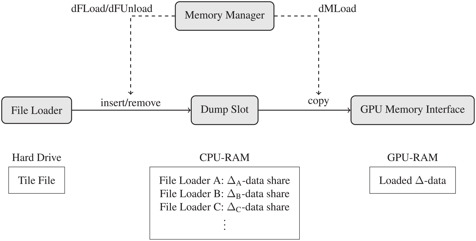
Loading the building model data.

The File Loader is responsible for the handling of a tile file. Therefore, for each tile file, a file manager instance is assigned. Its task is to open, read, and close a tile file.

The Dump Slot is an entity which manages the contents of a slot. Therefore, each slot is associated with a dump slot instance. Its task is to collect and reference all building data which belong to the area of a slot. To do so, the dump slot contains a map container in which the triangle data set is organized. Furthermore, a Boolean state of the dump slot indicates if related building data is loaded into GPU-RAM or not.

The GPU Memory Interface serves as interface to the (virtual) GPU memory.

The Memory Manager controls the instances of file loaders, dump slots, and GPU memory interfaces for the current computational unit. Besides initialization of these instances, its additional task is to decide, which slots are to be used and which of those are to be loaded into GPU to be considered in the computation process. For this purpose, the memory manager instructs all file loaders within the radius of dFLoad to load their tile file when requested by the PE. In addition to the loading command, the memory manager also sends an unload command to all file loaders that have a larger distance than dFUnload. During file loading, the file loader reads its entire tile file and forwards its data (coordinates and normal information of the triangles) to the dump slots. The radius dMLoad < dFLoad controls the active state of a slot. A slot is activated as soon as the memory manager receives a request from the PE within a radius dMLoad. The building data of the activated slot is copied to GPU-RAM. Furthermore, dedicated slots are created for regions with tall buildings which are always set to active.

Figure 7 shows an example of loaded building data considering its assignment to slots, visualized as black grid, and corresponding active states, i.e., availability of slot-wise building data in GPU memory. In the present situation, the rover is located near a boundary of a low-density tile file (red and brown buildings) and a high-density tile file (blue and steel blue buildings).

Figure 7.

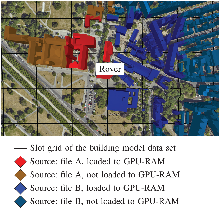
Memory management of the multipath simulator.

The memory management described above is optimized for the multipath simulation application. It loads mainly those triangles to GPU memory, which are inside a configurable sphere. As long as the rover does not leave its slot, there is no (3D building model) memory traffic at all. In case the rover moves out of its slot, a fast memory copy from CPU-RAM to GPU-RAM is required. A data transfer from secondary storage, i.e., a loading of tile files from hard disk, is rare, as relevant data are temporarily stored in the CPU-RAM. Even in the worst case scenario, when a dynamic rover is moving through an urban area at a speed of 120 km/h, there is sufficient time for the file loader to complete its loading task.

3.3. Load balancing multireceiver requests

A load balancing server is developed in order to distribute the computation load equally among the available hardware without interrupting the memory management described in the previous section.

Figure 8 shows the data flow from the PE to the multipath simulator. The multipath simulator is also accessible from outside via Internet. Hence, the simulator has to be protected against inappropriate usage. The firewall checks the validity and consistency of the incoming requests. Accepted PE requests are forwarded to the distribution server, which is the core of the load balancing mechanism. The server tracks the performance and forwards the requests to suitable computation units.

Figure 8.

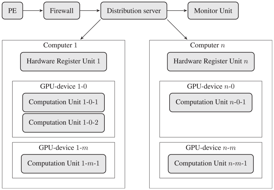
Workload distribution of the multipath simulator.

A registration message is generated by a hardware registration unit in case computer hardware should be used for the multipath simulator. Registration messages notify the distribution server that a GPU device is available. The distribution server maintains a list of all GPU devices including the corresponding GPU-RAM sizes and response times. In addition, the distribution server keeps a list of all scheduled computation units including the corresponding rover ID. When a PE request arrives at the distribution server, the server checks for any GPU device assigned to the ID of the rover. If this is not the case, a new computation unit for the rover is scheduled. In contrary, when a GPU device is assigned to a rover ID and no open request is present on that computation unit, the request is forwarded to that unit to be processed. The request is discarded if there is an open request on that computation unit, because only one request per rover is permitted.

Each computation unit has its own memory manager and is dedicated to a single graphics device. The timeout of the PEs is defined to 100 ms in order to allow them to complete its computation tasks before the start of the next epoch, assuming a data rate of 1 Hz. The processing of a request at the GPU usually requires a fraction of the time interval between two epochs. Therefore, the graphics device can be shared by multiple computation units as long as the memory of the device is sufficiently large, and the response times are short enough. If there is no GPU device assigned to the rover, a new computation unit has to be scheduled on the GPU device with minimum score. The computation units are scheduled by the hardware register units. The score takes the current utilization of the GPU hardware and CPU-RAM into account and is computed by the following equation:

Score = L + \frac{ω \sum_{i \in γ} N_{i}}{M_{γ}}

(1)

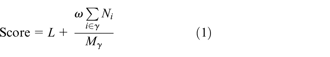
The parameter $L$ is the average latency measured at the distribution server. Initially, $L$ is set to $\infty$ , meaning that no measurement is available for the current number of computation units running on the GPU device. $N_{i}$ is the number of computation units assigned to the GPU device $i$ , which is installed at computer $γ$ , and $M_{γ}$ is the CPU-RAM memory size installed on computer $γ$ . The weight-parameter $ω$ has to be chosen suitably.

The main design goal of the load balancer is to achieve optimal scores. The score can be separated into processing performance $(L)$ and memory performance $(\sum_{i \in γ} N_{i} / M_{γ})$ . Score optimization is a multiobjective optimization problem. Hence, it is expected that the processing performance is improved by the cost of loosing memory performance. For example, the computation of the normals of the triangles of the buildings, which is needed in the ray-triangle intersection kernel, can either be accomplished while reading the model files, while loading the model data to GPU-RAM or in the kernel itself. At a first glance, both of the first two solutions put more emphasis on the processing performance, while the third approach focuses more on the memory performance. However, the situation is much more complex, since additional memory traffic leads to higher loading latencies. Therefore, a rover movement from one slot to another slot increases the risk of timeouts due to the increasing amount of memory transferred from CPU-RAM to GPU-RAM (first two solutions). In addition, using the first solution increases the load times of the model files, which in turn leads to a higher risk of timeouts when loading the files.

A monitor unit is running concurrent to the computation units. With the monitor unit, the operator is able to monitor the current multipath situation in a 3D OpenGL (Open Graphics Library) visualization. The monitor unit receives copies of the requests of a selected rover ID. The memory management of the monitor unit and the computation units differ only in the memory interface. The monitor unit uses shared OpenCL/GL memory. The programming code is completely reused. The monitor unit operates in one of two primary modes: flight mode and sky mode. In flight mode, the viewer looks down on the rover in a bird’s eye perspective and rotates around it to get an overview of the multipath situation on the ground. The sky mode creates a skyplot in the topocentric coordinate system with the rover at the center and the user looking directly at the sky.

3.4. Wall detection methodology

Wall detection is the extraction of a building model from GNSS measurements of a rover with a known location. For wall detection, it is essential to know the location of the rover as accurate as possible before starting the procedure. This can be achieved, e.g., by terrestrial tachymeter measurements.

The wall detection is divided into two sub-tasks. The first sub-task is a wall detection in the skyplot, which is partitioning of the receiver data into LOS and NLOS. Contrary to the multipath simulation approach, this has to be achieved without applying any building model.

Several techniques are provided in the literature.²⁸ In the following, we will apply an approach using the carrier-to-noise ratio (C/N₀), which is a measure for the strength of the received signal. The idea of C/N₀-LOS/NLOS-classification is that the measured C/N₀ value is compared with a reference open sky value from a calibration measurement. If the measured C/N₀ value is below a threshold, the measurement is classified as NLOS. In such a case, a building is detected in the skyplot at the certain elevation and azimuth position of the SV. A building model for the calibration location is needed, but no further building model (at the wall generation site) is required for the LOS/NLOS classification.

The second sub-task is a wall detection in the 3D environment. First, the PE processes the LOS data to compute the GNSS corrections such as clock error and atmospheric errors. Hereafter, the PE computes the code residuals of the NLOS observations, using the GNSS corrections. Our approach is based on the analysis of subsets of the NLOS code residuals.

Building walls are modeled as vertical 3D rectangular shapes, where the angle of signal incidence is equal to the angle of reflection. These significant restrictions make our approach more robust when dealing with the residuals that are affected by errors. A wall is generated by solving a two-dimensional non-linear least-squares optimization problem. 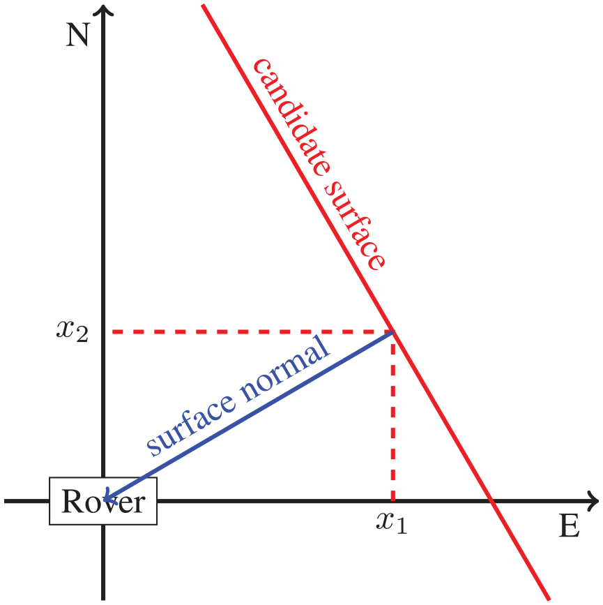As shown in Figure 9, the optimization variables ( $x_{1}$ and $x_{2}$ ) are the east and north components of a reference point in the candidate plane (height value is equal to the rovers height). The difference between the rovers coordinate and the reference point is the candidates’ normal vector. The objective of the optimization problem sums the difference between the PE residuals (measured) and the expected residuals (simulated using the surface candidate). Finally, the generated wall is either accepted, if the objective function value is below a threshold, or rejected. In the latter case, the residual sets are partitioned/merged, and the procedure is repeated.

Figure 9.

Candidate surface in the optimization problem.

Using the residuals from a simulation with the official building model, we solved the optimization problem to demonstrate the proof of concept. If our methodology works, then the objective of the optimal solution is zero or very close to zero.

Figure 10 illustrates the scenario, where the proof of concept is realized. The rover is parking in a courtyard with surrounding buildings. In the simulation, the signal of an NLOS SV is reflected at a nearby building. The reflection points are marked as a colored line in the plot. Solving the optimization problem for this proof of concept scenario produces the blue surface in Figure 10. The computed reflection surface approximates the original 3D building model. Indeed, the objective is zero, and the simulated reflection points are in the computed surface (Figure 10).

Figure 10.

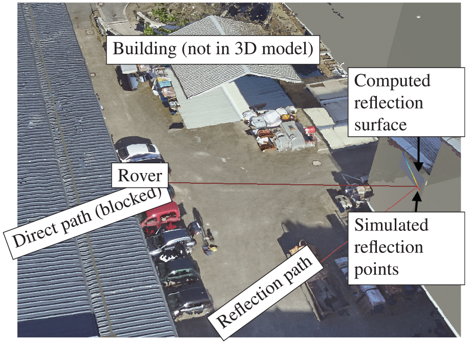
Plane computation for simulated G10 residuals.

There is no derivative of the objective available when solving the optimization problem. Thus, we analyzed a derivative-free optimization algorithm (Nelder–Mead) and several line-search and trust-region algorithms in order to find an ideal optimization algorithm (Table 1). The line-search algorithms were applied with simple backtracking (1) and backtracking using cubic approximation (2). If one of the algorithms requires derivatives, then a finite difference formula using 4 (central 4) or 2 (central 2) function evaluations is applied. The Nelder–Mead algorithm achieved the best results of our benchmark study with only 89 function calls. The number of iterations is very comparable for both finite difference formulas, so the algorithms using the central 2 formula have fewer function calls in total. The Gauss–Newton algorithm is the best line-search method. The Levenberg–Marquardt is the best trust-region method. The performance of both algorithms depends on the various configuration parameters. An unsuitable choice of these parameters leads to significant performance drops. Due to this limitation, we choose the Nelder–Mead algorithm as optimization solver.

Table 1.

Optimization algorithms applied to the proof of concept problem.

	Central 4	Central 2
Algorithm	Calls (iterations)	Calls (iterations)
Nelder–Mead	89 (46)	89 (46)
Steepest-decent 1	338,617 (33,837)	215,173 (35,291)
Steepest-decent 2	11,864 (1058)	7490 (1042)
SR1 1	420 (30)	237 (20)
SR1 2	307 (26)	208 (27)
BFGS 1	710 (69)	430 (69)
BFGS 2	329 (28)	236 (31)
Gauss–Newton 1	270 (26)	162 (26)
Gauss–Newton 2	486 (26)	270 (26)
Newton 1	607 (28)	547 (26)
Newton 2	504 (23)	374 (21)
Cauchy	11,539 (576)	2687 (167)
Dogleg	1859 (92)	913 (57)
Levenberg–Marquardt	260 (25)	156 (25)

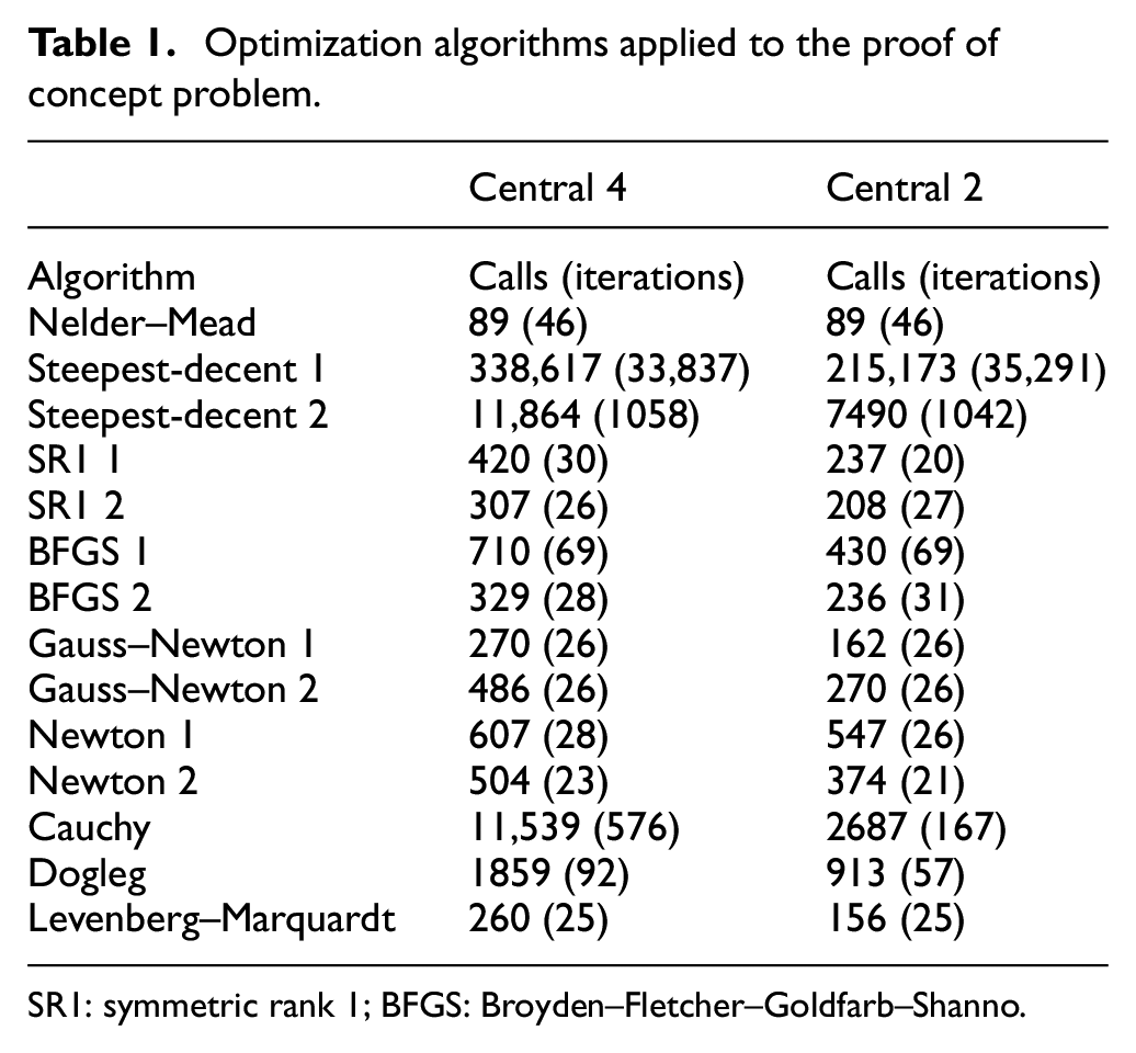
SR1: symmetric rank 1; BFGS: Broyden–Fletcher–Goldfarb–Shanno.

The robustness of the rectangular shape generator is shown by adding normal distributed noise to the simulated residuals from the proof of concept scenario and compare the optimization results with the reference solution without noise. Figure 11 shows that a standard deviation of 10 m can lead to an error of the generated wall of more than 10 m.

Figure 11.

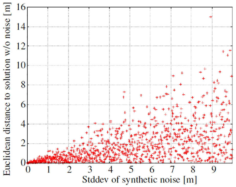
Effect of normal distributed synthetic noise to the wall location with simulated residuals.

4. Localization accuracy performance of the multipath simulator

The multipath simulator is validated by analyzing the positioning accuracy of measurements with a static rover. The measurements took place at different locations in the city of Hannover (cf. Table 2). The first measurement (data set I) was obtained in front of the main building of the Leibniz University Hannover (cf. Figure 12(a)). The data set II is placed between high office and residential buildings (cf. Figure 15(a)). In general, the positioning solutions that are computed with the multipath simulator are significantly more accurate. In the following, the positioning results are presented in detail.

Table 2.

Parameters of the data sets used in the study.

Data set	Case	SV visibility	Purpose	Location
I	Relaxed	Nearly open sky	Diffraction	Hannover University building
II	Stressed	Urban trench, small canyon	Reflection	City trench/relaxed canyon
III	Relaxed	Open sky	Wall detection, calibration	On top of a building
IV	Stressed	Urban trench, small canyon	Wall detection	Courtyard with surrounding buildings

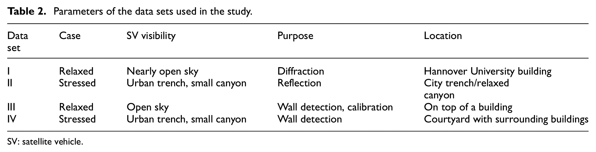
SV: satellite vehicle.

Figure 12.

Multipath simulator monitor unit in different modes for location of data set I: (a) flight mode and (b) sky mode.

The simulation state of Figure 12(a) using the sky mode is depicted in Figure 12(b). The colored lines show the trajectories of the SVs for a duration of 60 min, and the black circled lines correspond to 10° elevation angle steps. The main contributor to the multipath error in this constellation is the signal of GPS-SV G23 located behind a tower in the right side of Figure 12(b). The LOS is not obstructed at the beginning of the recording. However, after a while, the SV moves behind the tower of a neighboring building and changes its status from LOS to NLOS. At this point, the receiver is still receiving a (diffracted) signal from G23.

The diffraction analysis of G23 in the data set I is depicted in Figure 13(a). The SV G23 is not in the LOS of the receiver. The diffraction analysis tool finds a diffraction point at an edge of the roof of the tower. The signal path of the diffracted signal is longer compared to the original direct path. Hence, the multipath simulator classifies the SV as NLOS.

Figure 13.

Results from the analysis of data set I (a) diffraction analysis as result of the satellite-tower situation (for GPS satellite G23) and (b) distribution of differences versus a reference solution for the UTM east component.

The deviation to the reference coordinate of the east component computed by the PE with respect to time is plotted in Figure 13(b). The plot was obtained by post-processing the receiver data. In the first step, the receiver data were separated into intervals of 10 s. The PE computed a position for each data interval. The plot shows the difference of the PEs position to the reference position, which was computed using the complete data set (1 h). The application of the multipath simulator improves the localization quality from decimeter level to centimeter level in the data set I situation. Some individual measurements result into inaccuracies of about 0.3 m, but the most of the unfortunate situations (e.g., the G23 tower situation at time interval from 200 to 300) can be handled much better by the PE after the NLOS SVs are added to the ignore list.

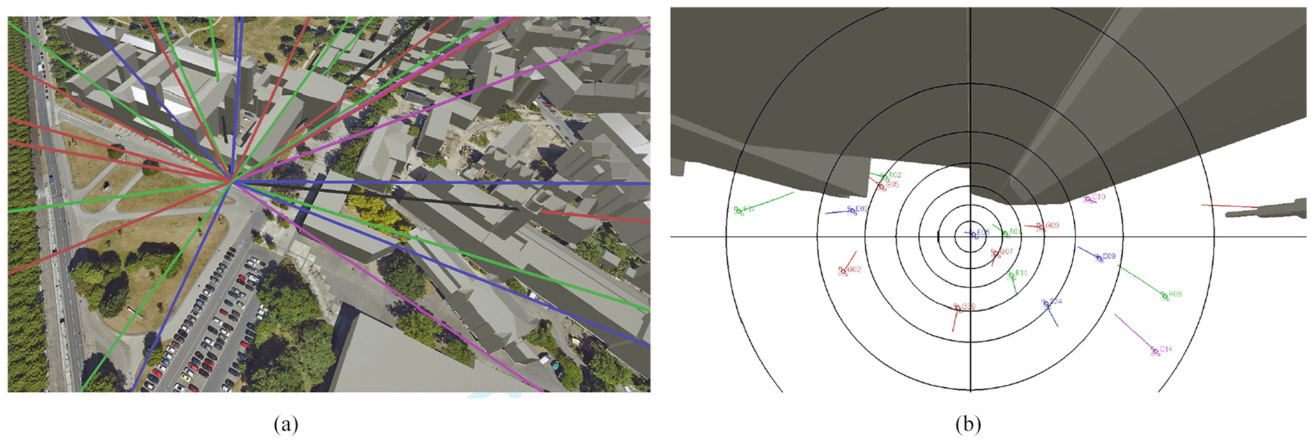
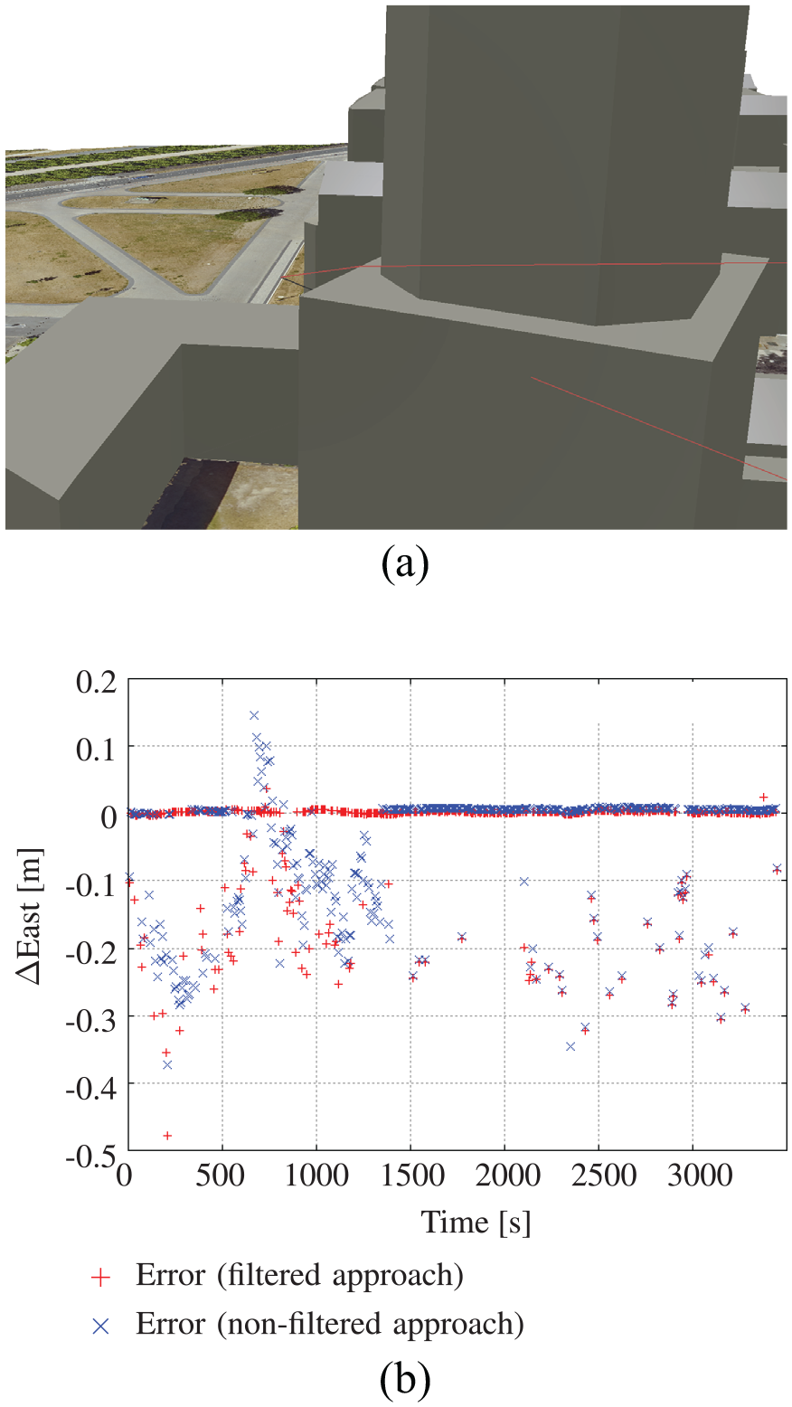
The data set II was affected by a large number of multipath errors (cf. Figure 15(a)). This scenario is the most challenging one during our analysis. The number of SVs with direct LOS was low, and the rover received many reflected and diffracted SV signals.

Figure 14 illustrates the improvement in the second scenario. Again, the multipath simulator is able to improve the localization quality significantly, but cannot reach the centimeter level in the most cases.

Figure 14.

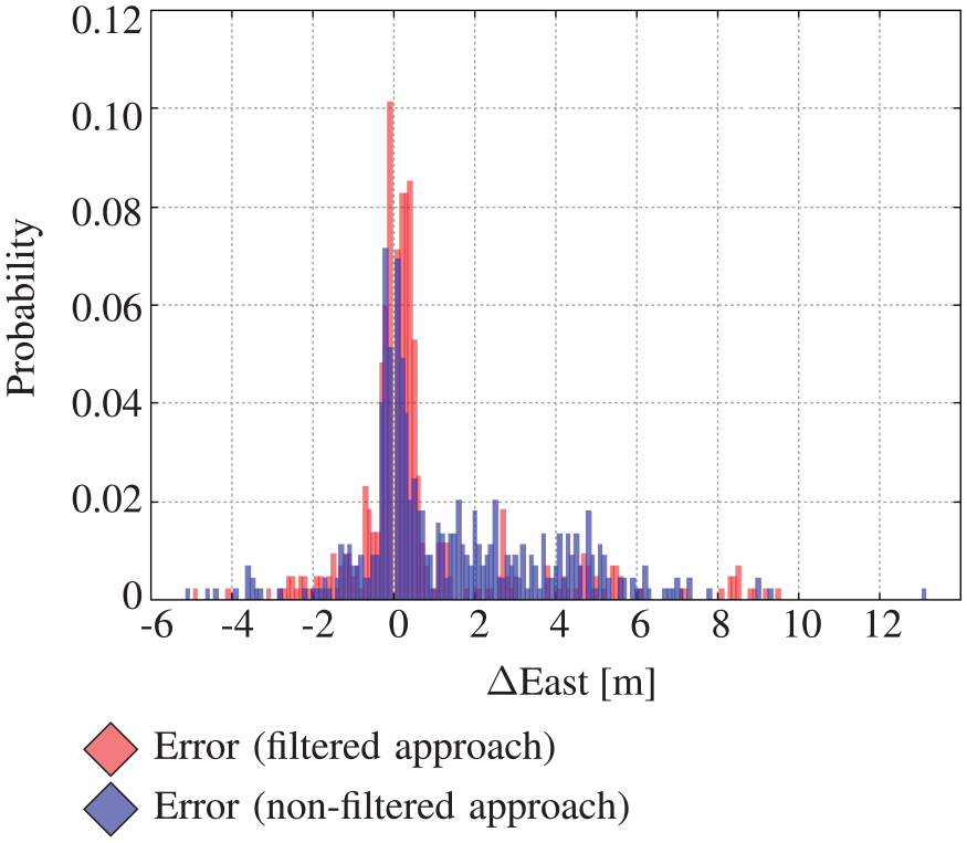
Probability of deviations in the UTM east component of the PE coordinates for the setup II.

Figure 15(b) plots the deviation to the reference coordinate of the east component computed by the PE with respect to time. The errors in the north component are very similar to the errors in the east component. Because of geometrical reasons, the errors in the height component are larger with a factor of approximately 2.5. In the time interval from 3.200 to 3.583, both methods provide relatively accurate results with errors less than a meter. Before that, in the time interval from 2.000 to 3.200, the solution using the filtered approach provides significantly better results compared to the other method. The results show that the localization solution can be more accurate, if the multipath simulator is used to pre-filter the received SV signals. Due to the small number of SVs that have a direct LOS in this very competitive environment, it is not always possible for the PE to determine an accurate position in the 10 s time span. Some position estimates (e.g., at time 1200) became even worse due to the filtering approach.

Figure 15.

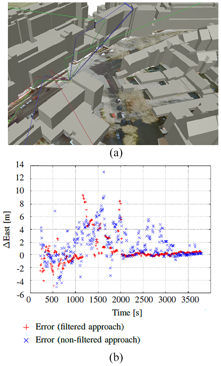
Results from the analysis of data set II (challenging satellite visibility) with (a) reflection analysis and (b) distribution of differences versus a reference solution for the UTM east component.

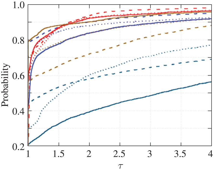
Based on performance profiles,²⁹ it is possible to find out, on which data set (I or II), the localization procedure benefited the most from the use of the multipath simulator. Figure 16 outlines the performance graphs for the data set I (red and blue) and data set II (brown and steel blue). The graph can be interpreted as follows. A higher value in the graph is better. The value at $τ = 1$ gives the proportion of localization calls, where the selected configuration (multipath on or off) was correct. The point at (2, 0.39) in the solid steel blue line (data set II, no multipath simulation) shows that 39% of the errors of the up-component are smaller than two times the corresponding error with multipath simulation. By the same way, the application of the multipath simulator reduces the error in 61% of the error measurements to less than half of the non-multipath processing.

Figure 16.

Comparison of the localization accuracy of the north (dotted), east (dashed), and up (solid) coordinate from data set I (multipath simulation: red = yes, blue = no) and II (multipath simulation: brown = yes, steel blue = no).

The blue and steel blue lines are almost always below the related red or rather brown lines. The only exceptions are the east component of the data set I measurement in the interval $1 \leq τ \leq 1.51$ and the north component in the interval $1 \leq τ \leq 1.37$ . Overall, we see that the stressed data set II profits most from the application of the multipath simulator. In particular, the height-component localization error is substantially reduced by application of the multipath simulator.

5. Response time performance of the multipath simulator

Dedicated experiments were conducted to determine important factors influencing the response time (latency) of the multipath simulator. The latency of the multipath simulation is the duration between committing a PE request and receiving the corresponding SV ignore list at the PE. The analysis splits into two parts. In the first part, the latency of single rover scenarios is analyzed. In the second part, several vehicles drive through the city at the same time to stress test the multipath simulators capability of serving multiply rovers.

5.1. Workload with a single vehicle

Figure 17 presents an example of a virtual trajectory through different environmental areas. The trajectory starts in the center of Hannover at the parking area of an industrial complex. After a short time, the vehicle appears at a main street with multiple lanes. The trajectory passes a residential area on a single lane road and leads to a city forest. Having the forest on the right and residential buildings on the left hand side, the trajectory moves away from the city center. The final part of the trajectory consists of a motorway leading through garden properties and a city forest.

Figure 17.

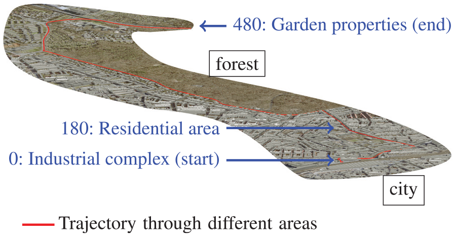
An exemplary route through different surrounding areas.

To simplify the scenario, only one single vehicle is simulated, moving with maximum permitted speed. It needs 8 min to complete the trajectory. Figure 18 shows the amount of memory, which is loaded into GPU-RAM, depending on the load radius dMLoad. Two factors affect the memory load: the type of surrounding area and the parameter dMLoad. The maximum memory amount is required for simulating multipath in inner city residential areas. The minimum amount of memory is allocated at the motorway path through the city forest, where mainly the special high building data are loaded. The loaded memory increases quadratic with dMLoad. The fit parameter for the inner city residential area with fitting function:

f (x) = a \cdot x^{2}

(2)

is $a = 271964$ with asymptotic standard error $\pm 9961 (3.663 %)$ .

Figure 18.

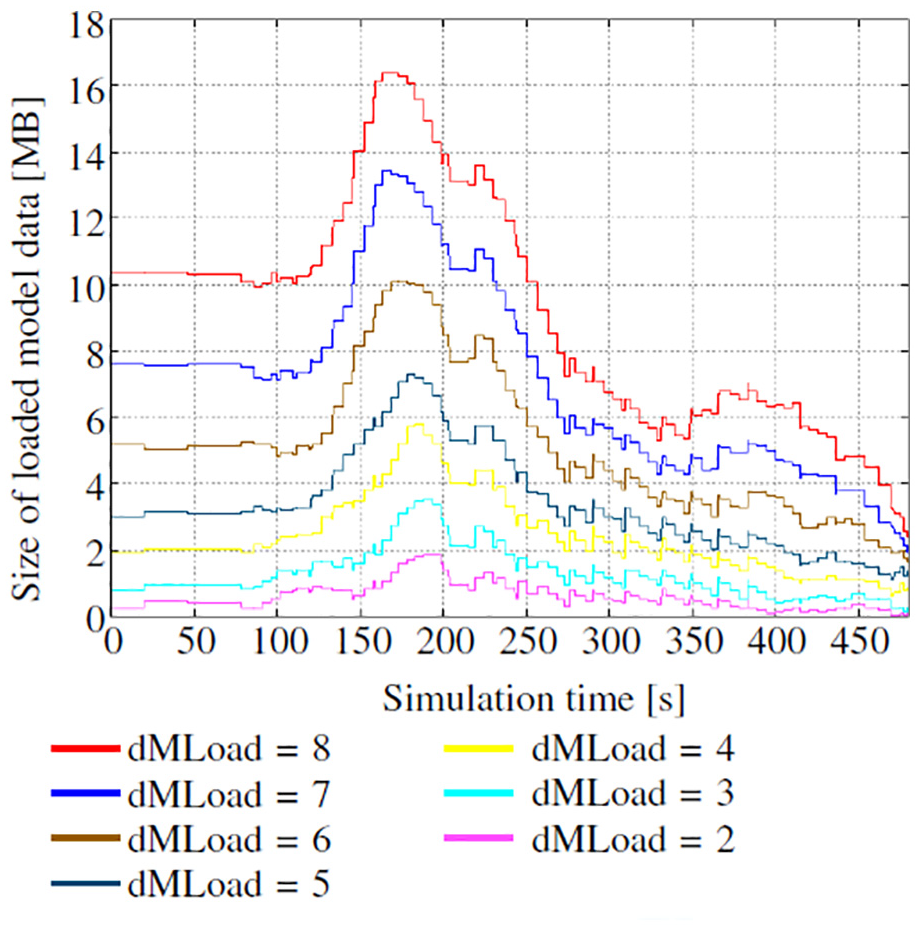
Memory loaded into GPU memory while driving on the virtual trajectory.

Figure 19 outlines the latency of the multipath simulation for a vehicle on the simulated trajectory. The reflection and diffraction analysis was omitted. For this experiment, the traffic simulator and the multipath simulator shared a Ubuntu 18.04.5 LTS, Intel Core i5-7400, GeForce GTX 1060 6 GB computer hardware setup. The epoch duration was modified in this experiment from 1 s to 100 ms in order to obtain a more detailed measurement series. The timeout parameter was set to the default value of 100 ms. Thus, the simulator processed approximately 10 requests per second.

Figure 19.

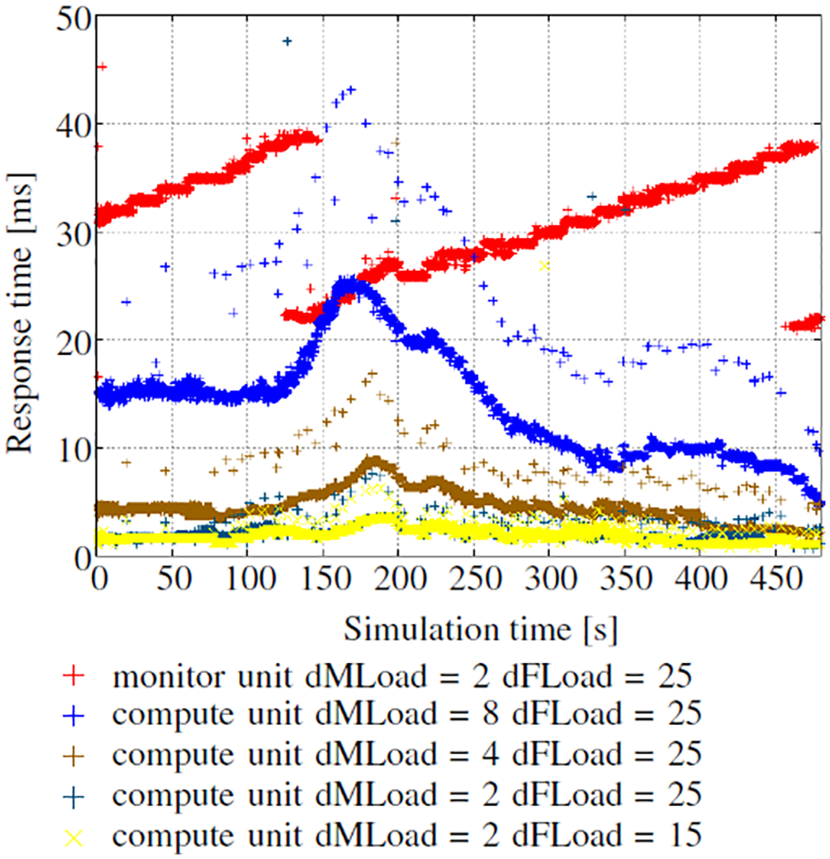
Latency measures of the multipath simulator under various environmental conditions.

There are some scattered measurements above 50 ms (approximately 1% of the $dMLoad = 8$ measurements are timeouts), which are not shown in the plot. The latencies of the computation units are very sensitive to the OpenCL parameter local size (the number of work items grouped into a work group). Hence, the optimal local size for the multipath simulator kernels had to be determined prior to our experiments. The latency of the simulator computation time is linearly depending on the loaded memory. The fit parameter for the data points with $dMLoad = 8$ with fitting function:

g (x) = a \cdot x

(3)

is a = 7.98324e−7 with asymptotic standard error ±5.738e–9 (0.7188%). Thus, the latency is mainly defined by the parameter dMLoad and the type of surrounding area. On the contrary, the percentage of timeouts is specified by the two parameters dMLoad and dFLoad, e.g., the reduction from 25 to 15 reduces the number of timeouts from 49 to 34.

The latency of the monitor unit, which is not intended to send responses back to the PE, is about one order of magnitude longer. The amount of loaded data has a minimal influence on the latency of the monitor unit. The main contributing factor here is the synchronization of the request thread and the visualization thread, because the visualization thread has to finish its current drawing work before the request thread is allowed to manipulate the memory.

5.2. Workloads with several vehicles

The generation of realistic rover movements in order to analyze the multipath simulator is challenging. The rovers have to move with appropriate velocities through the road network of the city. In addition, the rovers are not allowed to jump from one place to another and need to be distributed in a realistic manner. It is very expensive and time-consuming to perform the latency stress test with real rovers. Thus, we decided to apply the Simulation of Urban MObility (SUMO) traffic simulator³⁰ to generate realistic rover movement. The road network of the traffic simulator is created based on the OpenStreetMap data. Periodic requests were send in real-time from the PE to the multipath simulator based on the vehicle trajectories from the traffic simulator.

The nature of the surrounding area, respectively, the GPU memory, was discussed in the previous section as one of the most important factors affecting performance. Figure 20 depicts the required GPU memory $(dMLoad = 8)$ in Hannover (given in MiB, i.e., mebibyte). The map was generated by traveling along all roads in the range of the 3D building data set. The simulated trajectory of the previous section is marked as a solid black line. The area that is marked in the map is potentially the most challenging location in Hannover for this kind of performance experiments. Each computation unit has its own memory manager. Therefore, an uneven distribution of the rovers across the whole city would not result into an extreme scenario. The most challenging scenario would be, if the vehicles are concentrated at memory intense areas. Therefore, the traffic simulator is restricted to the marked area of Figure 20.

Figure 20.

Memory loaded to GPU memory in the city of Hannover.

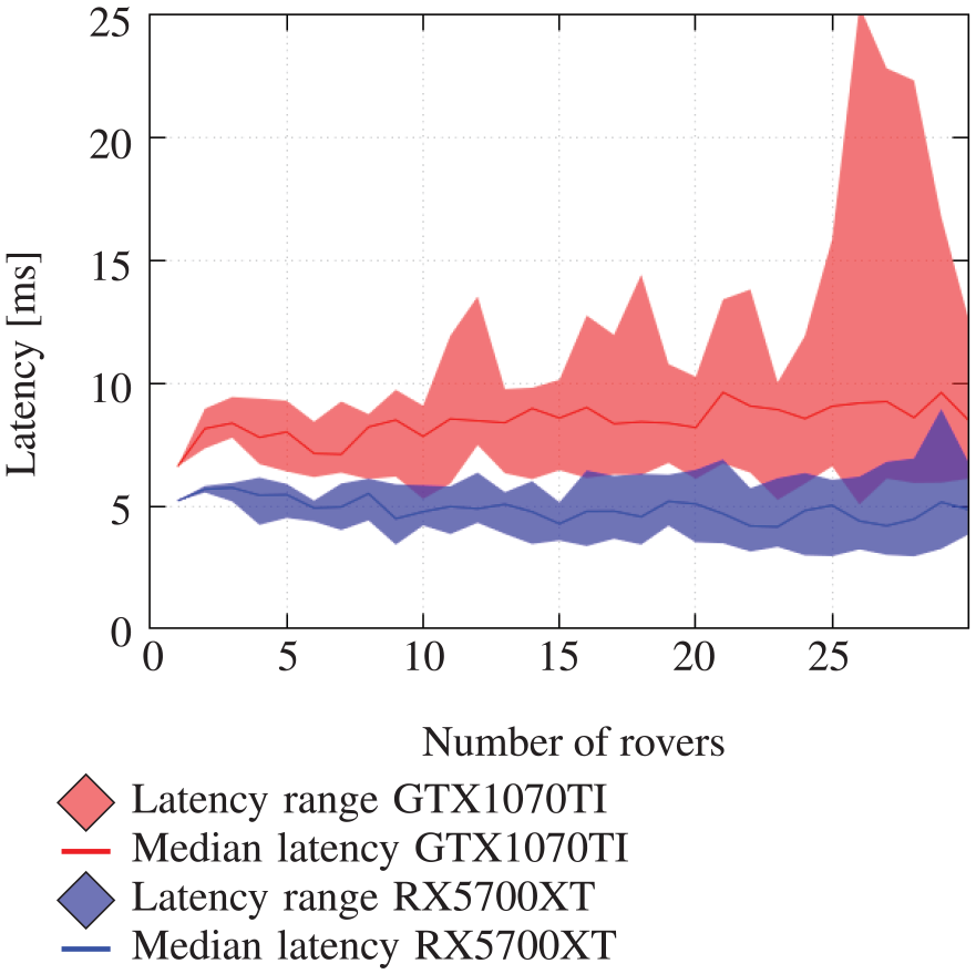
Figure 21 shows the average response times of the multipath simulator for various rover counts on two distinct hardware configurations. Table 3 lists further details on the individual configurations used. The GTX1070TI configuration is Windows 8.1 Pro, Intel Core i7-8700, GeForce GTX 1070 Ti and the RX5700XT configuration is Windows 10 Pro, AMD Ryzen 7 2700, AMD Radeon RX 5700 XT. Both systems are equipped with 16 GB CPU-RAM. The RX5700XT configuration performs better for all rover counts. Often, all RX5700XT rovers have lower latencies than the best performing GTX1070TI rover. For example, if five rovers travel through the memory intense area, the performance of all computation units is less than 5.9 ms in average on the RX5700XT configuration. With the GTX1070TI configuration, all computation units perform with more than 6.4 ms.

Figure 21.

Rover count–dependent response time performance of the multipath simulator.

Table 3.

Summary of the workload analysis with different GPUs and same processing strategy.

Hardware			Operating system	Median latency (ms)
Processor	GPU	CPU-RAM
Intel Core i7	GeForce GTX1070 Ti	16	Windows 8.1 Pro	8
AMD Ryzen 7 2700	AMD Radeon XT 5700	16	Windows 10 Pro	5

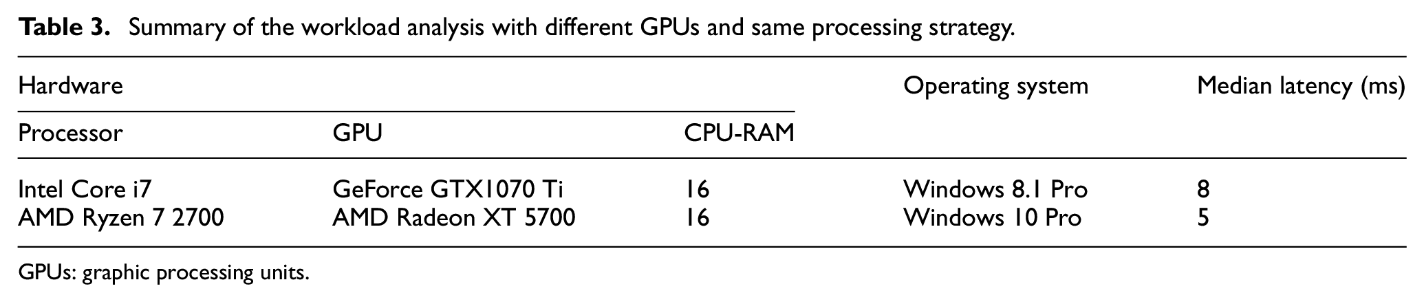
GPUs: graphic processing units.

The number of rovers simulated on a GPU device affects the simulators’ performance marginally. The RX5700XT performs with approximately 5 ms, and the GTX1070TI performs with approximately 8 ms for all rover counts. However, there are some outliers on the GTX1070TI, which perform substantially worse than the other compute units. The overall conclusion is that the multipath simulator is able to meet the real-time requirements of our use case with the provided hardware as long as the rover count is not exceeding 30 compute units. In both hardware setups, we have 16 GB CPU-RAM, which is fully used in the scenario of 30 compute units. In our studies, we found that the simulator can become unstable (graphics driver timeout crash or CPU-RAM error) if more than 25 compute units have to be processed on the RX5700XT or GTX1070TI. In practice, we would therefore limit the number of rovers on each hardware to avoid such situations or reject clients if the available hardware is not sufficiently large enough.

The performance of the simulator in a multi-GPU environment was analyzed having 50 rovers moving through the scene. The simulation was executed on the RX5700XT and GTX1070TI configurations. Figure 22 depicts the average performance of the computation units. The load balancer scheduled 25 computation units on the RX5700XT and 25 computation units on the GTX1070TI. The corresponding latency ranges in Figure 21 are 2.96–6.06 ms and 6.61–15.85 ms. The performance values of the multi-GPU experiment fit to the corresponding latency ranges. Thus, the load balancer is able to distribute the workload without significant additional performance costs.

Figure 22.

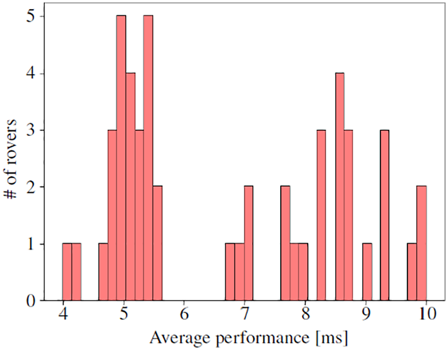
Multipath simulator latencies with 50 rovers running on GTX1070Ti and RX5700XT devices.

The experiments verify the hypothesis, that the number of rovers does not affect the latency of the multipath simulator. The experiments were carried out with up to 50 rovers, and the multipath simulator completes its task reliable without significantly missing the real-time requirements. There might be some limitations in the experiments: rovers are virtual and not in the real down town traffic, the distribution of the rover is not realistic (stress test scenario where all rovers are located at the most challenging area), and only 50 rovers are simulated and not thousands of rovers. We suggest to treat the first two limitations by equipping vehicles, which are moving through the entire city anyway such as mail cars or buses for public transport. An increase of the rover count from 50 to thousands of rovers involves considerable expense. It is necessary to provide considerably more hardware for simulation execution for thousands of virtual rovers. Experiments with thousands of non-virtual rovers are currently not possible because this requires access to the vehicle position of thousands of vehicles in the city in real-time.

6. Application of wall detection

The two sub-steps of the wall detection methodology are applied to the data set IV from Table 2, whereby the GNSS equipment of the rover was previously calibrated (data set III).

6.1. Skyplot building detection using the carrier-to-noise density ratio

The calibration experiment (data set III) was conducted on the roof of a university building. The 3D model from the Hannover data set was extended by a more accurate model derived from a terrestrial laser scan, and refined by accurate modeling the GNSS signal reception conditions. Hence, the building model is more accurate at this site.

Figure 23 shows the C/N₀ measurements after application of a Butterworth filter with respect to the SV elevations. Red points are observations, where the rover location, SV location, and the reference 3D model would lead to an LOS signal. The NLOS signals in the reference 3D model are blue points. This scenario is equal to an open sky scenario, as there is no blocking building below a zenith angle of 75°. To distinguish between LOS and NLOS without a building model, we suggest to introduce a function (threshold) and classify the measurements above the threshold as LOS and the measurements below the threshold as NLOS.

Figure 23.

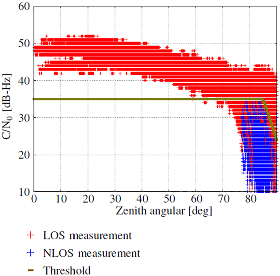
Carrier-to-noise ratio measurements of Galileo $L_{1}$ signal in the roof scenario.

Figure 24 shows the classification results of our strategy (with a simple linear spline) compared to the results using the refined 3D building model. The viewer is at the rovers’ antenna position and looks into the direction of a roof structure. Red dots show the SV positions, where the LOS/NLOS classification with the simple strategy is consistent to the LOS/NLOS classification of the 3D model. Blue dots show the SV positions, where the measured C/N₀ is below the threshold, but the building model yields to an LOS situation. The yellow dots show the SV positions, where the C/N₀ is above the threshold, but the building model yields to an NLOS situation. We see errors of type 1 at the edges of the roof construction and errors of type 2 at the corner of the roof construction. Since, the signal progressions are modeled as rays in this publication, an explanation of the phenomena (Fresnel zone model) is out of scope. We should also mention some type 2 error measurements at the center of the roof construction, which suggest that our simple approach should not be applied to zenithal observations, i.e., close to 88° zenith angle. In practice, we compute the threshold for every SV, every signal and every hardware setup (antenna and receiver) in an open sky scenario and use the Lagrange polynomials for threshold interpolation.

Figure 24.

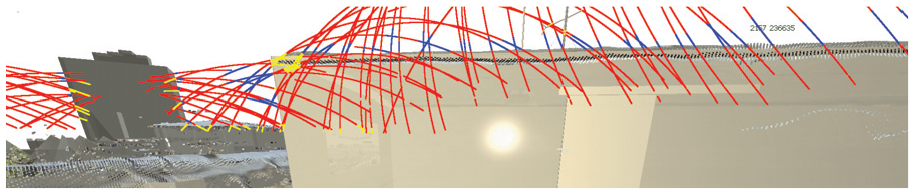
Wall detection in skyplot (red: classification correct, blue: error type 1, and yellow: error type 2).

6.2. 3D rectangular shape generation

The second sub-task is the detection of 3D rectangular shapes, which represent walls in the 3D model.

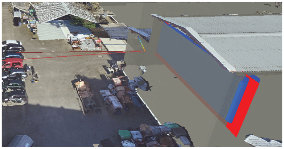
Figure 25 shows the detected wall, when the residuals of one SV (G10) calculated by the PE are used. The detected wall is at the roof of a building, which is not part of the 3D model. The building is visible due to the orthophotos, which were implemented into the monitor unit.

Figure 25.

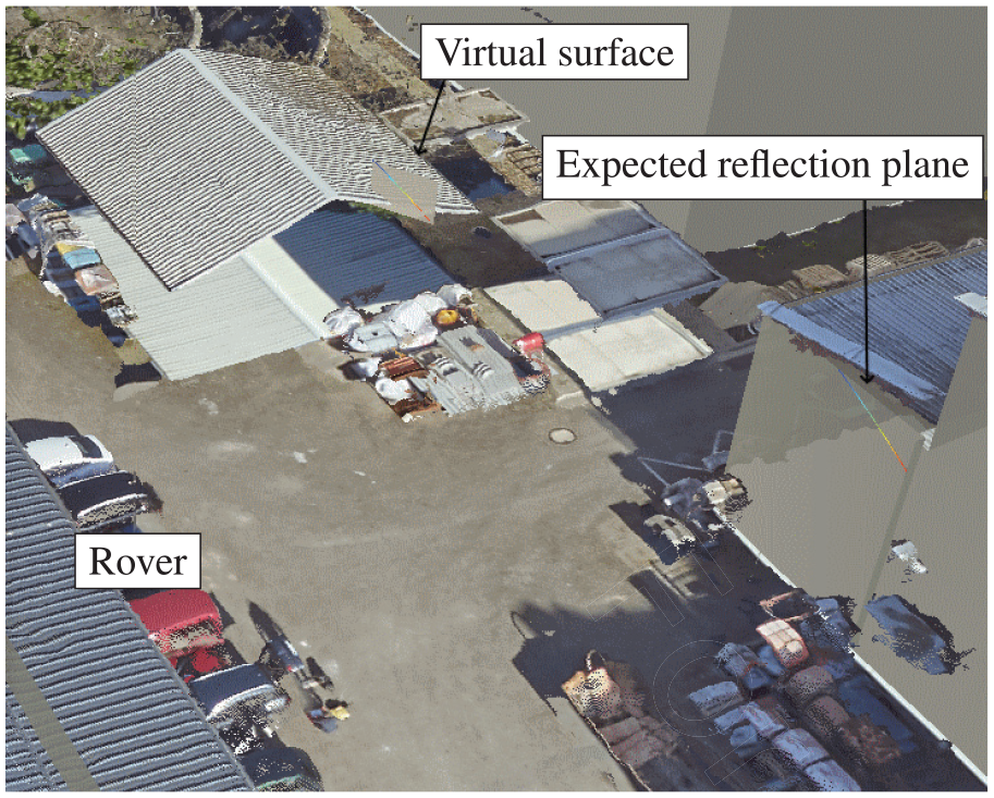
Wall detection result using a single SV.

The residuals of the G10 virtual surface situation are plotted in Figure 26. The residuals from the virtual plane reflection fit better to the PE output than the residuals of the reflection path from the building model. It is not possible to state which of the two reflection paths (virtual or building model) is the real reflection path. It is also possible that none of them is the real signal path. According to the results of the studies, we conclude that for static rovers, the detection/identification of walls can only be meaningful and sufficient if the residuals of more than a single satellite are processed by the wall detector.

Figure 26.

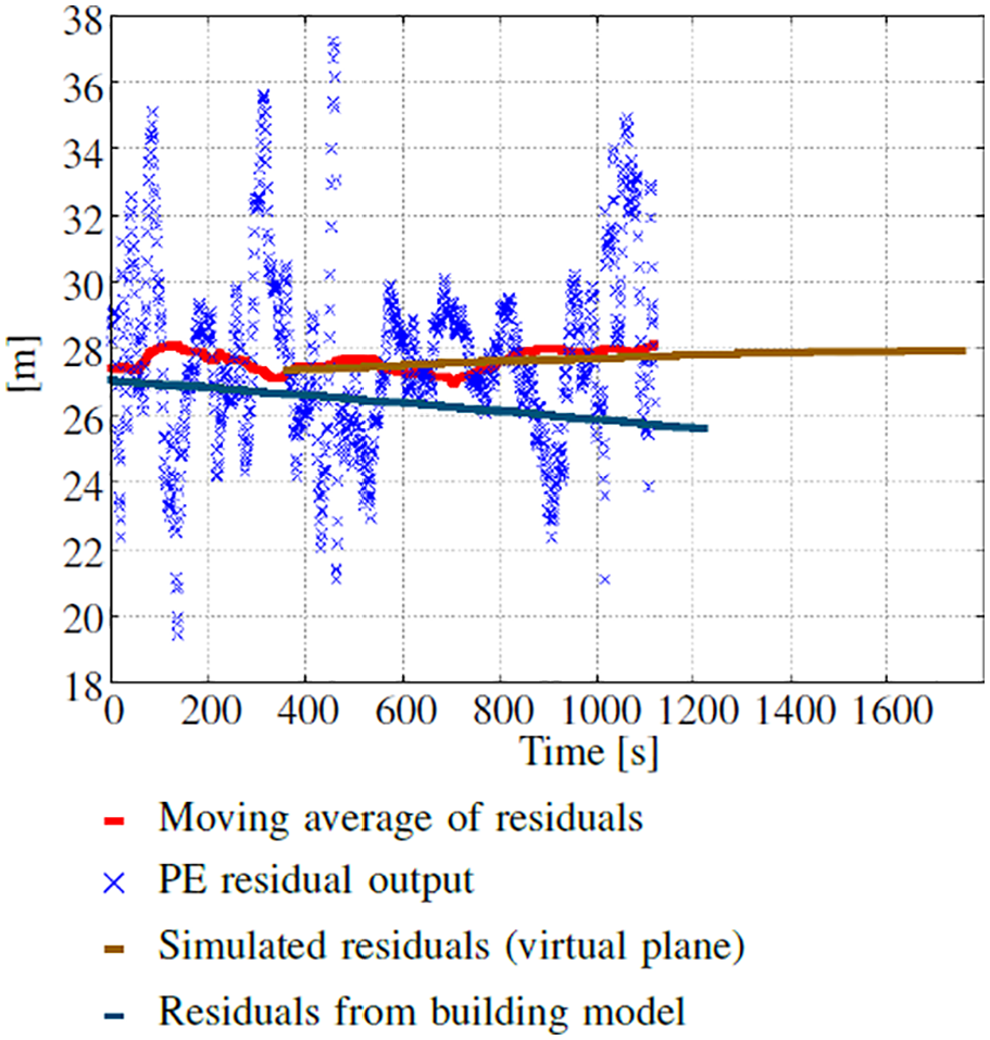
Residuals of the G10 virtual surface situation.

The red plane in Figure 27 is the optimization result when residuals from two different SVs are used. Compared to the wall in the 3D model, we can see a deviation of about 1 m. It seems that the multipath simulator suggested a wrong part of the building as the main reflector for the signal. There are several blue planes in front of and behind the red plane. The blue planes are detected walls using only sub-sets of the original residual data set. Two types of split routines are implemented, such as front-back and left-right-up-down, as well as a merge routine to separate the data set. The blue planes result from the front-back split routine.

Figure 27.

Wall detection result using two SVs.

7. Conclusion

A GNSS multipath simulator for real-time applications in autonomous driving and a wall detector for building model generation are presented.

The multipath simulator meets the real-time requirements and is able to improve the localization accuracy, in particular under urban condition with potentially high multipath impact. The computation core of the multipath simulator is designed for processing on GPU hardware. A memory management provides fast and efficient access to the building model data. A load balancer distributes the workload even to all available hardware. The improvement of the localization accuracy is shown by analyzing two GNSS data sets in urban and city areas. It is shown that the multipath simulator improves the localization accuracy especially in areas with very dense building development. The latency of the multipath simulator is analyzed with stress tests including up to 50 rovers in the down town area. The latency of the multipath simulator shows linear dependence on the GPU memory consumption of the building model. The latency is almost constant with regard to the number of rovers processed on the hardware.

A novel wall detection method based on GNSS signal analysis is presented. The approach is able to detect walls when the signals from more than one SV are reflected from the wall.

The size of the CPU-RAM was identified as a bottleneck when processing a large number of rover requests. A hardware upgrade could solve the challenge. Another way to handle the bottleneck is an alternative implementation that includes a shared CPU-RAM for all computation units running on a computer. Weighing the advantages and disadvantages of such an alternative approach will be examined as part of future research.

Static rover experiments were performed to analyze the localization accuracy of the multipath simulator. We found that the PE is not able to determine an accurate rover position under certain circumstances. The next step is to conduct kinematic experiments in areas with high buildings to perform detailed multipath analysis and improve the positioning performance. Based on the results of our kinematic experiments, we plan to modify the multipath simulator to provide more detailed information to correct for positioning errors in difficult urban areas.

Footnotes

Funding

The author(s) disclosed receipt of the following financial support for the research, authorship, and/or publication of this article: This project was funded by the Federal Ministry for Economic Affairs and Climate Action (BMWK) based on a resolution of the German Bundestag and supervised by TÜV-Rheinland (PT-TÜV) under the grants 19A20002A-C.

ORCID iD

Marcus O’Connor

Author biographies

Marcus O’Connor received his MSc in mathematics at the Leibniz University Hannover (LUH). He is currently a PhD candidate at LUH and works at Geo++ GmbH in Garbsen as a research assistant and software developer. His research interests cover simulation and modeling of urban environments, real-time simulations, and integration of graphics hardware into simulation computations.

Tobias Kersten received his Dr.-Ing. in geodesy and geoinformatics from Leibniz University Hannover (LUH) in 2014. Currently, he is working as a scientific associate and project coordinator in the positioning and navigation group of the Institut für Erdmessung (IfE) at LUH. His interests and work cover Precise Point Positioning, stochastic modeling of receiver antenna calibration for code and carrier phase, signal interference phenomena, and low-cost GNSS for geoscience and urban applications.

Christian Skupin received the Dipl.-Ing and Dr.-Ing (PhD) degrees in telecommunications engineering from Leibniz University Hannover (LUH) in 2008 and 2013, respectively. In 2011, he joined the Robert Bosch GmbH and is now with the Distributed Perception and Positioning group as part of Bosch Corporate Research. His research interest lies in the field of digital signal processing with applications in communications and navigation with a current emphasis in GNSS for automotive localization in urban areas.

Fabian Ruwisch received his BSc and MSc degree in geodesy and geoinformatics from LUH in 2016 and 2019, respectively. Currently, he is a PhD candidate in the positioning and navigation group of the IfE at LUH. His research interests include GNSS multipath modeling as well as the Kalman filtering for relative positioning in urban areas.

Le Ren received his Dr.-Ing. in geodesy and geoinformatics from Leibniz University Hannover (LUH) in 2020. Currently, he is working as a GNSS Specialist at Geo++. His interests and work cover PPP and PPP-RTK, LEO-satellite orbit determination, ionospheric scintillation, GNSS Software testing, and quality assurance.

Temmo Wübbena received his PhD in physics from Leibniz University Hannover (LUH) in 2013. He joined Geo++ in 2013 where he has been involved in the development of multiple GNSS augmentation services, including QZSS CLAS. He is currently overseeing business development as well as research projects as managing director at Geo++. His scientific interests and work cover satellite navigation augmentation as well as quantum sensing.

Steffen Schön is a professor for positioning and navigation at IfE since 2006. His research interests are the correction and assessment of systematic errors in GNSS, absolute antenna calibration, use of miniaturized atomic clocks for navigation, and improved stochastic models for GNSS observations based on turbulence theory. He is also currently the spokesman of the DFG research training group integrity and collaboration in dynamic sensor networks (i.c.sens) working on interval mathematics for integrity and collaborative navigation.

References

Sun

Zhai

Qin

Crowd navigation in an unknown and dynamic environment based on deep reinforcement learning. IEEE Access 2019; 7: 109544–109554.

Butt

Riaz

Mehmood

, et al. REEEC-AGENT: human driver cognition and emotions-inspired rear-end collision avoidance method for autonomous vehicles. Simulation 2021; 97: 601–617.

Singh

Bera

Chatti

A real-time obstacle avoidance and path tracking strategy for a mobile robot using machine-learning and vision-based approach. Simulation 2022; 98: 789–805.

Sun

Xue

Zhang

. Rear-end collision detection based on GNSS/compass fusion and adaptive neuro fuzzy inference system. In: 2017 Forum on Cooperative Positioning and Service, Harbin, China, 19–21 May 2017, pp. 273–277. New York: IEEE.

Levinson

Montemerlo

Thrun

Map-based precision vehicle localization in urban environments. In Robotics: science and systems III (ed. Wolfram Burgard

Stachniss

), Georgia Institute of Technology, Atlanta, GA, 27–30 June 2007. Cambridge, MA: MIT Press.

Kuutti

Fallah

Katsaros

, et al. A survey of the state-of-the-art localization techniques and their potentials for autonomous vehicle applications. IEEE Internet Things 2018; 5: 829–846.

Kamijo

Hsu

LT.

Autonomous vehicle technologies: localization and mapping. IEICE ESS Fundam Rev 2015; 9: 131–141.

Kumar

Petovello

. A novel GNSS positioning technique for improved accuracy in urban canyon scenarios using 3D city model. In: Proceedings of the 27th International Technical Meeting of the Satellite Division of The Institute of Navigation (ION GNSS + 2014), 8–12 September 2014, pp. 2139–2148. Tampa, FL: Tampa Convention Center. https://www.ion.org/publications/abstract.cfm?articleID=12508

Bétaille

Miquel

Godan

, et al. 3D-city-model-aided GNSS accurate positioning with integrity provision using simplified geometry of buildings. In: European navigation conference (ENC), Bordeaux, 8–10 April 2015, p. 6. https://hal.archives-ouvertes.fr/hal-01206096/document

10.

Hsu

Tokura

Kubo

, et al. Multiple faulty GNSS measurement exclusion based on consistency check in urban canyons. IEEE Sens J 2017; 17: 1909–1917.

11.

Wen

Zhang

Hsu

. Exclusion of GNSS NLOS receptions caused by dynamic objects in heavy traffic urban scenarios using real-time 3D point cloud: an approach without 3D maps. In: 2018 IEEE/ION position, location and navigation symposium (PLANS), Monterey, CA, 23–26 April 2018. New York: IEEE.

12.

Hsu

Kamijo

. Sensor integration of 3D map aided GNSS and smartphone PDR in urban canyon with dense foliage. In: 2016 IEEE/ION position, location and navigation symposium (PLANS), Savannah, GA, 11–14 April 2016. New York: IEEE.

13.

Bradbury

Ziebart

Cross

, et al. Code multipath modelling in the urban environment using large virtual reality city models: determining the local environment. J Navigation 2006; 60: 95–105.

14.

Groves

Wang

Adjrad

, et al. GNSS shadow matching: the challenges ahead. In: Proceedings of the 28th ION GNSS+ 2015, 14–18 September 2015, Tampa, FL, pp. 2421–2443. Tampa, FL: Tampa Convention Center.

15.

Miura

Hisaka

Kamijo

GPS multipath detection and rectification using 3D maps. In: 16th international IEEE conference on intelligent transportation systems (ITSC 2013), The Hague, 6–9 October 2013. New York: IEEE.

16.

Zhang

, et al. GNSS RUMS: GNSS realistic urban multiagent simulator for collaborative positioning research. Remote Sens 2021; 13: 544.

17.

Icking

Ruwisch

Schön

Multipath characterization using ray-tracing in urban trenches. In: Scientific assembly of the International Association of Geodesy (IAG), Beijing, China, 28 June–2 July 2021.

18.

Wang

Groves

Ziebart

. Urban positioning on a smartphone: real-time shadow matching using GNSS and 3D city models. In: Proceedings of the 26th ION GNSS+ 2013, 16–20 September 2013, Nashville, TN pp. 1606–1619. https://www.ion.org/publications/abstract.cfm?articleID=11339

19.

Wang

Groves

Ziebart

MK.

Multi-constellation GNSS performance evaluation for urban canyons using large virtual reality city models. J Navigation 2012; 65: 459–476.

20.

van Diggelen

. End game for urban GNSS: Google’s use of 3D building models. Inside GNSS, 2021. https://insidegnss.com/end-game-for-urban-gnss-googles-use-of-3d-building-models/

21.

Voelsen

Schachtschneider

Brenner

Classification and change detection in mobile mapping LiDAR point clouds. PFG: J Photogramm Remote Sens Geoinf Sci 2021; 89: 195–207.

22.

Zou

Sester

Incremental map refinement of building information using LiDAR point clouds. Int Arch Photogramm Remote Sens Spatial Inf Sci 2021; XLIII-B2-2021: 277–282.

23.

Oconnor

Ruwisch

Kersten

, et al. Low-latency GNSS multipath simulator for real-time applications in autonomous driving. In: 2021 IEEE/ACM 25th international symposium on distributed simulation and real time applications (DS-RT), Valencia, 27–29 September 2021. New York: IEEE.

24.

Ali

Gupta

Sharma

YC.

A brief overview of wireless cellular networks: LTE HetNets perspective. Int J Latest Trends Eng Technol 2018; 10: 96–104.

25.

Möller

Trumbore

Fast, minimum storage ray-triangle intersection. J Graph Tools 1997; 2: 21–28.

26.

Open Geodata. Digitales 3D-Stadtmodell (City GML 2.0). Servicecenter Geoinformation, 2021. https://opengeodata-hannover.de

27.

Kreitlow

Brettschneider

Jahn

, et al. ETRS89/UTM—the reference system change and its impact on geodata usage. Kartogr Nachr 2010; 60: 14. https://www.lgln.niedersachsen.de/download/126849/KN_2010_Heft_4.pdf

28.

Lines

Basiri

3D map creation using crowdsourced GNSS data. Comput Environ Urban 2021; 89: 101671.

29.

Dolan

Moré

JJ.

Benchmarking optimization software with performance profiles. Math Program 2002; 91: 201–213.

30.

Krajzewicz

Hertkorn

Rössel

, et al. SUMO (Simulation of Urban MObility)—an open-source traffic simulation. In: Proceedings of the 4th middle east symposium on simulation and modelling (MESM20002), Sharjah, September 2002, pp. 183–187. Berlin-Adlershof: Institute of Transport Research.

Low-latency GNSS multipath simulation and building wall detection in urban environments

Abstract

Keywords

1. Introduction

2. Multipath simulator and wall detector

3. Implementation details

3.1. General GPU accelerated computation approach

3.2. Memory management of the multipath simulator

3.3. Load balancing multireceiver requests

3.4. Wall detection methodology

4. Localization accuracy performance of the multipath simulator

5. Response time performance of the multipath simulator

5.1. Workload with a single vehicle

5.2. Workloads with several vehicles

6. Application of wall detection

6.1. Skyplot building detection using the carrier-to-noise density ratio

6.2. 3D rectangular shape generation

7. Conclusion

Footnotes

Funding

ORCID iD

Author biographies

References