Sage Journals: Discover world-class research

Abstract

According to state-of-the-art research, mobile network simulation is preferred over real testbeds, especially to evaluate communication protocols used in Opportunistic Networks (OppNet) or Mobile Ad hoc NETworks (MANET). The main reason behind it is the difficulty of performing experiments in real scenarios. However, in a simulation, a mobility model is required to define users’ mobility patterns. Trace-based models can be used for this purpose, but they are difficult to obtain, and they are not flexible or scalable. Another option is TRAce-based ProbabILiStic (TRAILS). TRAILS mimics the spatial dependency, geographic restrictions, and temporal dependency from real scenarios. In addition, with TRAILS, it is possible to scale the number of mobile users and simulation time. In this paper, we dive into the algorithms used by TRAILS to generate mobility graphs from real scenarios and simulate human mobility. In addition, we compare mobility metrics of TRAILS simulations, real traces, and another synthetic mobility model such as Small Worlds in Motion (SWIM). Finally, we analyze the performance of an implementation of the TRAILS model in computation time and memory consumption. We observed that TRAILS simulations represent the interaction among users of real scenarios with higher accuracy than SWIM simulations. Furthermore, we found that a simulation with TRAILS requires less computation time than a simulation with real traces and that a TRAILS graph consumes less memory than traces.

Keywords

Mobility model social network virtual society simulations simulation analysis spatial interaction model agent-based model

1. Introduction

There is an increasing interest in the development of mobile network protocols,¹ and there are two possible methodologies to evaluate the performance of new protocols. The first methodology is real testbeds, and the second is through simulation. Testbeds can mirror real scenarios closer than simulations, but simulations are easier to scale and repeat.² In consequence, simulators are preferred in the evaluation of Opportunistic Networks (OppNet) and Mobile Ad hoc NETworks (MANET) protocols.³

Mobility models have a major effect on the protocol performance of wireless networks. Therefore, a mobility model should mimic the users’ movements of the targeted real scenario. Otherwise, the observations made from the simulation may be incorrect.⁴ In addition, there are recent efforts to increase the accuracy of Wireless Sensor Networks (WSN) in combination with cloud computing, such as SensorCloudSim.⁵ In consequence, it is important to also improve the accuracy in scenarios where sensors are attached to humans or other mobile entities using a scalable mobility model capable of representing the movement of real users.

Mobile network protocols have an extensive range of applications. For example, they are used in WSNs to monitor sea birds⁶ and opportunistic networks for workers in disaster recovery scenes.⁷ In the mentioned applications and many others, mobility plays a significant role in the efficiency of the protocol.⁸

Mobility models can be trace-based models or synthetic models. Trace-based models represent real users’ movement on specific scenarios, but they are difficult to obtain, and recorded scenarios available in public databases are limited. However, synthetic models are flexible and scalable, but their statistical results may differ from real scenarios depending on the model.⁹

Usually, mobility models are employed to represent human mobility, which is characterized by different aspects. People usually are more attracted to visit the same places every day, but they also take irregular trips.¹⁰ People behave as a social network with a high level of clustering.¹¹ Consequently, to represent a human social network, we need a model that can capture three characteristics from traces.¹² Those characteristics are spatial dependency, temporal dependency, and geographic restrictions.¹³ Pure-random synthetic models such as Random WayPoint (RWP) do not capture any of these characteristics.¹⁴ However, there are mobility models that capture one or more of the mentioned characteristics. For example, SWIM captures spatial and temporal dependency by exploiting human tendency to gather in popular locations.¹⁵ Another example is TRAce-based ProbabILiStic (TRAILS), which captures all three characteristics by extracting information from real traces. The TRAILS model presented in this paper builds upon the paper “TRAILS-A Trace-Based Probabilistic Mobility Model.”¹⁶ Our work enhances the previous algorithms by considering the changes of human routines over time, as explained in section 3.1.

In this paper, we explain in section 2 the concepts behind mobile networks and mobility models. Then, in section 3, we describe the TRAILS model and its algorithms. In section 4.1, we present three different scenarios that represent the mobility of pedestrians and vehicles. In sections 4.2 and 4.3, we portray the properties of users’ contacts of TRAILS, SWIM, and traces. In section 4.4, we analyze the performance of TRAILS algorithms, and we describe the effects of varying the simulation time and the number of users in TRAILS simulations. In section 4.5, we present the effects of TRAILS, SWIM, and traces of real scenarios in the performance of OppNet protocols. Finally, in section 5, we summarize our findings.

2. Related work

Mobility models are widely used in the research of mobile networks,¹⁷ and TRAILS is a mobility model that mimics users’ statistical behavior in real scenarios. That is why, in this section, we present an overview of mobile networks and we review the key factors of synthetic and trace-based mobility models.

2.1. Mobile networks

There are two large categories of decentralized mobile networks. The first category is MANET, and the second one is OppNet. In the past decade, many researchers have studied the effects of mobility models in both categories.¹⁸ MANET is a set of mobile users forming a network without a predefined infrastructure where a user defines a communication path before sending a message.¹⁹ However, OppNet is a delay-tolerant mobile network where users forward messaged without an established end-to-end communication path.²⁰

Mobile network protocols have a different performance under different scenarios. Therefore, we should evaluate those protocols under realistic conditions, such as a mobility model capable of representing human behavior in a reasonable way.⁴

To measure the performance of mobile network protocols, we can use the following metrics: end-to-end delay, that describes the mean time of a message since its creation until it reaches its destination²¹ and packet delivery ratio, that represents the relation of the number of packets transmitted versus the number of packets successfully received.²²

In a wireless network protocol, the data transmission is more sensitive to failures due to deterioration of the connection in established links.⁶ In addition, in OppNet protocols such as RAPID²³ or Epidemic,²⁴ a mobile node uses the contact history with other nodes to deliver messages. For that reason, the metrics used to evaluate mobile network protocols are very sensitive to the characteristics of the mobility model.

To evaluate OppNet protocols, we can use simulators such as ONE, that is an integrated solution that can simulate delay-tolerant wireless protocols with synthetic and trace-based mobility models;²⁵ Adyton, that simulates OppNets only with trace-based mobility models;²⁶ and Opportunistic protocol simulator (OPS),²⁷ that is an extension of the discrete event simulator OMNeT++.²⁸ OPS can simulate OppNet’s protocols with synthetic and trace-based mobility models.²⁷

2.2. Mobility models

There are two types of mobility: weak mobility and strong mobility. Weak mobility is characterized by unusual joins of new nodes in a network or existing nodes experimenting with a failure in their hardware. However, strong mobility is described by concurrent user’s joins and physical displacement of nodes. We use mobility models to describe strong mobility.²⁹

A mobility model is defined as a set of rules to generate trajectories for users.³⁰ The input of a mobility model is a mobility graph, and the graph contains the information that a user needs to move according to a specific model.

Mobility models are divided into two categories: synthetic models and trace-based models. Trace-based models are a set of trajectories from a real scenario, and synthetic models seek to mimic human mobility by defining rules and parameters.⁹

2.2.1. Trace-based mobility models

Trace-based mobility models are a collection of information regarding the trajectories of several users from real scenarios.⁹

Trace-based models are expensive and difficult to obtain because they require real people with devices to record their trajectories. We can use a combination of technologies such as global navigation satellite system (GNSS), radio frequency identification (RFID), received signal strength indicator (RSSI), and accelerometers to record real traces.^31–33

There are databases of public access with trace-sets of real scenarios such as CRAWDAD,³⁴ Wikiloc,³⁵ and MobiLib.³⁶ However, the scenarios in those databases are limited, and each trace-set has its own format.⁶

2.2.2. Synthetic mobility models

A synthetic mobility model is a collection of rules to control users’ movement in a simulation.⁹

To avoid misleading results in the evaluation of mobile network protocols, a synthetic model should mimic the temporal dependency, spatial dependency, and geographic restrictions of real scenarios. Temporal dependency is related to the velocity of each user. Spatial dependency is the social relation between users. Geographic restrictions are predefined trajectories and obstacles to limit the users’ displacement.³⁷

There are several synthetic mobility models such as RWP, SWIM, “An area-scalable human-based mobility model,” and TRAILS. In RWP, users travel through a surface with random directions, random velocities, and without restrictions.¹⁴ In SWIM, users’ homes and popular places are assigned at random locations. In addition, a user chooses to go to its home or a popular place based on a parameter called $alpha$ . Furthermore, an SWIM scenario is described mainly by parameters that are set manually, such as users’ speed and the number of popular places.^15,38 The paper entitled “An area-scalable human-based mobility model” by Gharib et al. presents a mobility model that uses as input parameters a graph of hotspot zones and predefined routes (straight lines) between them. Gharib et al. establishes that a user can choose any hotspot zone as a destination. Then, the user would use the Dijkstra algorithm to find a path between its current hotspot zone and the destination.³⁹ TRAILS is model where a user moves between popular locations through paths extracted from real scenarios. In addition, in TRAILS, a user only travels to a point of interest (POI) that has a direct path with its current POI.¹⁶

RWP is a purely random mobility model that does not capture any characteristic from real scenarios.¹⁴ However, SWIM can mimic spatial and temporal dependency if we find the right set of parameters, as explained in section 4.2.1. The model proposed by Gharib et al. restricts the users’ mobility through predefined paths. However, those paths are straight lines between hotspots that do not represent the paths of a real scenario. TRAILS captures geographic restrictions and temporal dependency using real paths from traces, and it mimics spatial dependency by automatically extracting information about common locations from real scenarios.¹⁶ Table 1 summarizes the characteristics of different synthetic mobility models.

Table 1.

Mobility models characteristics captured from real scenarios.

Mobility model	Temporal dependency	Spatial dependency	Geographic restriction
RWP¹⁴	No	No	No
SWIM¹⁵	Yes	Yes	No
Area-scalable human-based³⁹	Yes	Yes	Yes
TRAILS¹⁶	Yes	Yes	Yes

RWP: Random WayPoint; SWIM: Small Worlds in Motion; TRAILS: TRAce-based ProbabILiStic.

3. Model description

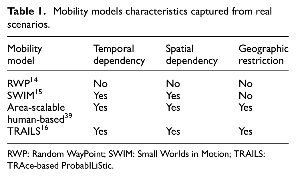
TRAILS is a mobility model in which a user travels to popular places extracted from real scenarios using real paths, as explained in section 3.1. In addition, a user selects a popular place or POI as its destination based on the POI’s popularity, as described in section 3.2. In TRAILS, a graph generator creates a mobility graph with points of interest (POIs) and paths extracted from traces and a simulator imports the graph to controls the users. Figure 1 portrays a didactic representation of a trace-set and its corresponding TRAILS graph.¹⁶

Figure 1.

Comparison between a trace-set and a TRAILS graph.

The paper entitled “TRAILS-A Trace-Based Probabilistic Mobility Model” does not take into account that humans have different routines at distinct moments of the day and that POIs are not equally crowded. This research takes into account both facts by introducing popularity indicators in POIs. A popularity indicator is a time-dependent property that represents the popularity of a POI at different time slots. Section 3.1.1 defines how popularity indicators are estimated, and in section 3.2, we describe how TRAILS uses those indicators in a simulator.¹⁶

In this section, we describe the components of a TRAILS graph. Next, we specify the process used to build graphs from real traces. Finally, we explain the users’ behavior in a TRAILS simulation.

3.1. TRAILS graph

The TRAILS graph is composed by a list of POIs and a list of links. We define a POI as a place where one or more users spend a significant amount of time, for example, a supermarket, an office, or a house. In addition, we define a link as a path connecting two POIs. In TRAILS, paths are extracted from real traces.¹⁶

In a TRAILS graph, a link is a list of coordinates with timestamps between a pair of POIs. In addition, a POI is described with a geographical position, a list of stay times, and a list of popularity indicators. Each stay time represents the amount of time a user can stay in the POI, and each popularity indicator is an element that indicates how congested a POI is at a specific time slot.

This section describes the algorithms used to extract POIs and links from a real scenario.

3.1.1. Extraction of POIs

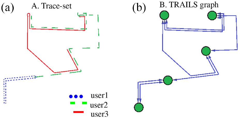
In a real scenario, if a user spends a period longer than a time threshold T in an area limited by a diameter smaller than a constant D. Then, that area represents a POI.

To find a POI, we search for a trace segment that has a duration longer than T and that we can enclose in a circle with a diameter equal to D. To calculate the smallest enclosing circle around a trace segment, we used the “Smallest enclosing circle” algorithm proposed by Emo Welzl and implemented by Project Nayuki.^40,41 Once we find a POI, we search inside the POI additional trace segments that have a duration longer than T. Then, we save the duration of all the trace segments as the POI’s list of stay times. Finally, we build the POI’s list of popularity indicators. Figure 2 shows a graphical illustration of a POI.

Figure 2.

Representation of a POI formed with two trace segments.

In TRAILS, a popularity indicator is equal to the number of users from real traces inside a POI. In a real scenario, the number of users in a POI changes over time. That is why, a POI requires a list of popularity indicators to represent its congestion at different time slots. In addition, we define a time slot as the interval in which the number of users in the POI does not change. TRAILS simulations use the popularity indicators to estimate the probability of a user traveling to a POI.

In a TRAILS simulation, popularity indicators make POIs more or less appealing to users depending on the time slot. Therefore, a simulated user can mimic the routines of users in a real scenario. In addition, the time slots of POIs’ popularity indicators can reduce errors caused by sporadic crowdedness over areas that do not represent an actual place of interest. For example, in a TRAILS simulation, a traffic jam in a roundabout would behave as a POI only during rush hours.

3.1.2. Extraction of links

After we identify the POIs, we extract the links by identifying trace segments connecting a pair of POIs. Once we identify all links, we remove links that we consider unrealistic, and we add new links to guaranty that the TRAILS graph is strongly connected.

We consider a link unrealistic when the link has two consecutive coordinates at a distance longer than a threshold Maximum link gap. For example, if a taxi stops recording its GNSS position for a considerable time while moving around a lake. Then, the taxi’s recorded trace may lead to the false conclusion that it moved through the middle of the lake. Therefore, TRAILS identifies and removes these links from the mobility graph.

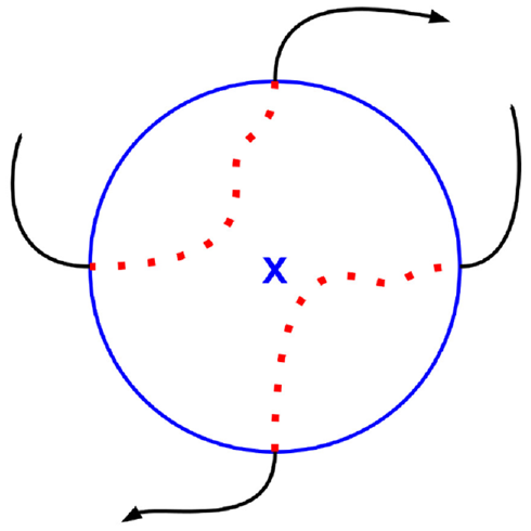
As shown in Figure 3, we search for any pair of POIs connected with links only in one direction. Then, we duplicate those links, and finally, we invert the orientation of the duplicated links. In consequence, if the simulation time is long enough, a user should reach any POI from any other POI.

Figure 3.

Example of the generation of links for a TRAILS graph.

If we do not add the duplicated links in the TRAILS graph, users that arrive to certain POIs would not be able to travel back to POIs they visited before. In other words, the constraints of the users’ mobility would increase over time. Therefore, to guaranty that TRAILS can scale in time, we need to have a strongly connected graph.

3.2. Simulation algorithm

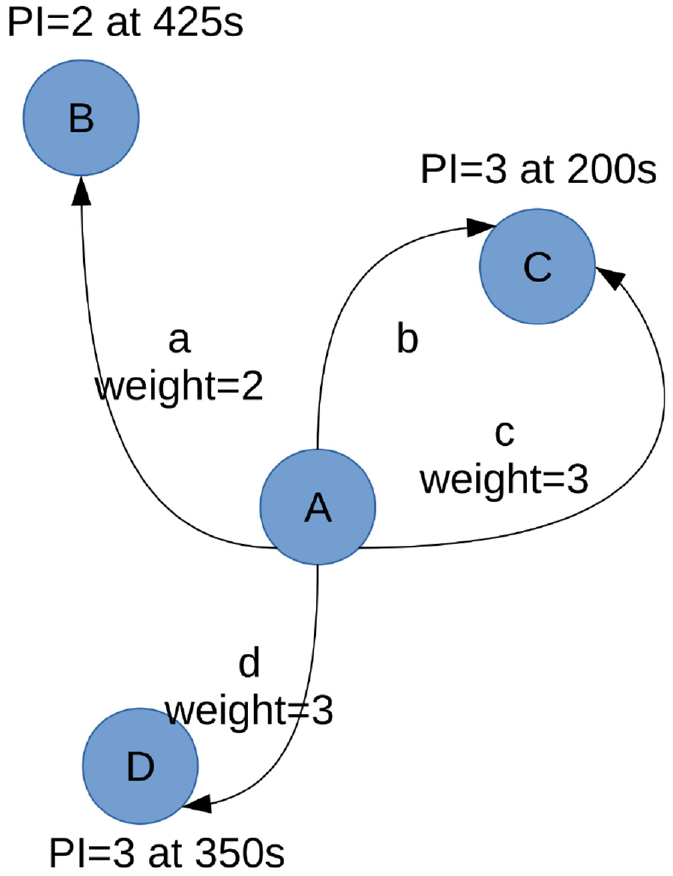
In Figure 4, we present a diagram describing the TRAILS simulation algorithm. The algorithm requires a mobility graph with POIs and links as input parameters, as explained in section 3.1. At the beginning of the simulation, each user starts at a random POI. Then, the user chooses a stay time randomly from the POI’s list. After the stay time is over, the user chooses a random link for each possible destination. Then, the user assigns a weight to each destination POI. The weight is equal to the POI’s popularity indicator estimated at the expected arrival time (AT). After estimating the popularity indicators, the user selects a POI based on a weighted random method. Finally, the user travels to the chosen POI.

Figure 4.

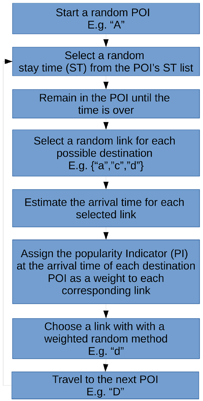
Flowchart of TRAILS algorithm.

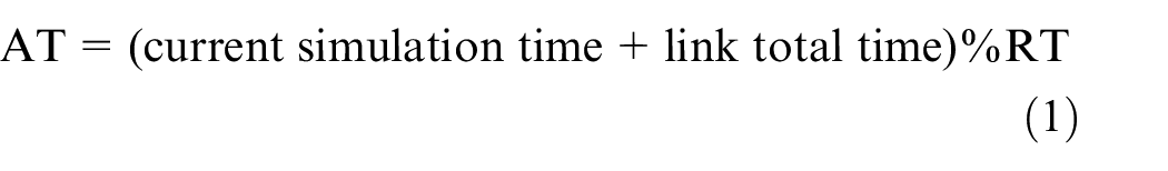
As described in Equation (1), when TRAILS estimates the expected AT, it calculates the residue of the AT extracted from traces modulus the total recorded time (RT) of the real scenario. TRAILS simulations have several advantages over trace-based models. For example, due to Equation (1), it is possible to simulate TRAILS without a time limit. In addition, all users in a TRAILS simulation follow the same logic described in Figures 4 and 5. Therefore, we can simulate the same TRAILS graph with different amounts of users. Furthermore, the TRAILS model reduces the number of events produced in a discrete simulator because a user does not generate new events while it stays in a POI. Accordingly, TRAILS presents an increase in time performance compared to trace-based models, as shown in section 4.4:

AT = (current simulation time + link total time) % RT

(1)

Figure 5.

User behavior in a TRAILS simulation.

4. Results

TRAILS goal is to mimic human social contacts in a real scenario. Therefore, we compare different mobility metrics of TRAILS, real traces, and another fully flexible mobility model such as SWIM.

We chose SWIM as a reference model in the analysis of TRAILS because of its well-defined algorithm and implementation.³⁸ There are more recent models than SWIM such as “An area-scalable human-based mobility model” by Gharib et al. However, Gharib et al. uses the Dijkstra algorithm to search a path between a two hotspot zones, and the Dijkstra algorithm adds a significant computation time overhead for relatively large scenarios. In addition, Gharib et al.³⁹ do not describe a method to extract hotspot zones from real scenarios.

To avoid biased results, we perform our experiments with three different scenarios. We simulate each scenario with its original traces, a TRAILS graph, and two SWIM models with different parameters chosen empirically to approximate the user’s contacts of SWIM simulations to traces.

For each experiment, we compute the TRAILS graphs with a script implemented in the programming language Python 3.⁴² Then, we simulate each mobility model with the discrete simulator OMNeT++ 5.4²⁸ and the framework INET 4.1.⁴³ In addition, we used the model implementation described in the paper “Implementation of the SWIM mobility model in OMNeT++” to perform SWIM simulations. The SWIM implementation requires configuring a set of parameters manually. To analyze the effect of SWIM parameters in our experiments, we execute two SWIM simulations with different sets of parameters for each scenario.³⁸

To find the best set of SWIM parameters, we perform various simulations. Then, we compare the box-plots of the mobility metrics between each SWIM simulation and the original traces. Finally, we select the sets of parameters of the two simulations that presented the fewest differences compared to traces. As shown in Tables 3 –5.

We used our own TRAILS model implementation stored in a GIT repository.⁴⁴ In addition, we used the tool MobilityModelCheck to extract the user’s contacts of each simulation.⁴⁵

In this section, we analyze the users’ contacts by observing three mobility metrics: contact duration, inter-contact time, and repeated contacts. In addition, we describe the repeatability of TRAILS by comparing the variability of mobility metrics between simulations with different random seeds. Furthermore, we discuss the performance of TRAILS in comparison with traces and SWIM simulations by observing the computation time and memory consumption. Finally, we discuss the performance of an OppNet protocol such as Epidemic with different mobility models by comparing the end-to-end delay and the packet delivery ratio in simulations with TRAILS, SWIM, and traces.²⁴

4.1. Scenarios

To study TRAILS and its performance in comparison to traces and SWIM, we used three scenarios: Orlando, New York, and San Francisco. For each scenario, we compute the TRAILS graphs with position trace-sets and the parameters from Table 2.

Table 2.

Parameters to generate TRAILS graphs.

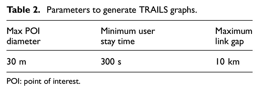
Max POI diameter	Minimum user stay time	Maximum link gap
30 m	300 s	10 km

POI: point of interest.

4.1.1. Orlando

The first scenario, Orlando, represents the movement of 41 pedestrians for 14 h. As shown in Table 3, this section describes the Orlando scenario with its traces, a TRAILS graph, and two sets of SWIM parameters.

Table 3.

Specification of models that represent pedestrians in Orlando.

Simulation parameters	Traces⁴⁶	TRAILS	SWIM1	SWIM2
Number of users	41	41	41	41
Simulation time	51,420 s	51,420 s	51,420 s	51,420 s
Area width	15,422 m	15,422 ms	15,422 m	15,422 m
Area length	17,934.2 m	17,934.2 m	17,934.2 m	17,934.2 m
User speed	*₁	*₁	5 m/s	1 m/s
User wait time	*₂	*₁	U(300 s,1800 s)*₃	U(300 s,1800 s)*₃
Locations/POIs	*₂	896*₁	300	300
Alpha	*₂	*₂	0.5	0.5

TRAILS: TRAce-based ProbabILiStic; SWIM: Small Worlds in Motion; POIs: points of interest.

*₁Parameter extracted from original traces.

*₂Parameter does not apply to the model.

*₃U(A,B) Random value with uniform distribution between A and B.

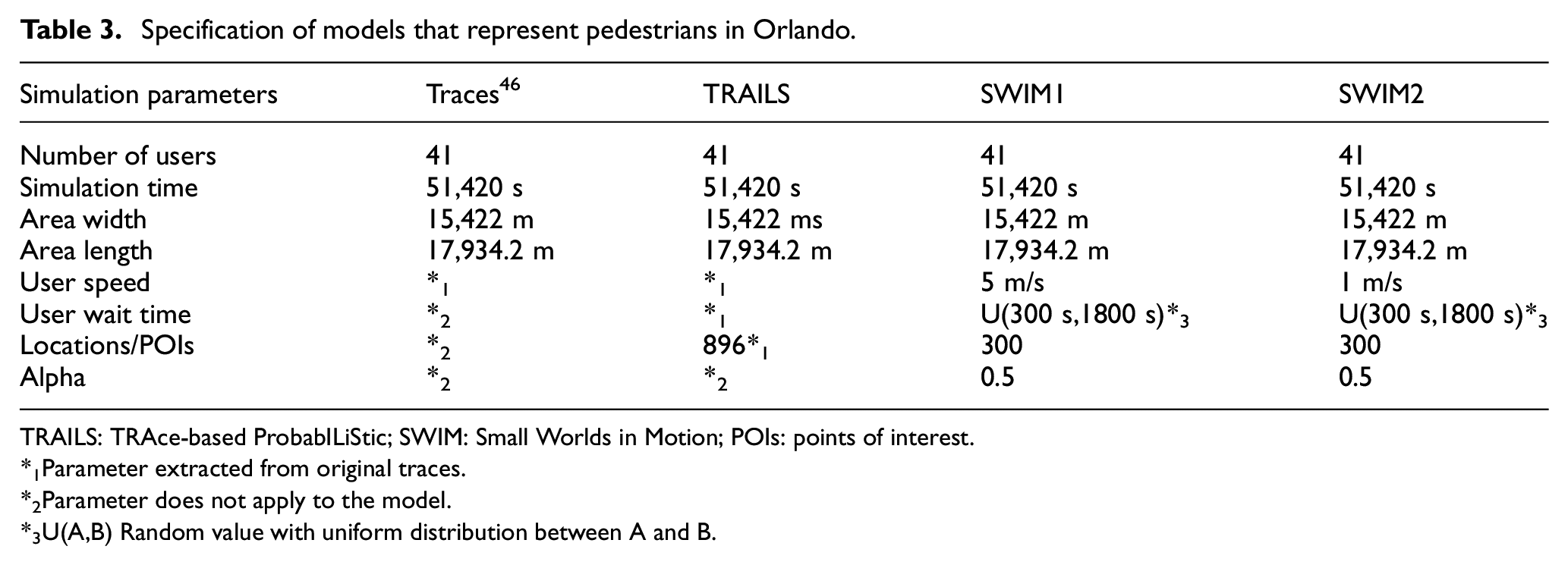
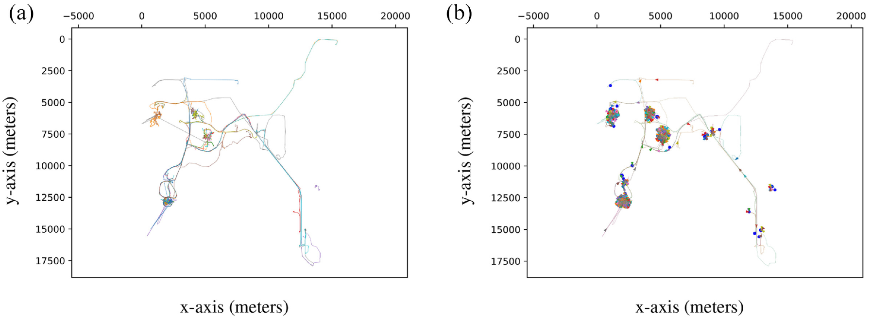
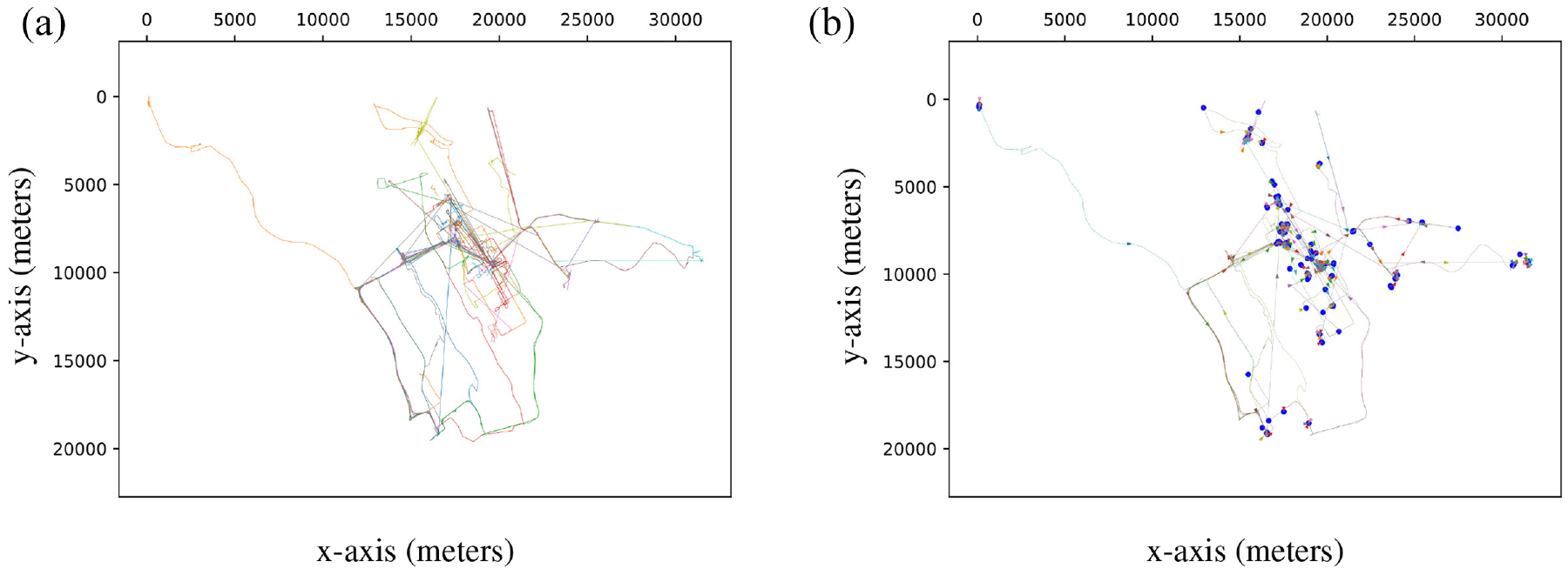
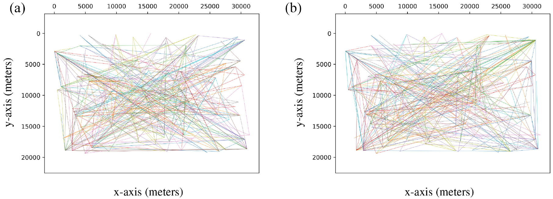
The traces of the Orlando scenario portrayed in Figure 6 are available in the Crawdad database.⁴⁶ The TRAILS graph presented in Figure 6 (right) has 896 POIs and 1433 links. The SWIM simulations described in Figure 7 have the same parameters except for the user speed, as shown in Table 3.

Figure 6.

Traces and TRAILS graph of the Orlando scenario.

Figure 7.

Coordinates of users in SWIM simulations of the Orlando scenario.

4.1.2. New York

The second scenario, summarized in Table 4, represents the movement of 39 pedestrians for 22 h in the city of New York.⁴⁶ Figure 8 (left) presents the GNSS trace-sets. The TRAILS graph shown in Figure 8 (right) describes 195 POIs and 293 links between them. Table 4 shows that the SWIM simulations described in Figure 9 share the same parameters except for the $alpha$ index.

Table 4.

Specification of models that represent pedestrians in New York.

Simulation parameters	Traces⁴⁶	TRAILS	SWIM1	SWIM2
Number of users	39	39	39	39
Simulation time	81,570 s	81,570 s	81,570 s	81,570 s
Area width	31,568.2 m	31,568.2 m	31,568.2 m	31,568.2 m
Area length	19,598.8 m	19,598.8 m	19,598.8 m	19,598.8 m
User speed	*₁	*₁	2 m/s	2 m/s
User wait time	*₂	*₁	U(180 s,3000 s)*₃	U(180 s,3000 s)*₃
Locations/POIs	*₂	195*₁	100	100
Alpha	*₂	*₂	0.5	0.3

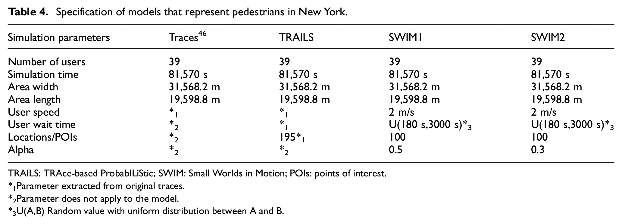
TRAILS: TRAce-based ProbabILiStic; SWIM: Small Worlds in Motion; POIs: points of interest.

*₁Parameter extracted from original traces.

*₂Parameter does not apply to the model.

*₃U(A,B) Random value with uniform distribution between A and B.

Figure 8.

Traces and TRAILS graph of the New York scenario.

Figure 9.

Coordinates of users in SWIM simulations of the New York scenario.

4.1.3. San Francisco

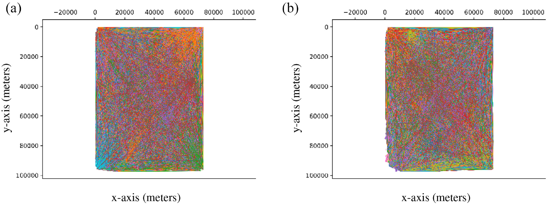
The third scenario portrays in Figure 10 (left) the traces of 536 taxis for 24 days in San Francisco.⁴⁷ As shown in Table 5, the parameters used for the SWIM simulations presented in Figure 11 are the same except for the number of locations. The TRAILS graph shown in Figure 10 (right) describes 40,701 POIs and 189,765 links. In addition, we observe in Figure 10 (right) that TRAILS filters discontinuous traces, as explained in section 3.1.2.

Figure 10.

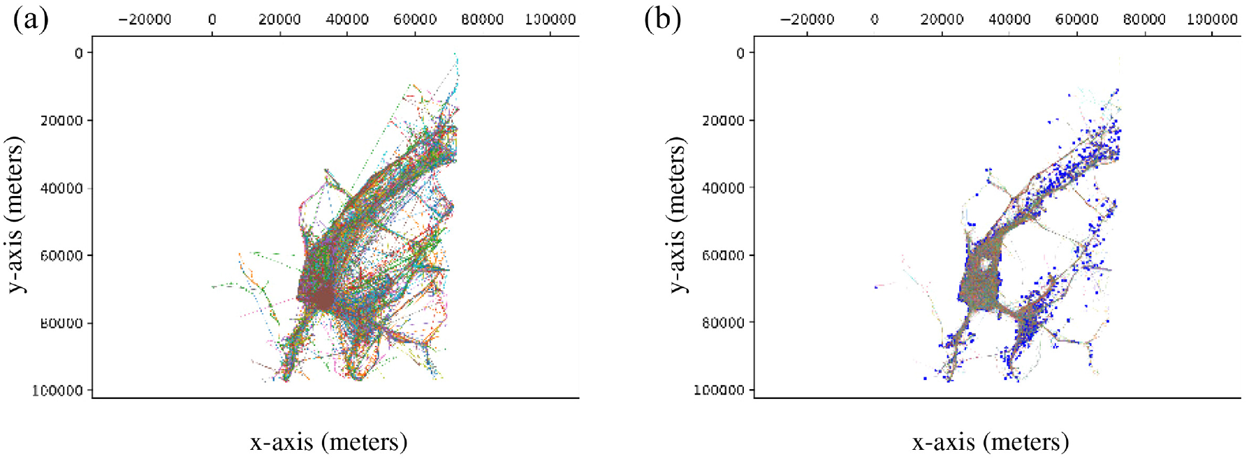
Traces and TRAILS graph of the San Francisco scenario.

Table 5.

Specification of models that represent taxis in San Francisco.

Simulation parameters	Traces⁴⁷	TRAILS	SWIM1	SWIM2
Number of users	536	536	536	536
Simulation time	2,071,530 s	2,071,530 s	2,071,530 s	2,071,530 s
Area width	73,252.7 m	73,252.7 ms	73,252.7 m	73,252.7 m
Area length	97,545.7 m	97,545.7 m	97,545.7 m	97,545.7 m
User speed	*₁	*₁	10 m/s	10 m/s
User wait time	*₂	*₁	U(180 s,3000 s)*₃	U(180 s,3000 s)*₃
Locations/POIs	*₂	40,701*₁	1000	500
Alpha	*₂	*₂	0.5	0.5

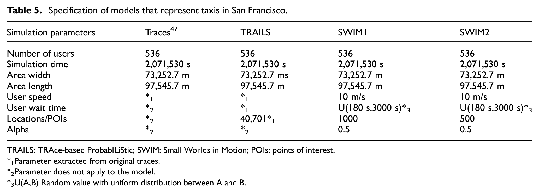
TRAILS: TRAce-based ProbabILiStic; SWIM: Small Worlds in Motion; POIs: points of interest.

*₁Parameter extracted from original traces.

*₂Parameter does not apply to the model.

*₃U(A,B) Random value with uniform distribution between A and B.

Figure 11.

Coordinates of users in SWIM simulations of the San Francisco scenario.

4.1.4. Visual inspection

We observe in Figures 7, 9, and 11 that in the three scenarios, users in SWIM simulations move differently than users in traces. However, Figures 6, 8, and 10 reveal that users in TRAILS follow the same paths described by traces. That is because TRAILS mimics the geographic restrictions of real scenarios, as explained in sections 3.1 and 3.2.

4.2. Analysis of user’s contacts

SWIM requires a manual adaptation of simulation parameters, as shown in Tables 3 –5. However, TRAILS extracts features such as POIs and links directly from the traces, as explained in section 3.1. In this section, we present the difficulties of finding the right set of parameters to approximate the mobility metrics such as contact duration, inter-contact time, and repeated contacts of SWIM and real scenarios. We also describe how TRAILS overcomes those difficulties. In addition, we summarize our findings by comparing the cumulative distribution function (CDF) of the mobility metrics of simulations with SWIM, TRAILS, and traces.

In this research, we define contact duration as the period of two users in contact, inter-contact time as the time between two successive contacts of the same pair of users, and repeated contacts as the number of times the same users were in contact during a simulation.^48,49 In this section, we consider that two users are in contact when they are at a distance shorter than 30 m. Other researchers used the same metrics to describe users’ contacts. For example, the paper “Age Matters: Efficient Route Discovery in Mobile AdHoc Networks Using Encounter Ages” uses the inter-contact time to define users’ link strength.⁵⁰ In addition, the paper “BUBBLE Rap: Social-based forwarding in delay-tolerant networks” uses the contact duration and contact frequency (repeated contacts over time) to measure users’ connectivity.⁵¹

We present each mobility metric with different statistical parameters, such as the median and interquartile range (IQR). We use the median because it is a better indicator of the probability density function (PDF) center than the arithmetic mean when the distribution of the metric is asymmetric.⁵² In addition, we use the IQR to describe the dispersion of the data around the median.⁵³ We also represent the metrics graphically with box-plots and the CDF. Box-plots depict the mobility metrics with their median and their quartiles,⁵⁴ while the CDF portrays the metrics’ distribution.⁵⁵

4.2.1. Contact duration and inter-contact time

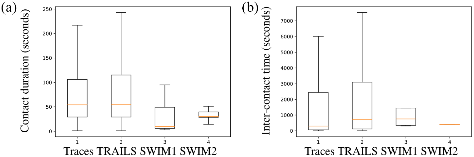
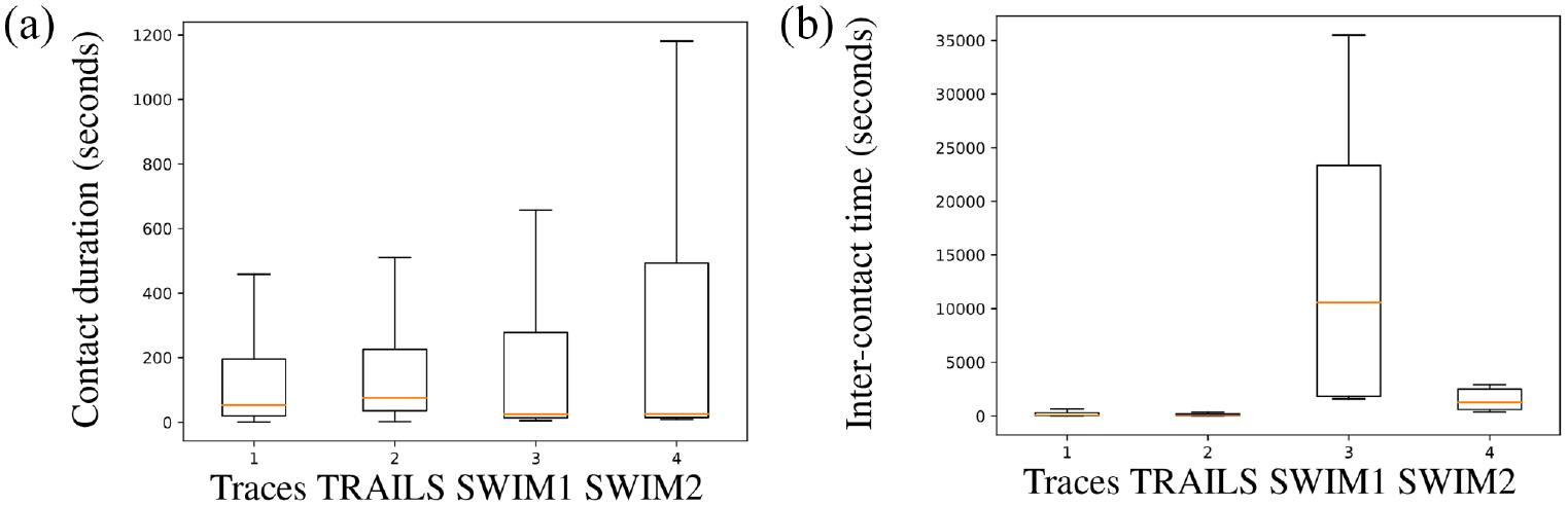
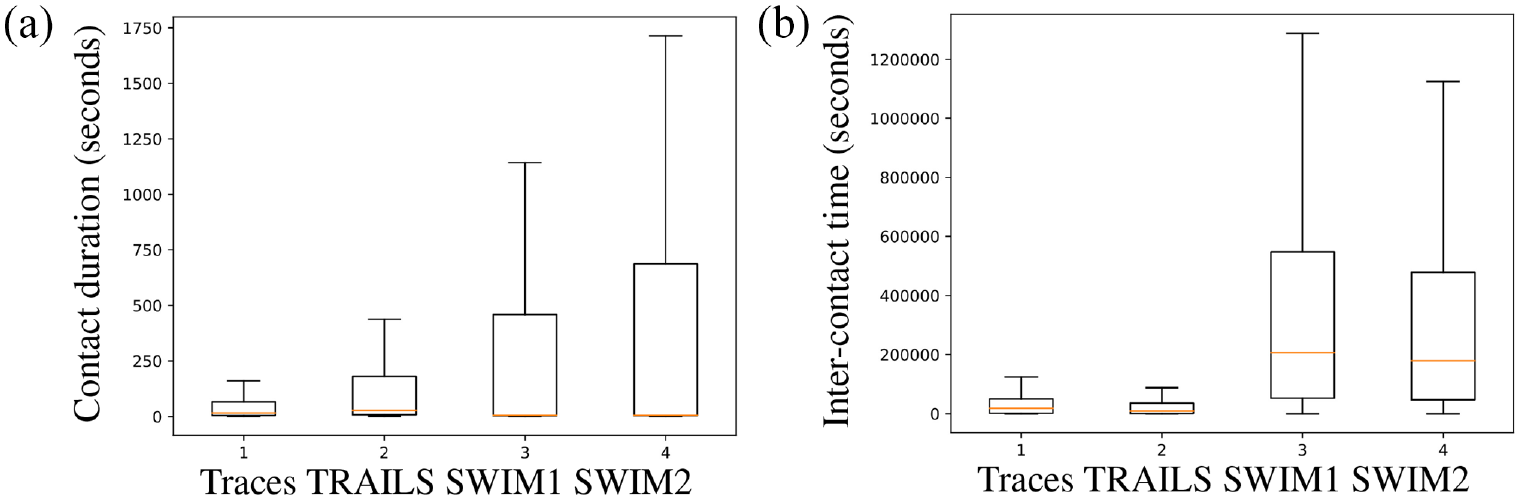
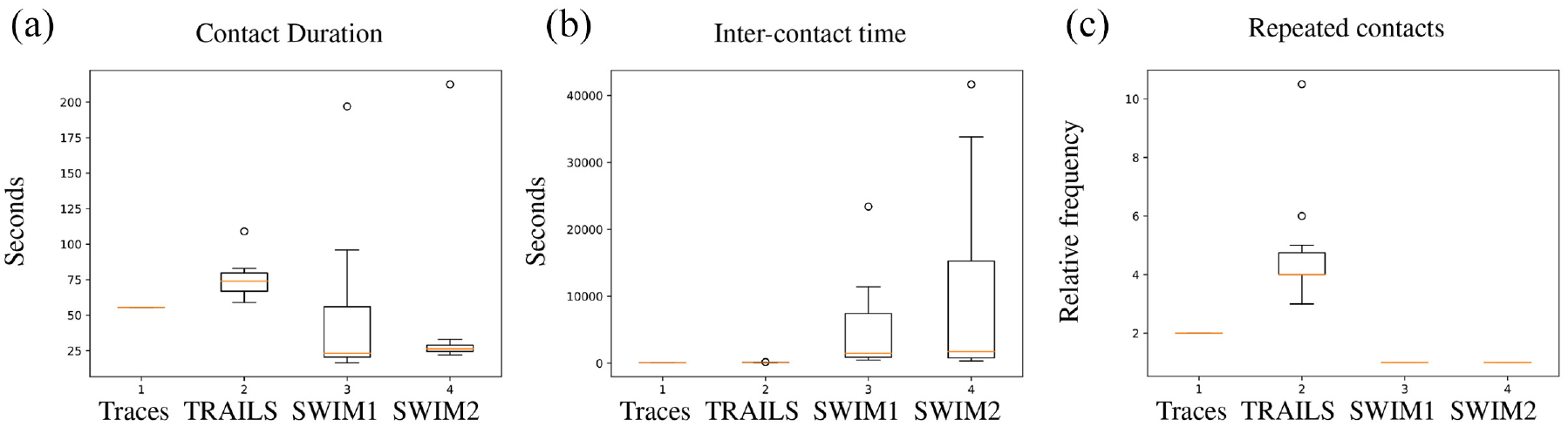
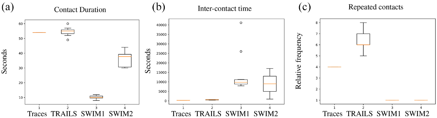
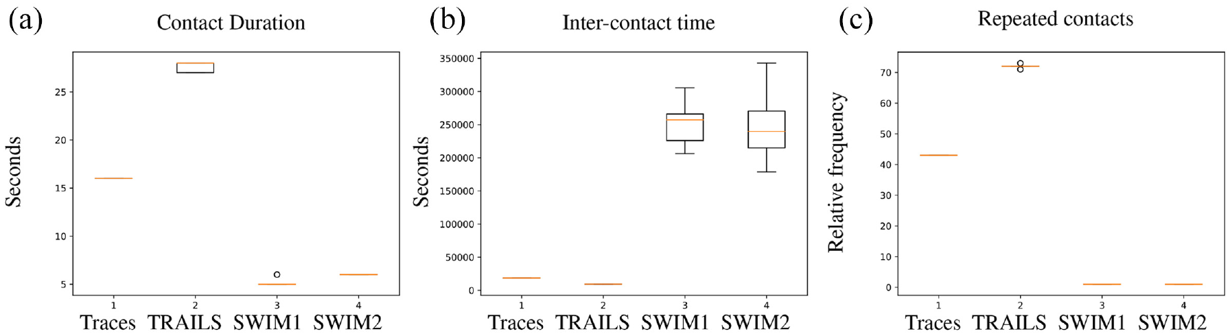
In Figures 12 –14, we use box-plots to portray the contact duration and inter-contact time of user’s contacts of the three scenarios. Each figure shows the results of real traces, a TRAILS simulation, and two SWIM simulations. We describe the simulation parameters for each scenario in section 4.1.

Figure 12.

Box-plots of simulations of the Orlando scenario.

Figure 13.

Box-plots of simulations of the New York scenario.

Figure 14.

Box-plots of simulations of the San Francisco scenario.

In Figure 12, we observe that in the Orlando scenario, the median of contact duration of the original trace-set is more similar to the second SWIM simulation (SWIM2) than to the first SWIM simulation (SWIM1). However, the contact duration IQR of the same trace-set is more similar to SWIM1 than to SWIM2. In addition, in Figures 13 and 14, we see that for the New York and San Francisco scenarios, the contact duration IQR of traces is closer to SWIM1 than that is to SWIM2. Meanwhile, the inter-contact time IQR of New York’s and San Francisco’s traces is closer to SWIM2 than that is to SWIM1. In conclusion, if we want to approximate the properties of users’ contacts of SWIM simulations to real traces, we may need to spend considerable effort performing several SWIM simulations until we find an adequate set of SWIM parameters.

Figures 12 –14 also reveal that contrary to SWIM, the medians and IQR of contact duration and inter-contact time are similar between TRAILS simulations and traces in the three scenarios. For example, in Figure 13, the mean absolute percentage error (MAPE) of the median contact duration between TRAILS and traces is 0.4, and the MAPE of the median contact duration between SWIM1 and traces is 0.53. However, the MAPE of the median inter-contact time between TRAILS and traces is 0.32, and the MAPE of the median inter-contact time between SWIM1 and traces is 125. In conclusion, we do not need to spend several iterations trying out different parameters to improve the results of TRAILS simulations.

4.2.2. Repeated contacts

As shown in Figure 15, for the three scenarios, the number of repeated contacts of SWIM simulations is considerably lower than the number of repeated contacts of traces. However, the box-plots of repeated contacts of TRAILS are more approximate to traces than SWIM simulations. The reason behind it is that a user in SWIM has a lower probability of making contact with other users because it can move to any position in a square area, as revealed in Figures 7, 9, and 11. However, Figures 6, 8, and 10 show that a user in a real scenario has more geographical restrictions such as buildings or lakes. In addition, TRAILS replicates those geographical restrictions by allowing a user to move only through predefined links extracted from traces. Therefore, in TRAILS simulations as in real scenarios, users have a higher probability to get in contact with each other.

Figure 15.

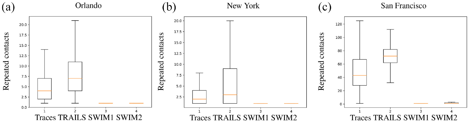
Box-plots of simulations of repeated contacts.

4.2.3. CDF of contact’s metrics

We observe in Figures 16 and 17 that the CDF of TRAILS and traces is smooth compared to SWIM simulations. The underlying reason is that the smoothness of the CDF depends on the number of contacts between users. As explained in section 4.2.2, SWIM simulations reproduced a relatively low number of contacts. Furthermore, we observe in Figures 16 –18 that without the need for parameter tuning, TRAILS’ CDFs present a lower difference between real traces than SWIM simulations.

Figure 16.

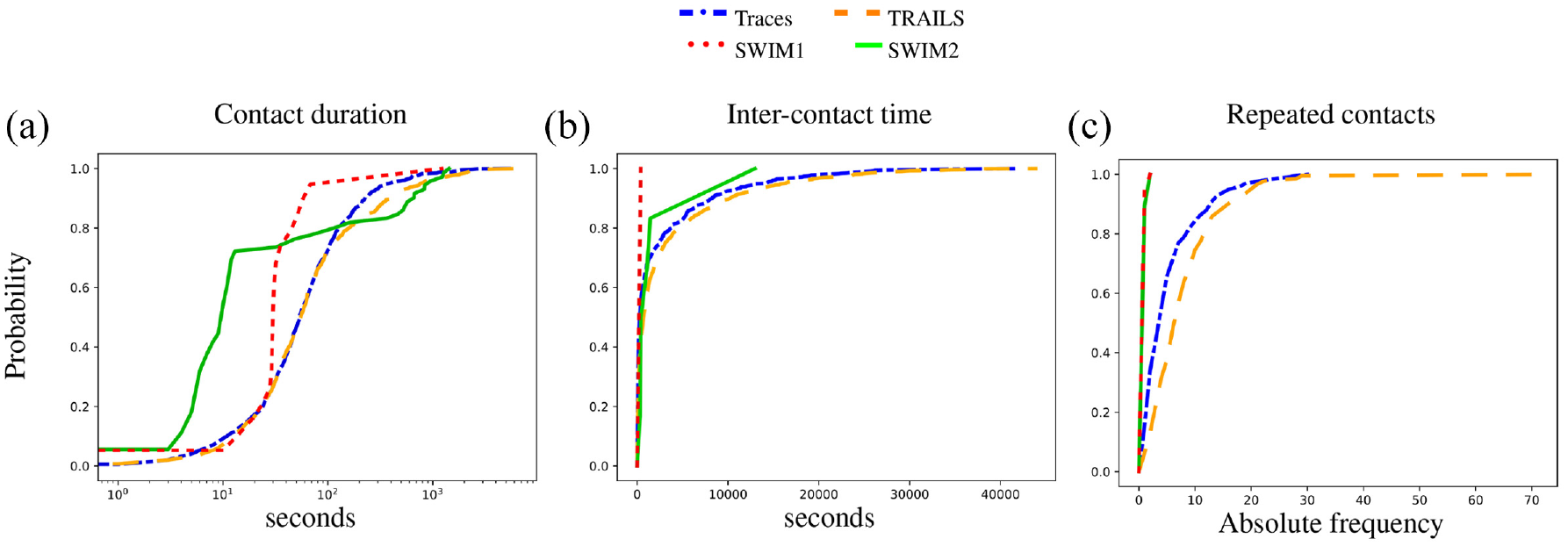
CDF of the Orlando scenario.

Figure 17.

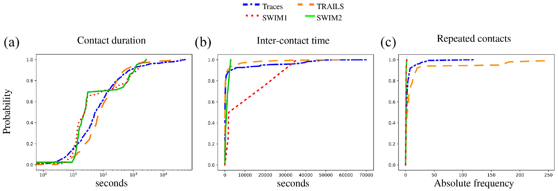
CDF of the New York scenario.

Figure 18.

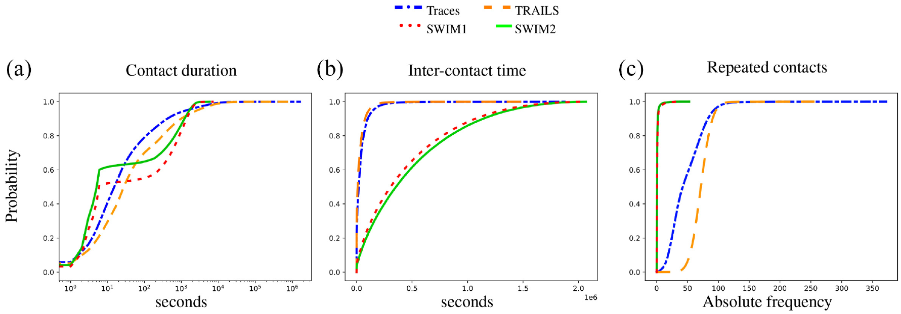
CDF of the San Francisco scenario.

4.3. Results’ variability between simulations

If two simulations of the same scenario are very different, each simulation will lead to a different conclusion. That is why, it is vital to use a mobility model where the variability in the results between simulations is not high. In this section, we analyze the reliability of the TRAILS model compared to SWIM by performing several simulations with the same scenario and then observing the medians of mobility metrics of each simulation.

In Figures 19 –21, we describe the spread of medians of mobility metrics of TRAILS simulations, SWIM simulations, and the real traces of the scenarios described in section 4.1. To avoid misleading results caused by outliers, for each scenario, we computed five TRAILS simulations and five SWIM simulations for each set of parameters (SWIM1 and SWIM2).

Figure 19.

Box-plots of medians of mobility metrics of the simulations of the New York scenario.

Figure 20.

Box-plots of medians of mobility metrics of the simulations of the Orlando scenario.

Figure 21.

Box-plots of medians of mobility metrics of the simulations of the San Francisco scenario.

In each scenario portrayed in Figures 19 –21, we observe that the medians of inter-contact time of TRAILS simulations present a lower dispersion than SWIM. In the case of the contact duration, the spread of the medians of TRAILS and SWIM is similar. However, the medians of the contact duration of TRAILS simulations are more similar to traces than the SWIM simulations. In case of repeated contacts, the medians of SWIM simulations are always around one contact per simulation. The low number of repeated contacts for SWIM simulations is related to their low contact probability, as explained in section 4.2.2.

In conclusion, the repeatability of results in TRAILS simulations is higher than SWIM, especially for the inter-contact time. The reason behind it is that in TRAILS, a node can travel only to a POI that has a direct link with the user’s current POI. However, a user in SWIM can travel from a given location to any other location. Consequently, the probability that a node would choose the same destination is higher in TRAILS simulations than it is in SWIM.

4.4. Performance analysis of TRAILS

This section describes the computation time of TRAILS, traces, and SWIM. Then, it discusses the disk memory used by real traces versus TRAILS graphs. After, this section discusses the memory required (log memory) to record simulation results for each model. Finally, it presents how the computation time and log memory are affected when TRAILS simulations are scaled by simulation time and by the number of users.

In order to present a performance analysis, we performed the TRAILS graph generation and the model simulation in a computer with a processor Intel i7 2.60 GHz and a memory RAM of 16 GB under a 64-bit Linux operating system.

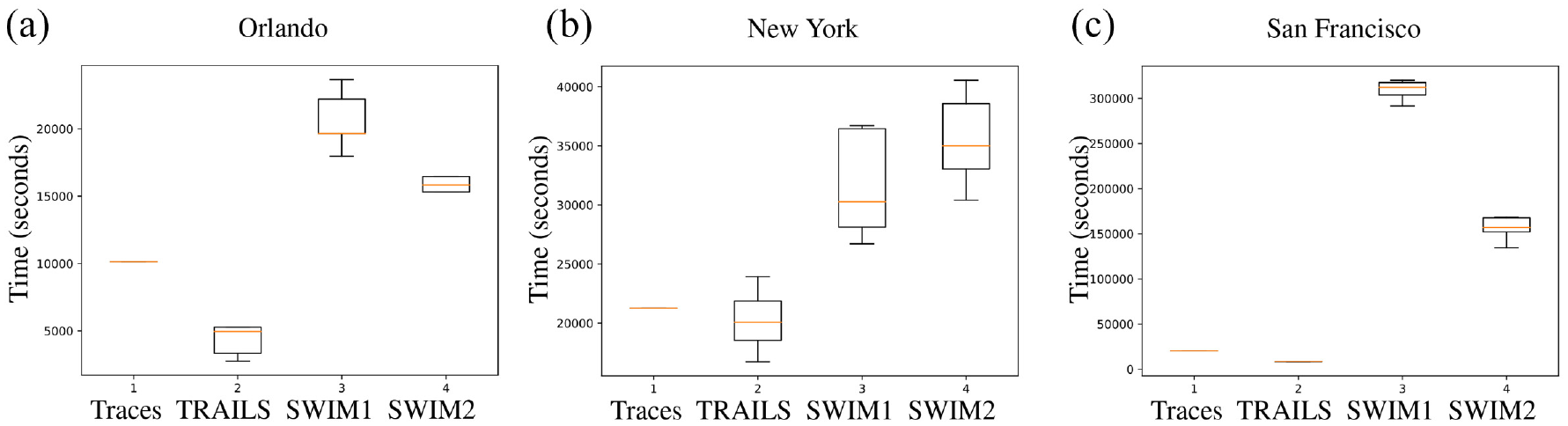
As we observe in Tables 6 and 7, the computation time and memory usage of the San Francisco scenario is considerably higher than the scenarios Orlando and New York. The reason is mostly the difference in the number of users, San Francisco has more than 500 users while Orlando and New York have less than 50 users. In section 4.4.3, and Figure 23, we show that the computation time and memory consumption have a logarithmic relation to the number of users.

Table 6.

Computation time of different models of each mobility scenario.

Model	Orlando	New York	San Francisco
Traces *₂	4.6623 s	6.739 s	24,374.6 s
TRAILS *₁	1.5628 s	1.152 s	200.42 s
TRAILS *₃	4.274 s	6.405 s	18,370.16 s
SWIM *₃	4.662 s	6.286 s	11,569.58 s

TRAILS: TRAce-based ProbabILiStic; SWIM: Small Worlds in Motion.

*₁Computation time of TRAILS graph generation.

*₂Computation time of a model simulation.

*₃Mean of the computation time of five simulations.

Table 7.

Memory size of mobility graphs.

Model	Orlando	New York	San Francisco
Traces	3.6 MB	3.2 MB	379 MB
TRAILS	319.5 KB	124.5 KB	154.4 MB

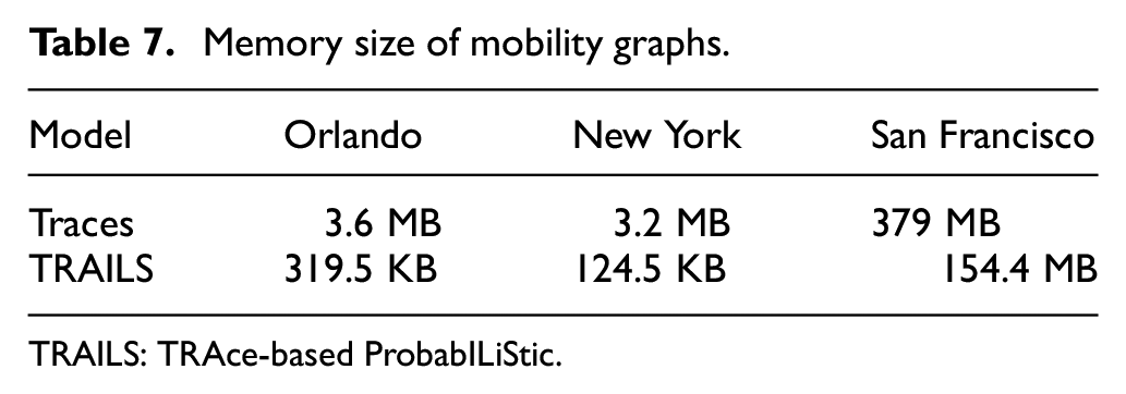
TRAILS: TRAce-based ProbabILiStic.

4.4.1. Computation time

As described in Table 6, TRAILS simulations require less computation time than real traces because TRAILS reduces the number of events in a discrete simulator, as explained in section 3.2. However, SWIM simulations require less computation time than TRAILS. However, we may require several SWIM simulations to adapt SWIM parameters to a specific scenario, as demonstrated in section 4.2. In addition, the generation of TRAILS graphs requires an additional computation time. Still, for large scenarios such as San Francisco, this time is significantly lower than the time difference between the computation time of TRAILS simulations and traces.

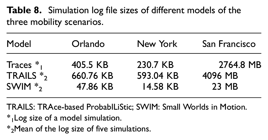
4.4.2. Memory performance

According to graph sizes described in Table 7, TRAILS graphs require less memory than traces. The reason behind it is that TRAILS transforms several user coordinates into a single POI, as explained in section 3.1.

Table 8 shows that the log files generated by SWIM simulations are shorter than log files generated by traces. However, the log files generated by TRAILS simulations are larger than traces’ log files. According to the implementation of the algorithm to record simulation data,⁴⁵ the size of the log file is related with the total number of contacts. In addition, we can see in Figures 19 –21 that the number of repeated contacts in SWIM is lower than it is in TRAILS.

Table 8.

Simulation log file sizes of different models of the three mobility scenarios.

Model	Orlando	New York	San Francisco
Traces *₁	405.5 KB	230.7 KB	2764.8 MB
TRAILS *₂	660.76 KB	593.04 KB	4096 MB
SWIM *₂	47.86 KB	14.58 KB	23 MB

TRAILS: TRAce-based ProbabILiStic; SWIM: Small Worlds in Motion.

*₁Log size of a model simulation.

*₂Mean of the log size of five simulations.

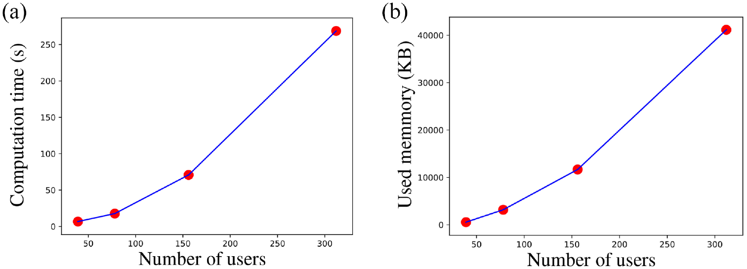
4.4.3. Scalability effect in TRAILS performance

As explained in section 3.2, with TRAILS, we can simulate a scenario with a higher number of users or a longer simulation time than the original traces. For example, the trace-set of the New York scenario has 39 users and an RT of 81,570 s. However, in Figure 23, we show the performance of TRAILS simulations with a simulation time of 81,570 s and up to 312 users. Figure 22 describes the performance of TRAILS simulations with 39 users and with simulation time up to 652,560 s.

Figure 22.

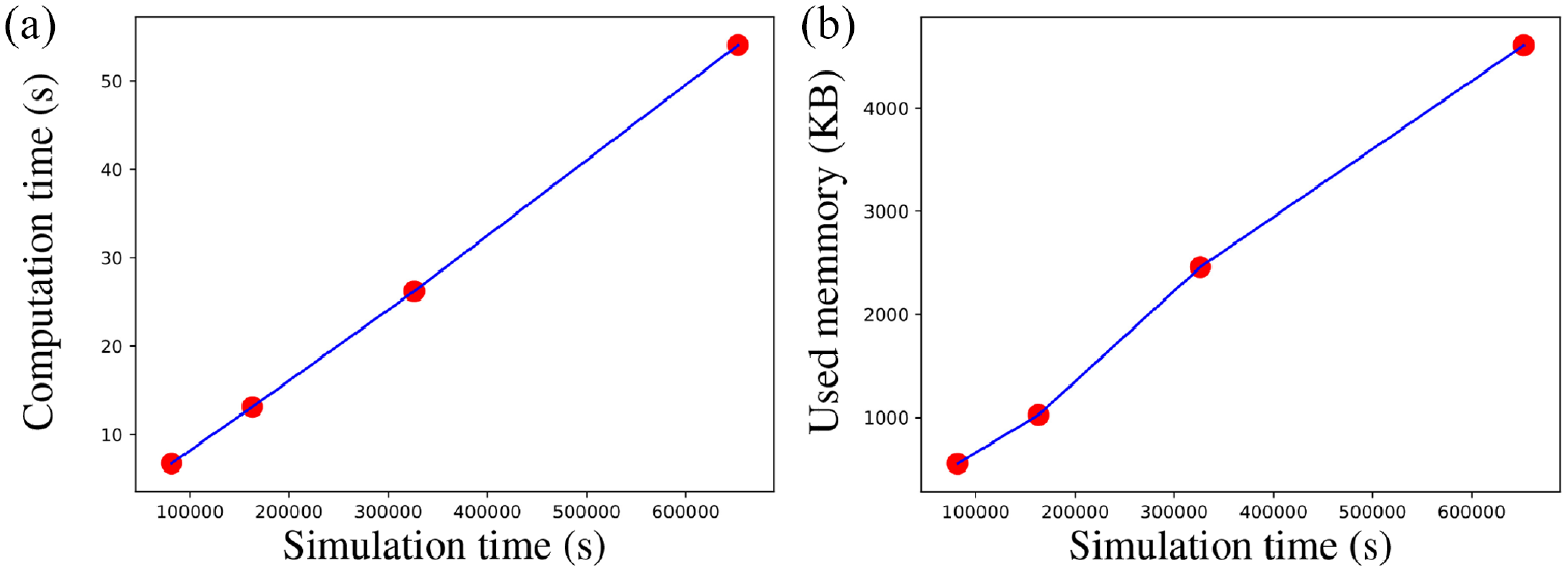
Mean of the performance metrics of the TRAILS model of the New York scenario scaled by simulation time.

Figure 22 portrays that the computation time and the log memory size have a positive linear relationship with the simulation time; however, in Figure 23, the computation time and the log memory size have a positive logarithmic relationship with the number of users. Those results respond to the hypothesis that if a scenario does not change drastically, an increase in time should produce a linear increase in users’ contacts. However, an increase in the number of users should produce an exponential increase in users’ contacts. In addition, sections 4.4.1 and 4.4.2 reveal a strong relationship between performance and the number of users’ contacts.

Figure 23.

Mean of the performance metrics of the TRAILS model of the New York scenario scaled by number of users.

4.5. Network communication

One of the reasons to use mobility models is to measure the performance of OppNet protocols. However, the same protocol produces different results with different mobility models. For this purpose, we describe how communication metrics vary depending on the mobility model.

In this section, we repeat the simulations described in section 4.3, but now each user forwards data using an OppNet protocol. In our simulations, each user generates a broadcast message of 10 KB each 900 s. Later, each message is propagated using the Epidemic protocol.²⁴ To simulate the Epidemic protocol with TRAILS, traces, and SWIM, we used the OPS framework alongside the discrete simulator OMNeT++.²⁷

In Figure 24, we present the delivery ratio, and in Figure 25, we describe the mean end-to-end delay of each simulation.²²

Figure 24.

Box-plots of the delivery ratio of the simulations of the New York scenario.

Figure 25.

Box-plots of the end-to-end delay of the simulations of the New York scenario.

Figures 24 and 25 reveal that the medians of the end-to-end delay and the delivery ratio of TRAILS simulations are more similar to traces than SWIM simulations. In addition, we observe in Figure 24 that the median of the delivery ratio of TRAILS simulations is always higher than traces. Similarly, Figure 25 shows that the median of the mean end-to-end delay of TRAILS simulations is always lower than traces. The reason behind these results is that any user in a TRAILS simulation can visit any POI, as explained in section 3.1.2. However, a user in a real scenario may never visit all POIs. Consequently, in TRAILS, a user can get in contact with any other user, while in real traces, there are users that may never get in contact.

5. Conclusion

The TRAILS mobility model can capture specific mobility characteristics of realistic scenarios such as temporal dependency, spatial dependency, and geographic restrictions. A user mimics a real scenario’s temporal dependency in a TRAILS simulation by moving between POIs with the same speed as a user in traces. As shown in section 3.1.1, TRAILS reflects the spatial dependency of traces by capturing the relation between users and POIs with popularity indicators. A user in a TRAILS simulation only moves through links between POIs. In addition, links describe real paths of traces. Therefore, TRAILS represents the geographic restrictions of real scenarios.

The movement patterns of users in real scenarios vary over time because they have different routines at different hours or days. Therefore, the interaction between users also changes. TRAILS considers these changes by matching the probability of traveling to a POI with the number of users the POI had in the original traces, as described in section 3.2.

It is possible to simulate the same TRAILS graph with a different number of users and simulation time. Therefore, unlike trace-based models, TRAILS is a fully scalable and flexible mobility model, as explained in section 3.2.

TRAILS graphs are capable of summarizing several trace-coordinates in a single POI. In consequence, the data size of TRAILS graphs is smaller than traces. In addition, a TRAILS simulation produces fewer events than a simulation of traces because when a user stays in a POI, it does not generate additional events. However, in a simulation of traces, a user may produce events even if the user is not moving or it is moving inside a small area. Therefore, TRAILS simulations require less computation time than traces, as shown in section 4.4.

Although the implemented TRAILS model presents a satisfactory performance in computation time and memory consumption, we determined that TRAILS cannot mimic real traces perfectly. However, we can scale TRAILS scenarios by simulation time and the number of mobile users in a way that we cannot achieve with trace-based mobility models.

A single user in TRAILS mimics the behavior of all users of real traces, and it does not take into account the differences of the mobility patterns among real users. Therefore, section 4.5 shows that we get a higher delivery ratio and a lower end-to-end delay when we evaluate the performance of the Epidemic Network protocol with TRAILS rather than real traces. As future work, we propose to categorize users into communities, generate a TRAILS graph for each community, and simulate users assigned to different graphs. In our proposed solution, two users who belong to different communities will have different POIs but also common POIs. Therefore, we believe that our future work will capture the spatial dependency of real scenarios in a more effective way.

In summary, the TRAILS mobility model can capture mobility characteristics of realistic scenarios. TRAILS graphs take into consideration the dynamic interaction between users and POIs. In addition, we can scale TRAILS simulations by the number of users and the simulation time. Moreover, TRAILS graphs use less memory than traces, and simulating TRAILS graphs requires less computation time than trace-based models.

Footnotes

Funding

This research received no specific grant from any funding agency in the public, commercial, or not-for-profit sectors.

ORCID iD

Leonardo Sarmiento

Author biographies

Leonardo Sarmiento is a PhD student under Professor Dr Anna Förster in the Sustainable Communication Networks group at the University of Bremen. He is also a teaching assistant at the Universidad Politécnica Salesiana in Ecuador.

Anna Förster is a full Professor at the University of Bremen in Germany and leading the Sustainable Communication Networks group. She is also the director of the Bremen Spatial Cognition Center.

References

Bhoi

Analysis & comparison of mobility models for ad-hoc network. Int J Recent Innov Trend Comput Commun 2014; 2: 1357–1362.

Lee

Hong

Kim

, et al. SLAW: a mobility model for human walks. In: Proceedings of the IEEE INFOCOM 2009, Rio de Janeiro, Brazil, 19–25 April 2009, pp. 855–863. New York: IEEE.

Kuppusamy

Sarmiento

Udugama

, et al. Community-based mobility model and probabilistic ORBIT mobility model implementations in OMNeT++. In: Proceedings of the 5th international OMNeT++ community summit, 2018, pp. 23–34, https://easychair.org/publications/open/H5pq

Tian

Meng

. Comparison survey of mobility models in vehicular ad-hoc network (VANET). In: Proceedings of the 2020 IEEE 3rd international conference on automation, electronics and electrical engineering (AUTEEE), Shenyang, China, 20–22 November 2020, pp. 337–342. New York: IEEE.

Habaebi

Merrad

Islam

, et al. Extending CloudSim to simulate sensor networks. Simulation. Epub ahead of print 20 June 2022. DOI: 10.1177/00375497221105530.

Dong

Dargie

A survey on mobility and mobility-aware MAC protocols in wireless sensor networks. IEEE Commun Surv Tut 2012; 15: 88–100.

Mainwaring

Polastre

Szewczyk

, et al. Wireless sensor networks for habitat monitoring. In: Proceedings of the 1st ACM international workshop on wireless sensor networks and applications, 2002, pp. 88–97, https://people.eecs.berkeley.edu/~culler/papers/wsna02.pdf

Lee

Song

, et al. Wireless sensor network design for tactical military applications: remote large-scale environments. In: Proceedings of the MILCOM 2009—2009 IEEE military communications conference, Boston, MA, 18–21 October 2009, pp. 1–7. New York: IEEE.

Taleb

Alhmiedat

Hassan

OAH

. A survey of sink mobility models for wireless sensor networks. J Emerg Trend Comput Inform Sci 2013; 4: 679–687.

10.

Rhee

Lee

Hong

, et al. Demystifying the levy-walk nature of human walks. Technical Report, North Carolina State University (NCSU), Raleigh, NC, 2008.

11.

Tabassum

Salehi

Hossain

Fundamentals of mobility-aware performance characterization of cellular networks: a tutorial. IEEE Commun Surv Tut 2019; 21: 2288–2308.

12.

Munjal

Camp

Aschenbruck

Changing trends in modeling mobility. J Electr Comput Eng 2012; 2012: 372572.

13.

Rodolakis

Analytical models and performance evaluation in massive mobile ad hoc networks. PhD Thesis, Université Paris, Paris, 2006.

14.

Bettstetter

Hartenstein

Pérez-Costa

Stochastic properties of the random waypoint mobility model. Wirel Netw 2004; 10: 555–567.

15.

Mei

Stefa

SWIM: a simple model to generate small mobile worlds. In: Proceedings of the IEEE INFOCOM 2009, Rio de Janeiro, Brazil, 2 June 2009, pp. 2106–2113. New York: IEEE.

16.

Förster

Bin Muslim

Udugama

TRAILS—a trace-based probabilistic mobility model. In: Proceedings of the 21st ACM international conference on modeling, analysis and simulation of wireless and mobile systems, 2018, pp. 295–302, https://www.researchgate.net/publication/328544518_TRAILS_-_A_Trace-Based_Probabilistic_Mobility_Model

17.

Temene

Sergiou

Georgiou

, et al. A survey on mobility in wireless sensor networks. Ad Hoc Netw 2022; 125: 102726.

18.

Dede

Förster

Hernández-Orallo

, et al. Simulating opportunistic networks: survey and future directions. IEEE Commun Surv Tut 2017; 20: 1547–1573.

19.

Quy

Nam

Linh

, et al. A survey of QoS-aware routing protocols for the MANET-WSN convergence scenarios in IoT networks. Wirel Pers Commun 2021; 120: 49–62.

20.

Huang

Lan

Tsai

. A survey of opportunistic networks. In: Proceedings of the 22nd international conference on advanced information networking and applications—workshops (AINA workshops 2008), Ginowan, Japan, 25–28 March 2008, pp. 1672–1677. New York: IEEE.

21.

Fanian

Rafsanjani

MK.

Cluster-based routing protocols in wireless sensor networks: a survey based on methodology. J Netw Comput Appl 2019; 142: 111–142.

22.

Timcenko

Stojanovic

Rakas

SB.

MANET routing protocols vs. mobility models: performance analysis and comparison. In: Proceedings of the 9th WSEAS international conference on applied informatics and communications, 2009, pp. 271–276, https://www.researchgate.net/publication/229035399_MANET_routing_protocols_vs_mobility_models_performance_analysis_and_comparison

23.

Balasubramanian

Levine

Venkataramani

DTN routing as a resource allocation problem. In: Proceedings of the 2007 conference on applications, technologies, architectures, and protocols for computer communications, 2007, pp. 373–384, https://citeseerx.ist.psu.edu/viewdoc/download?doi=10.1.1.129.9966&rep=rep1&type=pdf#:~:text=The%20inherent%20uncertainty%20about%20network,path%20with%20extremely%20limited%20information.

24.

Vahdat

Becker

Epidemic routing for partially connected ad hoc networks. Technical Report CS-200006, Duke University, Durham, April 2000.

25.

Keränen

Ott

Kärkkäinen

. The ONE simulator for DTN protocol evaluation. In: Proceedings of the 2nd international conference on simulation tools and techniques, 2009, https://www.netlab.tkk.fi/tutkimus/dtn/theone/pub/the_one_simutools.pdf

26.

Papanikos

Akestoridis

Papapetrou

Adyton: a network simulator for opportunistic networks, 2015, https://github.com/npapanik/Adyton

27.

Udugama

Förster

Dede

, et al. Opportunistic networking protocol simulator for OMNeT++, 2017, https://arxiv.org/abs/1709.02210

28.

Varga

OMNeT++ discrete event simulation system, version 5.4, 2019, https://citeseerx.ist.psu.edu/viewdoc/download?doi=10.1.1.122.1688&rep=rep1&type=pdf

29.

Ali

Suleman

Uzmi

. MMAC: a mobility-adaptive, collision-free MAC protocol for wireless sensor networks. In: Proceedings of the PCCC 2005: 24th IEEE international performance, computing, and communications conference, 2005, Phoenix, AZ, 5 July 2005, pp. 401–407. New York: IEEE.

30.

Tuduce

Gross

. A mobility model based on WLAN traces and its validation. In: Proceedings of the IEEE 24th annual joint conference of the IEEE computer and communications societies, Miami, FL, 13–17 March 2005, vol. 1, pp. 664–674. New York: IEEE.

31.

Marin-Perianu

Havinga

, et al. Movement-based group awareness with wireless sensor networks. In: Proceedings of the international conference on pervasive computing, White Plains, NY, 19–23 March 2007, pp. 298–315. Berlin: Springer.

32.

Čapkun

Hamdi

Hubaux

JP.

GPS-free positioning in mobile ad hoc networks. Clust Comput 2002; 5: 157–167.

33.

Burgard

Fox

Hennig

, et al. Estimating the absolute position of a mobile robot using position probability grids. In: Proceedings of the national conference on artificial intelligence, 1996, pp. 896–901, https://citeseerx.ist.psu.edu/viewdoc/download?doi=10.1.1.114.9606&rep=rep1&type=pdf

34.

Kotz

Henderson

Crawdad: a community resource for archiving wireless data at Dartmouth. IEEE Pervas Comput 2005; 4: 12–14.

35.

López

Wikiloc: database and sharing platform for GNSS traces, 2021, https://www.wikiloc.com/

36.

Helmy

Bai

Hsu

Mobilib: community-wide library of mobility and wireless networks measurements, 2008, https://www.cise.ufl.edu/~helmy/MobiLibOld.htm

37.

Bai

Helmy

A survey of mobility models. Wirel Adhoc Netw 2004; 206: 147.

38.

Udugama

Khalilov

Muslim

, et al. Implementation of the SWIM mobility model in OMNeT++, 2016, https://arxiv.org/abs/1609.05199

39.

Gharib

Foroozani

Rezaei

, et al. An area-scalable human-based mobility model. Comput Netw 2020; 177: 107300.

40.

Welzl

Smallest enclosing disks (balls and ellipsoids). Berlin: Springer, 1991, pp. 359–370.

41.

Project Nayuki. Smallest enclosing circle, 2018, https://www.nayuki.io/page/smallest-enclosing-circle

42.

Oliphant

TE.

Python for scientific computing. Comput Sci Eng 2007; 9: 10–20.

43.

Varga

INET framework for the OMNeT++ discrete event simulator, version 4.1, 2019, https://inet.omnetpp.org/

44.

Sarmiento

Förster

TRAILS—OMNeT-implementation: trace based probabilistic, 2021, https://github.com/ComNets-Bremen/TRAILS—OMNeT-Implementation

45.

Udugama

Förster

MobilityModelCheck, 2019, https://github.com/ComNets-Bremen/MobilityModelCheck

46.

Rhee

Shin

Hong

, et al. The ncsu/mobilitymodels dataset (v. 2009-07-23), 2009, https://crawdad.org/ncsu/mobilitymodels/

47.

Piorkowski

Sarafijanovic-Djukic

Grossglauser

The epfl/mobility dataset (v. 2009-02-24), 2009, https://crawdad.org/epfl/mobility/20090224/

48.

Hossmann

Spyropoulos

Legendre

Putting contacts into context: mobility modeling beyond inter-contact times. In: Proceedings of the 12th ACM international symposium on mobile ad hoc networking and computing, 2011, https://www.slideshare.net/thossmann/putting-contacts-into-context-mobility-modeling-beyond-intercontact-times

49.

Musolesi

Mascolo

Designing mobility models based on social network theory. ACM SIGMOBILE Mob Comput Commun Rev 2007; 11: 59–70.

50.

Dubois-Ferriere

Grossglauser

Vetterli

Age matters: efficient route discovery in mobile ad hoc networks using encounter ages. In: Proceedings of the 4th ACM international symposium on mobile ad hoc networking and computing, 2003, pp. 257–266, https://www.researchgate.net/publication/221628410_Age_Matters_Efficient_Route_Discovery_in_Mobile_Ad_Hoc_Networks_Using_Encounter_Ages

51.

Hui

Crowcroft

Yoneki

BUBBLE rap: social-based forwarding in delay-tolerant networks. IEEE Trans Mobile Comput 2010; 10: 1576–1589.

52.

Von Hippel

. Mean, median, and skew: correcting a textbook rule. J Stat Educ 2005; 13:1910556.

53.

Upton

Cook

Understanding statistics. Oxford: Oxford University Press, 1996.

54.

Benjamini

Opening the box of a boxplot. Am Stat 1988; 42: 257–262.

55.

Montgomery

Runger

GC.

Applied statistics and probability for engineers. New York: John Wiley & Sons, 2010.