
Abstract
A computer simulation of road traffic is a commonly used tool, which can help to manage constantly intensifying road traffic. It can help to analyze behavior of existing road traffic networks or to predict the behavior of new designed road traffic structures. There are several existing simulators designed or adapted to run in a distributed computing environment in order to achieve a faster execution. In this environment, the inter-process communication ensured by a high-level communication protocol is one of the main bottlenecks limiting the speed of the entire computation. Various high-level communication protocols can have various efficiency, applicability, and scalability. This paper describes an improved methodology for testing and assessment of high-level communication protocols for micro-scale (or microscopic) distributed road traffic simulations. The methodology investigates the dependencies of the communication protocols’ performance on various features of the simulation and enables to easily calculate score for each of the tested protocols. Using the scores, the tested protocols can be directly compared. This can be useful when designing or improving a distributed road traffic simulation as the best protocol can be used in this simulation to improve its performance (e.g., its speedup or communication time). The improved version of the methodology is an evolution of its original version. It newly incorporates the assessment of the error introduced into the simulation by lossy communication protocols and reduces overall number of performed tests. The improved methodology was tested using a case study assessing several communication protocols of our own design.
Keywords
1. Introduction
A computer simulation of road traffic is a commonly used tool, which can help to manage constantly intensifying road traffic. When used correctly, it can help to analyze behavior of existing road traffic networks in normal and exceptional situations such as a traffic lane closure or a traffic accident. It can also help to predict the behavior of new designed road traffic structures, which are not built yet. Based on the simulation results, it may be possible to alter the parameters of the designed structures to better address the needs of the road traffic.
There are many types of road traffic simulations, which differ in various features including the level of detail. A more detailed simulation has the potential to achieve higher fidelity of the results, but at the cost of longer computational time and/or increased required computational power. Moreover, many types of road traffic simulations are based on pseudorandom numbers, which necessitates performing multiple simulation runs of each scenario to obtain utilizable results. Consequently, a high-detailed simulation of a large road traffic network can be too slow on a standard desktop computer. To achieve a faster execution, several road traffic simulators were adapted or designed to run in a distributed computing environment.1–4 There, the simulation runs as a set of cooperating processes performed on individual computers (nodes) of the distributed computer. Each process usually simulates a portion of the road traffic network—a traffic sub-network. 5
In a distributed computing environment, the inter-process communication is (along with other important aspects, such as load-balancing) one of the main bottlenecks limiting the speed of the entire computation. Although the inter-process communication in the distributed computing environment is always based on the message passing, the exact way, how the processes exchange the information can vary significantly. The details, such as what information the exchanged messages contain and among which processes the messages are being transferred, are defined by a high-level communication protocol (in contrast to the low-level protocol, which ensures the very message passing). Various high-level communication protocols for distributed road traffic simulations can have various efficiency (in sense of the communication time or the resulting speedup of the distributed simulation—see sections 4.1 and 4.4), scalability, and applicability. 6 To investigate their features, we developed a methodology for their complex testing and assessment. The methodology was described in Potuzak 5 in detail.
In this paper, we describe an improved version of the methodology. The improved version incorporates assessment of the error introduced into the simulation by lossy communication protocols and reduces overall number of performed tests. Similar to the original methodology described in Potuzak, 5 the improved methodology was tested using a case study assessing several communication protocols of our own design. The description of the improved methodology and of the case study is the main contribution of this paper.
The remainder of this paper is structured as follows. In section 2, the issues and features of the distributed road traffic simulation are briefly discussed. Section 3 summarizes the related work. The improved methodology itself is described in section 4 in detail. The case study showing the practical usage of the methodology is described in section 5. The conclusion and future work are in section 6.
2. Distributed road traffic simulation
The features of the distributed road traffic simulations, for whose communication protocols the improved assessment methodology was designed, are briefly discussed in the following sections.
2.1. Micro-scale discrete time-stepped road traffic simulation
The improved methodology was designed for micro-scale (or microscopic) discrete time-stepped road traffic simulations, which are currently quite commonly used.1–4,7,8 Due to the different requirements on the inter-process communication in different types of road traffic simulation, the methodology may be utilizable only partially or not at all in these different simulation types. Hence, we will not consider different road traffic simulation types further in the paper, unless explicitly stated.
In a micro-scale road traffic simulation, the traffic flow in traffic lanes consists of individual vehicles. Each vehicle is described by its current position, direction, and speed (and optionally other parameters, for example, in Errampalli et al. 7 ). This high level of detail makes the micro-scale (or microscopic) simulation more accurate than less-detailed meso-scale (or mesoscopic)9,10 or macro-scale (or macroscopic)11,12 simulations.
In a discrete time-stepped simulation, the computation time is subdivided into time intervals of equal size (called time steps). The size is often equal to 1 s. At the beginning of each time step, the entire simulation state (i.e., the positions of the vehicles, states of traffic lights, etc.) is recomputed. In the micro-scale road traffic simulation field, this approach is more common than the event-driven driven approach. 5 It is used, e.g., in Klefstad et al. 3 or Nagel and Rickert. 4
2.2. Execution environment of micro-scale road traffic simulation
The simulation described in the previous section can be performed as a single process on a common desktop computer in a sequential manner. However, since most computers nowadays incorporate multi-core processors, the simulation process can be multi-threaded to exploit full computing power of the computer using parallel execution. It is also possible to utilize the comparatively high number of cores of a graphics processing unit (GPU) for a substantial speedup of the road traffic simulation (e.g., in Xiao et al. 13 ). Since the number of processor cores is quite limited (and it can be difficult to perform existing simulations on GPU without a significant effort 13 ), even their combined power can be insufficient to ensure fast enough execution of the simulation. So, the simulation can be performed on a distributed computer, which is a set of computers (called nodes) interconnected with a computer network. 14 In that case, the simulation consists of multiple cooperating processes running on individual nodes of the distributed computer. Again, these processes can be multi-threaded in order to exploit full computing power of the nodes. 15 The scheme of such distributed/parallel execution of the road traffic simulation is described in Potuzak. 15 It is also possible to perform multiple simulation processes per node (using one or multiple nodes). An example can be found in Chen et al. 16
From the high-level communication protocol point of view, it is not important whether the cooperating and communicating simulation processes are single- or multi-threaded or whether they internally utilize central processing unit (CPU), GPU, or both for their computation. Only the inter-process communication is important. Hence, we will consider only single-threaded simulation processes and one simulation process per node further in the paper. There are two main issues, which must be addressed, when a micro-scale road traffic simulation shall be performed on a distributed computer—the way the simulation is divided into processes and the communication among these processes. 17 Both issues are briefly described in the following sections.
2.3. Decomposition of micro-scale road traffic simulation
The division of the simulation into processes, which then run on nodes of the distributed computer, is called the decomposition. A road traffic simulation is usually divided in a spatial way. Using this approach, the road traffic network, which shall be simulated, is divided geographically into several parts called sub-networks. Each resulting sub-network is assigned to one simulation process prior to the simulation start. Each simulation process then performs the simulation of the assigned sub-network and interacts with other simulation processes. An important aspect of this spatial decomposition is the load-balancing of the sub-networks, which can be performed statically or dynamically (see, for example, Igbe 18 ). Nevertheless, this aspect is outside the scope of this paper, and it will not be considered further in the paper. The spatial (or geographical) decomposition is quite commonly used in the road traffic simulation field. It is utilized, e.g., in Ramamohanarao et al., 1 Klefstad et al., 3 or Nagel and Rickert. 4 Since the alternatives and their inter-process communication requirements are quite different, they will be not considered further in the paper.
2.4. High-level communication protocol
The communication among the simulation processes running on the individual nodes of the distributed computer is ensured by a set of communication protocols. To make the further reading and the methodology description clearer, we will divide this set into two protocols—the low-level protocol and the high-level protocol.
The low-level communication protocol ensures the very message passing, which is the only mean of the inter-process communication in the distributed computing environment. 14 This protocol is often implemented in a program layer called middleware. 19 We consider only reliable low-level communication protocols, which ensure delivery of the messages. Well-known examples include the TCP (Transmission Control Protocol) 20 or the RMI (Remote Method Invocation) 21 protocols.
The high-level communication protocol specifies, what information the exchanged messages contain and among which processes are being transferred. Considering the spatial decomposition (see section 2.3), the simulation processes must exchange the vehicles passing the boundaries of the neighboring sub-networks. Similarly, the state of the congestions in the traffic lanes on the sub-networks’ boundaries must be exchanged as well. For this purpose, a sort of lane-block information is usually used (e.g., in Ramamohanarao et al. 1 or Potuzak and Herout 22 ). 5 The processes must be also synchronized to ensure that the sent vehicles and lane-blocks arrive in correct time step. The exact way, how this information is exchanged among the simulation processes using the message passing, is specified by the high-level communication protocols. Various high-level communication protocols can differ in efficiency (in sense of the communication time or the resulting speedup of the distributed simulation—see sections 4.1 and 4.4), scalability, and applicability, 6 although, basically, they ensure exchange of very similar information. Our improved methodology, which is described in this paper in detail, was designed to enable their complex testing and assessment.
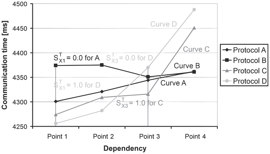
As it was said in the section above, the high-level communication protocol of the distributed road traffic simulations ensures the exchange of traffic information and the synchronization of the simulation. These two tasks can be performed separately, or they can be combined together. In a distributed time-stepped road traffic simulation, the simulation processes are usually synchronized using a barrier. This approach is an instance of a conservative synchronization mechanism. The barrier can be a centralized one, provided by a central control process (e.g., in Ramamohanarao et al., 1 Nagel and Rickert, 4 or Ahmed and Hoque 23 ) or can be a distributed one ensured by all the working processes (e.g., in Ramamohanarao et al., 1 Klefstad et al., 3 or Ventresque et al. 24 ). So, messages necessary for the synchronization are being sent between the control process and the working processes in case of the centralized barrier or among the working processes in case of the distributed barrier. 1 Messages necessary for the transfer of traffic information (i.e., the vehicles and lane-blocks) are being sent between the neighboring working processes (e.g., in Ramamohanarao et al., 1 Klefstad et al., 3 or Nagel and Rickert 4 ). Alternatively, the control process can be used as a message router of these messages (e.g., in Potuzak and Herout 22 or Ahmed and Hoque 23 ). The described possibilities are depicted in Figure 1.
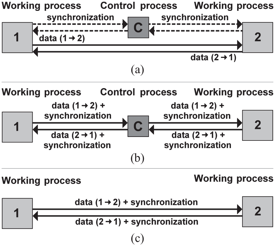
Possible schemes for exchange of message among the control and the working processes: (a) centralized synchronization, distributed vehicle transfer, (b) centralized synchronization, centralized vehicle transfer, and (c) distributed synchronization, distributed vehicle transfer.
3. Related work
Besides our original methodology described in Potuzak, 5 we were unable to find any similar methodology for assessment of high-level communication protocols. However, the performance of general distributed simulations or distributed road traffic simulation is investigated quite often. 5 Existing approaches are briefly described in the following sections.
3.1. General distributed simulation assessment
Several criterions can be used to asses a general distributed simulation. Since the main reason for running a simulation on a distributed computer is to reduce the total computation time, the speedup is the most often used attribute for the performance of the distributed simulation (e.g., in Alian et al., 25 Bononi et al., 26 or Cavitt et al. 27 ). 5
The performance of the distributed simulation is quite often investigated in relation to the size of the model (e.g., in Alian et al., 25 Djemame et al., 28 or Wegener et al. 29 ) and the number of simulation processes (e.g., in Klefstad et al. 3 or Lee et al. 30 ). The number of used simulation processes usually depends on the number of nodes of the distributed computer. Often, there is a one-to-one mapping of the simulation processes to the nodes. 5 In case on nodes with multiple and/or multi-core processors, the processes can be multi-threaded (e.g., in Potuzak 15 ) or there can be one simulation process per processor core. Since the simulation processes must interact throughout the simulation run (see section 2.4), the number of messages sent during the simulation run is also quite often observed. The example is in Ramamohanarao et al. 1
Quite a different approach is described in Fu et al. 31 There, the estimate of a large-scale distributed simulation computation time is based on short sequential simulation runs performed on the same hardware. It is assumed that the distributed computer is homogeneous and the same hardware is used for both the sequential and the distributed simulation runs. 31
Another feature, which can be investigated, is the power consumption. This may be of great importance mostly for mobile devices (which a typical distributed computer is usually not), but it can be a major concern for large-scale distributed computers as well, as a high power consumption can cause high operating costs. Hence, there are also works focusing on the power consumption of distributed simulation, e.g., Fujimoto and Biswas, 32 Biswas and Fujimoto, 33 or Conoci et al. 34 This works indicates the increasing importance of the power usage investigation and control.
3.2. Distributed road traffic simulation assessment
The assessment of the distributed road traffic simulation is very similar to a general distributed simulation (see section 3.1). The speedup of the distributed run in comparison with the sequential run is often the main considered attribute (e.g., in Klefstad et al., 3 Gourgoulis et al., 35 Liu et al., 36 or Mabry and Gaudiot 37 ). The influence of the number of simulation processes and/or the number of nodes of the distributed computer on the performance of the distributed road traffic simulation are also quite commonly investigated (e.g., in Klefstad et al., 3 Gourgoulis et al., 35 or Liu et al. 36 ). 5
Another investigated attribute is the real-time factor. It indicates how many times the simulation is faster than the real-time. It is used, e.g., in Ramamohanarao et al. 1 or Bin Khunayn et al. 38 There are also other attributes, which are investigated less frequently, e.g., the time necessary for the synchronization of the processes, the size of the messages, which are being sent among the simulation processes, or the time necessary to transfer these messages per time step (e.g., in Ramamohanarao et al. 1 ). 5
4. Improved methodology description
In section 3, the approaches and attributes utilized for performance evaluation of entire distributed simulation were described. However, this performance is heavily affected by the performance of the utilized high- and low-level protocols, since the inter-process communication is one of the main bottlenecks of distributed applications in general.5,15
4.1. Measurable parameters of high-level communication protocols
The assessment of the high-level communication protocols can be performed using various measurable parameters. Some parameters were mentioned in section 3. The parameters, which were considered for both the original and the improved methodology, are the number of transferred messages, the number of transferred vehicles and/or lane-blocks, the amount of transferred useful data, the total communication time, and the speedup of the simulation. 5
The number of transferred messages can be determined using a counter of sent messages in each simulation process. The total number of messages sent during the entire simulation run can be then calculated as the sum of the values of the counters at the end of the simulation run. It should be noted that, in most high-level communication protocols, at least a portion of the messages is being sent in a regular manner (e.g., once per time step—usually the synchronization messages). The number of these messages can be easily calculated by the known number of time steps and known number of these messages sent per time step. 5
The number of transferred vehicles and lane-blocks can be determined in a similar manner. Each connecting lane (i.e., the lane leading from a sub-network to a neighboring one) can be equipped by a counter of vehicles and a counter of lane-blocks. The total number of vehicles and lane-blocks can be then calculated as the sum of the corresponding counters at the end of the simulation. 5
The amount of transferred data is more difficult to measure. The reason is that not all implementations of low-level protocols enable to determine the amount of transferred data. Nevertheless, the amount of useful transferred data can be measured in a similar way as the number of messages or vehicles (see above). The amount of useful data can be added to a global counter during the sending of each message. 5 Since the useful transferred data are produced by the high-level communication protocol, it can be assumed that the size of the data is known.
The communication time of the simulation run is difficult to measure. The time, which is easily measurable, is the computation time of the simulation run. The difficult part is to distinguish, which portion of this time is consumed by the simulation itself and which by the inter-process communication. Similar problem is described in Biswas and Fujimoto, 33 but regarding the power consumption. The main reasons are the inaccuracy of the computer clock 39 and the overhead associated with the frequent time measurement. Nevertheless, the computation time can be used as an approximation of the communication time if the inter-process communication is its major portion. This is the case of the simulations of small road traffic networks. For the communication protocol comparison purposes, it is not even necessary to know, how large the portion is if the time consumed by the simulation itself remains approximately constant. This can be achieved by maintaining similar number of vehicles moving within the road traffic network for all the high-level protocols. It is assumed that any effect of the high-level protocols on the course of the simulation is relatively small, because a significant effect would render the protocol useless. In that case, any non-negligible changes in the computation time can be attributed to the change of the communication time. In order to make these changes easily observable, the portion of the computation time consumed by the simulation itself should be minimal. Consequently, an identical very small road traffic network should be used in all comparison tests where the computation time is used as the approximation of the communication time. 5
In comparison to the communication time, the speedup can be determined easily. It can be calculated as the ratio of the sequential and distributed computation time using the equation: 40
where s is the speedup, TS is the computation time of the sequential simulation run, and TD is the computation time of the distributed simulation run. Both simulation runs must be performed on the same hardware (i.e., the sequential version on a single node of the distributed computer). 5 The speedup is closely associated with the efficiency. The efficiency expresses the speedup per node of the distributed computer. It can be calculated using the following equation: 40
where η is the efficiency, s is the speedup, and n is the number of utilized nodes. The higher the efficiency is, the better the simulation is parallelized. The efficiency value of 1.0 corresponds to a linear speedup, meaning that the distributed simulation is two times faster on two nodes. Usually, the efficiency is lower. 5
It should noted that, for all the described measurable parameters, multiple measurements (meaning multiple simulation runs) and averaged mean values must be usually used. Due to the utilization of pseudorandom numbers, even two sequential simulation runs of the same road traffic network with the same input parameters are not identical, and the measured parameters including the number of transferred vehicles and lane-blocks or the number of transferred messages can slightly vary.
There are some exceptions. For the number of transferred messages, a single measurement during a single simulation run is sufficient if all the messages are transferred regularly. The simulation runs of the same road traffic network with the same input parameters can be also rendered identical by careful and constant setting of the seeds of the pseudorandom number generators. This would change the simulation to a deterministic one. Depending on the implementation of the simulation, this may be quite difficult to achieve. For example, it may not be possible to set the seeds of the generators at all or to desired values. Also, there are other sources of variability in the distributed simulations, such as intentional relaxed synchronization of the simulation processes (i.e., a feature of a high-level communication protocol), which may prevent achieving a deterministic simulation run. Moreover, while it may be acceptable for the measurement purposes, it is generally not desirable to use the same seeds in all simulation runs. Different seeds enable to explore greater part of the state space of the simulation and the averaging of the results mitigates random excess values. In addition, for the measurement of the computation time, multiple simulation runs are necessary even when the simulation is deterministic, since other processes of the operating system running on the limited number of processor cores can significantly affect the measurement.
4.2. Attributes influencing high-level communication protocols
The high-level communication protocols and their performance can be influenced by several factors. These factors include the attributes of the simulated road traffic network, the attributes of the distributed simulation, and the attributes of the distributed computer hardware. 5 The fidelity of the high-level protocol in sense of its ability to transfer the vehicles and lane-blocks information with or without an introduced error can also play a significant role.
The attributes of the simulated road traffic network include the number of traffic lanes, which interconnect the individual sub-networks, the vehicle density in these lanes, and the size of the road traffic network. 5 The number of connecting traffic lanes affects the performance of the high-level communication protocol, because the number of vehicles and lane-blocks, which must be transferred between the neighboring sub-networks by the communication protocol, increases with the increasing number of connecting lanes. For this reason, the number of connecting lanes should be minimized already by the division of the road traffic network, which is performed prior the simulation.4,5,41 The number of vehicles, which must be transferred between the neighboring sub-networks, is also affected by the vehicle density in the connecting traffic lanes. Even with a low number of connecting lanes, a high vehicle density in these lanes means a high number of vehicles and lane-blocks, which must be transferred by the communication protocol. In many cases, it can be difficult to avoid the usage of all lanes with high vehicle density as connecting lanes during the road traffic network division, since they can lead through the entire road traffic network. 5 Various high-level communication protocols can cope with increased number of vehicles and lane-blocks to transfer to a varying degree.
The final attribute of the simulated road traffic network affecting the performance of the high-level communication protocol and of the entire distributed simulation is the road traffic network size. The smaller the road traffic network is, the larger portion of the total computation time is consumed by the inter-process communication and the smaller portion is consumed by the simulation itself. For very small road traffic networks, a very low or zero speedup, or even a slowdown can be observed.5,42 Some high-level communication protocols can reduce the time spent by the inter-process communication to a varying degree.
The attributes of the distributed simulation include the number of simulation processes and the low-level communication protocol (implemented in the middleware) ensuring the very message passing. The number of simulation processes significantly influences the resulting speedup of the distributed simulation. Assume now that each simulation process is running on a different node of the distributed computer. Usually, with the increasing number of simulation processes (and utilized nodes), the speedup increases as well. However, the efficiency, which expresses the speedup per node (see section 4.1), usually decreases. In case of distributed road traffic simulations, the decrease can be quite rapid.3,35,37 The main reason is a more intense inter-processes communication caused by a higher number of communicating processes. A higher number of simulation processes leads to a higher number of connecting traffic lanes and, consequently, to a higher number of vehicles and lane-blocks to transfer. 5 In addition, the synchronization of a higher number of processes usually takes more time due to the higher number of synchronization messages and potentially longer waiting for the slowest process. Again, various high-level communication protocols can cope with this problem to a varying degree.
The low-level communication protocol ensuring the message passing can significantly influence the performance of the high-level communication protocol. The low-level communication protocol can be represented by its overhead per message. The overhead per message is the amount of data included in every transferred message, which is necessary for the maintaining of the communication by the low-level protocol, but which are not useful for the simulation itself. Various low-level protocols can have various overheads per message. Since various high-level communication protocols can use very different number of messages, the overhead per message of the low-level communication protocol can significantly affect the resulting performance of the individual assessed high-level communication protocols. 5
The attributes of the distributed computer hardware, where the simulation is performed, include the computing power of individual nodes and the speed of the computer network interconnecting the nodes. These attributes naturally affect the performance of the high-level communication protocol and of the entire distributed simulation. Nevertheless, we assume that most users of the distributed road traffic simulators do not have access to multiple distributed computers with varying attributes. Hence, it would be inconvenient for the methodology to require tests performed on multiple distributed computers. We will not consider this option further. 5
The last attribute—the fidelity of the high-level communication protocol—was not considered in our original assessment methodology, but is considered in its improved version. A high-level communication protocols can be a lossless or a lossy one. 43 A lossless protocol does not introduce an error into the simulation and can be compared to a lossless data compression. A lossy protocol does introduce an error into the simulation and can be compared to a lossy data compression. An error introduced into the simulation by a lossy protocol may be acceptable if the influence on the simulation results is negligible. Hence, the error introduced into the simulation shall be examined. The fidelity of the lossless protocols should be examined as well, because this examination can uncover potential flaws in the implementation of the lossless protocols (see section 4.3).
4.3. High-level communication protocol fidelity testing
Since the fidelity of the high-level communication protocol expresses the error introduced into the simulation, it can be determined from the comparison of the sequential and the distributed simulation runs rather than from the measurable parameters of the high-level communication protocol described in section 4.1. There are multiple ways how to compare the simulation runs. Because the results of the simulation depend mainly on the individual vehicles, the comparison of the positions of all vehicles in each time step seems to be a most precise choice. However, the simulation does not have to support recording of the positions of the vehicles and it may be difficult to add such functionality. In addition, it may be difficult to find corresponding vehicles in two simulation runs—e.g., the vehicles can lack ID or this ID can vary in various simulation runs.
Hence, a more convenient approach will be used in the improved methodology. Instead of position of individual vehicles, the number of vehicles in each traffic lane in each time step can be recorded. This information should be readily available in majority of the simulators, since the numbers of vehicles in individual lanes are a typical statistical result provided by the simulation. The recorded numbers of vehicles can be used for the comparison of two simulation runs. More specifically, the difference of the numbers of vehicles in the ith traffic lane Δli during a sequential and a distributed simulation run can be expressed as follows:
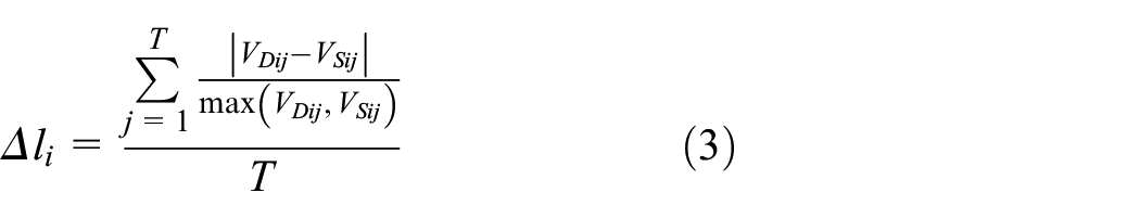
where VSij is the number of vehicles in ith lane in jth time step of the sequential simulation run, VDij is the number of vehicles in ith lane in jth time step of the distributed simulation run, and T is the length of the simulation run in time steps. The total difference d of the entire road traffic network can be then expressed as follows:
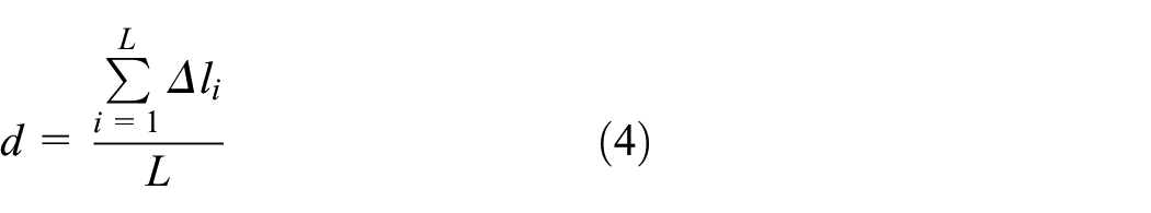
where L is the number of traffic lanes without the connecting lanes. The connecting lanes are not included into the comparison of the simulation runs since they can be divided into two parts in the distributed simulation run.
There is one more issue, however. The stochastic nature of the simulation hampers the exact comparison. Even two sequential simulation runs of the same road traffic network with the same input parameters are not identical due to the utilization of pseudorandom numbers (and possibly other influences—see section 4.1). As stated in section 4.1, it may be possible to render the simulation deterministic by a careful and constant setting of the seeds of the pseudorandom generators. For the fidelity testing, this is a more difficult task, since it is necessary to compare a sequential and a distributed simulation run. The usage of multiple simulation processes for the distributed simulation run means that there are multiple pseudorandom generators in different processes. That must be taken into account. A way how to tackle this issue is to use multiple generators even in the sequential run and based their seeds on the IDs of the elements, for which they generate the pseudorandom numbers. This approach is used in the case study for the fidelity testing (see section 5.2). If the implementation of the simulation and the nature of the tested high-level communication protocols enable the deterministic run, the total difference can be calculated from a single sequential run and a single distributed run. In that case, zero total difference means that no error is introduced into the simulation. The zero total difference should be achieved by the lossless communication protocols. If the implementation of the simulation or the nature of the tested high-level communication protocols do not enable the deterministic run, the total difference should be averaged from multiple simulation runs (similar to the measurement of computation time and other parameters—see section 4.1). In this case, zero value cannot be expected even for the lossless communication protocols. Because it can be expected that many existing simulators do not enable the deterministic run, a small road traffic network should be used for the fidelity testing. In a small road traffic network, all lanes used for the calculation of the total difference are close to the border of the sub-networks and the differences in numbers of vehicles can be attributed mainly to the high-level communication protocol. In greater distances from the border, the influence of the high-level communication protocol can be significantly lower due to the stochastic nature of the non-deterministic simulation runs. A small road traffic network should be sufficient for the testing of the fidelity. As the methodology is designed for micro-scale road traffic simulations, it is expected that the tested high-level communication protocols do not employ any form of lossy information aggregation across more than one connecting traffic lane. As such, the data transferred for various connecting traffic lanes are relatively independent. Hence, adding more connecting lanes due to the usage of a larger road traffic network should not affect the fidelity. In addition, the usage of a small road traffic network keeps the calculation of the total difference fast and simple.
It should be noted that the implementation of the high-level communication protocol can contain various flaws, which can (but does not have to) negatively affect its fidelity in a sense that, without these flaws, the error introduced into the simulation would be lower. The fidelity testing can indicate the presence of such flaws, but only for the lossless protocols and deterministic simulation runs (see above) used for the testing. In that case, the tester can decide whether to disqualify the protocol or to deem the non-zero total difference of a lossless high-level communication protocol acceptable. For lossy protocols and/or non-deterministic simulation runs, it cannot be distinguished, what the cause of the non-zero total difference is.
4.4. Individual dependencies’ testing
As it was described in section 4.2, there are several attributes influencing the performance of the high-level communication protocols. Various protocols can be influenced differently since they can be based on various approaches. It is convenient to test dependency on each attribute in a separate set of tests where only one attribute changes. This way, it is clear how the change of a single attribute affects the performance of the high-level communication protocol. For each dependency testing, a convenient road traffic network(s) shall be used. The improved assessment methodology includes testing of dependencies on four attributes—the number of connecting traffic lanes, the vehicle density in connecting lanes, the size of the road traffic network, and the number of simulation processes (i.e., number of sub-networks).
In the original assessment methodology, all tests were performed with two different low-level communication protocols in order to investigate the influence of the overhead per message. 5 This approach is not used in the improved methodology. Instead, only one low-level communication protocol should be used. If there are multiple available low-level communication protocols, the protocol with the lowest overhead per messages shall be used in order to minimize the communication time. Nevertheless, in many distributed simulations, there is only one available low-level protocol. In such cases, it would be impractical to implement another one if the only reason was the requirements of the assessment methodology. This is one of the reasons why multiple low-level protocols are not required by the improved assessment methodology. The usage of only one low-level protocol also reduces the number of tests for the investigation of individual dependencies to one half. If the investigation of the influence of various low-level communication protocols is required (which is not regarded a common case), the improved methodology can be performed with each of the low-level communication protocols and the results (i.e., the obtained scores—see section 4.5) can be compared.
The performance of the high-level communication protocols should be described primarily by the communication time and the speedup, since the main aim of the utilization of a distributed computer is to reduce the computation time of the simulation. The speedup and the communication or computation time are commonly used for the assessment of the performance (e.g., in Klefstad et al., 3 Gourgoulis et al., 35 Liu et al., 36 or Mabry and Gaudiot 37 ). 5 The number of transferred message should be used as well. It is also used for the assessment of the performance (e.g., in Ramamohanarao et al. 1 ), and it is relatively easily measurable. 5 Other parameters, such as the number of transferred vehicles and lane-blocks or the amount of transferred data (see section 4.1), can be useful as supplementary information and/or for debugging purposes, but are not considered by the improved or the original methodologies. 5
The number of transferred messages was used for all four dependencies. The communication time was used for the dependencies on the number of connecting traffic lanes and on the vehicle density in connecting lanes. For these dependencies, the usage of small road traffic networks makes various performances of the high-level communication protocols more visible while keeping the computation time (and the testing time) low. It also enables to approximate the communication time by the computation time as the simulation itself consumes relatively small portion of the total computation time (see sections 5.3 and 5.4). The speedup was used for the dependencies on the size of the road traffic network and on the number of simulation processes. These dependencies require road traffic network of various sizes and relatively large road traffic network divided into varying number of sub-networks, respectively. Both requirements are necessary to ensure that the testing represents realistic scenarios. The usage of these road traffic networks prevents the usage of the computation time as the approximation of the communication time, because the simulation itself consumes the majority of the computation time. Hence, the speedup is used instead of the communication time (see sections 5.5 and 5.6).
4.5. Individual scores and overall score
In order to enable easy comparison of the performance of the assessed high-level protocols, an overall score for each tested protocol is calculated. The overall score is calculated from the scores each high-level protocol obtains based on the results in the testing of individual dependencies on the attributes described in section 4.4. In the improved methodology, the fidelity score of the high-level communication protocol (see section 4.3) was added to the overall score calculation and the calculation was also slightly changed.
In order to maintain the consistency and simple calculation of the overall score, all the individual scores are in range of <0; 1>. The overall score can be then expressed as follows:

where S is the overall score SF is the fidelity score,
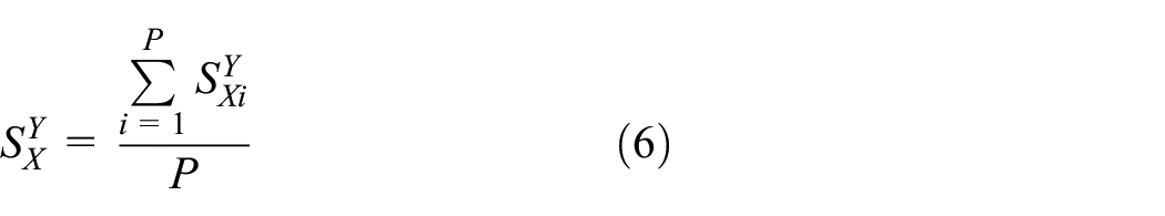
All the fidelity, messages count, communication time, and speedup scores used in Equation (5) are calculated similarly. For each high-level protocol and dependency, there is a curve of the messages count and a curve of the communication time or speedup. Similarly, for the fidelity of the high-level protocol, there is a curve of the total difference (see section 4.3). The curves are constructed from several points, in which the values were measured (or calculated—see Figure 2). The score can be generally expressed as follows:
where
The calculation of the scores for a dependency in points of curves of four protocols.
Assume now that there are communication time curves for a dependency and each curve correspond to one high-level protocol (see Figure 2). The scores in an individual point of the curves represent the mutual comparison of tested high-level protocols. This enables to calculate the score for a dependency of a high-level protocol as the arithmetic mean of the scores in individual points using Equation (6) even when the points represent various numbers of connecting traffic lanes, various vehicle density, and so on. In a point of a curve, the protocol with the worst performance obtains the score of 0.0 and the protocol with the best performance obtains the score of 1.0 (see Figure 2). The protocols with intermediate performances obtain values between 0.0 and 1.0. For the fidelity, messages count, and communication time curves, the lowest value corresponds to the best performance. This situation is depicted in Figure 2. For the speedup curve, the highest value corresponds to the best performance. 5 So, the fidelity score of a high-level communication protocol in ith point can be expressed as follows:
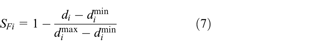
where SFi is the fidelity score in ith point, di is the total difference for a high-level protocol in ith point,
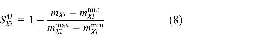
where
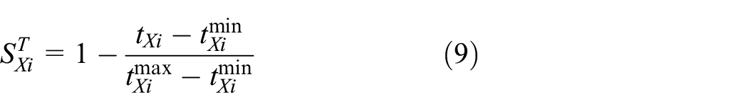
where
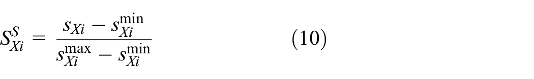
where
From Equations (7)–(10), it is clear that the score in ith point of the curves can be calculated only for multiple communication protocols. Hence, if there is only one high-level communication protocol to assess, another reference high-level communication protocol must be added to enable the score calculation. Such a reference protocol can represent a commonly used protocol in distributed road traffic simulations. The comparison to the reference protocol can show that the assessed high-level communication protocol is better or worse than a commonly used one. Therefore, the usage of the reference high-level communication protocol can be useful even when there are multiple high-level communication protocols to assess. 5
5. Case study: assessment of four protocols with variants
Based on the information in section 4, the individual sets of tests for the complex assessment of the high-level communication protocols can be specified. To demonstrate the functioning of the improved methodology, the tests were performed on three high-level communication protocols of our own design (each with three variants) and one reference high-level communication protocol (see section 5.1).
The tests were performed using the DUTS (Distributed Urban Traffic Simulator), which was developed at Department of Computer Science and Engineering (DCSE) of University of West Bohemia (UWB). For the tests, only one of the three micro-scale road traffic models available in DUTS 6 —the Java Urban Traffic Simulator (JUTS)–based model—was used for the testing, since the utilized road traffic model has little effect on the high-level communication protocols.5,38 The DUTS incorporates two low-level communication protocols—the RMI 21 and the TCP. 20 Only the TCP, which shows lower overhead per message, was used for the testing. The testing was performed on Hydra cluster, which is available at DCSE UWB. The cluster contains 10 nodes interconnected with a standard 1 Gbit Ethernet utilized for the message passing among the simulation processes. Each node incorporates an Intel Xeon CPU at 3.2 GHz and 2 GB of RAM. There was one simulation process per node including the control process. So, from three to nine nodes were used for the distributed simulation runs. A single node of the cluster was used for the sequential runs when necessary.
5.1. Assessed high-level communication protocols
As it was stated in section 5, there were three high-level communication protocols, which we developed during our past research—the Long Step (LS), the Long Step Characteristics (LSC), and the Long Step Binary (LSB) protocols. Each protocol has three variants. In the Semi-Centralized (SC) variants, a centralized barrier is employed for the synchronization. So, the synchronization messages are transferred between the control process and the working processes simulating individual sub-networks. The messages with vehicles and lane-blocks are transferred directly between the neighboring sub-networks (see Figure 1(a)). In the centralized (C) variants, the vehicles and lane-blocks are transferred added to the synchronization messages, and the control process acts as a message router (see Figure 1(b)). In the distributed (D) variants, a distributed barrier is employed for the synchronization. So, the synchronization messages are transferred among the neighboring working processes. The vehicles and lane-blocks are added to these messages (see Figure 1(c)). In addition, there is a reference protocol with only one variant—the Semi-Centralized Single Vehicle (SC-SV) protocol.
The LS protocol is a lossless high-level communication protocol, since it transfers the vehicles and lane-blocks precisely, and no error is introduced into the simulation. All the variants reduce the number of transferred messages using the long step technique.5,22,43 That means that both the synchronization and the transfer of vehicles and lane-blocks are performed only once per several time steps. The number of steps between two successive synchronizations is called the long step and can be set prior the start of the simulation.22,43 For the tests described in section 5, the length of the long step is set to eight steps. In addition, the number of transferred messages is further reduced by sending multiple vehicles and lane-blocks within a single message. In the SC-LS variant, there is single message with vehicles and lane-blocks per neighboring process per long step. In the C-LS and D-LS variants, there are no separate messages with vehicles and lane-blocks at all. Instead, the vehicles and lane-blocks are transferred within the synchronization messages22,43 (for the detailed description of the LS protocol, see Potuzak and Herout 22 and Potuzak 43 ).
The LSC protocol is a lossy high-level communication protocol. It is based on the transfer of characteristics of traffic flow (specifically, the vehicle density and the mean speed) instead of vehicles. This reduces the amount of transferred data, but for the price of an error introduced into the simulation.5,44 The LSC protocol also transfers multiple characteristics and lane-blocks within a single message and employs the long step technique much like the LS protocol. Hence, the only difference in comparison to the LS protocol is the usage of the characteristics of traffic flow instead of the vehicles (for detailed description of the LSC protocol, see Potuzak 44 ).
The LSB protocol is a lossy high-level communication protocol. It is very similar to the LSC protocol—it is based on the transfer of characteristics of traffic flow as well.5,6,43 However, the vehicle density is replaced by binary-encoded positions of the transferred vehicles. This leads to a diminishment of the error introduced into the simulation (i.e., to an improvement of the fidelity of the protocol). Similar to both previous protocols, the LSB protocol transfers multiple characteristics and lane-blocks within a single message and employs the long step technique (for detailed description of the LSB protocol, see Potuzak6,43).
The SC-SV reference protocol is a lossless high-level communication protocol, which transfer each single vehicle or lane-block in a separate message. 43 It has only one variant (SC). It utilizes a centralized barrier provided by the control process for the synchronization. The synchronization is performed in every time step. The messages with individual vehicles and lane-blocks are transferred directly between the neighboring working processes (see Figure 1(a)). This protocol is quite commonly used (e.g., in Klefstad et al. 3 ), although it does not employ any reduction of the number of messages or the amount of transferred data. 43
5.2. Fidelity testing
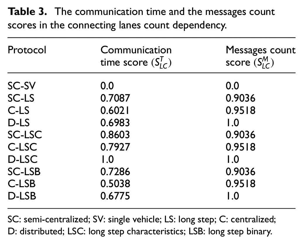
First step of the improved assessment methodology is the investigation of the fidelity of the tested high-level communication protocols. For the assessment of the fidelity, the total difference of the numbers of vehicles in traffic lanes during the simulation run d (see section 4.3) was used. For the tests, a small road traffic network (see section 4.3) with four crossroads was used. The network was divided into two and four sub-networks (see Figure 3). This leads to a different number of compared lanes in these two cases (see Figure 3), but this is not problematic, because the total difference is calculated for each case separately for all tested high-level communication protocols (see Table 1). Each sub-network was simulated by a working process running on a single node of the distributed computer. This configuration was used for all the remaining tests as well. Since the DUTS system enables to set the seeds of pseudorandom generators to constant numbers based on IDs of the elements, for which they generate the pseudorandom numbers (rendering the simulation run deterministic—see section 4.3), only a single sequential run and a single distributed simulation runs per test were performed. Each test corresponds to a combination of the number of sub-networks and of a variant of a high-level communication protocol. Each simulation run was 900 time steps long (corresponding to 900 s or 15 min). This length is derived from the time interval, to which recorded real traffic densities are aggregated in Pilsen city. This way, the results from the simulation runs can be easily compared to the recorded values. 5
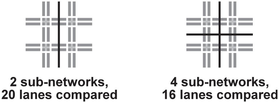
The road traffic network for the fidelity testing.
The total differences of the tested protocols.
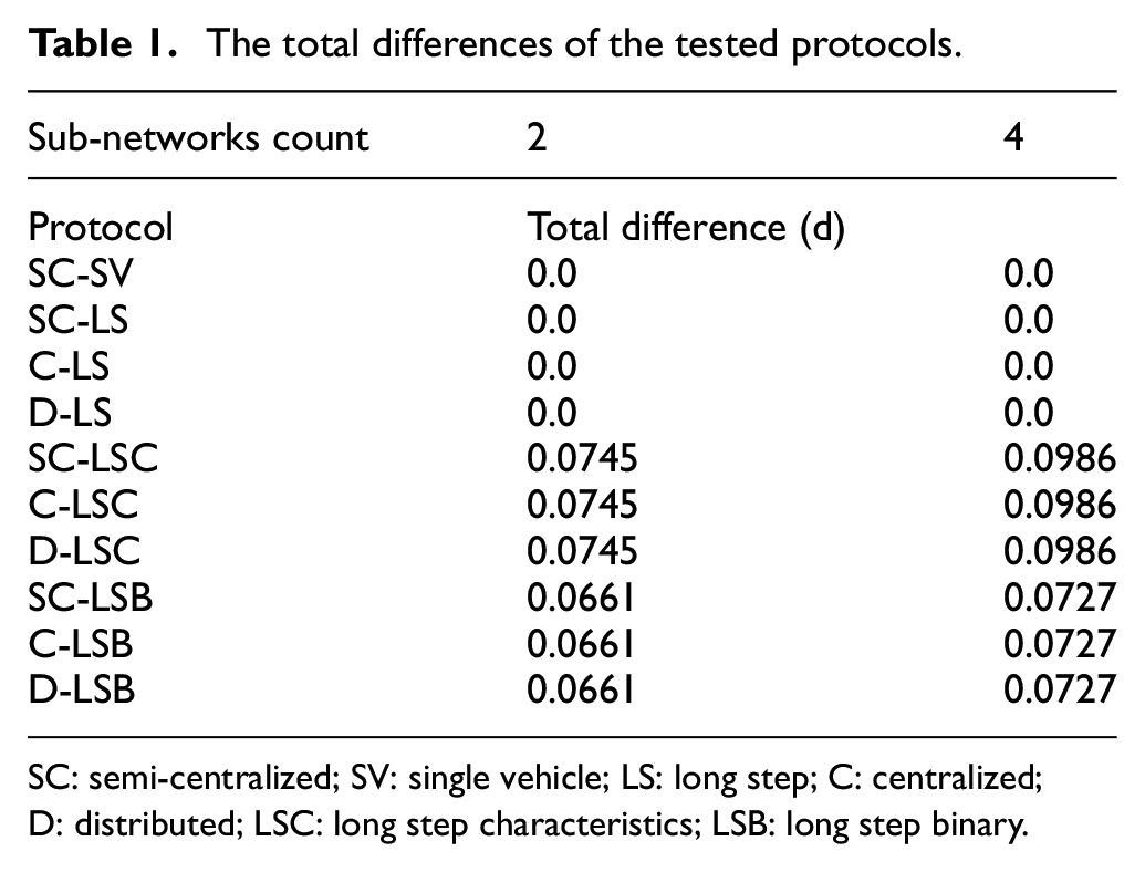
SC: semi-centralized; SV: single vehicle; LS: long step; C: centralized; D: distributed; LSC: long step characteristics; LSB: long step binary.
The resulting total differences for the individual tested high-level protocols were calculated using Equations (3) and (4) and are summarized in Table 1. It can be observed that the lossless communication protocols (the SC-SV reference protocol and all three variants of the LS protocol) show zero total differences, which is an expected and desired behavior. Also, all three variants of the same protocol show the same total difference. That means that, how the vehicles or characteristics and lane-blocks are arranged within the messages, does not influence the simulation. Again, this is an expected and desired behavior. Another observation is that the total differences of the lossy protocols are quite low (maximal theoretical value is 1.0) and the LSB protocol shows lower total difference than the LSC protocol. Since the reason for the development of the LSB protocol was to improve the fidelity of the characteristics-based protocols (see section 4.1 and Potuzak 6 ), this is again an expected behavior.
The fidelity scores for the tested high-level protocols were calculated using Equations (7) and (6) and are summarized in Table 2. Due to the nature of Equations (7) and (6), the different numbers of compared lanes do not affect the calculated fidelity scores (see section 4.5). As can be seen, the lossless communication protocols received the highest and equal scores, while the LSC protocol received the lowest score, since it shows the highest total difference in all instances. The LSB protocol also received low score, since its total difference values are quite close to the values of the LSC protocol.
The fidelity scores of the tested protocols.
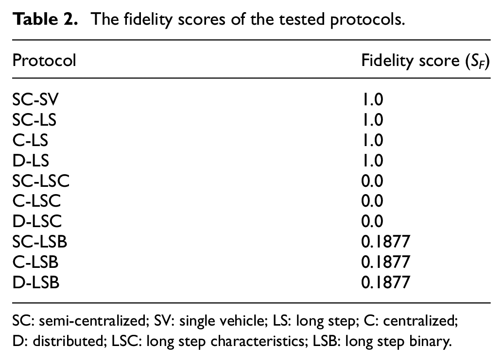
SC: semi-centralized; SV: single vehicle; LS: long step; C: centralized; D: distributed; LSC: long step characteristics; LSB: long step binary.
5.3. Traffic lanes count dependency testing
Next step of the improved methodology is the investigation of the individual dependencies, starting with the dependency of the high-level communication protocol performance on the number of connecting traffic lanes. For the assessment of this dependency, the communication time and the number of transferred messages were used. For the tests, a small road traffic network with 32 crossroads arranged in two rows was used (see Figure 4). The road traffic network was divided into two sub-networks between the two rows. The number of connecting lanes was being changed during the testing and ranged from 2 to 32. The vehicle density in the connecting lanes was roughly constant at 0.25 vehicles per time step (vpts). The usage of a small road traffic network enables to approximate the observed communication time with the computation time and has no negative effects on the investigated dependency. Each test corresponds to a combination of a number of connecting lanes and of a variant of a high-level communication protocol. For each test, 10 distributed simulation runs were performed, and the results were averaged. Each simulation run was again 900 time steps long (see section 5.2). Before the measurement was started, 900 time steps were performed in order to fill the road traffic network with vehicles. This arrangement was used for the remaining dependencies as well.

The road traffic network for the connecting lanes count dependency testing.
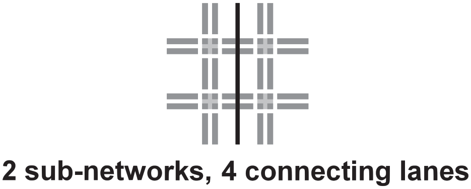
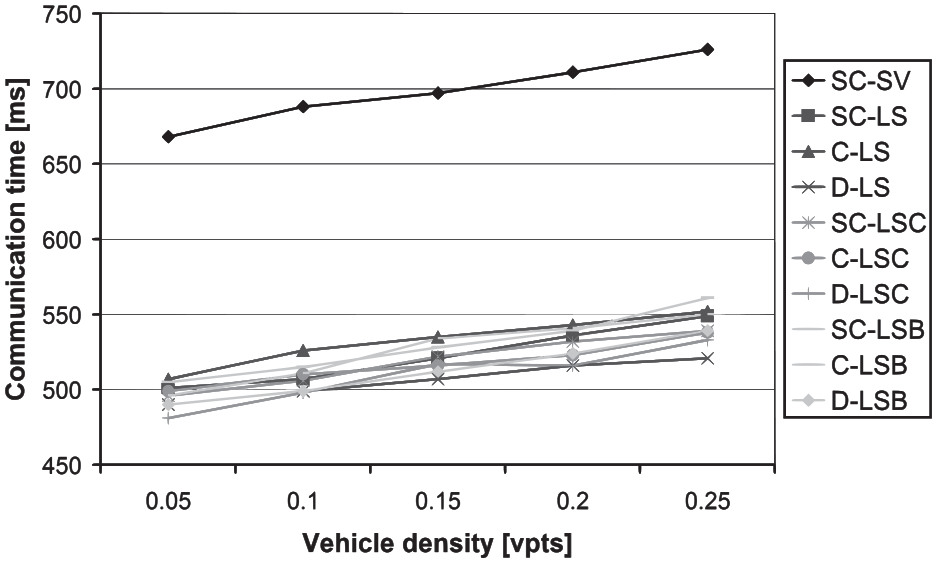
The resulting communication times of the tested high-level protocols are depicted in Figure 5. It can be observed that the communication time increases with increasing number of connecting traffic lanes. This is an expected behavior, since more connecting lanes mean a higher number of vehicles and lane-blocks to transfer. Another observation is that the reference SC-SV protocol shows by far the worst communication time. This is caused by the far larger number of transferred messages, which can be observed in Figure 6.
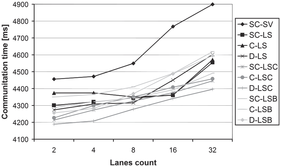
The communication times dependency on the connecting lanes count.
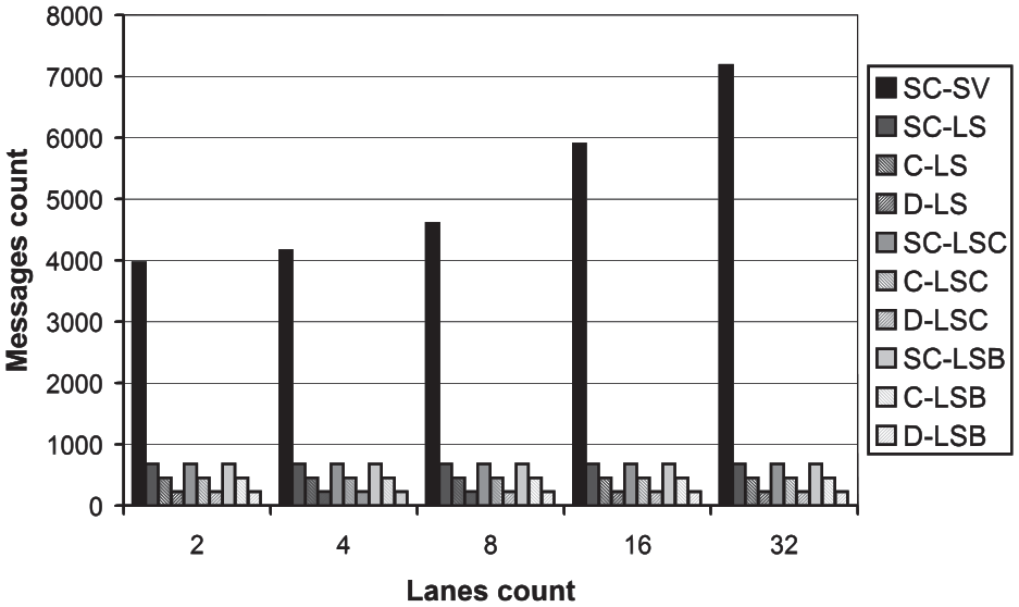
The messages count dependency on the connecting lanes count.
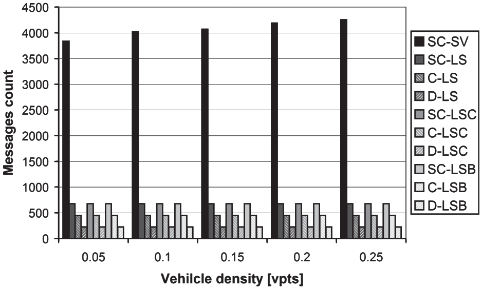
The communication time and the messages count scores were calculated using Equations (9) and (8), respectively. They are summarized in Table 3. It can be seen that the reference SC-SV protocol obtained the lowest scores, since it shows both the highest communication time and the highest number of messages in all instances. The variants of the remaining high-level communication protocol are more balanced in the communication time. The perfect score (1.0) was obtained by the D-LSC variant, since it had the lowest communication time in all instances, but only narrowly. All the distributed variants of the protocols received the perfect messages count scores, since they equally show the lowest number of transferred messages in all instances.
The communication time and the messages count scores in the connecting lanes count dependency.
SC: semi-centralized; SV: single vehicle; LS: long step; C: centralized; D: distributed; LSC: long step characteristics; LSB: long step binary.
5.4. Vehicle density dependency testing
For the assessment of the dependency of the high-level communication protocols performance on the vehicle density in connecting traffic lanes, the communication time and the messages count were again used. For the tests, a small road traffic network with only four crossroads was used (see Figure 7). The road traffic network was divided into two sub-networks. The vehicle density in the four connecting traffic lanes was being changed during the testing and ranged from 0.05 to 0.25 vpts. Again, the usage of a small road traffic network enables to approximate the observed communication time with the computation time and has no negative effects on the investigated dependency. Each test corresponds to a combination of a vehicle density and of a variant of a high-level communication protocol. For each test, 10 distributed simulation runs were performed, and the results were averaged.
The road traffic network for the vehicle density dependency testing.
The resulting communication times of the tested high-level protocols are depicted in Figure 8. It can be seen that the communication time increases with increasing vehicle density in the connecting traffic lanes. Again, this is an expected behavior, since a higher vehicle density in connecting lanes means a higher number of vehicles and lane-blocks to transfer. The reference SC-SV protocol communication time is again the highest by a substantial margin in comparison with the remaining high-level communication protocol variants. Similar to the connecting lanes count dependency, it is caused by the far larger number of transferred messages (see Figure 9).
The communication times dependency on the vehicle density in connecting lanes.
The messages count dependency on the vehicle density in connecting lanes.
The communication time and the messages count scores were again calculated using Equations (9) and (8), respectively. They are summarized in Table 4. Again, the reference SC-SV protocol obtained the lowest scores. The variants of the remaining high-level communication protocol are more balanced in the communication time. This time, no variant obtained the perfect communication time score, because no variant had the lowest communication time in all instances. Again, all the distributed variants of the protocols received the perfect messages count scores because of the lowest number of transferred messages in all instances.
The communication time and the messages count scores in the vehicle density dependency.
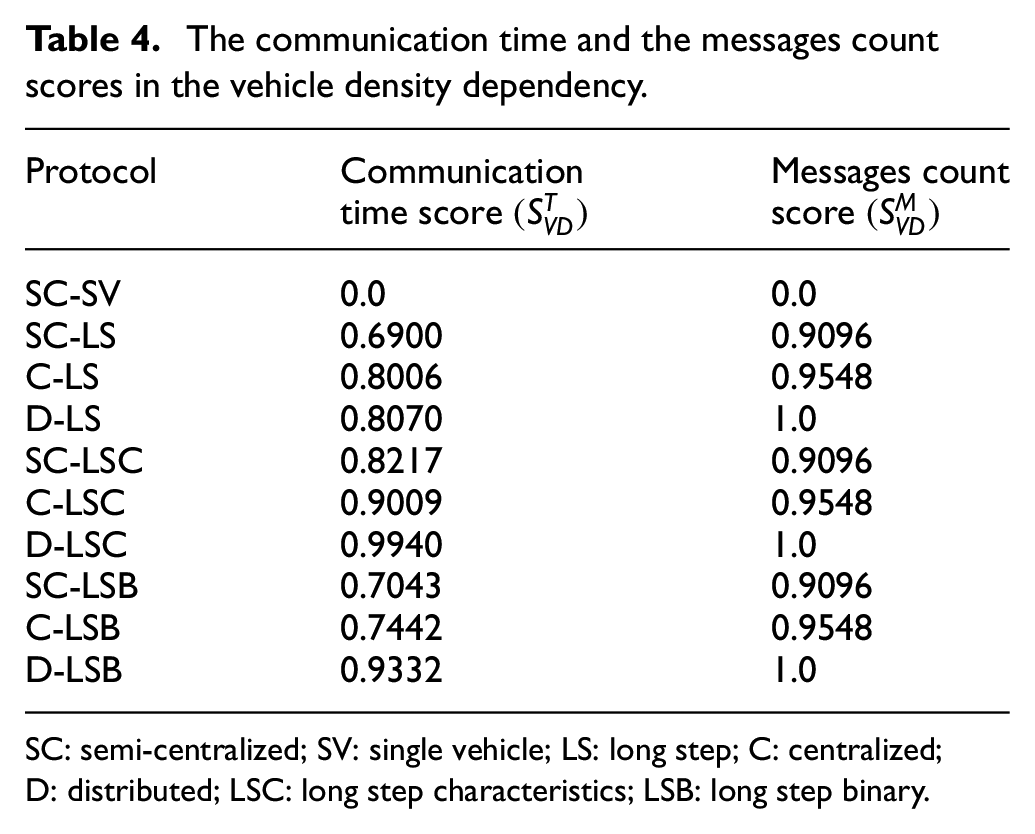
SC: semi-centralized; SV: single vehicle; LS: long step; C: centralized; D: distributed; LSC: long step characteristics; LSB: long step binary.
5.5. Road traffic network size dependency testing
For the assessment of the dependency of the high-level communication protocols performance on the road traffic network size, the speedup and the messages count were used. The speedup was used instead of the communication time since the nature of this set of tests does not allow usage of a small road traffic network of a constant size. On the contrary, three road traffic networks of various sizes were used for the tests. The networks were regular square grids of 16, 64, and 256 crossroads (se Figure 10). Each road traffic network was divided into two sub-networks. Each test corresponds to a combination of a road traffic network and of a variant of a high-level communication protocol. For each test, 10 distributed and 10 sequential simulation runs were performed, and the results were averaged. The sequential runs were necessary for the calculation of the speedup using Equation (1). The computation times used for the calculation of the speedup are summarized in Table 5.
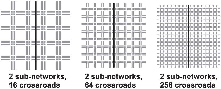
The road traffic network for the road traffic network size dependency testing.
The computation times used for the speedup for the road traffic network size dependency testing.
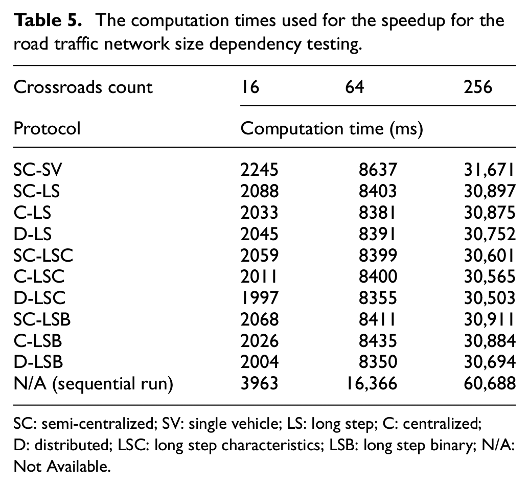
SC: semi-centralized; SV: single vehicle; LS: long step; C: centralized; D: distributed; LSC: long step characteristics; LSB: long step binary; N/A: Not Available.
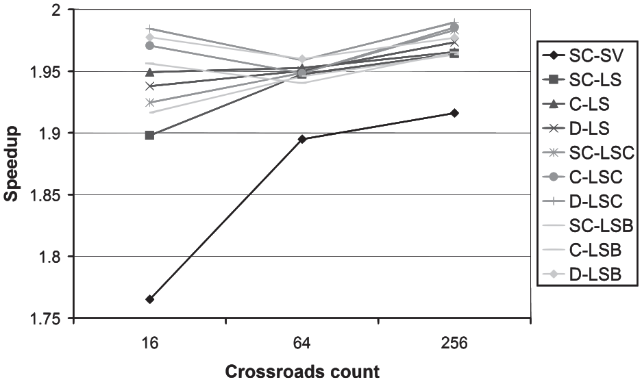
The resulting speedups of the tested high-level protocols are depicted in Figure 11. It can be observed that, for most variants of the high-level protocols, the speedup increases with increasing size of the road traffic network. This is a natural behavior. For a larger road traffic network, a larger portion of the computation time is consumed by the simulation itself and a smaller portion is consumed by the transfer of messages. Nevertheless, four variants (D-LSC, SC-LSB, C-LSB, and D-LSB) show the lowest speedup for the medium road traffic network, which is an unexpected anomaly. However, since this work is focused on the methodology, not the communication protocols themselves, a detailed investigation is outside the scope of this paper. Similar to the previous dependencies, the reference SC-SV protocol shows worst results, this time in the form of the lowest speedup. The cause is again the enormous number of messages transferred by this protocol (see Figure 12).
The speedup dependency on the road traffic network size.
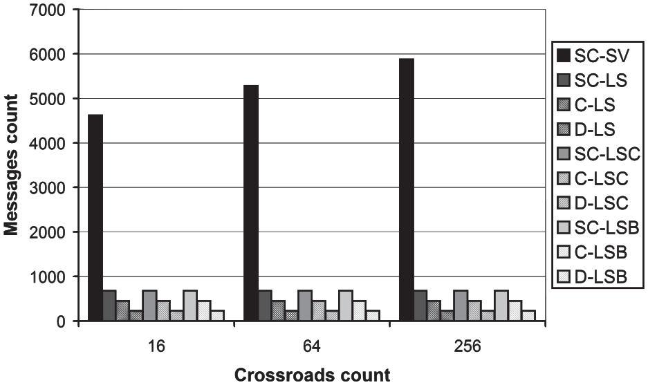
The messages count dependency on the road traffic network size.
The speedup and the messages count scores were calculated using Equations (10) and (8), respectively. They are summarized in Table 6. Again, the reference SC-SV protocol obtained the lowest scores. No variant obtained the perfect speedup score, because no variant had the highest speedup in all instances. Again, all the distributed variants of the protocols received the perfect messages count scores because of the lowest number of transferred messages in all instances.
The speedup and the messages count scores in the road traffic network size dependency.
SC: semi-centralized; SV: single vehicle; LS: long step; C: centralized; D: distributed; LSC: long step characteristics; LSB: long step binary.
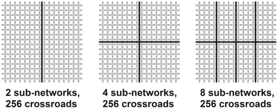
5.6. Processes count dependency testing
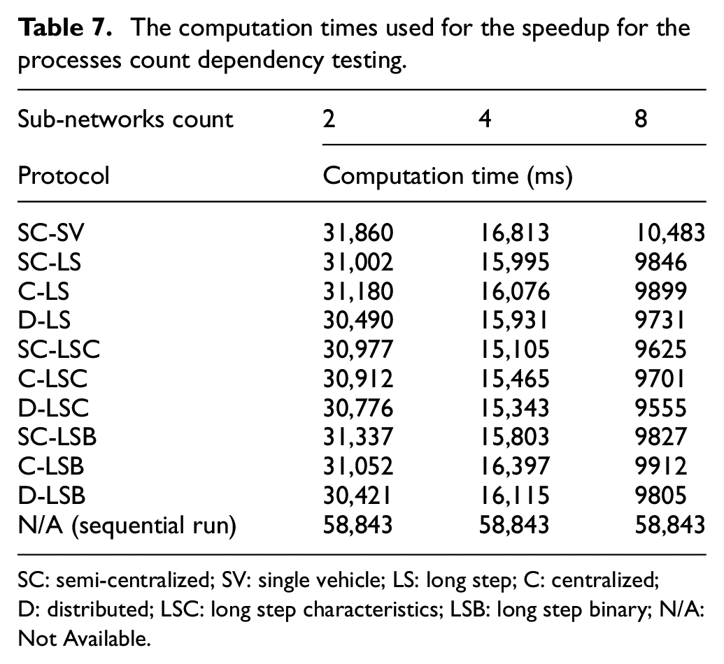
For the assessment of the dependency of the high-level communication protocols performance on the number of working processes, the speedup and the messages count were used. Again, the speedup was used instead of the communication time since the nature of this set of tests does not allow usage of a small road traffic network. For the tests, a regular square grid of 256 crossroads was used (see Figure 13). The network was divided into two, four, and eight sub-networks. Similar to all previous tests, each sub-network was simulated by a working process performed on a single node of the distributed computer. Each test corresponds to a combination of a number of sub-networks (i.e., number of working processes and nodes) and of a variant of a high-level communication protocol. For each test, 10 distributed and 10 sequential simulation runs were performed, and the results were averaged. The sequential runs were again necessary for the calculation of the speedup using Equation (1). The computation times used for the calculation of the speedup are summarized in Table 7.
The road traffic network for the processes count dependency testing.
The computation times used for the speedup for the processes count dependency testing.
SC: semi-centralized; SV: single vehicle; LS: long step; C: centralized; D: distributed; LSC: long step characteristics; LSB: long step binary; N/A: Not Available.
The resulting speedups of the tested high-level protocols are depicted in Figure 14. It can be observed that, for all the variants of the high-level protocols, the speedup increases with the increasing number of processes/nodes. This is an expected and desired behavior, as more nodes offer a larger computing power. Nevertheless, a higher number of processes also mean a higher number of transferred messages (see Figure 15). The increasing number of transferred messages negatively influences the resulting efficiency (see Figure 16). This is also a natural, although not desired behavior. Similar to the previous dependencies, the reference SC-SV protocol shows worst results.
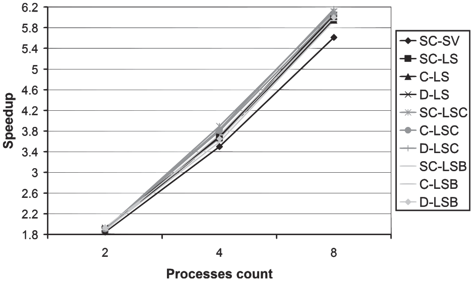
The speedup dependency on the processes count.
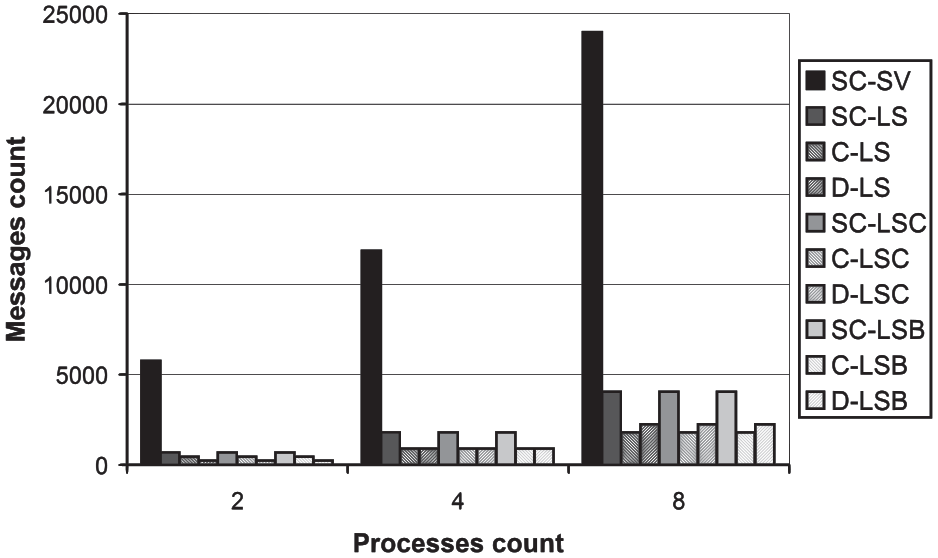
The messages count dependency on the processes count.
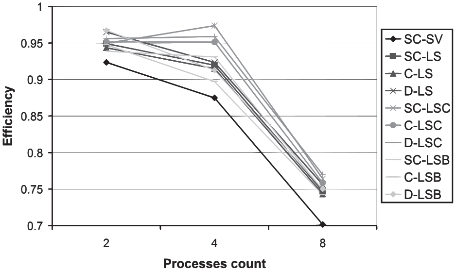
The efficiency dependency in the processes count.
The speedup and the messages count scores were again calculated using Equations (10) and (8), respectively. They are summarized in Table 8. Again, the reference SC-SV protocol obtained the lowest scores. No variant obtained the perfect speedup or messages count scores, because no variant had the highest speedup or the lowest number of transferred messages in all instances.
The speedup and the messages count scores in the processes count dependency.
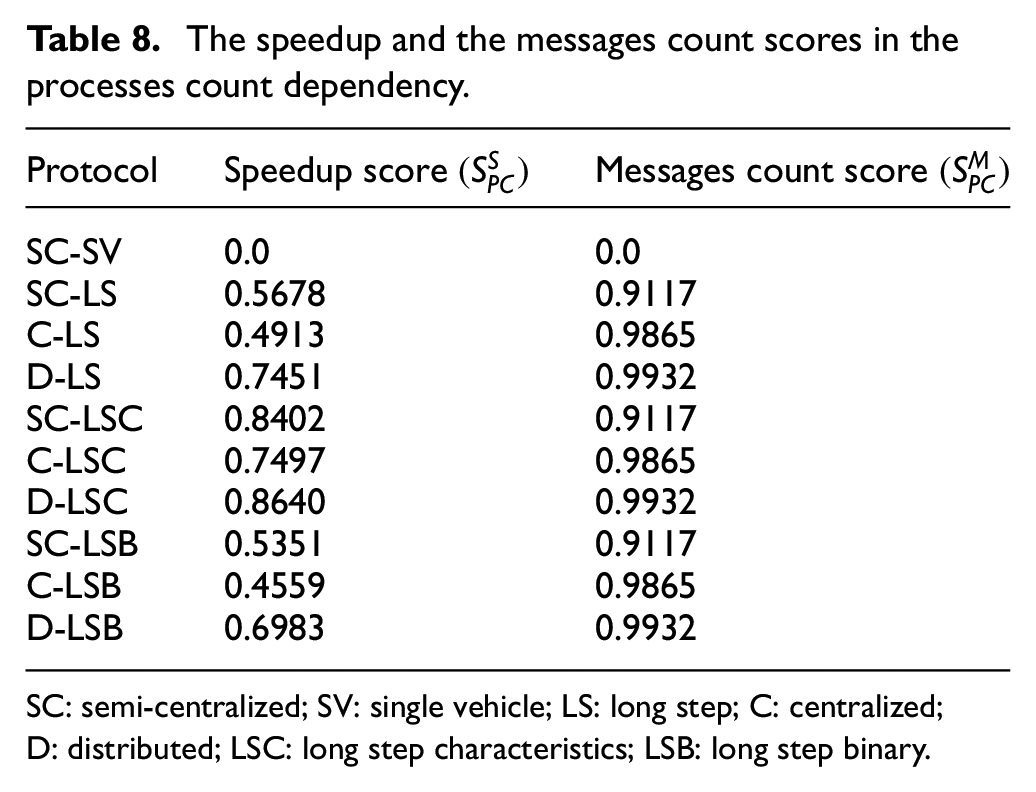
SC: semi-centralized; SV: single vehicle; LS: long step; C: centralized; D: distributed; LSC: long step characteristics; LSB: long step binary.
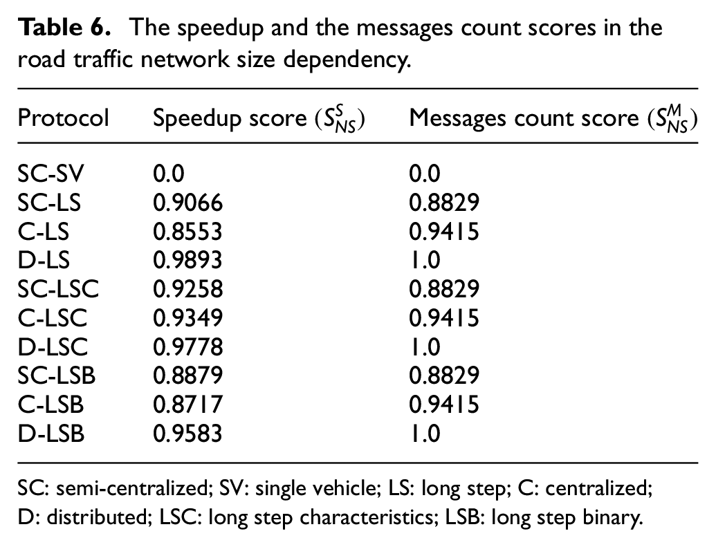
5.7. Overall score calculation
Once all the dependencies were investigated and the corresponding communication time or speedup scores and the messages count scores calculated, it is possible to calculate the overall scores for individual high-level protocols using Equation (5). For the calculation, all weights were set equally to 1.0. The resulting scores are summarized in Table 9.
The overall scores of the assessed protocols.
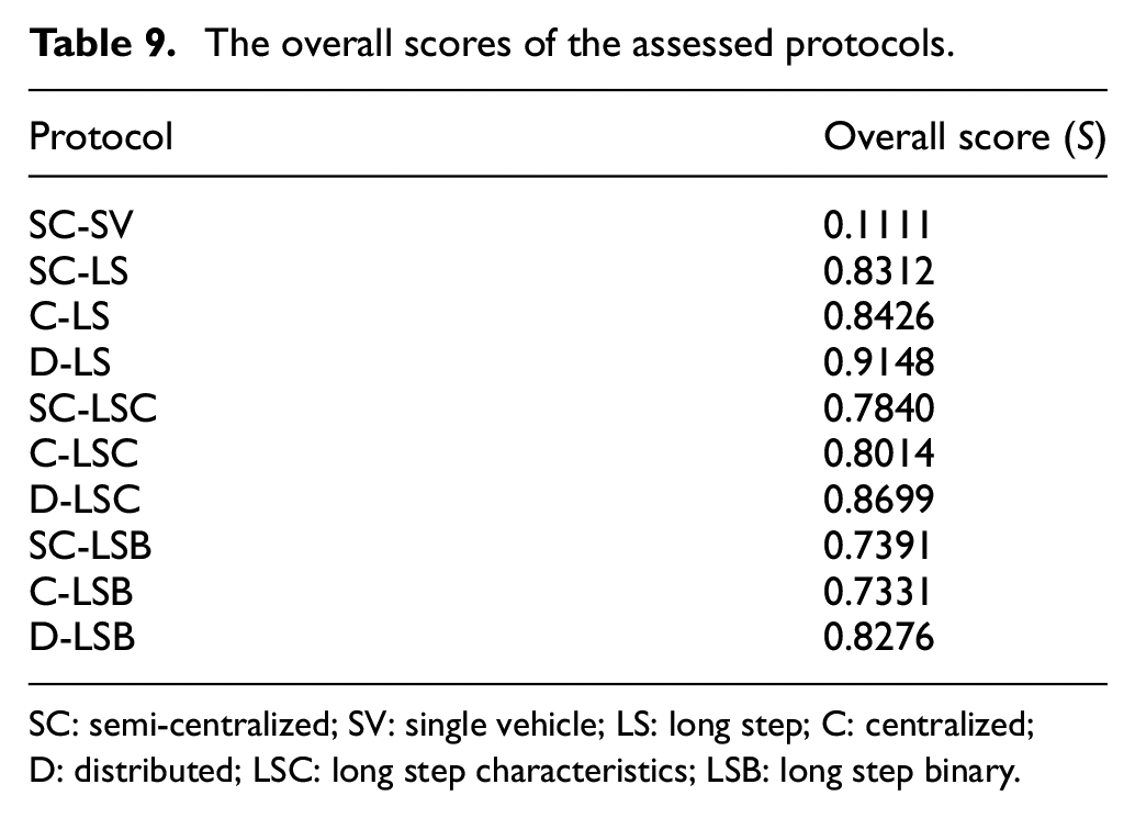
SC: semi-centralized; SV: single vehicle; LS: long step; C: centralized; D: distributed; LSC: long step characteristics; LSB: long step binary.
As can be seen in Table 9, the protocol with the highest overall score is the D-LS. From all the assessed high-level communication protocols, it should ensure the best performance of the distributed road traffic simulation. Also, it is a lossless communication protocol. So, it does not introduce an error into the simulation. The fidelity of the D-LS protocol is the reason, why the protocol obtained a significantly higher overall score that its lossy counterparts (i.e., the D-LSC and D-LSB protocols). The lowest overall score was obtained by the SC-SV reference protocol. The only feature, which elevated its score from zero, was its fidelity.
6. Conclusion and future work
In this paper, an improved methodology for a complex assessment of high-level communication protocol for distributed road traffic simulation was described. It is based on the original methodology described in Potuzak 5 in detail, but reduces the number of performed tests and incorporates assessment of the fidelity of the tested protocols. Also, the calculation of overall scores of the tested protocols was simplified. Using the scores, the tested protocols can be directly compared. This can be useful when designing or improving a distributed road traffic simulation as the best protocol can be used in this simulation to improve its performance (e.g., speedup or communication time). The functioning of the improved methodology was showed on the assessment of three high-level protocols (each with three variants) of our own design and a reference high-level communication protocol. Nevertheless, the methodology can be used for assessment of the high-level communication protocols for micro-scale (or microscopic) distributed road traffic simulation of other parties as well.
In our future work, we plan to use the improved methodology for assessment of other existing third-party high-level communication protocols for distributed road traffic simulations in order to find the one with the best performance. This will also further show the usability of the improved methodology. We will also focus on adaptation of the methodology for other communication protocols outside the field of distributed road traffic simulation.
Footnotes
Funding
The author(s) disclosed receipt of the following financial support for the research, authorship, and/or publication of this article: This work was supported by institutional support for long-term strategic development of research organizations.