
Abstract
Agent-based modeling is a simulation method in which autonomous agents interact with their environment and one another, given a predefined set of rules. It is an integral method for modeling and simulating complex systems, such as socio-economic problems. Since agent-based models are not described by simple and concise mathematical equations, the code that generates them is typically complicated, large, and slow. Here we present Agents.jl, a Julia-based software that provides an ABM analysis platform with minimal code complexity. We compare our software with some of the most popular ABM software in other programming languages. We find that Agents.jl is not only the most performant but also the least complicated software, providing the same (and sometimes more) features as the competitors with less input required from the user. Agents.jl also integrates excellently with the entire Julia ecosystem, including interactive applications, differential equations, parameter optimization, and so on. This removes any “extensions library” requirement from Agents.jl, which is paramount in many other tools.
1. Introduction
Many processes in biology, ecology, sociology, and economics are characterized by interactions between their constituent parts.1–9 A large number of interactions lead to numerous possible states within each system. Such systems, with many interacting components, are complex, where a single component cannot generally determine the system behavior. Each component may have a negligible effect in isolation, but a significant effect when interacting with other components.
To model and analyze complex systems, bottom-up approaches such as agent-based simulations are common, and sometimes the only feasible approach. Agent-based models (ABMs) consist of autonomous agents or individuals that behave according to a set of predefined rules. The rules specify how agents interact with one another, as well as with their environment.
ABMs differ from other analytical models such as differential equations. Analytical models use variables that characterize the whole system, they are top-down. ABMs use variables that describe the components of a system, rather than the behavior of the whole system. A modeler chooses ABM variables based on the understanding of the system, but not to fit some expectations of outcome. The outcome emerges 10 from all these lower-level interactions, which are often nonlinear and cannot be captured by aggregating them. By incorporating spatial and temporal heterogeneity, each agent may only interact with a local neighborhood. Such heterogeneity allows for more realistic models that can show behaviors not captured in top-down approaches. 11
An agent-based modeling framework helps define a general structure for ABMs. Reducing the amount of code needed to write an ABM, and providing a standardized model template, makes it easier for model developers to define models, explore parameters, and collect data, as well as enabling the target audience to better understand, compare, reproduce, and modify models (Figure 1). This is especially important at present, since increasingly complex models are being developed in collaboration, where each party focuses on a single component of the model. A well-defined and simple framework fosters mutual understanding between collaborators. ABMs can be computationally heavy programs, and implementing one from scratch that “works” is seldom “fast” the first time around. A well-designed agent-based simulation framework has taken care of the largest performance bottlenecks one may encounter as much as possible. Such a framework also separates the tasks of defining a model from running it, collecting and merging model outputs, and analysing the results.
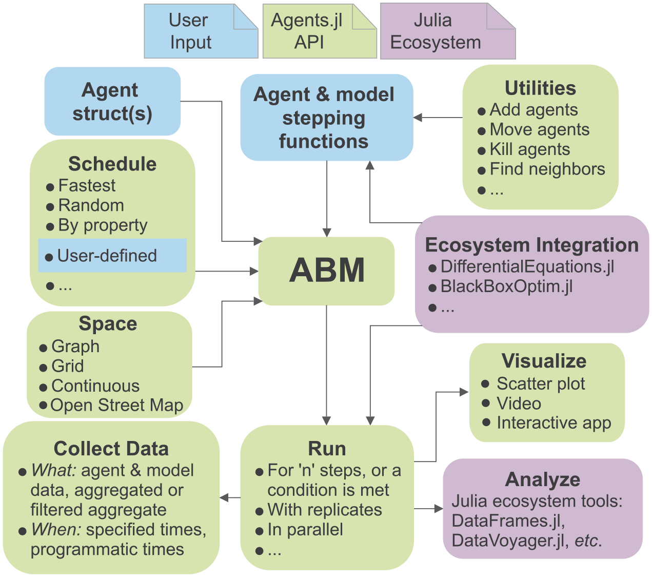
Flow chart representation of the Agents.jl framework.
We developed an agent-based simulation framework, Agents.jl, 12 that fulfills the aforementioned tasks. Various agent-based simulation frameworks exist in different programming languages. 13 Notable examples include Swarm, 14 NetLogo, 15 MASON, 16 Repast, 17 and Mesa 18 (for a comprehensive review, see Abar et al. 19 ). These frameworks differ in their capabilities, scope, learning curve, amount of code needed to develop a model, speed of execution, and data collection and visualization features. Our framework is written purely in the Julia language. This programming language choice brings advantages over other frameworks: quick and intuitive model development, fast model execution, and easy integration with many analytical tools in the Julia ecosystem (removing the need for plugins or extensions). Finally, because Julia is a general purpose language, coding skills developed while learning and working with Agents.jl are directly transferable to other situations outside ABMs (while this is in contrast with, for example, NetLogo, which is mostly a GUI-based, isolated piece of software).
Here we discuss Agents.jl 20 version 4, with many more features and improvements over the initial release. Specifically, it supports three additional space types (continuous space, directed graphs, and OpenStreetMap), better visualization functions, more flexible data collection, simpler source code, automatic parameter exploration, and interactive model execution and visualization. We show the advantages of Agents.jl through a detailed comparison with three other commonly used frameworks: Mesa, NetLogo, and MASON (Tables 1 and 2 and comparison section). We also demonstrate its integration with other Julia packages to create powerful applications, including differential equations in ABMs, optimization of model parameters, and construction of novel space types.
A comparison of four ABM frameworks covering the objective and subjective categories focusing on ease of use, available functionality, and performance.
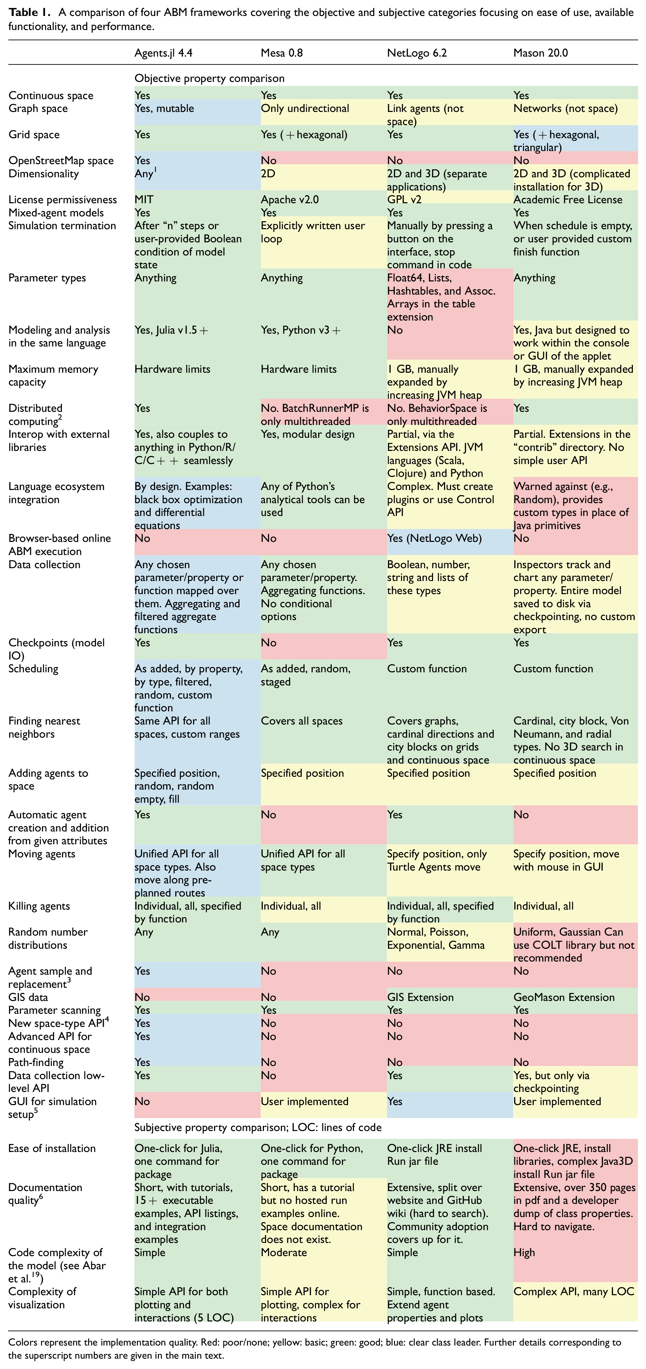
Colors represent the implementation quality. Red: poor/none; yellow: basic; green: good; blue: clear class leader. Further details corresponding to the superscript numbers are given in the main text.
Benchmarks of four model types across four ABM frameworks.
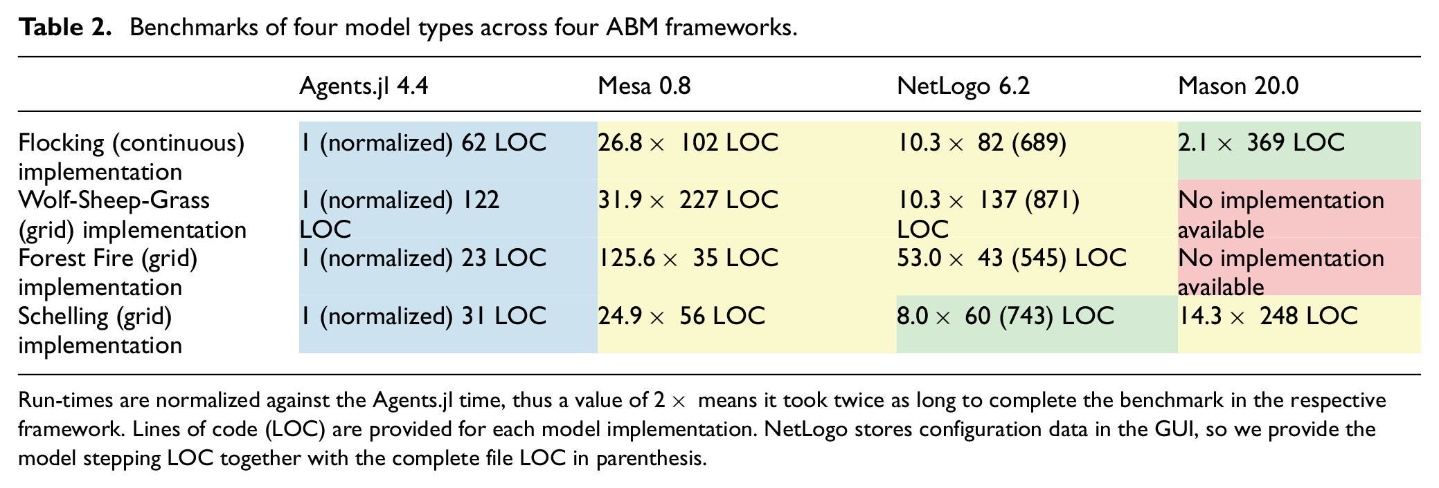
Run-times are normalized against the Agents.jl time, thus a value of 2× means it took twice as long to complete the benchmark in the respective framework. Lines of code (LOC) are provided for each model implementation. NetLogo stores configuration data in the GUI, so we provide the model stepping LOC together with the complete file LOC in parenthesis.
2. Simulations with Agents.jl
The design of Agents.jl separates a simulation into simple components, following the philosophy of giving as much freedom to the user as possible while also minimizing the usage complexity. Each of these components integrates with each other through the help of the Agents.jl API, as illustrated in Figure 1. In this section, we will describe the design of Agents.jl, by going through a typical workflow of an Agents.jl simulation, referencing all aspects of Figure 1. Our goal here is not to highlight the full list of features of Agents.jl (for this, please see the comparison section and the online documentation) but instead to highlight the simplicity of using Agents.jl.
We will use the Schelling segregation model as an example (a fully detailed version of this model is available in our documentation, and the example herein is provided solely to outline the basic principles of Agents.jl). Below we will be including code snippets that implement the Schelling model in Agents.jl. These code snippets are typically stored in a single script and could also be inputted interactively into a Julia console or separated into multiple files. All code snippets are based on standard, generic Julia functions, as Agents.jl can be used like any other Julia package. This is in contrast to requiring you to code in a specific environment (NetLogo), defaulting to using a dedicated “server” (Mesa) or distributing model files in a binary format (MASON). This makes models from Agents.jl easier to share and reproduce and also easier to integrate with the Julia ecosystem and therefore easier to learn.
2.1. Model creation
In Agents.jl, an ABM is represented by a bundle called
The type of agents the model will contain (but not the agents themselves);
The properties of the space they can occupy;
The order the agents will activate (optional);
The Model-level parameters (optional).
The agent type is defined via a Julia mutable
Notice that the fields of such a struct (besides the mandatory fields
All spaces have their appropriate set of configuration options.
The final setup step is to choose the model-level parameters and agent activation order. In Agents.jl, agents activate sequentially, according to a dynamically determined order (arbitrary user-defined function which can include arbitrary events at arbitrary times). In this example, the activation order does not matter and we use the default (random) activation. After creating a model-parameter container, we instantiate the
where ABM is an alias of
One can populate the model immediately now, by taking advantage of the API of Agents.jl and functions like
Before actually running a simulation, the user must also define the dynamics of the model. This is done by providing two functions (which of course themselves can be composed of simpler parts). First, an agent-stepping function which decides what happens when each agent is activated, and second, a model-step function which is called either before or after every scheduled agent has performed its operations and acts on the model as a whole (all agents are still accessible by the model if needed). Both functions are optional, depending on the requirements of the simulation. The user creates these two functions by taking advantage of the API of Agents.jl. For example, the Schelling model has the rules that:
Agents belong to one of two groups (0 or 1);
If an agent is in a location with at least three neighbors of the same group, then it is happy;
If an agent is unhappy, it keeps moving to new locations until it is happy.
This can be implemented with the function shown in Listing 1.
Agent stepping function for the Schelling model.
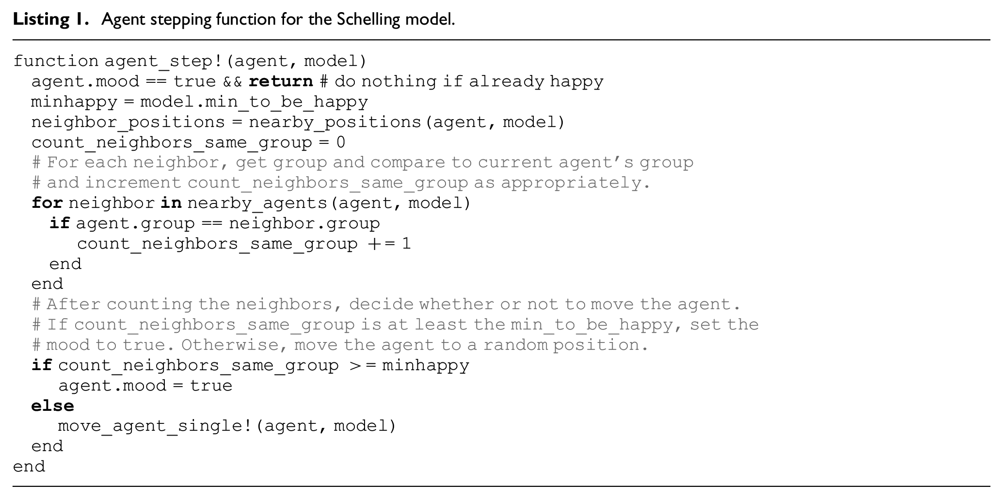
This function uses several functions from the API of Agents.jl. Specifically,
In a similar manner, one defines a model-step function. A full list of functions available from the API is described in our documentation.
2.2. Simulation run and data collection
Once the aforementioned structures and functions have been defined, the model can be evolved for one step by simply doing:
which internally takes care of scheduling agents, activating them one by one, and applying the given rules to them. The full form of step! is as follows:
where
Data collection in Agents.jl is also as simple and as general as constructing a model. This is accomplished via a two-step process. First, the user decides which data should be collected, which can be any combination of:
Agent properties;
Aggregated agent properties;
Aggregated agent properties, conditional on a user-defined filter;
Model properties.
This is done by providing vectors of appropriate entries for data collection. For example, if the user wanted to collect data for the property mood and position of the agents, they would define:
It is also possible to collect arbitrary data from an agent by providing a function, for example:
This process works identically for model parameters.
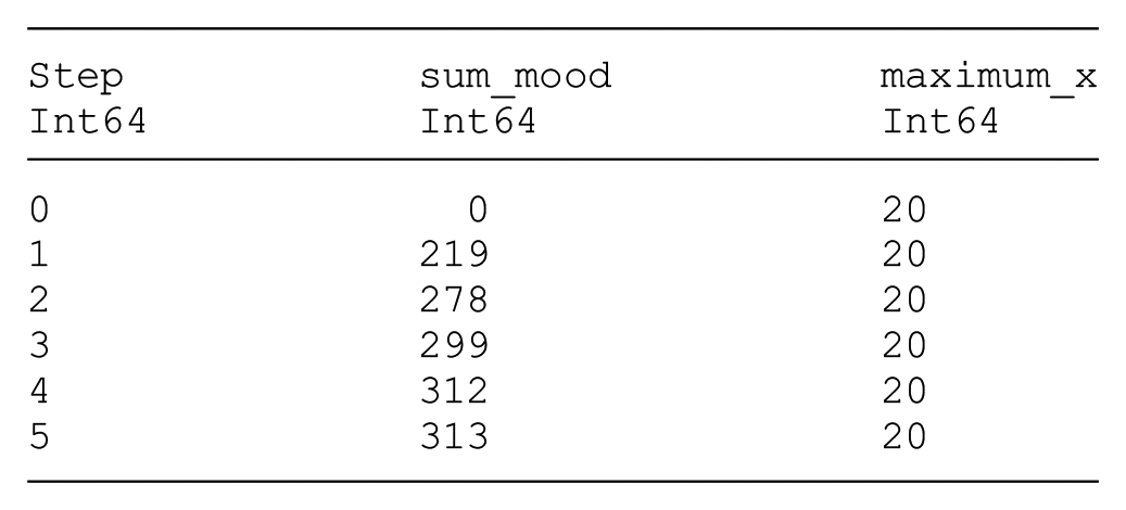
As noted above, it is also possible to aggregate agent data during data collection. For example, while getting the “mood” of each individual agent as data are sometimes desired, other scenarios may only require an aggregated result. We can achieve this by modifying the
would sum the
Once the user has defined
The
2.3. Visualization
Visualization follows the same principles as data collection. The user provides a few simple functions which decide how an agent should be represented. These user-defined functions are then given to the main plotting function
Using the current Schelling example, we can define two functions for the color and shape of the agents as follows:
The keywords
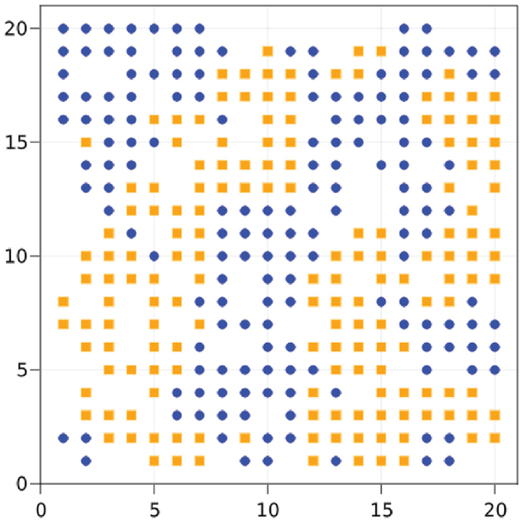
An example plot of the implementation of the Schelling segregation model in Agents.jl.
Changing
2.4. Interactive applications
By adding only a couple of lines of code (LOC) to the existing simple interface for data collection and plotting within Agents.jl, we can immediately explore an ABM in an interactive application that looks like Figure 3. The data-collection flags
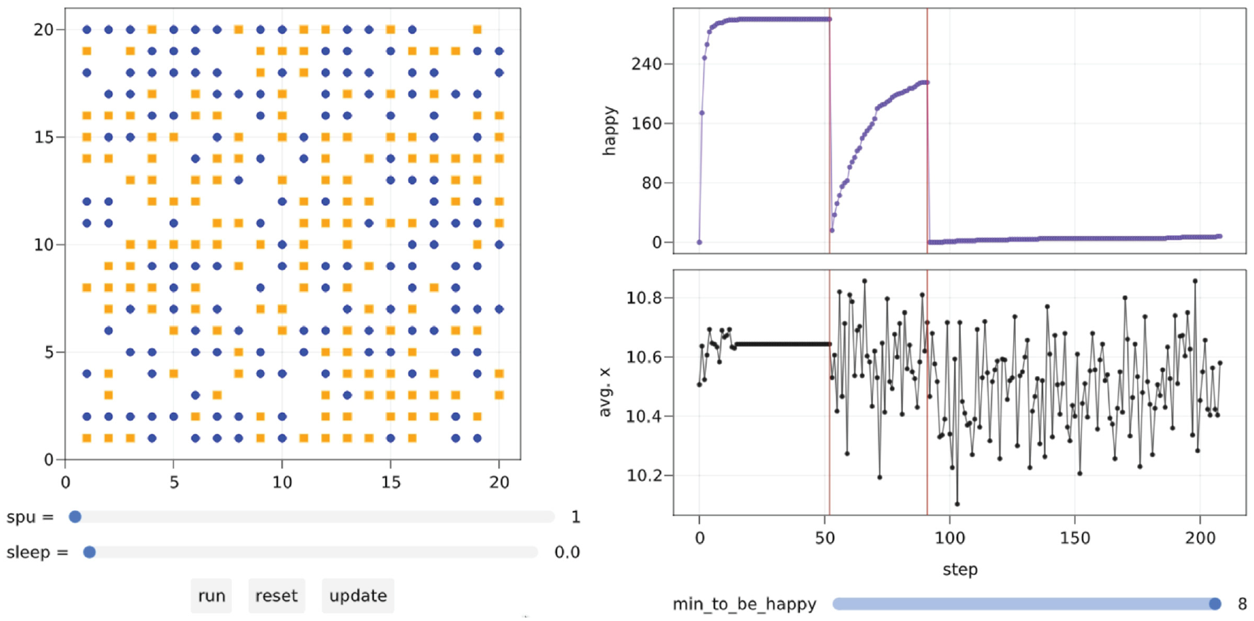
An interactive application of an agent-based model. Controls on the bottom left are created automatically and the simulation speed is tuned. Red vertical lines in the timeseries of the collected data denote when the “reset” button was pressed. Here it was pressed after the slider of the parameter “minimum to be happy” was changed from 3 to 6, and then to 8.
The only new thing the user had to define was the
3. Framework comparison
ABMs have had a long history, with many tools which enabled their construction along the way. In Table 1, we compare the software Agents.jl with three current and popular ABM software, Mesa, NetLogo, and MASON, to assess where Agents.jl excels and also may need some future improvement. This assessment is quantitative where it can be, although many aspects of the comparison are qualitative by nature. To keep the table as objective as possible, we only consider features that are directly available from the exported API of each software, and do not consider things a user could do with the software with an arbitrary amount of effort, as this is subjective and also depends on the user’s level of expertise. We categorize our results first by having either poor/none (red color), basic (yellow color), or good functionality (green color). If there is a clear category winner, this is labeled as Current Best (blue color).
Our major goal in this paper is to highlight that Agents.jl is a framework that is simple and easy to use (something hard to showcase in a comparison table, but already illustrated in the “Simulations with Agents.jl” section). Regardless, even though Agents.jl is a new-comer ABM software (development started December 2018 20 ), it becomes clear from Table 1 that we already match the main functionality of decades-old competitors (all of which are under active development), most of the time exceeding it, with only a few aspects being available in the competitors and not in Agents.jl (e.g., GIS integration).
Clarifications mapping to the superscript numbers in Table 1 are given below:
We score Dimensionalty “Current Best” for Agents.jl since it provides true N-dimensional spaces with higher-order search functions and grouping utilities. In addition, the Battle Royale example in our documentation showcases a novel application of this capability. An N-dimensional space, with a 2D spatial grid and the higher-order dimensions representing agent categories. While agent categories can be represented as standard agent properties, using additional “spatial” dimensions for them instead allows finding nearest neighbors along these dimensions, which would become cumbersome to do via the property approach.
Julia is known to provide tools for easily achieving excellent performance through parallelization. Agents.jl contains a documentation page dedicated to model performance and parallelization tips instructing users to appropriate sources. Furthermore, we provide automatic distributed computing (i.e., across multiple CPUs) for ensemble simulations or parameter scanning. Notice that in-model parallelization is outside the control of Agents.jl as it depends on the actual model operations. This stems from the nature of ABMs, where same-memory-location modifications are done all the time by killing and/or adding agents and is an active concern for all ABM frameworks.
Agent sampling is one of the many unique features of Agents.jl. It is the ability to select randomized subsets of the model population based on certain properties. Useful in biological applications, for example.
Our design of space types allows fundamentally new spaces to be created with relatively low effort. Specifically, a new space can be created by defining a new Julia struct and extending only 5 methods (i.e., defining 5 functions). The resulting space then integrates with all of the Agents.jl API as any other space would. For example, the entire implementation of our graph space is only 75 Lines Of Code (LOC).
Notice that the lack of a GUI present for simulation setup in Agents.jl is not really a lack of feature but rather a more natural consequence of the integration of Agents.jl with the entire Julia ecosystem. Julia is run in several diverse settings, from the console (REPL), to many standard IDEs like VSCode, to Jupyter and Pluto notebooks. It is also extremely straightforward to run any of these on a remote server via ssh. A GUI would not be able to run in any of these scenarios, which is in fact a downside of NetLogo and MASON (headless scripts accompany both we concede, but are considered an afterthought and have little support or flexibility). The fact that Agents.jl run in any environment that Julia can run allows it integrate in a straightforward manner into larger decision-support systems as only a sub-component of the whole process.
While the actual documentation of NetLogo is not on par with that of Agents.jl (according to our comparison), NetLogo has several associated external resources like books introducing ABMs based on NetLogo as well as educational courses. These resources however cannot be considered as part of the software (which is what we compare here), as they are not under its license. Nevertheless, they make it easier to learn.
Table 2 provides the benchmarks for four standard ABMs:
Flocking, a ContinuousSpace model, chosen over other models to include a MASON benchmark. Agents must move in accordance with social rules over the space;
Wolf Sheep Grass, a GridSpace model, which requires agents to be added, removed, and moved, as well as identify the properties of neighboring positions;
Forest Fire, which provides comparisons for cellular automata type ABMs (i.e., when agents do not move and every location in space contains a single agent);
Schelling, an additional GridSpace model to compare with MASON. Simpler rules than Wolf Sheep Grass.
The results are characterized in two ways: how long it took for each model to perform the same scenario (initial conditions, grid size, run length, etc. are the same across all frameworks), and how many LOC it took to describe each model and its dynamics. We use this result as a metric (albeit imperfect) to represent the complexity of learning and working with a framework. The time taken is presented in normalized units, measured against the runtime of Agents.jl. In other words, the results do not depend on any computers specific hardware.
For LOC, we use the following convention: code is formatted using standard practices and linting for the associated language. Documentation strings and in-line comments (residing on lines of their own) are discarded, as well as any benchmark infrastructure. NetLogo is assigned two values since its files have a code base section and an encoding of the GUI. Since many parameters live in the GUI, we must take this into account. Thus, 375 (785) in a NetLogo count means 375 lines in the code section, a total of 785 lines in the file. An additional complication to this value in NetLogo is that it stores plotting information (colors, shapes, and sizes) as agent properties, and as such the number outside of the bracket may be slightly inflated.
Analyzing the performance between the frameworks was difficult, since each system implements example models in their own unique manner. This highlights the lack of standardized bench-marking models, perhaps stemming from the lack of communication between the ABM communities. Since the Wolf-Sheep-Grass model requires frameworks to utilize most of the common machinery (multiple agent types, adding, deleting, and moving agents), we would appreciate if the MASON community (and ABM communities as a whole) could provide an implementation of this model for future comparisons. From the analysis we present here, Agents.jl is a clear winner in performance, most of the time by an order of magnitude. Since typical ABM simulations can cover hours of run time, even a 2× speed up is a large gain.
JuliaDynamics hosts the ABM Framework Comparisons repository 21 for anyone who wishes to validate these results, improve implementations, or add new comparisons.
4. Ecosystem interaction examples
In this section, we want to showcase how easily Agents.jl interacts with the rest of the Julia ecosystem. This is possible for two reasons: first, the minimal design of Agents.jl, as well as the support it provides for low-level interfaces. Second, the design of the core of the Julia language itself, which allows straightforward inter-package communication. Note that the examples we showcase here have fully detailed documentation online, explaining precisely how they work. Our goal here is to highlight how easy it is for Agents.jl to “communicate” with other Julia packages, removing any need for a plugin or extension ecosystem and thus making the user experience smoother.
4.1. Ordinary differential equations with DifferentialEquations.jl
Coupling a set of differential equations (DEs) to an ABM has historically led to a complex set of validation and sensitivity tests, 22 which stem from discretizing a DE in some manner (predominantly via the forward Euler method) to conform with the step function of the ABM framework. The tests outlined in Martin and Schlüter 22 concerning sensitivity can be handled automatically by integrating Agents.jl with DifferentialEquations.jl. 23
To demonstrate this, our documentation (under the “Ecosystem Integration” section) describes a small fishery model where fish stocks are managed on a yearly basis. A number of fishers, with differing competence at catching fish, work in a common catchment. This is managed by some agency that makes sure the catchment is not over-fished. The fish population in the catchment is modeled via a logistic function:
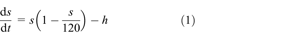
where
The status-quo method to implement such a hybrid dynamical system, ABM, is to discretize this equation to:

with a timestep of 1 normalized unit initially. To validate this result, it would be important to undertake a step size analysis as a bare minimum, and to be thorough, use a scheme such as the one outlined in Martin and Schlüter. 22 Thankfully, the issues caused by discretization do not need to exist within an Agents.jl model, as we can couple our model with a continuous implementation of the DE from DifferentialEquations.jl.
We can see from Figure 4 that a forward Euler method with no step size optimization performed (or further sensitivity checks as discussed above) will yield an average discrepancy of 30 fish. Integration with DifferentialEquations.jl has provided us with a stable, valid solution—with an added bonus of efficiency. Since the chosen solver (in this case,
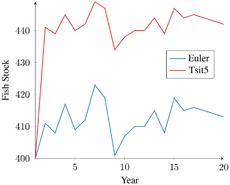
Comparative result of a continuous DE solution
4.2. Agents on Open Street Maps
With our new space type API, building ABMs on novel spaces is no longer a months-long development process. An
Our Zombie Outbreak example (see documentation online) explains how a simple agent constructor:
coupled with 8 lines of movement dynamics can depict a city in chaos after a zombie infection (Figure 5).
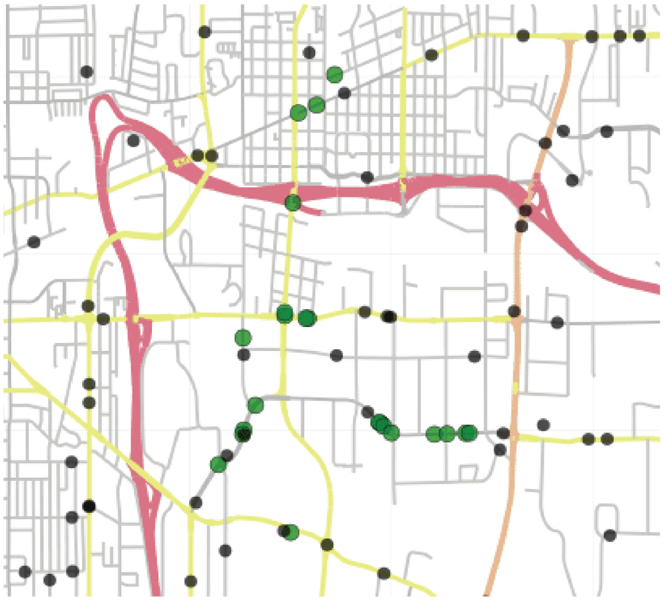
Agents following planned routes on a map, interacting with passers-by. Black markers: agents, green markers: zombies!
4.3. Parameter optimization
Describing the logic of an ABM is usually not complicated, even when ABMs have a large number of heterogeneous agents. 24 However, exploring the effect of model parameters has the possibility to become infeasible. ABMs are often computationally more expensive than analytical models, and brute force algorithms do not suit parameter exploration since the size of the parameter space of a simple model with 10 parameters and 10 possible values per parameter is 1010. Even if each simulation takes only 1 s, exploring the entire parameter space would take more than 300 years. In addition, each parameter setting needs to be run multiple times and an average taken, since most ABMs are stochastic. Machine learning algorithms handle the large parameter space by differentiation. ABMs, however, are not (universally) differentiable.
We must resort to optimization strategies for non-differentiable functions. One such strategy is evolutionary algorithms. 25 They are inspired from how living organisms evolve in a constantly changing environment and with large parameter spaces, similar to how ABMs often need to explore large parameter spaces.
The Agents.jl documentation demonstrates how an epidemiological model can be optimized with evolutionary algorithms using the BlackBoxOptim.jl package. We optimize a number of parameters of a SIR model (SIR stands for Susceptible-Infected-Recovered and is a simple model for infection dynamics commonly used in ABMs) explicitly accounting for multiple cities/regions. Specifically, we tune the transmission rate, death rate, migration rate, infection and detection times, and reinfection probability to minimize the number of infections. We note that to optimize the ABM, the simulation code does not need to be changed. All we need is a cost function that takes model parameters as input, runs the model one or more times, and returns one or more numbers as the objectives that need to be minimized (here, the number of infected individuals and the negative of the number of individuals). With our initial values, 94% of the population gets the infection. The optimization finds that reducing the transmission rate is enough for reducing the death rate and infections to 0.3% and 0.04% of the population, respectively, despite increasing the reinfection probability, migration rate, and death rate. Accessibility of optimization tools in the Julia ecosystem and their easy integration with Agents.jl make ABM analysis much easier.
5. Conclusion and future work
We have presented an overview of the capabilities of Agents.jl, showing the simplicity and power of this framework compared to long-established frameworks (e.g., NetLogo and MASON), as well as contemporaries (Mesa). From our perspective, the biggest take-away of this paper is that Agents.jl is a framework that is simple to use, requiring small amount of written code from the user, and overall easy to learn. Despite this, our comparison shows that Agents.jl always exceeds other frameworks in performance, and often also in capability. An added bonus is how simple it is for a user to incorporate other parts of the already large, and constantly evolving, Julia ecosystem into their model. With this, we hope to motivate more users to try out Agents.jl, which will enable them to extend the frontier of possibilities in the world of ABMs, due to faster prototyping and faster code execution.
Several possible future directions already exist for Agents.jl, some planned by the developers and others requested by users. A useful new feature would be crowd dynamics and obstacle avoidance, as well as a new type of grid space based on hexagonal grids, rather than the existing rectangular. The ODD (Overview, Design concepts, Details) protocol 26 is a formal description of ABMs, aiming to make models more understandable and less subject to criticism for being irreproducible. While Agents.jl models are reproducible by design, a planned feature will leverage Julia’s strong macro language capability to pre-fill many aspects of the standard ODD template. Integration into the greater Julia ecosystem is useful to highlight as well: one upcoming integration will target Bayesian inference for decision making. A performance issue Agents.jl currently has is regarding multi-agent models (even though, it is still the fastest software in this regard). In the future, we plan to re-work our multi-agent internals from scratch to lead to more performant, but not more complicated, designs.
Given that Agents.jl is an open-source project, we welcome new users to add to the wish-list of functionalities by opening a new issue in our GitHub repository, or even better, to contribute new features via a pull request.
Footnotes
Acknowledgements
The authors acknowledge all users of Agents.jl who contributed in the form of reporting bugs, suggesting new features, and even contributing code directly via pull requests.
Author contributions
G.D. provided direction to the team, refactored and optimized much of the current codebase, oversaw critical design decisions regarding the representation of spaces and plotting, and served as lead developer from v2.0 until v4.0. A.R.V. is the original author of Agents.jl and has been continuously active in development since. T.C.D. is the current lead developer of Agents.jl, has been active in development since version v2.0, implementing and optimizing a large portion of the framework and contributing several new features and examples. A.R.V. drafted the introduction section, and G.D. drafted the usage section and the outline of the comparison table. Mesa comparisons were compiled by A.R.V., all other frameworks by T.C.D. Benchmarks were run and listed by T.C.D. T.C.D. and A.R.V. wrote the Ecosystem Integration. All the authors contributed to draft revisions and editing.
Funding
The author(s) disclosed receipt of the following financial support for the research, authorship, and/or publication of this article: T.C.D. acknowledges funding from the EU project LimnoScenES (2017–2018 Belmont Forum and BiodivERsA joint call under the BiodivScen ERA-Net COFUND with funding from the Swedish Research Council FORMAS).