A novelty mode decomposition method and its application in dynamic characteristic identification of bridge GNSS monitoring data

Abstract

As the majority of real signals (e.g., the dynamic information obtained during bridge Global Navigation Satellite System (GNSS) monitoring) are nonlinear and nonstationary, variational mode decomposition (VMD) and its derivatives have become popular research topics in recent years worldwide. However, the VMD method has the problem in which improper parameter selection results in a poor decomposition effect. This study analyzes the different decomposition effects of the VMD parameters, such as the decomposition layer number K, the modal frequency bandwidth control parameter $\alpha$ and the noise tolerance $\tau$ , and ascertain the insufficiency of the existing optimization methods. On the basis of the investigation and analyses of several decomposition effect evaluation indicators, an adaptive variational modal decomposition algorithm based on multi-objective particle swarm optimization (AVMDbMOPSO) is proposed. The results of our experimental analysis indicate that the method can effectively extract multi-frequencies. Advantages emerge with regard to practical signals collected via the GNSS monitoring of the dynamic characteristics of a bridge. The findings of this research have a positive significance for practical engineering applications.

1. Introduction

Similar to other building structures, the modal parameters of a bridge—including natural frequency, mode shape, and modal damping—are functions of its physical properties such as mass, damping, and stiffness. Consequently, any changes in these physical characteristics result in corresponding changes in the modal parameters.^1,2 In other words, environmental factors like loading conditions, ship collisions, and material aging can excite the bridge structure and induce dynamic responses. ² Early detection of abnormal deformations or frequency shifts, along with timely interventions before structural damage accumulates to a critical level, can help prevent severe casualties and economic losses. ³ Following consistency checks between GNSS-based displacement monitoring and total station measurements,^4,5 as well as between GNSS-derived frequencies and accelerometer data,^6,7 growing attention has been paid by researchers and engineers to GNSS-based techniques for structural monitoring. These include advanced GNSS positioning methods, high-sampling-rate GNSS receivers,^8,9 multi-frequency and multi-system GNSS configurations, multipath effect mitigation, ¹⁰ noise characterization, ¹¹ and signal denoising techniques. These continuous improvements enable the extraction of continuous, real-time, high-frequency micro-deformation data from major engineering structures. As a result, GNSS dynamic monitoring data are becoming an increasingly vital reference for assessing the safety status of bridge structures.^12,13 Deformation monitoring primarily focuses on both static and dynamic behavior, including position, displacement, settlement, and linear or even nonlinear deformations of structural components. Among the modal parameters, the natural frequency (or terms as vibration frequency) is the most readily accessible. ¹⁴ Unlike accelerometers, which lack a trend term and require integration that may introduce errors, ¹⁵ the natural frequency extracted from long-term high-frequency monitoring time series serves as a key indicator of structural safety.^13,16–22

However, GNSS dynamic monitoring data of bridges are influenced by traffic loads and environmental excitations, resulting in highly complex nonlinear and nonstationary signal characteristics. Due to multipath effects and random errors, the true dynamic displacements are often obscured by strong noise, limiting the applicability of GNSS for modal identification. Therefore, effective data preprocessing is essential to mitigate measurement errors before extracting structural dynamic features. ²³ Moreover, identification methods should be advanced based on the time–frequency characteristics of GNSS data, particularly to capture subtle frequency variations in bridge structures. ²⁴

To date, researchers have employed a variety of techniques to extract vibration modal parameters from nonlinear and nonstationary GNSS monitoring data. These include Fourier transform,^24,25 wavelet analysis,^26–29 empirical mode decomposition (EMD),^30–32 and ensemble empirical mode decomposition (EEMD).^33–37 For instance, Huang and Wang et al. ¹⁶ introduced a hybrid method combining EMD, permutation entropy (PE), and spectral substitution to suppress noise while preserving signal content. This approach, applied to noisy GNSS data from the Wuhan Baishazhou Yangtze River Bridge—referred to as PSEEMD—yielded significantly clearer dynamic characteristics. Wang et al. ³⁸ proposed a time–frequency method integrating wavelet threshold denoising with Hilbert–Huang Transform (HHT), which accurately reflected the spectral properties of the bridge and aligned well with theoretical predictions. In another study, Wang et al. ¹⁸ developed an adaptive stochastic resonance method based on a quantum genetic algorithm to extract reliable dynamic features from GNSS signals. While these methods have shown some success, they still face limitations in effectively handling frequency variations, especially in the context of nonlinear and nonstationary signal transitions.

Variational mode decomposition (VMD), introduced by Dragomiretskiy et al. ³⁹ in 2014, offers a novel approach to signal processing. VMD identifies the frequency center of each component through iterative optimization of a variational model. It simultaneously determines the center frequency and bandwidth for each mode, enabling effective frequency-domain separation and component isolation. ³⁸ Unlike EMD, which recursively decomposes signals, VMD simultaneously extracts all modes by estimating band-limited intrinsic mode functions and adaptively determining their center frequencies. ³⁹ Experimental results from Dragomiretskiy et al. ³⁹ demonstrated the superiority of VMD over EMD in tone detection, signal separation, and noise robustness, a conclusion further supported by Wang and Markert. ⁴⁰ Consequently, VMD has been widely adopted in mechanical fault diagnosis.^41–46 In civil engineering, Zhang et al. ⁴⁷ applied VMD to modal identification and confirmed its advantage over EMD in decomposing certain types of vibration signals.

Therefore, the selection of the right parameters for combination is a primary problem in signal decomposition for the VMD method and thus has become the focus of research by many scholars. Li et al. ⁴⁶ proposed a VMD parameter optimization method based on independence but did not consider the impact of the penalty coefficient on the decomposition result. Shi and Yang ⁴⁸ proposed a method to optimize VMD, but the interaction between two parameters was ignored, and the algorithm tended to fall into local optimization. Yan et al. ⁴⁹ proposed a genetic algorithm-based optimization VMD method to optimize two parameters at the same time. However, the optimization objective function (envelope spectrum entropy value) employed only considered the influence of the decomposition mode characteristics, but the correlation between the inherent modal components and the original signal were ignored. In such scenarios, information loss may occur. As the VMD parameter optimization objective function directly affects the accuracy and efficiency of the final decomposition, this problem is worthy of attention and requires urgent investigation.^50,51

The objective of this project is related to modal identification and analysis. By improving the method of VMD parameter optimization based on multi-objective particle swarm optimization (MOPSO), the optimized VMD parameters can provide the dynamic characteristics needed to assess the health condition of operational bridges (as shown in Figure 1). The paper is arranged as follows. Section 2 provides a general description of VMD and its superiority as a method. Section 3 is devoted to the review of previous works that include topics on how the VMD parameters influence the effect of decomposition and the shortcomings of existing parameter optimization methods. The parameter-optimized VMD method based on the MOPSO algorithm is investigated in Section 4. Section 5 provides the simulation experiment and example verification. Section 6 and 7 gives discussions and the concluding remarks. The technical route of this study is shown in Figure 1.

Figure 1.

The technical route of this study.

2. VMD and its superiority as a method

2.1. The VMD method

Different from the intrinsic mode function (IMF) defined by EMD that must meet strict conditions, VMD defines IMF as an amplitude modulation–frequency modulation signal according to the formula

$u_k\left(t\right)=A_k\hspace{0.17em}\cos \left({\psi }_k\left(t\right)\right)$

(1)

where $A_k\left(t\right)$ is the instantaneous amplitude of $u_k\left(t\right)$ , and ${\omega }_k\left(t\right)$ is the instantaneous frequency of $u_k\left(t\right)$ , such that $\omega \left(t\right)={\psi }_k^{\prime }\left(t\right)=\frac{d{\psi }_k\left(t\right)}{dt}$ . Compared with the phase ${\psi }_k\left(t\right)$ , $A_k\left(t\right)$ is used, and it changes relatively slowly. In other words, in the smaller interval $\left[t-\delta ,t+\delta \right]$ ( $\delta =2\pi /{\psi }^{\prime }\left(t\right)$ ), $u_k\left(t\right)$ can be regarded as a cosine signal with the amplitude $A_k\left(t\right)$ and frequency ${\omega }_k\left(t\right)$ ³⁹ .

Similarly, different from the processing method and derivative algorithms of signal stripping by means of empirical screening in EMD, VMD transfers the signal decomposition process to the variational framework and searches for the optimal solution of the constrained variational model to achieve decomposition. ³⁹

Each frequency center and bandwidth of the IMF component of VMD (to distinguish between the IMF obtained by EMD and its derivative algorithms, the IMF of the VMD method here is abbreviated as VIMF, and the same applies hereafter) are continuously updated under the action of related parameters in the process of iteratively solving the variational model. Then, the frequency domains reflecting the characteristics of the signal may be subdivided automatically, and the several specified VIMF components can be obtained. ³⁹

If a certain nonlinear and nonstationary signal $f_{-}s$ can be decomposed into K VIMF components, the corresponding constrained variational model can be represented as

$\begin{array}{c}\underset{\left\{u_k\right\}\to \left\{{\omega }_k\right\}}{\min }\left\{{\displaystyle \sum }_k{\Vert {\partial }_t\left[\left(\sigma \left(t\right)+\frac{j}{\pi t}\right)u_k\left(t\right)\right]e^{-j{\omega }_{k}t}\Vert }_2^2\right\}\\ s.t{\displaystyle \sum }_k{u}_k=f_{-}s\end{array}\}$

(2)

where $\left\{u_k\right\}=\left\{u_1,u_2,\cdots ,u_k\right\}$ is the K VIMF components derived via the decomposition, and $\left\{{\omega }_k\right\}=\left\{{\omega }_1,{\omega }_2,\cdots ,{\omega }_k\right\}$ is the frequency center of each component. ³⁹

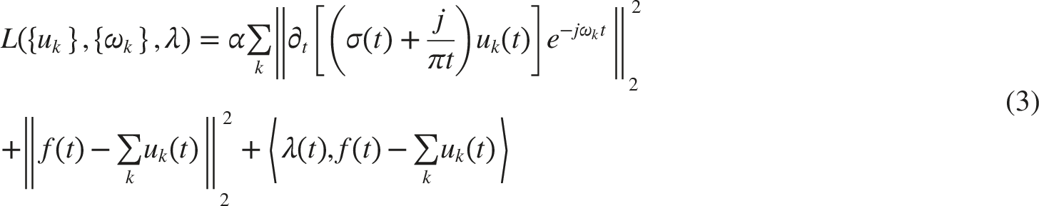
In solving the optimal solution of Equation (2), an augmented Lagrange function is constructed as follows:

$\begin{array}{l}L\left(\left\{u_k\right\},\left\{{\omega }_k\right\},\lambda \right)=\alpha {\displaystyle \sum }_k{\Vert {\partial }_t\left[\left(\sigma \left(t\right)+\frac{j}{\pi t}\right)u_k\left(t\right)\right]e^{-j{\omega }_{k}t}\Vert }_2^2\\ +{\Vert f\left(t\right)-{\displaystyle \sum }_k{u}_k\left(t\right)\Vert }_2^2+〈\lambda \left(t\right),f\left(t\right)-{\displaystyle \sum }_k{u}_k\left(t\right)〉\end{array}$

(3)

where $\alpha$ is the penalty factor, and $\lambda$ is the Lagrange multiplier.

The approach called alternating direction method of multipliers (ADMM) is commonly employed to solve the saddle point of the augmented Lagrange function of Equation (3), and then the optimal solution of the constrained variational model is obtained. That is, ADMM is used to decompose the original nonlinear and nonstationary signal into K narrowband VIMF components. ³⁹

2.2. Implementation steps of VMD

The implementation steps of the VMD algorithm ³⁹ are as follows:

(1) Initialize $\left\{u_1\right\}$ , $\left\{{\omega }_1\right\}$ and ${\lambda }_1$ , and $n=0$ ;

(2) Assign a new value to the loop $n=n+1$ , and execute the loop;

(3) Implement the first cycle of the inner layer, and then update $u_k$ according to $u_k^{n+1}\leftarrow \underset{u_k}{\mathrm{argmin}}\left[L\left(\left\{u_{i<k}^{n+1}\right\},\left\{u_{i\ge k}^n\right\},\left\{{\omega }_i^n\right\},{\lambda }^n\right)\right]$ ;

(4) Update the number of iterations with $k=k+1$ . Repeat step (3) until $k=K$ , and let the first loop of the inner layer end;

(5) Implement the second cycle of the inner layer. Update ${\omega }_k$ according to ${\omega }_k^{n+1}\leftarrow \underset{{\omega }_k}{\mathrm{argmin}}\left[L\left(\left\{u_i^{n+1}\right\},\left\{{\omega }_{i<k}^{n+1}\right\},\left\{{\omega }_{i\ge k}^n\right\},{\lambda }^n\right)\right]$ ;

(6) Update the number of iterations with $k=k+1$ . Repeat step (5) until $k=K$ , and let the second loop of the inner layer end;

(7) Update ${\lambda }^n$ according to ${\lambda }^{n+1}={\lambda }^n+\tau \left(f_{-}s-{\displaystyle \sum }_k{u_k}^{n+1}\right)$ ;

(8) Repeat steps (2) to (7) until the iteration stop condition ${\displaystyle \sum }_k\left({\Vert u_k^{n+1}-u_k^n\Vert }_2^2/{\Vert u_k^n\Vert }_2^2\right)<\epsilon$ is satisfied. Then, let the entire loop end. The decomposition structure is outputted, and the K narrowband VIMF components are obtained.

The VMD algorithm needs to specify the following four parameters in advance ⁵² : number of modal layers K, modal frequency bandwidth control parameter (or quadratic penalty term) $\alpha$ , noise tolerance $\tau$ , and convergence criterion tolerance $\epsilon$ .

2.3. Superiority analysis of VMD

A simulation-combined signal composed of three sinusoidal signals and noise is constructed to verify the differences in the decomposition effects of VMD, EMD and the derivative algorithms.

$s_1=\sin \left(2\pi ·15·t\right).,s_2=\frac{1}{3}\sin \left(2\pi ·40·t\right)$

(4)

$s_3=\left(1/5\right)\sin \left(2\pi ·200·t\right),s=s_1+s_2+s_3$

(5)

$S_6=s+noise6$

(6)

where $noise6$ is a Gaussian white noise sequence with a mean value of 0 and a variance of 1. The sampling interval is 1000, and the data length is 4000. The simulation signal $S_6$ and the waveforms of each component are shown in Figure 2. The amplitudes of the different components of the simulated signal clearly depict a wide difference.

Figure 2.

Time domain waveform of the combined signal $S_6$ .

The nonlinear and nonstationary signal is processed by the EMD method. The diagram of the time–frequency analysis is shown in Figure 2. Due to the modal aliasing, the first three components seem to all contain the frequency component of $s_3$ , which corresponds to the third component shown in Figure 2. However, the whole signal is interfered seriously by noise. The fifth and sixth IMF components in Figure 3 correspond to the $s_2$ and $s_1$ components in Figure 2, respectively. A certain noise interference is also apparent. In addition, due to the characteristics of the EMD algorithm itself, some components without actual physical meanings are produced as shown by the last several components in Figure 3.

Figure 3.

Time domain of IMF components of the simulation signal $S_6$ processed by EMD.

The simulation signal is processed by the PSEEMD method by using the same parametric settings, which is similar to that in Ref. ¹⁸ , and the time–frequency analysis diagram is shown in Figure 4. Similar to the EMD method, PSEEMD obtains the first three components containing the $s_3$ frequency components due to modal aliasing. However, although PSEEMD does not produce too many meaningless IMF components, and the component $s_2$ is separated, the $s_1$ component cannot be decomposed successfully because this method requires an obvious extreme value after fast Fourier transform (FFT) processing. This scenario indicates that PSEEMD cannot effectively decompose mixed noisy signals with great amplitude disparity.

Figure 4.

Time domain of IMF components of the simulation signal $S_6$ processed by PSEEMD.

The VMD mode layer number is K = 4, the penalty factor is $\alpha =10000$ , the error tolerance is $\tau =0.004$ , and the convergence criterion tolerance is $\epsilon ={10}^{-7}$ . Then, the simulation signal is processed by the VMD method, as described in Section 2.2. The diagram of the time–frequency analysis is shown in Figure 5. The VMD method can clearly decompose the three sinusoidal signal components of the original signal and arrange them from the low to high frequencies. The first and second VIMF components are consistent with the 15 and 40 Hz components, and the frequency spectrum is relatively clean and without noise. The third VIMF component contains a certain amplitude of noise, but the 200 Hz components appear to be clear. The fourth VIMF component is the separated noise. Overall, there are no other components exist. Hence, the VMD method can avoid the shortcomings of EMD and its derivative algorithms that produce components without actual physical meanings.

Figure 5.

Time domain of VIMF components of the simulation signal $S_6$ processed by VMD.

The combination and analyses of the frequency spectra of the (V)IMF component obtained by the aforementioned three methods further suggest that VMD not only can avoid modal aliasing effect but also has a good denoising effect.

3. Functions of VMD parameters and existing parameter optimization methods

As mentioned previously, the VMD algorithm comprises the following four parameters: K, $\alpha$ , $\tau$ , and $\epsilon$ . For the simulation signal or the actual signal with known characteristic parameters, which are detected on the basis of experience, each parameter value can be set in advance for VMD analysis. Decomposing the signal with specified parameters is a suitable approach and comparable to that in Section 2.3 owing to the good frequency extraction and denoising effect. As the majority of the real signals (e.g., dynamic information obtained during bridge monitoring) are nonlinear and nonstationary, their characteristic parameters are unknown until they are monitored or studied. On the basis of investigation and understanding of the parameters’ characteristics in the VMD method, many researchers have widely investigated the different VMD parameter optimization methods. ⁵² However, the different methods have their own certain shortcomings. In this section, the influence of the different parameters on the decomposition effect of VMD is discussed and analyzed to fully understand the parameter optimization method.

3.1. Influence of different parameters on the decomposition effect of VMD

Determining the best parameters that match the signal to be analyzed is necessary in understanding the impact of each parameter on the decomposition effect of the VMD algorithm. A possible approach is to consider one of the important ways for obtaining human knowledge—comparative observation method. In this scheme, each influential parameter changes constantly, whereas the other influencing parameters remain constant. Then, their influences on the VMD decomposition effects are sequentially explored. On the basis of the aforementioned purpose, the simulation signal consisting of the frequency modulation, sinusoidal, intermittent sinusoidal, and noise signals is constructed as follows:

$s_1=\left[0.5+0.8·\sin \left(2\pi ·5·t\right)\right]·\sin \left(2\pi ·40·t\right)$

(7)

$s_2=\{\begin{array}{ll}0.8·\sin \left(2\pi ·120·t\right),& t\le 0.75·N\\ 1.2·\sin \left(2\pi ·90·t\right),& t>0.75·N\end{array}$

(8)

$s_3=\sin \left(2\pi ·190·t\right)+1.2·\sin \left(2\pi ·220·t\right)$

(9)

$s=s_1+s_2+s_3,S_7=s+\mu ·noise7$

(10)

where $noise7$ is a Gaussian white noise sequence with a mean value of 0, a variance of 1, and a sampling point of 4000. The other parameters are set in the same manner with $S_6$ as those in Section 2.3. The waveform of the simulation signal $S_7$ ( $\mu$ is set to 2). The respective components are shown in Figure 6.

Figure 6.

Time domain waveform of the combined signal $S_7$ .

A nonlinear and nonstationary signal ( $S_7$ ) clearly contains five different types of pure signal components (to facilitate the problem, $s_2$ and $s_3$ in Equation (10) are separated as $sc2$ , $sc3$ , $sc4$ and $sc5$ corresponding to the third, fourth, fifth and sixth subfigures in Figure 6). The noise-added waveform of $S_7$ is shown as the first subfigure. $sc2$ and $sc3$ are segmented intermittent signals with different magnitudes, hence the variations in the modal decomposition of the respective frequency domain. The main frequencies may be difficult to extract or identify by EMD and its derivative algorithm due to the effect of noise. Furthermore, the frequencies between $sc2$ and $sc3$ and between $sc4$ and $sc5$ are all small. Thus, the EMD and its derivative algorithm may have generated the modal aliasing in the signal decomposition. These simulation signals are similar to the case of the bridge coordinate time series data monitored by the GNSS.

3.1.1. Influence of parameter K

In the investigation of the influence of parameter K on the VMD decomposition effect, the parameters are set as $\alpha =4000$ and $\tau =0.0005$ , and K is set from 3 to 15. The multi-component frequency modulation signal $S_7$ is decomposed by the VMD method. Due to the limited space of this paper, only the part regarding the decomposition effect is shown as diagrams in Figure 7.

Figure 7.

Decomposition effect of VMD with different K values.

As shown in Figure 7(a), VIMF1 corresponds to the $sc1$ component in Figure 6 when K = 4, which could be considered that the frequency modulation signal is correctly separated. However, there are insufficient decomposition of signal $S_7$ by VMD, and there are serious modal aliasing in the obtained VIMF components. For example, VIMF2 here corresponds to the $sc2$ and $sc3$ components in Figure 6, and the corresponding $sc3$ component is so weak that it is almost unrecognizable. Similarly, the component VIMF3 corresponding to the $sc4$ and $sc5$ components in Figure 6, also there are also modal aliasing, and the corresponding component $sc4$ is also weak. The VIMF4 component can be considered as a noise component.

There are also insufficient decomposition of signal $S_7$ by VMD when K= 3, 5 and 6, and there are also modal aliasing in the obtained VIMF components (These figures are omitted to save space). It is important to note as well that even if the VMD decomposition layers of signal $S_7$ is set to 6 in theory as shown in Figure 6 (the number of signal components of $S_7$ is 5, and that plus the noise term), the VMD decomposition results at this time are still not match the true situation. As shown in the decomposition result of K = 7 (Figure 7 (b)), the component VIMF4, corresponding to the component $sc4$ and $sc5$ in Figure 6, also has a modal aliasing phenomenon, and VIMF5, VIMF6, VIMF7 are considered as noise components. These are also inconsistent with the actual situation.

When it comes to K = 8, the VMD processed result is shown in Figure 7(c). It can be inferred that the components VIMF1-VIMF5 are in good agreement with the $sc1$ - $sc5$ components in Figure 6, even though 3 noise component terms VIMF6-VIMF8 are also generated. This means that the proper number of VMD decomposition layers that may obtain a better decomposition effect may be more than 1 more than the actual number of components of the composite signal. Of course, it should also be seen that although the noise component items in the VMD decomposition result at K = 8 are all high-frequency in the frequency domain, their amplitudes are all small.

When the parameter K continues to increase to 9, the first 5 components via VMD processing are also in good agreement with the components of signal $S_7$ as shown in Figure 7(d). The number of their noise items increases just by 1, and these noise items are also at high frequencies with small amplitudes. Therefore, it cannot be judged intuitively from the figures which value of 8 or 9 for K the VMD algorithm may obtain better decomposition effect. Therefore, it is believed tentatively that in this case, the decomposition layer number K of 8 or 9 can achieve a satisfactory decomposition effect.

When the parameter K increases further to 10, the VIMF2-VIMF9 components of the obtained decomposition result (Figure 7(e)) share a high similarity as those of the components in Figure 6. However, an emerging component (VIMF1), which does not match any component of the original signal, can be observed. As such, this component can be judged as a noise term or a meaningless component. As the VIMF2–VIMF9 components in the results are in good agreement with those of the original signal, and the noise items can be distinguished and eliminated, the decomposition effects are likely acceptable when K = 10. However, this finding also indicates that the signal is overly decomposed when the parameter K of VMD increases to 10.

When the parameter K increases gradually to 11, 12, 13, 14, and 15, a phenomenon of excessive decomposition is observed, which is in good agreement with some VIMF components in the VMD result and the corresponding components of the original signal. Only the VMD decomposition result of K = 15 is plotted in Figure 7(f) to save space in this paper, and “vi” is used instead of “vimfi” ( $i=3,4,\cdots ,15$ ) to clearly express the components of the multiple VMD decomposition results. It can be inferred from the figure that the noise items VIMF1 exists at the beginning, VIMF9–VIMF15 at the end part, and VIMF3 and VIMF7 in the middle part. As such, the decomposition phenomenon is seriously excessive in the result of the VMD decomposition when the parameter K is increased to a certain extent.

The aforementioned analysis indicates that the setting of K is particularly important to the decomposition effect of the VMD algorithm. A suitable K value is needed to properly and effectively decompose the nonlinear and nonstationary signal. By contrast, insufficient or excessive decompositions of the original signal may occur for the smaller or larger K values.

3.1.2. Influence of parameter $\alpha$

In investigating the influence of parameter $\alpha$ on the VMD decomposition effect, the parameters are set as $K=8$ , and $\tau =0.0005$ . The parameter $\alpha$ is set from 200 to 10000, varies each time by 200. The multi-component frequency modulation signal $S_7$ is decomposed using the VMD method. However, given the limited space in this paper, only the part of the decomposition effect is shown in the diagrams in Figure 8(a)–(f).

Figure 8.

Decomposition effect of VMD with different $\alpha$ values.

As shown in Figure 8(a), VIMF1 corresponds to the $sc1$ component in Figure 6, VIMF3 corresponds to $sc4$ , and VIMF4 corresponds to $sc5$ when $\alpha$ =200, suggesting that these frequency components of the signal are correctly separated. However, a serious modal aliasing can be observed in the obtained VIMF components when VMD is used. Here, VIMF2 corresponds to the $sc2$ and $sc3$ components in Figure 6. The corresponding $sc3$ component is extremely weak as it is almost unrecognizable. The subsequent VIMF5, VIMF6, VIMF7, and VIMF8 components are likely noise items whose amplitudes are not high and whose main frequency bands increase sequentially. Therefore, when $\alpha$ =200, the VMD algorithm may have incorrectly decomposed all of the components of the combined signal $S_7$ . The decomposition phenomenon is insufficient in the result of the VMD decomposition even when $\alpha$ is set as large as to 400 (limited by space, the renderings are not listed in this paper).

The parameter $\alpha$ is then increased to 600. The VMD-processed result is shown in Figure 8(b). The components VIMF1–VIMF5 here are in good agreement with the $sc1$ - $sc5$ components in Figure 6. However, the three noise component terms VIMF6–VIMF8 are also generated. Although the noise component items in the VMD decomposition result for $\alpha$ = 600 are all high-frequency components in the frequency domain, their amplitudes are all small.

When the parameter $\alpha$ continues to increase, the first five components via VMD processing are also in good agreement with the components of signal $S_7$ . The respective VMD-processed results when the parameter $\alpha$ increases to 1000 and 7400 are shown in Figure 8(c) and (d). Even if the parameter $\alpha$ changes from 600 to 1000 and finally to 7400, judging intuitively from the figures which parameter value causes the VMD method to obtain a better decomposition effect is difficult based on experimental analysis. Given this finding, many VMD decomposition renderings with the parameter $\alpha$ varying from 800 to 7200 are not presented in the text. In this case, it can be tentatively assumed that the VMD method can achieve a satisfactory decomposition effect when the parameter $\alpha$ varies from 800 to 7200. The respective VMD-processed results when the parameter $\alpha$ increases further to 7600 are shown in Figure 8(e). Here, VIMF2 corresponds to the $sc1$ component in Figure 6, VIMF3 corresponds to $sc3$ , and VIMF4 corresponds to $sc4$ , suggesting that parts of the frequency component are correctly separated when $\alpha$ = 7600. However, determining the corresponding component from Figure 6 that is equivalent to the component VIMF1 in the VMD-processed results is difficult. Furthermore, the corresponding approximate shape of the $sc2$ component from Figure 6 cannot be easily identified. Even if the decomposition results of the three noise component terms VIMF6, VIMF7, and VIMF8 here are equivalent to that of the VMD-processed results at $\alpha$ =7400, the decomposition effect is clearly poor at this time. Similarly, even if the parameter $\alpha$ increases from 7800 to 10000, the decomposition effect is still weaker than that shown in Figure 8(e). As shown in Figure 8(f), the incorrect value of parameter $\alpha$ can affect the correctness of the decomposition results.

In summary, an appropriate value of the parameter $\alpha$ is required to obtain a relatively good VMD decomposition effect, which can fall in a large range in this case (e.g., from 600 to 7400). The value of the VMD parameter $\alpha$ that causes the decomposition effect to lose its reliability is not limited to only one value, as it may also fall in a large range (e.g., 7600 to10000 here). Expectedly, the range (e.g., 600 to 7400 defined by each experiment) may slightly differ due to the different random noises generated by each experiment.

3.1.3. Influence of parameter $\tau$

In investigating the influence of parameter $\tau$ on the VMD decomposition effect, the parameters are set as $K=8$ and $\alpha =8000$ . The parameter $\tau$ is set from 0 to 0.005, iterated each time by 0.0001. Then, the multi-component frequency modulation signal $S_7$ with $\mu$ = 4 (when the noise amplitude is small, the VMD decomposition effect comparison cannot reflect the adjustment effect of the noise tolerance $\tau$ ) in Equation (10) is decomposed by the VMD method. However, given the limited space of this paper, only the part of the decomposition effect is shown in the diagrams in Figure 9.

Figure 9.

Decomposition effect of VMD with different $\tau$ values.

As shown in Figure 9(a), VIMF2 corresponds to the $sc1$ component in Figure 6, VIMF3 corresponds to $sc3$ , and VIMF4 corresponds to $sc4$ when $\tau$ =0, suggesting that these parts of the frequency component of the signal are correctly separated. However, determining the corresponding component from Figure 6 that is equivalent to the component VIMF1 in the VMD-processed results is difficult. Moreover, the corresponding approximate shape of the $sc2$ component from Figure 6 can hardly be identified.

Even with the increase in value of the parameter to $\tau$ = 0.0016, the VMD decomposition result still fails to have a good matching relationship with the components of the original signal (i.e., to save space, these items are not shown in the figure). The results of the VMD decomposed signal $S_7$ at $\tau$ = 0.0017 are shown in Figure 9(b). Regardless of the three components of VIMF3, VIMF4, and VIMF5 corresponding to the $sc3$ , $sc4$ , and $sc5$ components in Figure 6, a weak frequency component of $f=90$ Hz is covered by the other frequency components and cannot be identified. In this case, the VMD fails to decompose the correct nonlinear and nonstationary signal components.

The VMD-processed result when the parameter $\tau$ increases to 0.0018 is shown in Figure 9(c). The first five components VIMF1–VIMF5 clearly have a good corresponding relationship with the components of signal $S_7$ . Furthermore, the degree of agreement is high between the VIMF2 component and the $sc2$ component in Figure 6. In this case, the VMD method correctly and effectively decomposes the components of $S_7$ . The VMD-processed results when the parameter $\tau$ increases to 0.0019 or 0.0020 are shown in Figure 9(d) and (e). As depicted by the subgraphs corresponding to the $f=120$ Hz frequency component of the component in the two figures, the $f=120$ Hz frequency amplitude of the former is greater than the other frequency components, which are likely noise items and may be considered an acceptable decomposition effect; by contrast, that of the former is exceeded by the noise items and is difficult to be recognized, which cannot be considered an acceptable decomposition effect. Furthermore, even if the parameter $\tau$ changes from 0.0021 to 0.0033, these decomposition effects are all unsatisfactory and similar to those of the parameter $\tau$ = 0.0021 (limited by space, the items are not listed here). The changes in the correctness and validity of the VMD decomposition results when the parameter $\tau$ value is set to 0.0017, 0.0018, 0.0019, or 0.0020 are then compared. A slight change in the parameter $\tau$ value has a significant impact on the VMD decomposition effect.

As shown in the subfigure of Figure 9(f), when the parameter $\tau$ increases to 0.0034, the $f=120$ Hz frequency amplitude is greater than the other frequency components, indicating that the decomposition effect of VMD on the signal $S_7$ begins to improve again. The enhanced decomposition effect ranges from $\tau$ = 0.0034 to $\tau$ = 0.0046, among which the decomposition effect diagram of the last item is listed in Figure 9(g). Similar to the other enhanced decomposition effects with the appropriate parameter $\tau$ , the first five components here all have a good corresponding relationship with the components of the signal $S_7$ . However, when the parameter $\tau$ increases to 0.0047, the VMD-processed result is worse. The condition continues to $\tau$ = 0.005, as shown in Figure 9(h). A modal aliasing is observed in the $f=120$ Hz frequency component.

The abovementioned analysis indicates that the setting of $\tau$ is important to the decomposition effect of the VMD algorithm. Only by selecting a suitable parameter $\tau$ value can a correct and effective decomposition result be obtained.

The appropriate parameter $\tau$ required to obtain a satisfactory VMD decomposition effect is not within a large range unlike for $\alpha$ ; rather, a small range (e.g., 0.0034 to 0.0046) is obtained in this study. Moreover, for the slight change in the parameter $\tau$ , the impact on the VMD decomposition effect is significant, and only some of the parameter $\tau$ values can obtain the satisfactory decomposition effect. However, few of the existing VMD parameter methods have considered optimizing $\tau$ , which is unreasonable. Notably, the noise tolerance $\tau$ value has a better adjustment effect on the VMD decomposition of the nonlinear and nonstationary signal containing a relatively large-scale noise. For the signals with relatively small-scale noise, a value smaller than 0.005 or even 0 should be selected according to Ref. ³⁸ .

The last parameter convergence criterion on tolerance $\epsilon$ has a negligible influence on the VMD decomposition effect and thus is not discussed here.

In general, the number of modal layers K, the modal frequency bandwidth control parameter $\alpha$ , and the noise tolerance $\tau$ are all equally important for VMD decomposition. First, the parameter K has a vital impact on the decomposition results. If the number is set without any prior knowledge of the signal to be analyzed, then the appropriateness of the number of signal modal levels is difficult to ensure. The accuracy and efficiency of signal decomposition can also be hardly ensured, as the incorrect decomposition level K may often lead to insufficient or excessive decomposition. In addition, the modal frequency bandwidth control parameter $\alpha$ and the noise tolerance $\tau$ should be selected carefully because they are related to the performance of noise interference suppression. When the value of the parameter K (an appropriate value) is unchanged, the larger the parameter $\alpha$ , the larger the bandwidth of the obtained VIMF component, and vice versa (i.e., the smaller the bandwidth of the VIMF component). When the noise influence in the original signal is large, the selection of a suitable parameter $\tau$ is expected to have a multiplier effect on the decomposition effect. Only when the appropriate parameters $\alpha$ and $\tau$ are within a certain range of values can a good decomposition effect of VMD be obtained.

3.2. Existing VMD parameter optimization methods and their shortcomings

The signal in practical engineering, especially the bridge GNSS monitoring data obtained under the excitation of an uncertain external environment, is apt for characterizing the signal’s nonlinear and nonstationary complexities. In general, determining the parameters of the VMD algorithm for the decomposition of the actual signal is difficult until detailed analysis and research are performed. If the parameters are not selected properly, then the decomposition of nonlinear and nonstationary signals cannot achieve accurate results and, even leading to wrong decomposition results. Section 3.1 examines the influences of the different parameters on the VMD decomposition effect as a means of providing a possible direction for the parameter optimization of the VMD algorithm. In actual signal decomposition, a feasible method is to draw all of the decomposition results for comparison, and then the better VMD influence parameters are selected manually. However, the efficiency is too low with this approach, and it is not objective.

Finding the best parameters that match the signal to be analyzed is central in the VMD method. ⁵³ The particle swarm optimization (PSO) algorithm is an intelligent optimization algorithm with good global optimization capabilities. ⁵⁴ This method can be used to optimize the influencing parameters of the VMD algorithm in parallel, to effectively and rapidly screen out the best influencing parameter combination. Many researchers choose swarm intelligent evolutionary algorithms such as particle optimization algorithms to search for the influencing parameters of VMD, and obtain certain achievements, but they also have certain shortcomings.

3.2.1. Particle swarm optimization algorithm

The PSO algorithm^53,54 is a single-objective optimization algorithm proposed by Eberhart and Kennedy in 1995. Its development was inspired by the social behavior of certain biological organisms, especially the ability of bird groups and fish schools to identify ideal locations in specific areas. ⁵⁴

The dominant factor of PSO is to track and search for particles (or individuals) that can obtain the local temporary optimal position within a search range and the optimal position to be obtained by neighboring particles. For the mathematical problem of a single objective in finding a minimum (maximum) value, the optimal position represents a single or multiple independent variable/s to obtain the minimum (maximum) value. In the PSO process, the optimal position of an individual particle is called the “local optimum,” and the optimal position sought by all particles is called the “global optimum”. The global optimal solution is the goal to be sought by all particles, and it is achieved through multiple iterations.

Assuming that the problem to be optimized has D dimensions, then the position of the i-th particle can be expressed as a D-dimensional vector as follows:

$X_i={\left(x_{i1},x_{i2},\cdots ,x_{iD}\right)}^T$

(11)

where ${(·)}^T$ represents the transpose of the vector. The change in particle position called velocity is given by

$V_i={\left(v_{i1},v_{i2},\cdots ,v_{iD}\right)}^T$

(12)

The initial position of the i-th particle is expressed as

$P_i={\left(p_{i1},p_{i2},\cdots ,p_{iD}\right)}^T$

(13)

The optimal position currently sought by any particle in the population is given by

$P_g={\left(p_{g1},p_{g2},\cdots ,p_D\right)}^T$

(14)

where g is the index number of the optimal particle in the population. In the iterative process, the update mechanism is formulated as

$v_{\mathit{id}}^{i+1}=\omega {\mathrm{v}}_{\mathit{id}}^i+c_1{r}_1^t\left(p_{\mathit{id}}^t‐x_{\mathit{id}}^t\right)+c_2{r}_2^t\left(p_{\mathit{gd}}^t‐x_{\mathit{gd}}^t\right)$

(15)

$x_{id}^{i+1}=x_{id}^i+v_{id}^{i+1}$

(16)

In the abovementioned formulas, $d=1,2,\cdots ,D$ , where $D$ is the dimension of the problem (parameter space), $i=1,2,\cdots ,N$ , where $N$ is the number of particle populations, $t$ is the iteration times, $\omega$ is the inertia weight in the interval [0.1, 0.9], $r_1$ and $r_2$ are the random numbers that obey the normal distribution in the interval [0, 1], and $c_1$ and $c_2$ are the self and social learning rates, also known as acceleration constant. Fernandez-Marquez et al.^54,55 verified the sensitivity of the PSO algorithm and its ability to solve various test functions by changing the values of the two parameters $c_1$ and $c_2$ . They believe that $c_1$ and $c_2$ take values in the interval,^1,2 and conditions as $c_1+c_2<4$ can offer a reasonable compromise between the local and global searches. ⁵⁴ The “inertia weight” $\omega$ decreases as the iteration times decrease. In the iterative process of the PSO method, if the velocity and position of the particle exceed the given range, then they should be set as the boundary value of the corresponding limit.

The population in the PSO algorithm has N particles representing the feasible solutions, and each particle contains a D-dimensional real number vector. The parameter D is the number of parameters that need to be optimized. Then, each optimized parameter is used to represent a one-dimension solution space of the optimization problem. ⁵⁴

The flowchart of the PSO method is shown in Figure 10. The steps are as follows ⁵⁴ :

(1) Initialization: Set t = 0, randomly generate the position $\left\{P_j^t\right\}$ ( $j=1,2,\cdots ,N$ ) and velocity $\left\{V_j^t\right\}$ of N particles within the limited value range, and search for the current optimal solution according to the fitness function. The particle that can obtain the individual optimal solution is denoted as $Previous1$ .

(2) Update the iteration count: $t=t+1$ .

(3) Update the weight: ${\omega }_{t+1}=\kappa ·{\omega }_t$ (here, $\kappa <1$ is used to ensure that the weight in the early stage of the iteration is large to facilitate the search for the global optimal solution, whereas the weight in the later stage of the iteration is small to facilitate the search of the local optimal solution).

(4) Update the velocity: Update the optimization velocity of the j-th particle in the k-th dimension by substituting the global optimal solution and the individual solution into Equation (15).

(5) Update the location: On the basis of step (4), the location of each particle is updated according to Equation (16).

(6) Update local individual optima: Search or update the optimal solution of the current population $Previous1$ according to the fitness function $Present1$ .

(7) Update the global optima: Compare the individual optimal solution $Present1$ with the current optimal solution $Previous2$ , and update the current optimal solution $Previous2$ .

(8) Iteration stop criterion: If the condition is met, then stop the iteration and obtain the solution of the optimization problem; otherwise, repeat step (2) and continue to iterate until the condition is met.

Figure 10.

Flowchart of the PSO algorithm.

3.2.2. Shortcomings of the existing VMD parameter optimization methods

Aiming at resolving the problem of difficult parameter selection when performing VMD processing on nonlinear and nonstationary signals without prior knowledge, Tang et al. ⁵⁶ utilized the envelope spectrum of the VIMF components as the fitness function and employed the PSO algorithm to optimize the VMD parameter K. However, Yu et al. ⁵⁷ believe that the K value obtained via this optimization is unstable, and the result can affect the correctness of the decomposition. As for the correlation coefficient used to judge whether the VIMF component is effective, an improved VMD algorithm is proposed by Wang et al. ⁵⁸ to determine the number of modal layers K. Yu et al. ⁵⁷ and Wang et al. ⁵⁹ considered permutation entropy as a fitness function for parameter optimization (i.e., PE) and proposed improved VMD algorithms. However, the PE threshold was set to 0.6 by Wang et al. according to Ref. ⁶⁰ , which has always served as the basis for judging whether the IMF component is the abnormal component. This approach is inappropriate according to the discussion in Section 2 of Ref. ¹⁶ .

Meanwhile, after checking the calculations, Li et al. ⁶¹ determined that slight differences exist in the computational time-consuming and signal complexity recognition accuracies for the symbol entropy, approximate entropy, sample entropy, and permutation entropy of signals. Therefore, the signal permutation entropy of VIMF obtained by the VMD decomposition can be selected as the fitness function in the optimization process to optimize the influence parameters.

In general, the terms selected by the existing VMD parameter optimization algorithm and used as the fitness functions can be divided into the following three categories: envelope spectrum, correlation coefficient, and permutation entropy of the VIMF component.

Similar to the elements in EMD processing, the nonlinear and nonstationary signals processed by VMD can be defined as

$S\left(t\right)={\displaystyle \sum }_{k=1}^K{u}_k\left(t\right)+r\left(t\right)$

(17)

where K is the number of modal layers, $u_k\left(t\right)$ is the amplitude modulation–frequency modulation signal processed by VMD, $A_k\left(t\right)\cos \left({\psi }_k\left(t\right)\right)$ , and $r\left(t\right)$ is considered to be a remainder similar to that in EMD decomposition. As shown by the VMD decomposition result diagram in Section 3.1, the VIMF components are generally arranged from the low to high frequencies, and even the last ones or a few items may represent noise. The correlation coefficient, permutation entropy, and envelope spectrum of the VIMF components are thus used as the calculation terms for the fitness function of the VMD parameter optimization in this study to unify the expression. The first two terms are discussed in Ref. ¹⁶ ; they are given by

$H_p=H_p\left(m\right)/\ln \left(m!\right)$

(18)

$C{C}_{XY}={\displaystyle \sum }_{i=1}^N\frac{\left(x_i-\overline{x}\right)\left(y_i-\overline{y}\right)}{\sqrt{{\sum }_{i=1}^N{\left(x_i-\overline{x}\right)}^2}\sqrt{{\sum }_{i=1}^N{\left(y_i-\overline{y}\right)}^2}}$

(19)

According to Ref. ⁵⁵ , the envelope entropy can be expressed as

$\begin{array}{l}{E}_p=-{\displaystyle \sum }_{i=1}^N{p}_i\hspace{0.17em}\lg \hspace{0.17em}{p}_i\\ p_i=a\left(i\right)/{\displaystyle \sum }_{i=1}^{N}a\left(i\right)\end{array}\}$

(20)

Sum of the first K-1 VIMF components

$u_{sum}={\displaystyle \sum }_{k=1}^{K-1}{u}_k\left(t\right)$

(21)

is writes as the sum of the main components, $u_{sum}$ , in this study. If a nonlinear, non-stationary signal can be decomposed only into 2∼3 VIMF components, the sum of the above components should not remove the last term. It can be figured out according to the influence diagrams of different parameters on the decomposition effect of VMD in Section 3.1 that the first K-1 VIMF components basically represent almost all the components of the signal. Even if a very small part of the components are missing, the correlation between $u_{sum}$ and the original signal is relatively large. Of course, for the nonlinear non-stationary signal contains certain white noise components, and VMD has a certain degree of Wiener filtering function, so for signals with the same composition but different noise amplitudes, the correlation between the original signal and the obtained $u_{sum}$ via VMD from the original signal will increase as the noise amplitude decreases.

The difference between the original signal and $u_{sum}$ , in the form

$n_r=S\left(t\right)-u_{sum}$

(22)

is written as $n_r$ . It can also be inferred from the influence diagrams of the different parameters on the decomposition effect of VMD in Section 3.1 that $n_r$ is mainly a noise term. The VIMF components obtained via the VMD-processed results are equivalent to denoising, and the obtained results from Equation (22) can be regarded as the noise component. Even if the noise characteristic is sometimes not obvious, it remains to be a high-frequency noise component. In general, the permutation entropy of such noise or high-frequency noise components is large according to the definition in Ref. ¹⁶ .

According to Tang et al., ⁵⁶ if the signal contains a large volume of noise and the periodic signal characteristics are not obvious, then the sparseness of the signal is weak and the envelope entropy value is large. Otherwise, the envelope entropy value is small. By referring again to Equation (22), the VMD processing with optimized parameters can always be considered to be the ideal Wiener filter. As the denoising effect is obvious and the periodic characteristics in the signal are prominent, the value of the envelope entropy is generally small. Furthermore, the value of the envelope entropy of the first VIMF component can reflect the decomposition effect.

On the basis of the analysis, when a correlation exists between $u_{sum}$ and the original signal $corr$ , the permutation entropy value of the difference between the original signal and $u_{sum}$ denoted by $P{E}_n$ and the envelope entropy of $u_1$ , denoted by $E{E}_{u1}$ are regarded as the fitness function. The PSO method in Section 3.2.1 can be ideally employed to search for the optimized parameters in the appropriate interval. That is, the optimal target can be searched, and the evaluation index of the VMD decomposition effect is optimal.

Searching for the minimum value generally serves as the fitness function of the PSO algorithm. Here, the ideal $corr$ and $P{E}_n$ function values are optimal when they are maximal. Therefore, it is necessary to transform these two maximization values into minima.

The function

$y=1/\left[{\left(x-0.05\right)}^2+0.1\right]$

(23)

is selected for the transformation in the study to effectively distinguish the changes in function values under different independent variable values. The function of the independent variable values in the range of [0, 1] is shown as a graph in Figure 11. This function not only converts the maximum value problem into a minimum value problem suitable for PSO but also has a better distinguishability within the range of parameter values and thus is highly suitable for the optimization of parameters $corr$ and $P{E}_n$ .

Figure 11.

The function that converts maximum value to minimum value.

Here the nonlinear non-stationary signal (u=2) determined in section 2.3.1 is considered and investigate again to verify the aforementioned assumptions. When the VMD parameters ranges are set to $K\in \left[2,15\right]$ , $\alpha \in \left[500,10000\right]$ , $\tau \in \left[0,0.05\right]$ , the terms $corr$ , $P{E}_n$ and $E{E}_{u1}$ are employed as the fitness functions (the first two terms are transformed into the minimum value by Equation (23), and the obtained result needs to be substituted into the formula and converted back into the normal maximum value). Subsequently, the PSO is actualized for optimization, in which the maximum number of iterations is 50, and the number of particle populations is 50. The optimized results are listed in Table 1.

Table 1.

VMD parameters are optimized by PSO with different fitness functions.

Fitness function	Optimized objective value	Parameter value
		$K$	$\alpha$	$\tau$
$corr$	0.9740	15	3153.9	0.04419
$P{E}_n$	0.9018	3	6320.6	0.01928
$E{E}_{\mathrm{u}1}$	5.5506	4	3018.0	0.03419
$E{E}_{\max }$	4.08251	15	3619.3	0.03011

Although the fitness function can reach the optimal value when any term of $corr$ , $P{E}_n$ and $E{E}_{u1}$ serves as the fitness function for the PSO optimization of the VMD parameters, the modal layer number parameter K of some results are large whereas others are small. These trends are all regarded as a failure to obtain the proper and effective decomposition results according to the discussion in Section 3.1. For example, when the fitness function $P{E}_n$ is employed for the VMD parameter optimization, although the fitness function value is optimal, the most critical modal layer number parameter K is only 4. This finding is inconsistent because at least five modals exist in the signal $S_7$ . In the optimization results obtained from the selection of the other fitness functions, the modal layer number K parameter is 13. An excessive decomposition phenomenon is likely to occur, which is also not in line with the actual situation.

The emergence of the aforementioned situation may be related to the improper selection of evaluation indicators for the decomposition effect of the VMD method. Let the signal $S_7$ in Section 3.2.1 be an example. The three decomposition effect evaluation indicators in the VMD decomposition results under different parameter values are investigated to verify the abovementioned conjecture. For ease of representation, the value of the envelope entropy is also normalized to the interval [0, 1]. The correlation coefficient between the original signal and $u_{sum}$ (obtained under different parameter values) is denoted by $corrDiff$ ; the permutation entropy value of the difference between the original signal and $u_{sum}$ is denoted by $P\mathrm{e}Diff$ ; and the envelope entropy of $u_1$ is denoted by $E\mathrm{e}Diff$ . The results are plotted in Figures 10–12 with different colors.

Figure 12.

VMD decomposition effect evaluation indexes vary with different parameter K values (with 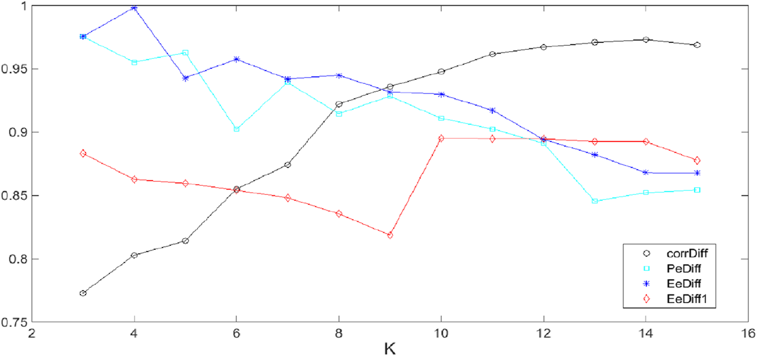$\tau =0.005$ and $\alpha =4000$ fixed).

The 20 illustrations in Figures 6–8 indicate that the component $sc5$ is separated well in almost all instances regardless of the correctness of the decomposition effect. To determine the reason, let us examine the $sc5$ component in all of the illustrations to observe the signal’s characteristics. The component of this signal amplitude is higher than the other components, and the component covers the entire time domain. Furthermore, the separation is significant in the frequency domain of each illustration showing the decomposition effect. The VIMF component corresponding to the component $sc5$ shares the highest correlation with the original signal upon investigation of the correlation coefficients between each VIMF component and the original signal obtained at each time. Therefore, employing the correlation coefficients of this VIMF component-related term as an index is feasible and appropriate in the comparison of the VMD decomposition effect.

For cases involving a combination of different parameters, the envelope entropy of the VIMF component with the strongest correlation with the original signal is recorded as $E{E}_{\max }$ , which is employed as the fitness function for the VMD parameter optimization. The results obtained by the optimization method are listed in Table 1. The $E{E}_{\max }$ obtained via the VMD processing under different parameter combinations is recorded as $E\mathrm{e}Dif{f}_1$ , and the results of similar calculations are also plotted in Figures 12–14.

Figure 13.

VMD decomposition effect evaluation indexes vary with different parameter $\alpha$ values (with $\tau =0.005$ and $K=8$ fixed).

Figure 14.

VMD decomposition effect evaluation indexes vary with different parameter $\tau$ values (with $\alpha =4000$ and $K=8$ fixed).

The three figures indicate that the effect evaluation indexes of the VMD method for signal $S_7$ vary with the change of each single parameter value from the different sides, but the actual situation is much more complicated. First, the correlation coefficient between $u_{sum}$ and the original signal, $corrDiff$ , is investigated. The index $corrDiff$ obtained by the VMD method shows an increasing trend when the parameter K increases gradually and the other two parameters are fixed. Furthermore, $corrDiff$ shows a decreasing trend when the parameter $\alpha$ increases gradually and the other two parameters are fixed, but the correlation coefficient is relatively large in general. Meanwhile, $corrDiff$ shows an essentially indeterminate trend when the parameter $\tau$ increases gradually and the other two parameters are fixed, but the correlation coefficient is relatively small in general. These findings may be attributed to the $\mu =4$ set in Equation (10) that is larger than the two cases of $\mu =1$ and $\mu =2$ . The noise amplitude also increases, which further complicates the signal decomposition.

Second, the permutation entropy of the difference between $u_{sum}$ and the original signal, $P\mathrm{e}Diff$ , is investigated. The index $P\mathrm{e}Diff$ obtained by the VMD method shows an overall decreasing trend when the parameter K increases gradually and the other two parameters are fixed. In some cases, the signal entails an insufficient decomposition. In particular, when the parameter K is less than the proper value of 8, this situation leads to the increase in the correlation coefficient for the difference between $u_{sum}$ and the original signal, which is caused by the modal aliasing of the decomposed signal components. In other cases, the signal entails an excessive decomposition. In particular, when K is greater than the proper value of 9, this situation leads to the increase in reconstruction errors and the decrease in the correlation coefficient of the difference between $u_{sum}$ and the original signal. Furthermore, the $P\mathrm{e}Diff$ obtained by the VMD method shows an overall increasing trend when the parameter $\alpha$ increases gradually and the other two parameters are fixed. This finding may be related to the adjustment effect of the modal frequency bandwidth control parameter $\alpha$ . In particular, the larger the $\alpha$ , the narrower the frequency band of each VIMF component centering on the center frequency. The other frequency bands are likely error frequency band(s). Moreover, the smaller the error, the more accurate the VMD variational modal frequency components can be obtained, and the higher the PE value of the remaining error component $n_r$ . However, the subsequent waveform gradually stabilizes after increasing only to a certain extent and remains constant. Moreover, the $P\mathrm{e}Diff$ obtained by the VMD method shows an overall decreasing trend when the parameter $\tau$ increases gradually and the other two parameters are fixed. However, the subsequent waveform gradually stabilizes and remains constant.

Third, the envelope entropy of ${\mu }_1$ denoted by $E\mathrm{e}Diff$ is investigated. The index $E\mathrm{e}Diff$ obtained by the VMD method shows an overall decreasing trend when the parameter K increases gradually and the other two parameters are fixed. However, this index is neither the smallest parameter K nor the largest one that can contribute to the determination of the best decomposition effect according to the actual situation. Rather, the value of 8 or 9 for the parameter K in the middle position may lead to the best result, suggesting that the method in Ref. ⁵⁵ does not make sense in this case. The $E\mathrm{e}Diff$ obtained by the VMD method shows an overall decreasing trend when the parameter K decreases and increases and the other two parameters are fixed. The situation is similar when the parameter $\alpha$ increases gradually. Therefore, the $E\mathrm{e}Diff$ defined by this method is not suitable as a term of the fitness function.

Finally, the envelope entropy of the VIMF component with the strongest correlation with the original signal, denoted by $E\mathrm{e}Diff1$ , is investigated. The term $E\mathrm{e}Diff1$ obtained by the VMD method shows an increasing followed by a decreasing trend when the parameter K increases gradually and the other two parameters are fixed. Here, the term reaches a minimum near the parameter K = 9, which seems consistent with the practical situation to a certain extent, i.e., the value 8 or 9 of the parameter K in the middle position may lead to the best decomposition result. Similar increasing and decreasing trends are observed when the parameter $\alpha$ or $\tau$ increases. Therefore, the $E\mathrm{e}Diff1$ defined in the method is suitable as a term of the fitness function.

The comparative observation has ignored two or more interactions that can affect the parameters, and this aspect may be only the result of the local relative optimal results but not the global best results.

In summary, the influence of the three parameters (number of modal layers K, modal frequency bandwidth control parameter (or quadratic penalty term) $\alpha$ , and noise tolerance $\tau$ ) on the decomposition effect evaluation indexes of $corr$ , $P{E}_n$ , $E{E}_{u1}$ and $E{E}_{\max }$ are extremely complicated. Optimizing the problem by simply using an evaluation index is inadequate. To a certain extent, the larger the correlation ( $corr$ ) between $u_{sum}$ and the original signal, the higher the assurance that the decomposed signal “is loyal to” the original signal, and a relationship that is too far from the original signal can be avoided. However, this term is not entirely the case of “the larger, the better.” For the signal containing a high volume of noise, the denoising function of VMD may lead to “more similar in shape” between the decomposed signal and the pure signal of the original signal but “not so similar” between the decomposed signal and the specific noise detail. To a certain extent, the larger the permutation entropy ( $P{E}_n$ ) of the difference between $u_{sum}$ and the original signal, the better the denoising effect. This condition renders the pure signal in the noised signal to be separated perfectly, and the residual is mainly a noise component at the last item. Similarly, the term is not entirely the case of “the larger, the better.” In some cases, the noise is separated from the original signal, but different modal frequency components are mixed. Moreover, the smaller the envelope entropy ( $E{E}_{\max }$ ) of the VIMF component, the stronger the correlation with the original signal. However, this term is not entirely the case of “the smaller, the better.” In other cases, the small $E{E}_{\max }$ corresponds to the signal denoising separation effect, but the number of modal layers K is inappropriate, which may lead to the phenomenon of insufficient or excessive decomposition. Thus, a comprehensive consideration approach should be developed to overcome the above deficiencies.

4. Improved parameter-optimized VMD method

For nonlinear and nonstationary signals without prior modal information, in view of the aforementioned single-objective optimization method’s failure to obtain a robust VMD parameter of the number of modal layers K, the modal frequency bandwidth control parameter (or quadratic penalty term) $\alpha$ and the noise tolerance $\tau$ can be utilized.

Multi-objective functions should be employed to restrict each of the objective functions and optimize the VMD parameters. As discussed in Section 3.2, it is time-consuming to determine the optimal VMD parameters by using different parameter combinations and performing VMD processing to obtain different decomposition effect measurement indicators. Subsequently, comparing and weighing comprehensively the functions is not entirely objective. Consider each experiment in which K, $\alpha$ , and $\tau$ serve as different parameters for combination. A VMD processing is conducted, and different decomposition effect evaluation indexes are calculated and compared. Taking the calculation investigation of a signal with 1000 sampling points as an example, 4 s is needed for each VMD processing to be performed. Moreover, 0.5 s is required to calculate each of the signal PE values. For the time being, by ignoring the time-consuming characteristics of the other calculations, the value of the parameter K in the external iterative loop varies from 2 to 15 (step length is 1) at 14 times in total, and the value of the parameter $\alpha$ in the middle iterative loop varies from 20 to 10000 (step length is 20) at 500 times in total, and the value of the parameter $\tau$ in the internal iterative loop varies from 0 to 0.005 (step length is 0.0001) at 51 times in total. Thus, (4+0.5) × 14 × 500 × 51 = 1606500 s is needed to calculate each of the terms of the fitness function value. That is, the calculations of the three terms of fitness function value discussed here take approximately 1338.75 hours, less the comparison to find the extrema. Obviously, this method of conventional comparative observation not only fails to find the optimal result but may be inefficient.

The MOPSO algorithm is a multi-iteration optimization algorithm based on population inspiration, and it has strong local and global optimization capabilities, ⁶¹ which is suitable in determining the optimal VMD parameters. Therefore, on the basis of the introduction of the MOPSO algorithm, an adaptive VMD parameter-optimized method based on the multi-objective particle swarm algorithm is proposed in this section to adaptively determine the proper selection of VMD parameters in the process of identifying the characteristics of nonlinear and nonstationary signals.

4.1. Multi-objective particle swarm optimization algorithm

Optimization problems in the real world are often multi-attribute in nature, and two or more goals are generally optimized at the same time. The most excellent development of a country involves many aspects, such as rapid economic growth, stability of social order, and environmental protection and improvement. ⁶² The two optimization goals of rapid economic growth and social order stability here are complementary and mutually reinforcing—a virtuous circle—and are usually consistent.

In many cases, two or more goals optimized at the same time are not only complementary but also interactive yet conflicting. For example, in the production activities of a company, the quality of the product conflicts with its production cost. ⁶² The corporate leadership usually comprehensively considers the conflicting subgoals to achieve the optimization of the overall goal. That is, each subgoal is considered to be compromised to the plan and the production management. ⁶² Such a problem of comprehensive and compromised consideration of multiple sub-objectives is often called a multi-objective optimization problem.

For a single-objective optimization problem, only a single optimal solution exists, and it can be obtained using relatively simple and commonly used mathematical methods. However, for a multi-objective optimization problem, each objective restricts the other objectives, and the performance of a single objective is often improved at the cost of losing the performance of the other objectives. Determining a solution to optimize the performance of all objectives is impossible. ⁶² One of the considered principles is the Pareto efficiency principle, referring to an ideal state of resource allocation. That is, for an inherent group of people and resources assumed for allocation, when the allocation state changes from one to another, one person at least becomes better with the assurance of the situation that no other person becomes worse. The multi-objective evolutionary algorithm (MOEA) can optimize the multi-objective problem (MOP) according to the Pareto principle and other strategies. As one of the MOEAs, MOPSO is featured with the advantages of fewer parametric settings, good convergence at high speed, and simple calculation. As such, MOPSO is widely used to solve multi-objective optimization problems, such as color image fusion, ⁶³ location identification of automatic voltage regulators in distribution networks, ⁶⁴ network security optimization, ⁶⁵ multi-objective calibration of reservoir water quality modeling, ⁶⁶ hybrid renewable energy system design, ⁶⁷ structured optimization of airborne radar radome, ⁶⁸ satellite image pixel classification, ⁶⁹ earthquake emergency response strategy optimization, ⁷⁰ and multi-feature selection and classification of image or text. ⁷¹ For the convenience of problem description, this section introduces some basic concepts of multi-objective optimization problems, the framework, and the steps of the MOPSO algorithm.

4.1.1. Basic concepts of multi-objective optimization problems

4.1.1.1. Global optimum (minimum)

Suppose a single-objective function f, $\mathrm{\Omega }\subseteq R^D\to R$ , $\mathrm{\Omega }\ne \varnothing$ , if and only if it satisfies the condition

$\forall {\overrightarrow{x}}^{*}\in \mathrm{\Omega },f\left({\overrightarrow{x}}^{*}\right)\le f\left(\overrightarrow{x}\right)$

(24)

Then, the specific function value of f, $f^{*}\triangleq f\left({\overrightarrow{x}}^{*}\right)>-\infty$ , is called the global optimal (or minmum). Here, ${\overrightarrow{x}}^{*}$ is the global optimum (minimum) solution, and the set $\mathrm{\Omega }$ is the feasible solution space $\mathrm{\Omega }\in S$ , where $S$ is the entire feasible solution space. ⁷² As the optimization problem of the global maximum can be converted into an optimization problem of the minimum by adding a minus sign or the conversion of other decreasing functions, the succeeding discussions shall only call the global minimum problem a global optimal problem. As the optimization problem of the global maximum can be converted into a minimum optimization problem by adding a minus sign or the conversion of other decreasing functions, all of the global optimal problems can be regarded as global mini-mum problems in the succeeding discussions. ⁷²

4.1.1.2. Multi-objective optimization problem

As aforementioned, the multi-objective optimization problem in specific engineering applications involves reasonable compromise considerations of multiple objectives with various competitive relationships and mutual inhibitions. Without loss of generality, an optimization problem with a real D-dimensional decision space is investigated. A parameter set P must satisfy the following relationship:

$\begin{array}{l}\underset{P\in X}{\mathit{Min}}F\left(X\right)={\left[f_1\left(X\right),f_2\left(X\right),\cdots ,f_n\left(X\right)\right]}^T\\ \begin{array}{ll}s.t.& g_i\left(X\right)\ge 0,i=1,2,\cdots ,p\\ & h_j\left(X\right)\ge 0,j=1,2,\cdots ,q\end{array}\end{array}$

(25)

where $F={\left\{f_1,f_2,\cdots ,f_M\right\}}^T$ is a function vector with M optimization objectives and called objective function or fitness function, $g_i\left(X\right)$ and $h_j\left(X\right)$ are constraint functions, $X={\left\{x_1,x_2,\cdots ,x_D\right\}}^T$ is a vector with D decision variables, and $\overrightarrow{x}=\{x|x\in R^n,$ $g_i\left(x\right)\ge 0,$ $h_j\left(x\right)=0,i=1,2,\cdots ,p,j=1,2,\cdots ,q\}$ is a feasible solution space of Equation (25). ⁷³

The decision vector x corresponds to a point in the D-dimensional decision variable space $R^D$ , and the fitness function $F\left(x\right)$ corresponds to a point in the M-dimensional optimization objective function space $R^M$ ; i.e., the fitness function $F\left(x\right)$ corresponds to a mapping from the D-dimensional decision variable space to M-dimensional optimization objective function, $f:R^D\to R^M$ ⁶² . In the actual optimization problem $X=\left\{x_1,x_2,\cdots ,x_D\right\}$ , a set of vectors designated by the designer (decision maker) based on actual cases is called a solution of the optimization problem. Moreover, a set of decision variables that satisfy all constraints can be called a feasible solution. ⁶² The feasible solutions to an optimization problem is infinite, and the methods to obtain the optimal (minimum) conditions for the multiple objectives include the multi-objective weighting method that assigns different weights to these objectives, the Pareto optimal solution method, and so on.^62,72,73

4.1.1.3. Pareto optimal

The MOP-optimized solution exists in the form of compromise substitution, which is called the Pareto optimal set. Each objective component of any non-dominated solution in the Pareto optimal set can only be improved by deteriorating at least one of the other objective components. ⁶²

For any $\overrightarrow{x}\in \mathrm{\Omega }$ , $I=\left\{1,2,\cdots ,D\right\}$ , if a special solution ${\overrightarrow{x}}^{*}$ satisfies the conditions of

${\forall }_{i\in I}\left[f_i\left(\overrightarrow{x}\right)=f_i\left({\overrightarrow{x}}^{*}\right)\right]$

(26)

or at least one $i\in I$ exists such that

$f_i\left(\overrightarrow{x}\right)>f_i\left({\overrightarrow{x}}^{*}\right)$

(27)

then the special solution ${\overrightarrow{x}}^{*}$ in $\mathrm{\Omega }$ is called the Pareto optimal. ⁶² In other words, if a certain feasible solution space ${\overrightarrow{x}}^{*}$ improves at least one optimization objective without deteriorating any other optimization objective, then ${\overrightarrow{x}}^{*}$ can be regarded as the Pareto optimal. ⁶²

4.1.1.4. Pareto dominating

If $\overrightarrow{u}=\left[u_1,u_2,\cdots ,u_D\right]$ and $\overrightarrow{v}=[v_1,v_2,\cdots$ $,v_D]$ are two feasible solutions to a problem with only two optimization objectives $f_1$ and $f_2$ , respectively, if and only if the two conditions, namely,

① all of the objectives function of the feasible solution $\overrightarrow{u}$ are not worse than that of $\overrightarrow{v}$ , that is, $f_1\left(\overrightarrow{u}\right)\le f_1\left(\overrightarrow{v}\right)$ and $f_2\left(\overrightarrow{u}\right)\le f_2\left(\overrightarrow{v}\right)$ , and

② at least one objective function of the feasible solution is superior to that of, that is, $f_1\left(\overrightarrow{u}\right)<f_1\left(\overrightarrow{v}\right)$ or $f_2\left(\overrightarrow{u}\right)<f_2\left(\overrightarrow{v}\right)$ are all met, then $\overrightarrow{u}$ is Pareto-superior to $\overrightarrow{v}$ , or $\overrightarrow{u}$ is Pareto-dominating of $\overrightarrow{v}$ , and it is denoted as $\overrightarrow{u}\prec \overrightarrow{v}$ .

4.1.1.5. Pareto optimal set (non-inferior optimal solution)

For a given multi-objective optimization problem $\overrightarrow{F}\left(x\right)$ , its non-inferior solution set $P^{*}$ is defined as follows ⁴⁶ :

$P^{*}=\left\{x\in \mathrm{\Omega }|\neg \exists x^{\prime }\in \mathrm{\Omega },\overrightarrow{f}\left(x^{\prime }\right)\underset{\_}{\prec }\overrightarrow{f}\left(x\right)\right\}$

(28)

4.1.1.6. Pareto front

For a given multi-objective optimization problem $\overrightarrow{F}\left(x\right)$ and its non-inferior solution set $P^{*}$ , the Pareto front is defined as

$P{F}^{*}=\left\{\overrightarrow{u}=\overrightarrow{f}=\left[f_1\left(\overrightarrow{x}\right),f_1\left(\overrightarrow{x}\right),\cdots ,f_M\left(\overrightarrow{x}\right)\right]|x\in P^{*}\right\}$

(29)

That is, a special solution in the Pareto front always dominates any feasible solution in the feasible solution space.^72,73

In general, finding the analytical expressions containing the frontier (line or surface) of these Pareto optimal solution set is impossible. Only through constant calculation and a search of feasible solutions $\mathrm{\Omega }$ and corresponding optimization objectives $f\left(\mathrm{\Omega }\right)$ until their numbers are sufficiently large can the Pareto front be further generated.^72,73

The abovementioned analysis only explains the related concepts of the optimization problem with two objectives. Furthermore, the term of two objectives can be extended to that of multi-objectives according to the need of a specific problem, which is not repeated in this section due to the paper’s space constraints.

The Pareto dominance-related problems of the optimization problem with two objectives are plotted in Figure 15 to be able to explain in detail the Pareto optimal front and the Pareto dominance problem. With the optimization objectives $f_1$ and $f_2$ serving as the horizontal and vertical axes of the coordinates, some feasible solutions A, B, C, D, E, and F are obtained according to the relevant algorithm and plotted in the figure according to the fitness function value. ⁶¹ These elements constitute a feasible solution set.

Figure 15

Pareto dominance and Pareto optimal front Ref. ⁷²

From the perspective of the objective space, the hollow circle F is dominated by the hollow circles D and E and the filled circles A, B, and C. The hollow circles D and E are dominated by A, B, and C. That is, F is dominated by all other feasible solutions, and solutions D, E, F are not Pareto optimal solutions. The filled circles A, B, and C are not dominated by each other, and they are not dominated by other feasible solutions. The search process is continued until no feasible solution can dominate A, B, and C. Then, the connection of A, B, and C constitutes a Pareto front.

4.1.2. Framework and steps of the MOPSO algorithm

Coello ⁷⁴ compared PSO with other evolutionary algorithms and proposed that the PSO with the Pareto sorting scheme may be a direct and effective method to expand the processing of multi-objective optimization problems.

The historical record of the best solution found by the particles (i.e., individuals) can be used to store the non-dominated solutions generated in the past history, which is similar to the elitism concept used in other evolutionary computing methods. ⁷⁴ Moreover, the combination of the global search mechanism and the external archiving of the non-dominated vectors discovered in history can encourage the iterative process to converge into a more optimal dominated solution and into non-dominated solutions. ⁷⁴ The external file can also be used to store the local and global optimal solutions generated in the iterative process. The external file contains individuals that are not dominated by any other particles and individuals that dominate some feasible solutions in the external set.

The flowchart of the MOPSO algorithm is shown in Figure 16. The specific steps are as follows ⁷⁴ :

(1) Particle population initialization: Randomly specify the initial position and velocity of the particle according to the value range.

(2) Preliminary calculation: Calculate each fitness function value according to the regulations and the initial position of the particles. Calculate the non-dominated solution and store it in the Rep as the current external file.

(3) Local optimization: Define each particle coordinate according to its fitness function value. Then, the position in the objective function is formed into a hypercube, and the initial individual optimal position Pbest and the global optimal position Gbest of the particle are determined.

(4) Update particle position and velocity and update Pbest : Continuously compare and search for Pbest in a supposed value range following the constraints. Iteratively calculate the position and velocity of each particle according to the formula (the same as the PSO algorithm). Update the individual’s historical optimal value and historical maximum Pbest after comparison.

(5) Maintenance of external file Rep, and comparison and selection of Gbest : Comprehensively compare the objective function values of all particles, add the non-dominated solution generated in this iteration to the external file Rep , and update the overall optimal value and the overall optimal position Gbest.

(6) Judge whether the iteration can be stopped: When the number of iterations has not reached MaxIter and the Pareto optimal value has not been found, repeat step (3), and the iteration continues until the number of iterations reaches MaxIter or the Pareto optimal value is found. Then, the iteration stops, and the obtained external file set Rep is the Pareto optimal solution set via the algorithm.

Figure 16.

Flowchart of the MOPSO algorithm Ref. ⁷²

In the entire iterative process of the optimization algorithm, either the global optimal solution or the selection of the particle’s historical optimal solution is expected to greatly impact the optimization result. In each iteration, a new global optimal solution is generated, and other particles are guided to move (or fly) in space or constrained space based on the position of the global optimal solution.^74–76 In the optimization process of MOPs, a set of global optimal solutions is generated in each iteration, and only the optimal solution selected among them may guide the next particle flight to the convergence direction. Lalwani ⁷⁵ greatly contributed to the selection of external files, mutation strategies, and constraint control to improve the effectiveness of MOPSO, established a set of optimization problem test functions, and formulated evaluation indicators regarding the advantages and disadvantages of the algorithm, such as iteration distance, error rate, and spatial distribution. Although the indicators are convenient and effective and eventually applied in this study, they are not detailed here given the paper’s space limitations.

4.2. Proposed VMD parameter optimized method

As mentioned in Section 3.2, $corr$ , $P{E}_n$ , $E{E}_{u1}$ and $E{E}_{\max }$ , etc., are among several decomposition effect evaluation indicators that can be used to search for the best fitness function value, each of which serving as the optimization objective to search for the best decomposition effect. However, these indicators are all biased because of the mutual restriction relationship among them. An adaptive VMD parameter optimization method that takes into account the mutual constraints of decomposition effect evaluation indicators should be urgently developed to identify the numerous nonlinear and nonstationary signals in nature (especially bridge GNSS dynamic monitoring data) via VMD. In general, the strategy of the adaptive method is to use several search rules to explore and find the optimal parameters, including the construction of evaluation indicators and the selection of search methods. The MOPSO algorithm introduced in Section 4.1 is an ideal searching and optimization method. Hence, an adaptive VMD parameters optimization method based on MOPSO is proposed in this study.

The proposed method employs $corr$ , $P{E}_n$ and $E{E}_{\max }$ as the multi-objective fitness functions and conducts an adaptive optimization of the three VMD parameters of K, $\alpha$ , and $\tau$ via the MOPSO algorithm. This approach is called adaptive variational modal decomposition parameter optimization method based on the MOPSO algorithm, abbreviated as AVMDbMOPSO, which is mathematically expressed as

$\{\begin{array}{l}fitness=\min \left\{corr;P{E}_n;E{E}_{\max }\right\}\\ \begin{array}{ll}s.t.& K=2,3,\cdots ,15\\ & \alpha \in \left[500,10000\right]\\ & \tau \in \left[0,0.05\right]\end{array}\end{array}$

(30)

where $fitness$ represents the aforementioned objective function. Three objective functions are considered, and the result of the MOP solving process corresponds to the three objectives to be checked and balanced with respect to each other, thus achieving a compromise. The three decision variables after $s.t.$ are the value ranges of K, $\alpha$ , and $\tau$ , which can also be regarded as constraint functions. The implementation steps of the AVMDbMOPSO are as follows:

• (1) Input the nonlinear and nonstationary signal $x\left(t\right)$ , assign the value range of the VMD parameters, and assign the values of the MOPSO parameters, such as the times of iterations MaxIter and the number of particle populations nPop.

• (2) Initialize the position and velocity of the MOPSO algorithm according to the value ranges of the VMD parameters, and calculate a set of initial particle values.

• (3) Perform VMD decomposition on the signal by using the assigned parameter values. Then, calculate the fitness function of each particle position corresponding to the state, compare and obtain the fitness value, and update the external file with the non-inferior dominance solution that meets the requirements.

• (4) Update the particle position and velocity, and adjust the optimal fitness function value and optimal parameter value.

• (5) Judge whether the iteration stop condition is reached, that is, whether the number of iterations iter reaches MaxIter or whether the Pareto optimal value is found. If the condition is not reached, then set iter = iter +1, loop to step (3), and continue the iteration. Otherwise, stop the iteration and obtain the external file set.

• (6) Perform VMD decomposition on the signal by using the obtained VMD parameters in the external archives to obtain the correct and effective frequencies and other characteristic parameters.

The external file set here has multiple combinations of optimal values, and the parameters also have multiple optimal values.

4.3. Simulation experiment and verification

The experimental analysis on the multi-component frequency modulation signal with $\mu$ = 2 in Equation (10) is performed, and the VMD parameter optimization is conducted using the new proposed method in Section 4.2. The relevant parametric settings are as follows: the value range of the VMD parameter here is taken according to Equation (3–29), the MOPSO parameter MaxIter is set to 50, the nPop is set to 50, and the number of external file sets nPS is set to 10. Figure 17(a) shows the multi-objective value of the obtained multi-objective optimized external file set. The values of $corr$ and $P{E}_n$ in the obtained result represent the objective values transformed according to Equation (23). These variables should be converted into normal ones. The back-converted results are shown in Figure 17(b). As shown in the illustration, the mutual restriction of the three objectives can reach a good compromise.

Figure 17.

The three-objective optimization result graph via AVMDbMOPSO processing.

The optimized VMD parameter sets are listed in Table 2. The figure and table both show that the evaluation indicators of the decomposition results of VMD tend to be close after multi-objective optimization, but they are different. In the optimized VMD parameters, the parameter K value is all 9, the parameter value $\alpha$ ranges from 2000 to 4000, and the $\tau$ value is always 0. These results indicate that although the selected VMD decomposition evaluation indicators are mutually restricted and exclusive, the multi-objective equilibrium optimization of MOPSO can contribute to the achievement of a compromise. The result of the compromise is that, although the values of the parameters are different, the values of K in the external file set are all 9, which is highly gratifying.

Table 2.

The optimal VMD parameters list of the signal $S_7$ processed by AVMDbMOPSO.

Experiment	The No. of the external file set	K	$\alpha$	$\tau$	The No. of the external file set	K	$\alpha$	$\tau$
A	1	9	2048.6	0	6	9	2164.3	0
	2	9	3120.7	0	7	9	2327.3	0
	3	9	2134.1	0	8	9	1772.8	0
	4	9	1573.4	0	9	9	2102.5	0
	5	9	1892.8	0	10	9	1968.0	0
B	1	9	3344.6	0	6	9	3487.9	0
	2	9	5385.4	0	7	9	1612.9	0
	3	9	3554.7	0	8	9	4057.6	0
	4	9	3332.6	0	9	9	3898.5	0
	5	9	4955.4	0	10	9	5209.1	0

The ten sets of parameter combinations are subjected to VMD decomposition. Each set can gain a good VMD decomposition effect, one of which is drawn in Figure 18. The VMD decomposition effect is clearly good, and the five frequency components and noise items of the original signal are well identified. In the VMD algorithm analyzed above, the proper selection of the K is proven to be the most important parameter, followed by $\alpha$ , and finally by $\tau$ . Moreover, when the K value is properly determined and the $\alpha$ value varies within a certain range, a good VMD decomposition effect can be obtained, which is consistent with the previous analysis.

Figure 18.

Time-frequency diagram obtained by VMD with optimized parameter combination.

As for the parameter $\tau$ , the optimization results obtained by the AVMDbMOPSO method are all 0, which verifies the correctness of the aforementioned assumptions. That is, for a nonlinear and nonstationary signal with a large amplitude noise, the appropriate setting of the parameters plays the role of noise adjustment and suppression. When the noise amplitude is not sufficiently large, the default configuration of 0 or a small value is appropriate, which is consistent with the analysis in Section 3.1.

The same experimental analysis on the multi-component frequency modulation signal $S_7$ is performed, and the VMD parameter optimization is also conducted with the same method. Optimization results similar to those shown in Figures 15 and 16 are also obtained. However, due to the space limitations of this paper, the details are not discussed in this section. Only the optimized VMD parameter sets are listed in Table 2 (lower half of the tabulation). A relatively consistent parameter modal number K occurs in the optimization result of Experiment B, each of which is 9. The value of $\alpha$ varies from 1500 to 5500; although the details are different from those in Experiment A, the conclusion is the same. Furthermore, a good decomposition effect can be obtained with the optimized parameter combination obtained in Experiment B for the VMD processing on the signal $S_7$ , which is consistent with the conclusion of Experiment A. This result indicates that the proposed method is repeatable, and the effect is good.

In summary, the AVMDbMOPSO method can effectively and reliably perform a time–frequency analysis on nonlinear and nonstationary signals, and it may help to gain a more perfect decomposition effect, suggesting its superiority to the existing VMD parameter optimization methods. The AVMDbMOPSO method is expected to guarantee effective feature identification and analysis of actual bridge GNSS monitoring data.

5. Application in dynamic characteristic identification of bridge GNSS monitoring data

To assess the effectiveness and advantages of the proposed VMD parameter optimization strategy, this study utilizes the same GNSS monitoring data from the Sutong Yangtze River Highway Bridge as referenced in ¹⁸ . The Sutong Bridge is a double-tower, double-plane steel box girder cable-stayed structure spanning 8146 m in total length, with a main span of 1088 m and a main cable tower reaching 300.4 m in height. It is situated downstream of the Yangtze River, connecting Nantong and Suzhou in eastern Jiangsu Province, and is frequently affected by summer typhoons. Combined with daily and seasonal temperature fluctuations, these environmental factors significantly challenge the precise positioning of the superstructure. To meet the high standards of geometric alignment, elevation control, dynamic response monitoring, and tower deviation assessment during construction, a remote real-time dynamic monitoring system based on GNSS technology was established. This system continuously captures the geometric and structural behavior of both towers and girders in real time. ²⁵ GNSS receivers were installed on the tower tops immediately after the roof sealing. Given that the natural frequency of such large cable-stayed bridges is typically below 5 Hz, a 10 Hz sampling rate was adopted in accordance with the Nyquist theorem, enabling effective acquisition of vibration signals and contributing to the safe construction of the bridge.

The bridge GNSS monitoring data series was transformed into the bridge axis coordinate system, and then averaged. Then the x, y, and z coordinate sequences are all actually parallel or perpendicular to the bridge axis, which will lead to the analysis results more consistent with the actual situation of bridge vibration. The data were collected from the GNSS monitoring point in the bridge axis coordinate system on the north bridge tower. A section of x-direction monitoring time series data starting at 20:32 on December 26, 2006, with a duration of 500 s was analyzed. Then this x sequence was decomposed by AVMDbMOPSO method. The setting of the proposed parameters here is the same as that in Section 4.3. The obtained multi-objective value of the external file set of the multi-objective optimization (an inverse function transformation is conducted) is shown in Figure 19. The mutual restriction of the three objectives is also well compromised. The optimized VMD parameter sets are listed in Table 3. The figure and table both show that the evaluation indexes of the decomposition effect of the VMD decomposition on the bridge monitoring data tend to be close after multi-objective optimization, but they are different. In the optimized VMD parameters, the value of K is always 10, the value of $\alpha$ ranges from 1200 to 5800, and the value of $\tau$ ranges from 0.0003 to 0.0010.

Figure 19.

Three-objective optimization result via AVMDbMOPSO processing on the bridge GNSS monitoring data.

Table 3.

The optimal VMD parameters list of the signal 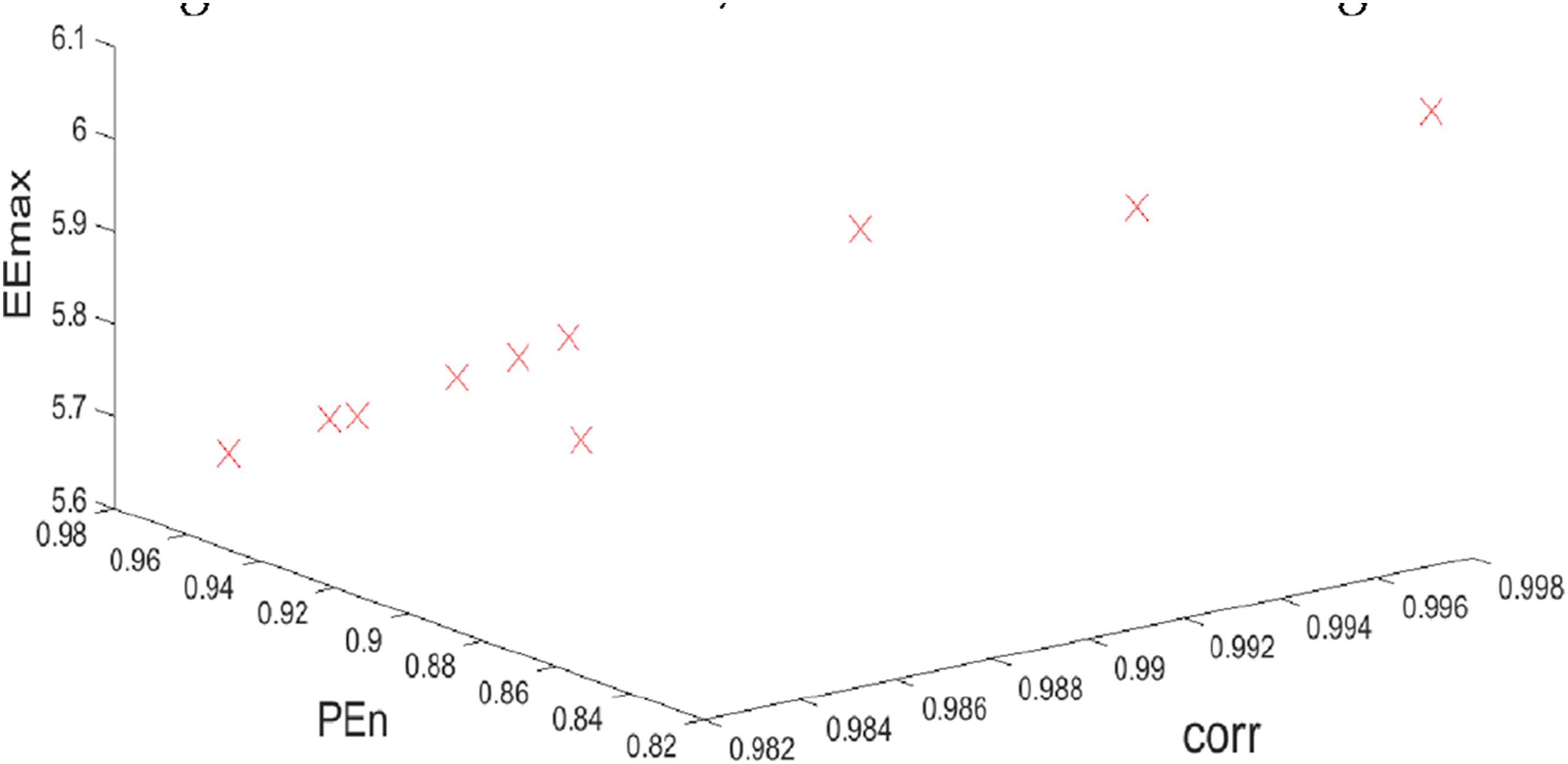$S_7$ processed by AVMDbMOPSO.

The No. of the external file set	K	$\alpha$	$\tau$	The No. of the external file set	K	$\alpha$	$\tau$
1	10	5024.1	0.0007	6	10	3642.4	0.0003
2	10	3350.8	0.0005	7	10	2327.3	0.0008
3	10	5749.4	0.0007	8	10	3280.6	0.0004
4	10	4826.9	0.0006	9	10	2238.3	0.0010
5	10	4081.0	0.0007	10	10	1233.7	0.0007

These results indicate that although the selected VMD decomposition evaluation indicators are mutually restricted and exclusive, the multi-objective equilibrium optimization of MOPSO can contribute to the achievement of a compromise. The result of K value (always 10) verifies that the AVMDbMOPSO method is robust to any signal analysis unlike the unstable K value optimization results of some existing methods.

The ten sets of parameter combinations are subjected to VMD decomposition. Each set of data can gain a good VMD decomposition effect, one of which is drawn in Figure 20. For the bridge GNSS monitoring data with unknown prior frequency information, especially the number of modal layers K, the VMD parameters can be optimized to such a result by adopting the proposed method. In the time–frequency diagram, the VIMF1 component is indeed the irregular fluctuation of the signal as a whole, and the trend is shown in Figure 20. Moreover, the VIMF2 component has an obvious vibration frequency of 0.156 Hz whose amplitude can reach 7.6. The conclusions are the same as the QGA-ASR analysis in Ref. ¹⁸ . Furthermore, low amplitudes at 0.744 and 2.544 Hz can be observed in the subsequent VIMF components. This trend may be a multi-order frequency characteristic of the bridge vibration, which requires further analysis and verification.

Figure 20.

Time–frequency relationship obtained by VMD with optimized parameter combination from VMDbMOPSO.

The proposed method was used to decompose the other parts of the x and y coordinate sequences for the point. AVMDbMOPSO has a similar decomposition performance. In addition, the main natural vibration frequencies in the x- and y-directions in each section is 0.156 Hz. The graphs and results obtained in these cases are omitted to save space. The same frequency of the bridge vibration in the x- and y-directions was obtained in other section from the two monitoring points in a single hour; hence, the bridge was safe at that time.

6. Discussion

Bridge GNSS monitoring data exhibit complex nonlinear and nonstationary characteristics, making frequency extraction challenging with any single method. This study contributes a practical decision framework for method selection and proposes an adaptive VMD parameter optimization approach (AVMDbMOPSO) to address this limitation. The key contribution is the AVMDbMOPSO method, which automatically optimizes VMD decomposition parameters using multi-objective particle swarm optimization. This enables accurate frequency extraction from complex, noise-contaminated signals without manual parameter tuning.

Based on our findings, the following application guidelines are proposed:

(1) Regular excitation: FFT or HHT suffices when the main frequency is prominent.

(2) Noisy environments: EMD-based methods, particularly PSEEMD, ¹⁶ are recommended when spectral features are obscured.

(3) Subtle condition changes: The adaptive stochastic resonance method ¹⁸ effectively detects minor frequency shifts near the natural frequency for early damage warning.

(4) Complex multi-modal signals: Standard VMD can extract dominant frequencies when modal layers are known. For uncertain cases, AVMDbMOPSO provides optimized parameters for more accurate decomposition.

In summary, this study provides both theoretical insights and practical tools for bridge GNSS monitoring, with the proposed AVMDbMOPSO method advancing adaptive, high-precision structural health assessment.

Recent “wave-shaped” vibrations observed on the Humen Bridge ⁷⁷ highlight the critical importance of detecting subtle frequency changes. Even minor, long-term frequency shifts may indicate accumulating structural damage that could eventually lead to major events like sudden deck vibrations.

The proposed AVMDbMOPSO method addresses this need by enabling precise frequency extraction in complex scenarios. For sudden vibration events, AVMDbMOPSO optimizes VMD parameters to accurately identify the new dominant modal frequency. When investigating specific causes (e.g., plastic enclosure removal), pre-event GNSS data processed by EMD or PSEEMD ¹⁶ establishes baseline frequencies, while post-event data analyzed via adaptive stochastic resonance ¹⁸ detects any shifts, allowing causal verification.

For routine bridge monitoring under both stable and variable conditions, EMD-based methods, particularly PSEEMD, are recommended to obtain reliable baseline frequencies. These serve as reference points for detecting accumulated “small changes” that inform structural health assessments.

Due to current limitations, full validation across complete bridge lifecycles—from construction to potential failure—remains unrealized. Future work aims to obtain such long-term monitoring data to further validate and expand the applicability of these methods.

7. Conclusion

VMD is an effective time-frequency analysis method for nonlinear and nonstationary signals, demonstrating superior performance in decomposing signals with variable frequencies. However, its main limitation lies in the difficulty of predefining optimal decomposition parameters (e.g., mode number and noise level) without prior signal knowledge.

To address this, how each parameter affects decomposition quality is analyzed, and a MOPSO-based multi-objective optimization framework that automatically determines optimal VMD parameters by balancing multiple evaluation indices is proposed. Case studies validate the method’s effectiveness and reliability, while application to real bridge GNSS monitoring data confirms its practical utility for engineering applications. The robustness of the method with respect to different noise levels, sampling rates, and signal characteristics will be studied and discussed, and whether the optimized parameters are case-dependent will be clarified in future work.