Dynamic obstacle avoidance path planning for collaborative robot based on improved APF-Bi-RRT algorithm

Abstract

In order to enable a collaborative robot to perform path planning and operate more smoothly in environments with dynamic obstacles, a dynamic obstacle avoidance algorithm, named improved APF-Bi-RRT, is proposed by combining an improved Artificial Potential Field (APF) and an improved Bidirectional Rapidly-exploring Random Tree (Bi-RRT). First, a cost function is constructed with the goal of minimizing the angle change of each joint of the robot to select path nodes planned by the Bi-RRT algorithm, reducing redundant nodes and improving path quality. Second, considering the influence of dynamic obstacles on the various links of the robot, the gravitational field function of the artificial potential field method is constructed in the joint space, and the repulsive field function is reconstructed. Finally, the two algorithms are combined, and simulations are conducted in environments with static and dynamic obstacles. The results show that the improved APF-Bi-RRT algorithm enables the collaborative robot to achieve dynamic obstacle avoidance with smooth paths and smooth operation of all joints, which verifies the effectiveness of the algorithm.

Keywords

collaborative robot artificial potential field bidirectional rapidly-exploring random tree dynamic obstacle avoidance path planning

Introduction

Collaborative robot is a new type of industrial robot capable of interacting with humans in shared space or working safely near humans, which is one of the current research hotspots in the field of robotics due to its lightweight and safety features.¹ With the increasing complexity of the workplace, the collaborative robotic arm needs to avoid static obstacles in addition to dynamic obstacles such as carts, staff, etc. In this case, the offline demonstration church spends a lot of manpower, which is not conducive to efficient production, and there are safety hazards, so the problem of dynamic obstacle avoidance path planning for the robot has received extensive attention from the industrial community and the academic community.^2–4

At present, the algorithms commonly used for path planning of the robot include artificial potential field (APF),⁵ velocity potential field (VPF),⁶ Rapid-exploring Random Tree (RRT),⁷ etc. The RRT algorithm is a random algorithm. It takes the starting point as the root node to generate a random tree and expand it to most areas of the space to seek the optimal path.⁸ However, the operation efficiency of RRT algorithm is low and the planned path is not smooth.⁹ Wang Y et al.¹⁰ proposed a strategy for random tree connectivity, a multi-information RRT (MI-RRT-) global path planning algorithm for multi-objective point planning, which improves the algorithm’s operational efficiency. Hu R¹¹ proposed a control method for machine tool-assisted robots based on an improved Rapidly-exploring Random Tree algorithm and Proportional-Integral-Derivative control. The proposed method outperforms traditional methods in terms of performance indicators such as path length, search time, trajectory deviation, and success rate. Specifically, the success rate of this method is 99.87%, the search time is only 0.354 seconds, and the absolute value of the trajectory deviation is only 0.020 meters. Compared with other models, the planning success rate has increased by 17.31%. The APF algorithm makes the target point generate gravity and obstacles generate repulsive force, and the robot moves towards the target point by avoiding obstacles under the action of resultant force.¹² However, the APF algorithm has problems of failing to reach the target and local optimization.¹³ Chen Y et al.¹⁴ added virtual obstacles to make the robotic arm escape from the local minimum state. Xi W et al.¹⁵ proposed an innovative path planning algorithm that uses the path nodes of an improved PRM as virtual target points for the APF algorithm and effectively addresses the inherent flaws of the APF algorithm by piecewise processing of the attractive function and introducing a relative distance factor into the repulsive function. Mi J et al.¹⁶ proposed the MP-RRT algorithm for dynamic obstacles in human-machine collaborative environments. The algorithm significantly reduces conflicts with pedestrians through dynamic risk assessment and sampling strategies, but there is still room for improvement in the smoothness and real-time performance of paths in complex dynamic environments. Yang J et al.¹⁷ effectively improved the speed and quality of path planning by fusing APF with bidirectional RRT (Bi-RRT) algorithm and introducing adaptive step sizes, but the stability and computational efficiency of the algorithm may be challenged in high-dimensional or extremely complex environments.

The Bi-RRT algorithm is an evolution of the RRT algorithm, because of the use of bidirectional search from the starting point and the end point, so the algorithm’s computational efficiency will be greatly improved, but the planned path is still not smooth.¹⁸ Liwei Y¹⁹ proposed an AtBi-RRT algorithm that introduces the concept of target gravity into Bi-RRT and guides the search tree to grow towards the target, thereby reducing the time for path planning. Liu W et al.²⁰ proposed an IDAPF-QRRT* algorithm aimed at achieving efficiency and safety in path planning for mobile robots. The DPF-QRRT* algorithm can quickly generate initial paths, overcome the limitations of traditional algorithms in convergence speed and node redundancy, and introduce an improved APF method to adjust key discrete path points. Enhanced path safety. Wang G²¹ utilized Dijkstra’s algorithm to select key nodes for the path planned by Bi-RRT algorithm, which increased the path smoothness, in addition to utilizing the dynamic window method to achieve dynamic obstacle avoidance for mobile robots. Xiong Z²² et al. proposed Classified RRT* (C-RRT*), an enhanced variant of RRT*. By classifying nodes based on their connection characteristics, customized processes can be executed to enhance the overall architecture and performance. To further optimize the random tree scaling process, a single backtracking selection parent program and sequential reconnection programs are proposed. In addition, a random offset sampling method was introduced to improve the sampling distribution around the obstacles. The proposed algorithm reduced the initial solution calculation time by 53.15% and 63.08% respectively in large obstacles and chaotic experimental environments. The results demonstrated the effectiveness and advantages of the proposed algorithm in improving solution performance and convergence rate. Although Wang G²¹ and Zhang X²² improved the Bi-RRT algorithm to realize dynamic obstacle avoidance, it is only applicable to 2D planar path planning.、

The rest of the paper is organized as follows. Section 2 is the kinematic modeling of UR10 robot. Section 3 uses the bounding ball method to detect the collision between the robot and the obstacle. Section 4 is to improve the Bi-RRT algorithm and APF algorithm, and combine the two algorithms to propose an improved APF-BI-RRT algorithm. Section 5 is to verify the effectiveness of the algorithm through simulation experiments. Section 6 is the conclusion of this paper.

Kinematic modeling of the UR10 robot

This paper takes the UR10 collaborative robotic arm as the research object, as shown in Figure 1. The UR10 robot is a tandem-type robotic with six rotary joints, and each joint can realize ±360° rotation. The structural sketch of the UR10 robot and the D-H coordinate system are constructed, as shown in Figure 2. According to the external dimensions of the UR10 robot and the D-H parameter coordinate system, the D-H parameter table can be listed, as shown in Table 1.

Figure 1.

UR10 robot.

Figure 2.

The D-H coordinate system.

Table 1.

D-H parameter list.

i	Connecting rod turning angle α_i/°	Pole length a_i/m	Connecting rod deflection d_i/m	Joint angle of rotation θ_i/°
1	90	0	0.128	θ₁ (±360°)
2	0	0.6127	0	θ₂ (±360°)
3	0	0.5716	0	θ₃ (±360°)
4	90	0	0.1639	θ₄ (±360°)
5	-90	0	0.1157	θ₅ (±360°)
6	0	0	0.092	θ₆ (±360°)

The transformation from the coordinate system {Oi-1} to {Oi} can be achieved through a homogeneous transformation matrix of four transformations:

T_{i} = R o t (z, θ_{i}) T r a n s (0, 0, d_{i}) T r a n s (a_{i}, 0, 0) R o t (x, α_{i}) = [\begin{array}{c} \begin{array}{c} c θ_{i} \\ s θ_{i} \\ \begin{array}{c} 0 \\ 0 \end{array} \end{array} & \begin{array}{l} - s θ_{i} c α_{i} \\ c θ_{i} c α_{i} \\ \begin{array}{c} s α_{i} \\ 0 \end{array} \end{array} & \begin{array}{c} \begin{array}{c} s θ_{i} s α_{i} \\ - c θ_{i} s α_{i} \\ \begin{array}{c} c α_{i} \\ 0 \end{array} \end{array} & \begin{array}{c} a_{i} c θ_{i} \\ a_{i} s θ_{i} \\ \begin{array}{c} d_{i} \\ 1 \end{array} \end{array} \end{array} \end{array}]

(1)

In equation (1): $c θ_{i} = \cos θ_{i}, s θ_{i} = \sin θ_{i}, c α_{i} = \cos α_{i}, s α_{i} = \sin α_{i}$

From this, the positive kinematic equations of the UR10 robot can be obtained:

{}_{6}^{0}T = {}_{1}^{0}T {}_{2}^{1}T {}_{3}^{2}T {}_{4}^{3}T {}_{5}^{4}T {}_{6}^{5}T = [\begin{array}{l} \begin{array}{l} n_{x} \\ n_{y} \\ \begin{array}{l} n_{z} \\ 0 \end{array} \end{array} & \begin{array}{l} o_{x} \\ o_{y} \\ \begin{array}{l} o_{z} \\ 0 \end{array} \end{array} & \begin{array}{l} \begin{array}{l} a_{x} \\ a_{y} \\ \begin{array}{l} a_{z} \\ 0 \end{array} \end{array} & \begin{array}{l} p_{x} \\ p_{y} \\ \begin{array}{l} p_{z} \\ 1 \end{array} \end{array} \end{array} \end{array}]

(2)

The inverse kinematics of the UR10 robot was solved using the analytical method,²³ where the matrix equations in Eq. (2) were left-multiplied by the inverse matrix, and the expression for the angle of each joint of the robot could be obtained according to the corresponding equivalence of the left and right elements of the matrix.

Collision detection

Except for objects with obvious constraints on their appearance such as spheres and cubes, the vast majority of obstacles are irregular and their appearance contours contain a large amount of information, so it is not desirable in terms of time cost to perform obstacle avoidance planning after their complete identification, for this reason, the obstacle model needs to be simplified. In this paper, the bounding sphere is used to simplify the obstacles, and the robotic arm can be abstracted as a cylindrical modelliterature²⁴, as shown in Figure 3. The radius of the enclosing sphere is R1 and the radius of the cylindrical model is R2.

Figure 3.

Collision detection between robot and obstacle.

Assuming that the coordinates of the center points of the two ends of the connecting rod are A (x_A, y_A, z_A), B (x_B, y_B, z_B), the coordinates of the center of the sphere O (x_O, y_O, z_O), and the projection point of the center of the sphere O on the straight line AB is O′ (x_O’, y_O’, z_O’), the equations for the distance of the center of the sphere to the straight line AB as well as the distances to the two endpoints A, B are shown in (3).

{\begin{cases} O O^{'} = \sqrt{{(x_{O} ‐ x_{O^{'}})}^{2} {+ (y_{O} ‐ y_{O^{'}})}^{2} {+ (z_{O} ‐ z_{O^{'}})}^{2}} \\ A O^{'} = \sqrt{{(x_{O} ‐ x_{A^{'}})}^{2} {+ (y_{O} ‐ y_{A^{'}})}^{2} {+ (z_{O} ‐ z_{A^{'}})}^{2}} \\ B O^{'} = \sqrt{{(x_{O} ‐ x_{B^{'}})}^{2} {+ (y_{O} ‐ y_{B^{'}})}^{2} {+ (z_{O} ‐ z_{B^{'}})}^{2}} \end{cases}

(3)

When OO'≤R1+R2 or AO≤R1+R2 or BO≤R1+R2, the robot collides with the obstacle.

Algorithm principles

Improvement of Bi-RRT

Different from the traditional RRT algorithm, Bi-RRT algorithm is based on the RRT algorithm to generate random trees from the starting point and the goal point respectively, and complete the path planning when the two trees are connected. Compared with the traditional RRT algorithm, the Bi-RRT algorithm generates paths more efficiently, and the algorithm is illustrated in Figure 4.

Figure 4.

Schematic diagram of Bi-RRT algorithm.

The steps of Bi-RRT algorithm are as follows:

(1) Divide the state space into accessibility region and obstacle region, the starting point q_start and the target point q_goal are added to the accessibility region as root nodes, and set the step size of the expansion.

(2) Assume that the random tree generated from the starting point is T1, and the random tree generated from the target point is T2. The random tree T1 generates the random point q_random1, selects the nearest point q_near1 to q_random1, and generates q_new1 with a step along the direction q_near1-q_random1. If the line between q_near1 and q_new1 passes through an obstacle, then q_new1 is discarded and the random search expansion is repeated.

(3) If the distance between q_new1 and the nearest point in the random tree of T2 is less than the step size and the line between the two points does not pass through the obstacle, then connect the two random trees and stop the growth; otherwise, expand the random tree T2 according to the growth of the random tree of T1 until the two random trees are connected.

(4) Generate paths.

Although the search efficiency of Bi-RRT algorithm is higher than that of RRT algorithm, the planned results still have some problems, such as many redundant nodes, long path distance and uneven path, which cause the manipulator to jitter during the whole operation process. Therefore, this paper optimizes the final path result by selecting the points on the path and deleting the redundant points on the path.

In order to make the angle change of each joint of the robot as small as possible during the whole movement, the points on the path are selected by constructing a cost function. The cost function formula is as follows:

f (n) = g (n) + h (n)

(4)

g (n) = {‖ θ_{c u r r e n t} ‐ θ_{s t a r t} ‖}_{2} = {(\sum_{m = 1}^{6} {(θ_{c u r r e n t}^{m} {‐ θ}_{s t a r t}^{m})}^{2})}^{1 / 2}

(5)

h (n) = {‖ θ_{c u r r e n t} ‐ θ_{g o a l} ‖}_{2} = {(\sum_{m = 1}^{6} {(θ_{c u r r e n t}^{m} ‐ θ_{g o a l}^{m})}^{2})}^{1 / 2}

(6)

In Eqs. (4)-(6), m is the joint number, $θ_{s t a r t}^{m}$ is the angle of the joint m at the starting point, $θ_{c u r r e n t}^{m}$ is the angle of the joint m in the current pose, $θ_{g o a l}^{m}$ is the angle of the joint m at the end point. $g (n)$ is the current cost, which is the difference between the joint angle matrix corresponding to the current node and the joint angle matrix corresponding to the initial pose of the robot, and the two-norm of the matrix after the difference is found; $h (n)$ is the predicted cost, which is the difference between the joint angle matrix corresponding to the current posture and the joint angle matrix corresponding to the final posture of the robot, and the two-norm of the differed matrix is found; $f (n)$ is the total cost, which is the sum of the current cost and the predicted cost.

Figure 5 shows the flowchart of the improved Bi-RRT algorithm with the following steps:

(1) The Bi-RRT algorithm obtains the initial path result and numbers each node on that path from 1 to n;

(2) Connect each point with the starting point and the end point respectively;

(3) Starting from the 1st point, judge whether the point’s connection to the starting point and the connection to the end point passes through the obstacle, if the node’s connection to the starting point or the node’s connection to the end point collides with the obstacle, then reject the point (except the starting point and the end point), otherwise, judge the next point until all the points are judged;

(4) The set of removed points can be derived after the end of step (3), and inverse kinematics is utilized to find the combination of joint angles corresponding to each point;

(5) Use the cost formula to find the point with the smallest cost value, and take this point as the key point;

(6) Connecting the starting point, key point, and end point is the optimized path.

Figure 5.

Run Steps to improved Bi-RRT algorithm.

Traditional artificial potential field method

In two-dimensional space, the artificial potential field algorithm constructs a gravitational field at the target point and a repulsive field at the obstacle. The robot avoids the obstacle from the target point and reaches the target point under the common potential field of the gravitational and repulsive fields. The artificial potential field algorithm can adapt well to environments with dynamic obstacles, so it can be used for real-time obstacle avoidance.

The potential field function of the gravitational field is as follows:

U_{a t t} = \frac{1}{2} α_{a t t} D^{2} (P ‐ P_{g})

(7)

In equation (7), $α_{a t t}$ is the coefficient of the gravitational field potential function, $D (P ‐ P_{g})$ is the euclidean distance between the current position p and the target position p_g. From the gravitational field function, it can be seen that the closer the robot is to the target point, the smaller the gravitational potential energy. When the potential energy is 0, it indicates that the robot has reached the target point.

The repulsive field potential field function is as follows:

U_{r e p} = {\begin{cases} \frac{1}{2} α_{r e p} {(\frac{1}{D (p, p_{0})} - \frac{1}{D_{0}})}^{2}_{,} D (p, p_{0}) \leq D_{0} \\ 0, D (p, p_{0}) > D_{0} \end{cases}

(8)

In equation (8), $α_{r e p}$ is the potential field function coefficient of the repulsion field, $D (p, p_{0})$ is the euclidean distance between the current position p and the obstacle p₀, and $D_{0}$ is the radius of the obstacle repulsion field. From the repulsive field function, it can be seen that the closer the robot is to the obstacle, the greater the repulsive potential energy.

The combined potential field function is as follows:

U_{s u m} = U_{a t t} + \sum_{i = 1}^{n} U_{r e p} (i)

(9)

In the formula,, n is the number of obstacles.

Reconstructing the potential field function

Unlike robots moving in a two-dimensional plane, the robotic arm cannot be treated as a particle when studying the path planning of a high degree of freedom robotic arm, and the repulsive force generated by an obstacle on the robotic arm is no longer simply directed at the end-effector, but is taken into account in each linkage of the robotic arm. Therefore, in order to realize the dynamic obstacle avoidance path planning of the robotic arm, it is necessary to reconstruct the gravitational field function and repulsive field function of the APF algorithm, and in this paper, the gravitational field function is constructed in the joint space of the robotic arm, and its repulsive field function is constructed in the Cartesian space.

The reconstructed gravitational field potential field function is as follows:

U_{a t t}^{J} = \frac{1}{2} α_{a t t} \sum_{i = 1}^{n} {(θ_{i}^{g} ‐ θ_{i}^{p})}^{2}

(10)

Where, i is the joint number of the robotic arm,

θ_{i}^{g}

is the target angle of the joint i,

θ_{i}^{p}

is the current angle of the joint i. When the joints of the robotic arm rotate from the current angle toward the target angle, the gravitational potential energy will be reduced, and when the potential energy is 0, it means that the joints of the robotic arm have turned to the target angle.

The reconstructed repulsive field potential field function is as follows:

U_{r e p 1} = {\begin{cases} {\frac{1}{2} α_{r e p 1} \sum_{j = 1}^{m} {(\frac{1}{D (p, p_{j})} ‐ \frac{1}{D_{j}})}^{1}}_{,} D (p, p_{j}) \leq D_{j} \\ 0, D (p, p_{j}) > D_{j} \end{cases}

(11)

U_{r e p 2} = {\begin{cases} {\frac{1}{2} α_{r e p 2} \sum_{k = 1}^{K} {(\frac{1}{D (p, p_{k})} ‐ \frac{1}{D_{k}})}^{1}}_{,} D (p, p_{k}) \leq D_{k} \\ 0, D (p, p_{k}) > D_{k} \end{cases}

(12)

U_{r e p} = \sum_{l = 1}^{L} (U_{r e p 1}^{l} + U_{r e p 2}^{l})

(13)

In equation (11), $α_{r e p 1}$ is the coefficient of repulsive field function of static obstacles, m is the number of static obstacles, $D (p, p_{j})$ is the euclidean distance between the current linkage position and the obstacle j, and $D_{j}$ is the repulsive field radius of the static obstacle j. In equation (12), $α_{r e p 2}$ is the coefficient of the repulsive field function of the dynamic obstacle and K is the number of dynamic obstacles. $D (p, p_{k})$ is the euclidean distance between the current linkage position and the dynamic obstacle k. $D_{k}$ is the radius of the repulsive field of the kth dynamic obstacle. Equation (13) represents the total repulsive potential energy of all links in the robotic arm, l is the serial number of the linkage of the robot arm. $U_{r e p 1}^{l}$ is the sum of the repulsive potential energy of the repulsive field of all static obstacles in which the link l is located. $U_{r e p 2}^{l}$ is the sum of the repulsive potential energy of the repulsive field of all dynamic obstacles in which the link l is located. In order to ensure that the robotic arm can avoid the dynamic obstacles in a safe and timely manner, When setting parameter values, try to $α_{r e p 2} > α_{r e p 1} {, D}_{k} {> D}_{j}$ .

The reconstructed combined potential field function is as follows:

U_{s u m} = U_{a t t}^{J} + U_{r e p}

(14)

In the case of a robotic arm in search of an optimal path it will run in the direction that minimizes the combined potential energy.

Improved APF-Bi-RRT algorithm

The improved Bi-RRT algorithm is used for global path planning to ensure that the robotic arm can avoid static obstacles in the space and reach the target point. In addition, the improved APF algorithm will carry out local path planning during the whole operation of the robotic arm, and it can re-plan the path to avoid dynamic obstacles when encountering them. The Bi-RRT algorithm and the APF algorithm complement each other, and the Bi-RRT algorithm solves the problem of the APF algorithm falling into local minima or local oscillations, and the APF algorithm solves for the disadvantage of the Bi-RRT algorithm not being able to perform dynamic obstacle avoidance. Bi-RRT algorithm solves the problem of APF algorithm falling into local minima or local oscillations, and APF algorithm makes up for the shortcomings of Bi-RRT algorithm, which is unable to perform dynamic obstacle avoidance. Figure 6 shows the flow chart of the improved APF-Bi-RRT algorithm.

Figure 6.

Flow chart of improved APF-Bi-RRT algorithm.

The steps of the algorithm are as follows:

(1) Input the starting joint angle combination $[θ_{1} {, θ}_{2}, θ_{3}, θ_{4}, θ_{5}, θ_{6}]$ and target joint angle combinations ${[θ}_{1}^{'} {, θ}_{2}^{'}, θ_{3}^{'}, θ_{4}^{'}, θ_{5}^{'}, θ_{6}^{'}] .$

(2) Use the previously derived positive kinematic equations to find the starting point coordinates of the end-effector are $(x_{0}, y_{0}, z_{0})$ and target point coordinates are $(x^{'}, y^{'}, z^{'})$ .

(3) Static and dynamic obstacles are set up to divide the working space of the robotic arm into free space and obstacle space.

(4) By using the improved Bi-RRT algorithm for global static path planning, the points on the path from the start point to the end point and the corresponding joint combinations of each point can be obtained.

(5) Use the improved APF for path planning from starting point to next point. Set the step length of each joint angle of the robotic arm to be A, then the set of angle changes is $[θ_{1} \pm λ {, θ}_{2} \pm λ, θ_{3} \pm λ, θ_{4} \pm λ, θ_{5} \pm λ, θ_{6} \pm λ]$ .The gravitational potential energy corresponding to each combination of joints in the ensemble is calculated using the gravitational field function in the improved APF algorithm, and the repulsive potential energy of each joint in the repulsive field is calculated using the repulsive field function; the joint angle configuration with the smallest potential energy of the ensemble field is derived; and the robotic arm is moved from the start point each time toward the joint angle configuration with the smallest ensemble potential energy until it moves to the next node.

(6) Determine whether the robotic arm falls into local optimal or local oscillation during the movement. If not, jump to step (7); If so, the tree node closest to the local minimum point is determined, and the robot arm moves to this node to escape the local minimum or local shock region.

(7) Determine whether the robotic arm reaches the end point, if yes, the algorithm ends; if no, the current point is used as the start point and return to execute step (5).

Simulation experiments

Simulation experiments are designed to verify the performance of the algorithm by allowing the robotic arm to perform obstacle avoidance path planning in the static obstacle environment,the dynamic obstacle environment, respectively. The starting joint angle combination of the robotic arm is set as [0.5, 0.6, 0.15, 0.02, 0.24, 0.49], The starting point’s coordinates are (0.9892, 0.2516, 0.7653), and the target joint angle combination is set as [-2.97, 1.05, 0.35, -1.02, 0.14, 0.49], and the coordinates of the target point are (-0.4702, 0.1775, 1.1105), and the unit of joint angle is radian (rad). The values of each parameter of the setup algorithm are shown in Table 2.

Table 2.

Algorithm parameter values.

Parameters	Value
Step size of Bi-RRT algorithm search/m	0.01
Step size of joint angle changes λ/rad	0.5
Sampling time/s	0.1
Gravitational coefficient α_att	30
Static obstacle repulsive field coefficients α_rep1	30
Dynamic obstacle repulsive field coefficients α_rep2	50
Radius of static obstacle repulsion field D_j/m	0.3
Dynamic obstacle repulsive field radius D_k/m	0.6

Static obstacle avoidance simulation

Experiment 1

Comparison of RRT, RRT-Connect, APF, PRM, DWA, BIRRT, and the Improved API BI RRT Algorithm.

The improved APF-Bi-RRT and the standard Bi-RRT algorithms are used for path planning in environments with only static obstacles. Algorithm performance is verified with an increasing number of obstacles (0 to 3). Figure 7(a)–(d) shows the end-effector’s path in space under both algorithms as the workspace complexity increases. Figure 7(a) displays paths with no obstacles. In Figure 7(b), one obstacle (center at (0, 0.25, 1), radius 0.15 m) is added. Figure 7(c) adds a second obstacle (center at (0.25, 0, 1.2), radius 0.1 m) based on (b). Figure 7(d) adds a third obstacle (center at (0, -0.15, 0.9), radius 0.1 m) based on (c). Each algorithm was run 20 times, and the average path distances are recorded in Table 3.

Table 3.

Comparison of planning path distance between Bi-RRT algorithm and improved APF-Bi-RRT algorithm.

Number of obstacles	Bi-RRT algorithm	Improved APF-Bi-RRT algorithm
0	3.57 m	2.37 m
1	3.71 m	2.48 m
2	3.67 m	2.51 m
3	3.48 m	2.53 m

Combining Figure 7 and Table 3、Table 4, it can be seen that the paths planned by the improved APF-Bi-RRT algorithm are not only smoother than those planned by the Bi-RRT algorithm, but also have shorter path distances, which further validates the performance of the algorithm in this paper.

Figure 7.

Path planning by the two algorithms for different number of obstacles.

Table 4.

Basic computational performance indicators.

	Plan your time	Number of iterations	Success rate	Node expansion	APF iteration steps
Uniform-velocity obstacle	206.47	815	100%	12	91
Variable velocity obstacle	158.36	674	100%	15	77
Randomly moving obstacles	145.33	452	100%	17	87
Coexistence of multiple obstacles	141.75	561	100%	21	83

Combining Figures 8–24 and Table 5, path planning was carried out using a variety of traditional algorithms such as RRT, RRT-connect, APF, PRM, and DWA in scenarios with uniform obstacles, variable-speed obstacles, random obstacles, and multiple obstacles. By comparison, it can be seen that the Bi-RRT algorithm is significantly superior to the improved APF-BI-RRT algorithm.

Figure 8.

RRT* path planning under uniform obstacles.

Figure 9.

RRT* path planning under variable-speed obstacles.

Figure 10.

RRT* path planning under random obstacles.

Figure 11.

RRT* path planning under multiple obstacles1.

Figure 12.

RRT-Connect path planning under uniform obstacles.

Figure 13.

RRT-Connect path planning under variable-speed obstacles.

Figure 14.

RRT-Connect path planning under random obstacles.

Figure 15.

RRT-Connect path planning under multiple obstacles.

Figure 16.

APF path planning under constant obstacles.

Figure 17.

PRM path planning under Constant obstacles.

Figure 18.

APF path planning undervariable-speed obstacles.

Figure 19.

PRM path planning under variable-speed obstacles.

Figure 20.

APF Path Planning under Random obstacles.

Figure 21.

PRM path planning under random obstacles.

Figure 22.

APF Path planning under multiple obstacles.

Figure 23.

PRM path planning under multiple obstacles.

Figure 24.

DWA Path planning under multiple obstacles.

Table 5.

Path planning of various algorithms in environments with multiple obstacles.

Algorithm	Uniform motion obstacle	Variable-speed obstacle	Random obstacle	Various obstacles
RRT*	3.94	4.06	4.63	3.45
RRT-Connect	5.14	3.89	3.67	3.64
APF	4.23	5.21	5.06	4.05
PRM	4.53	4.11	4.84	3.87
DWA	4.12	3.95	4.75	3.72

Experiment 2

Escape from local minima of artificial potential field

The artificial potential field is often caught in the dilemma of local optimum or local oscillation, in order to allow the robotic arm to escape from the region of local optimum, it is usually used to set a temporary target point or virtual obstacles. In this paper, the gravitational function of the artificial potential field is built in the joint space of the robotic arm, and the robotic arm will search for the optimal combination of joint angles among the neighboring joint angle sets [θ-λ, θ, θ + λ] as the next position for each running step from the current point to the target node. However, when the difference between the joint angles corresponding to the target node and those corresponding to the current point is only less than λ, the robotic arm will fall into local optimality. In this paper, the improved APF-Bi-RRT algorithm is to use the tree node closest to the current point as a temporary target point when the robotic arm falls into the local optimum or local oscillation, so that the robotic arm can escape from the local optimum region.

Two obstacles are set up in the working space of the robotic arm, the center of obstacle 1 is (0, 0.25, 1) with a radius of 0.15 m; the center of obstacle 2 is (0.25, 0, 0.8) with a radius of 0.15 m. As shown in Figure 25, the UR10 robotic arm falls into the local optimum and it is difficult to continue to move forward, and Figure 26 shows that the robotic arm that has not added the escape mechanism stays at joint angle combination [-1.85, 0.85, 0.35, -0.68, 0.09, 0.49].

Figure 25.

Stuck in a local optimum.

Figure 26.

Operation of robotic arm joints without escape mechanism.

Figure 27 shows that the robotic arm escapes from the local optimum region under the improved APF-Bi-RRT algorithm, combined with the joint operation diagram of the robotic arm in Figure 28, it can be seen that at the time of running to t=2.5s, the robotic arm falls into the local optimum and escapes from the algorithm, so that the change of the joint angle at this moment will occur for a short period of time in a sudden change.

Figure 27.

Escape local optimization.

Figure 28.

Operation diagram of robotic arm joints obtained from the improved APF-Bi-RRT algorithm.

Dynamic obstacle avoidance simulation

In the working environment of collaborative robots, there may be obstacles with different motion states, such as obstacles moving at a constant speed or obstacles moving at different speeds, and the motion trajectory of each obstacle may also be different. In order to verify that the algorithm proposed in this article can enable the robotic arm to operate normally in environments with dynamic obstacles, obstacle avoidance experiments were conducted on the robot in different motion state obstacle environments.

Dynamic obstacle avoidance experiment I

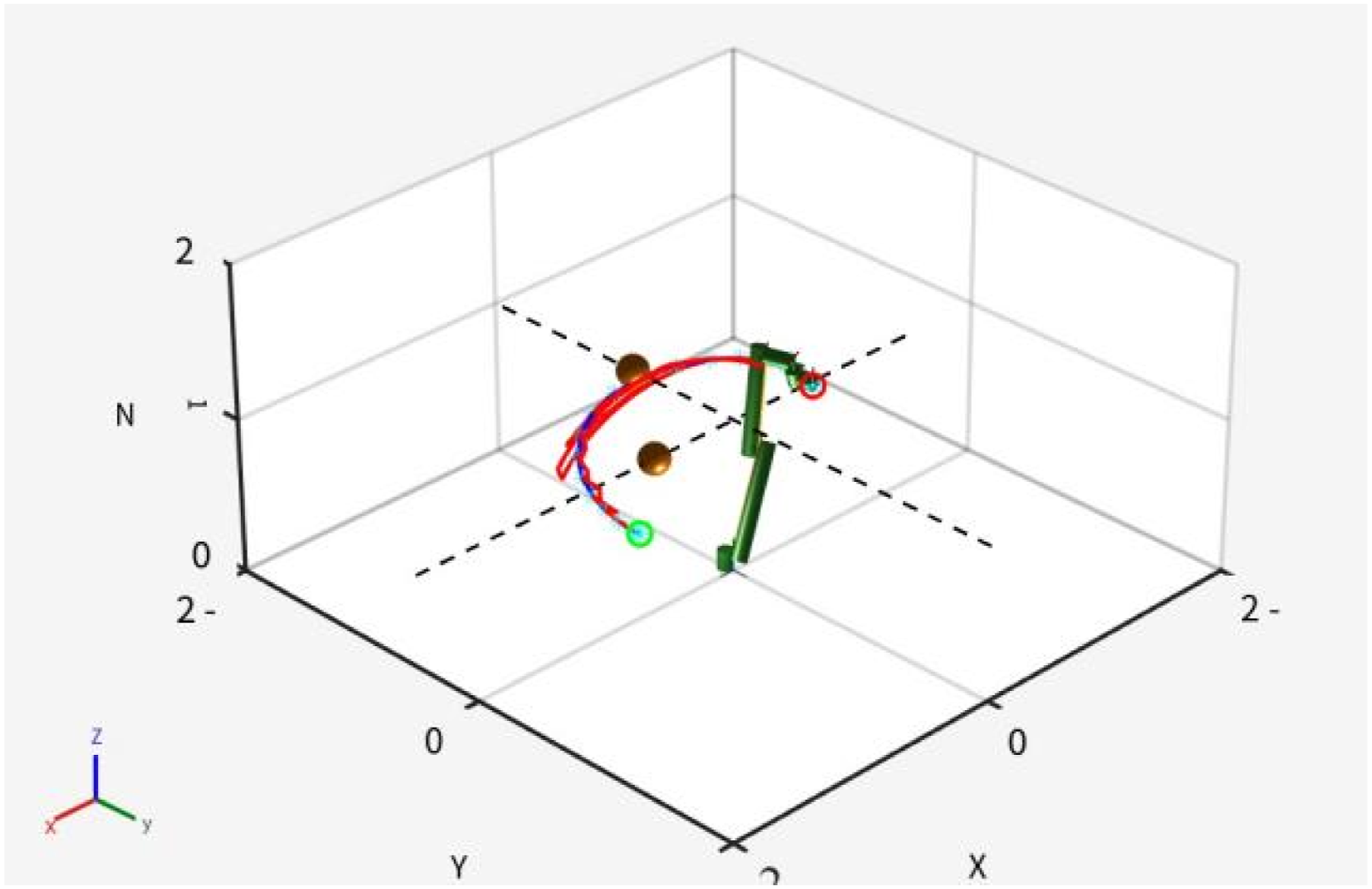
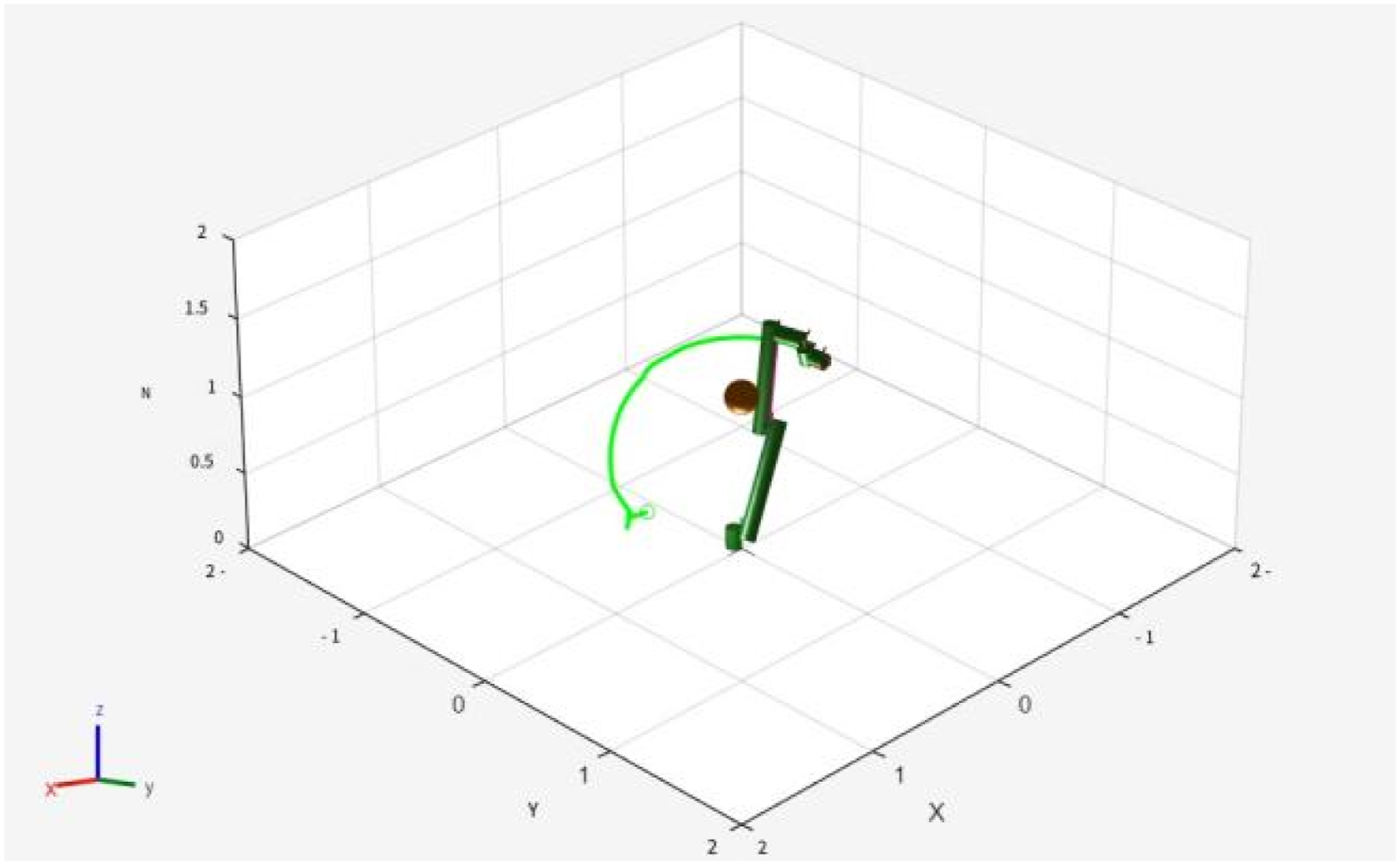
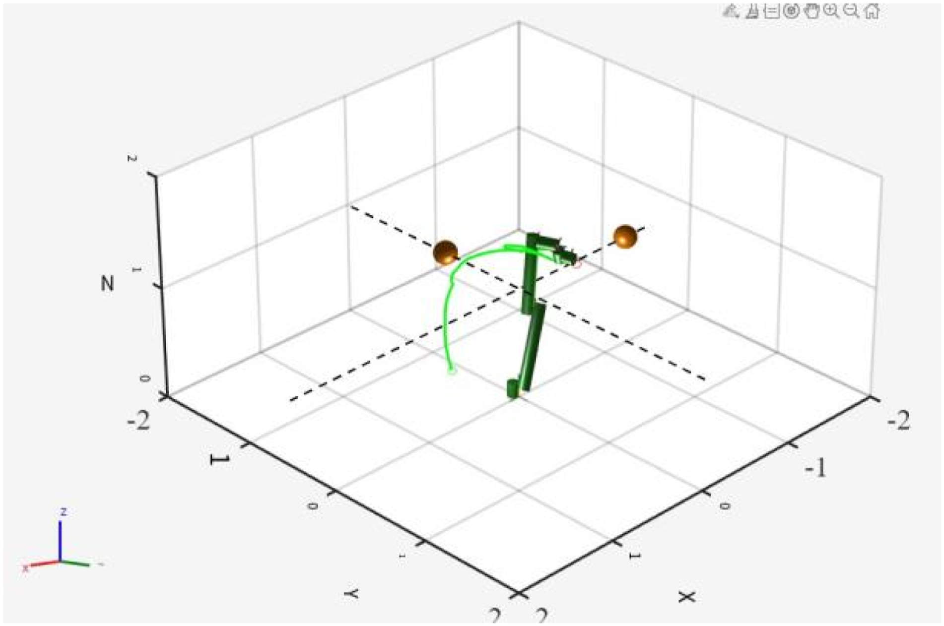
Three obstacles are set up in the working space of the robotic arm, of which obstacle 1 is a static obstacle, and obstacle 2 and obstacle 3 are dynamic obstacles with uniform speed. As shown in Figure 29 is the movement path of the robotic arm in the uniform velocity obstacle environment, the radius of the three obstacles are 0.1m, the center position of obstacle 1 is (0, 0, 0.7); the starting position of obstacle 2 is (0, 0, 1), and along the Y-axis to do the reciprocating motion at a speed of 0.8m/s, the activity interval on the Y-axis is [-2, 2]; the starting position of obstacle 3 is (1,- 0.25, 0.6), and reciprocating motion along the X-axis with a speed of 0.5m/s, and the activity interval on the X-axis is [-2, 2]. Figure 30 shows the distance from the end-effector to the target point of the robotic arm during the avoidance of a uniform obstacle.

Figure 29.

Robotic arm path planning under uniform obstacles.

Figure 30.

Distance from end-effector to target point.

Figure 30 shows that the entire robotic arm obstacle avoidance movement is divided into three stages, the first stage of the robotic arm is not affected by the dynamic obstacles gradually moving toward the target point; in the second stage, as the dynamic obstacle gradually approaches the robotic arm, the repulsive force on the robotic arm will increase, “pushing” the robotic arm away from the obstacle, causing the distance between the end effector of the robotic arm and the target point to become farther and farther; in the third stage, the obstacle is gradually far away from the robotic arm, and the repulsive force on the robotic arm from the dynamic obstacle will be smaller and smaller, and then it will gradually move towards the target point again.

The operation status of the robotic arm can be observed through changes in the angle and angular velocity of each joint of the robotic arm, and Figure 31shows the trajectory change of each joint of the robotic arm during the process of avoiding the uniform obstacle. From the Figure 31, it can be seen that in order to avoid dynamic obstacles, the joint angle change fluctuates so that each linkage of the robotic arm can avoid the obstacles.

Figure 31.

Operation status of each joint of the robotic arm under obstacles of uniform motion.

It can be seen from the results of experiment 1 that the path of the end-effector is smooth and there are no too many inflection points in the whole process of avoiding the obstacles moving at uniform speed. Moreover, the trajectory of each joint is relatively stable, which will not cause frequent jitter in the process of moving the robot arm.

Dynamic obstacle avoidance experiment II

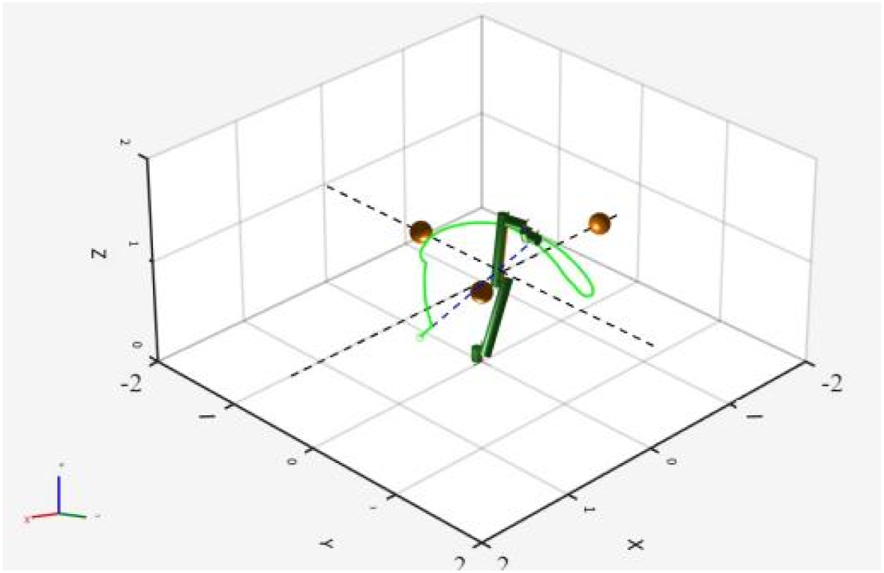
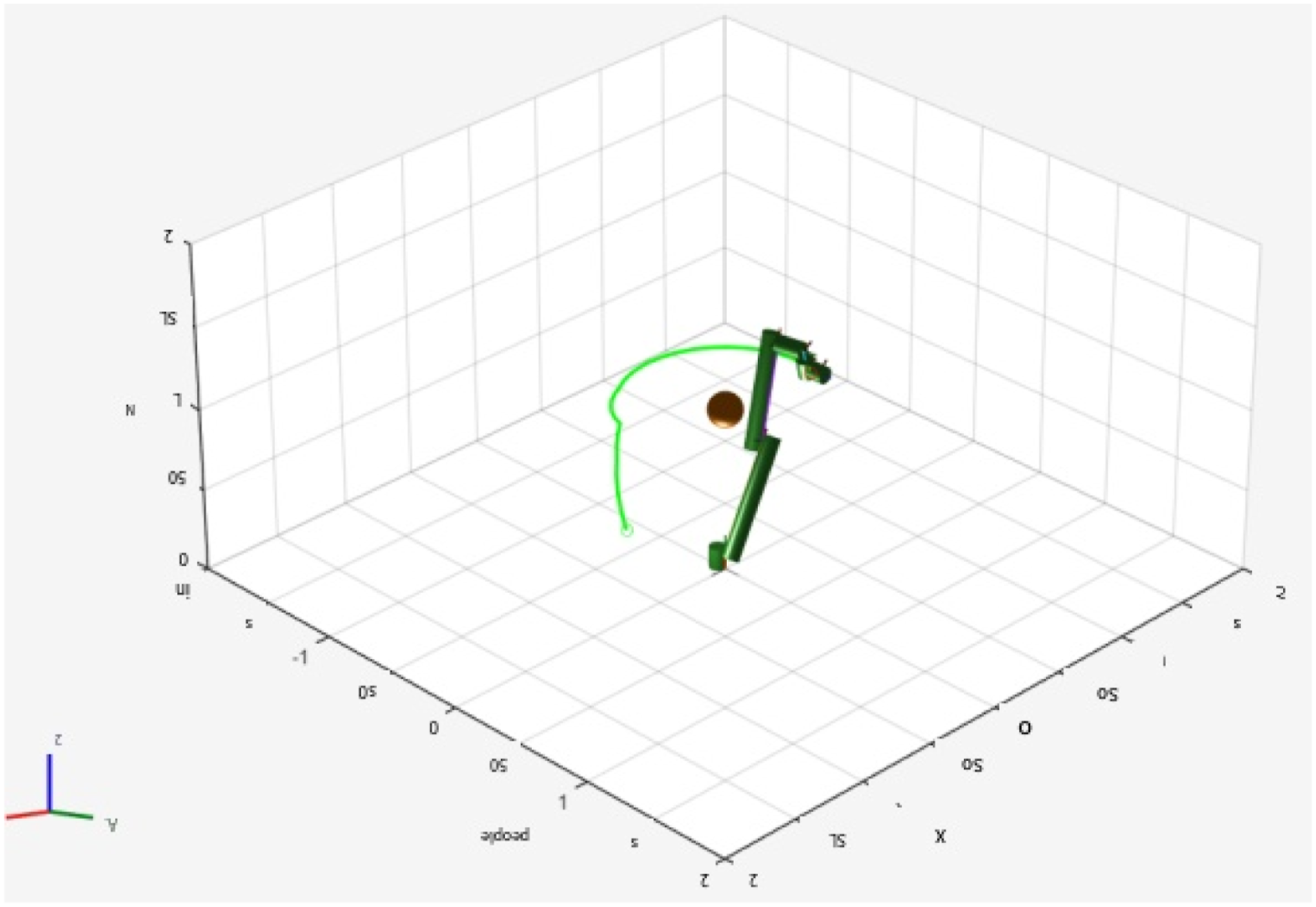
In order to further verify the effect of this paper’s algorithm on obstacle avoidance in dynamic environments, variable-speed motion obstacles are added to the working space of the robotic arm. Set two variable-speed obstacles with a radius of 0.1m, the starting position of obstacle 1 is (0, 0, 1), let the obstacle 1 reciprocate along the Y-axis; the starting position of obstacle 2 is (1, -0.5, 0.6), let the obstacle 2 reciprocate along the X-axis, and set the obstacle speed change formula as v = cos (t/50) m/s. Figure 32 shows the path planning of the robot arm when avoiding obstacles in variable speed motion. Figure 33 shows the distance between the end-effector and the target point in the process of avoiding variable-speed obstacles.

Figure 32.

Robotic arm path planning under variable speed obstacles.

Figure 33.

Distance between end-effector and target point under avoiding obstacles in variable speed movement.

In Figure 33, P1 to P2 is the obstacle-avoidance path planning when the robotic arm encounters obstacle 2 in the process of operation, the end-effector is getting closer and closer to the end point under the action of the repulsive force field of obstacle 2. P2 to P3 is the obstacle-avoidance path planning when obstacle 2 is gradually far away from the robotic arm and obstacle 1 is close to the end point, in the middle of which the end-effector is getting further and further from the end point. After P3, obstacle 1 gradually moves away, and the repulsion force on the robotic arm decreases, gradually moving towards the endpoint. Figure 34 shows the operation diagram of each joint under obstacle avoidance variable speed obstacle.

Figure 34.

Operation status of each joint of the robotic arm under variable speed movement obstacles.

From Figure 34, it can be seen that between 2.7s and 3.9s, because of the action of obstacle 2, the value of joint angle 2 gradually increases to keep the whole the robotic arm away from the obstacle, and between 3.9s and 5.4s, under the joint action of obstacle 1 and obstacle 2, the value of joint angle 2 and joint angle 3 gradually decreases in order to achieve the effect of obstacle avoidance.

The ability of a robot to avoid dynamic obstacles mainly depends on its distance from the obstacle. Regardless of whether the movement speed of obstacles changes or the movement trajectory changes, the closer the obstacle is to the robot and the faster the speed, the greater the repulsive force the robot experiences and the faster the change, causing the robot to move away from the obstacle. Therefore, although the algorithm proposed in this paper is still applicable to obstacles with constantly changing movements.

Simulation scene setup for verification

To further verify the performance of the path planning algorithm proposed in this paper, static obstacle and dynamic obstacle scenarios were designed and built based on the MIoT.VC platform for simulation verification, and the final results were analyzed.

Based on the MIoT.VC host computer control system

In practical applications, MIoT.VC can not only simulate and analyze the production process, but also communicate with the field equipment as a host computer to control the operation of the field equipment. As shown in Figure 35, it is the upper computer control system based on MIoT.VC.

Figure 35.

Upper computer control system based on MIoT.VC.

Vision module

The Kinect camera is a 3D vision camera whose body contains a color camera, an infrared camera and an infrared emitter. The Kinect camera has depth perception capabilities and requires calibration of the camera’s internal and external parameters before use (Figure 36).

Figure 36.

Hand-eye calibration.

The internal parameters of the Kinect camera are calibrated at the factory, and the external parameters can be calibrated by the “eye-out-of-hand” calibration method.

Host computer

As the upper computer, MIoT.VC mainly accomplishes functions such as robotic arm modeling, environmental modeling, path planning and trajectory planning. In addition, MIoT.VC can debug PLC code in a virtual environment and supports direct connection to mainstream brand PLCS, Hmis, SCADA and other devices via communication protocols such as OPC-UA and SiemensS7-PLC for data interaction with field devices, Read mode, subscribe mode and write mode can be used for data points of the field PLC controller.

Communication module

Modbus is a commonly used communication protocol in the industrial field and is also a master/slave architecture protocol. In the same network, only one device can be the master device, and all other devices are slave devices. The master device is responsible for sending request commands to the slave devices, and the slave devices respond to the master device after receiving the commands. Through the Modbus protocol, the MIoT.VC platform can act as the master device, that is, the Modbus client, and the robotic arm controller as the slave device, that is, the Modbus server.

The communication model between the client and the server is shown in the Figure 37, and the communication process between the two is as follows:

(1) The client initiates the connection request, and then the server receives the request to complete the TCP connection between the MIoT.VC platform and the robotic arm.

(2) The client sends the request data packet.

(3) The server receives the data packet, processes the data and sends the response data packet to the client.

(4) After receiving the data packet, the client parses the data and processes it accordingly.

Figure 37.

Figure modbus communication model.

During the movement of the robotic arm, sensors on the robotic arm transmit data such as joint angles and end effector coordinates to the controller, which then sends these data to the client via the Modbus protocol to drive the movement of the virtual model of the robotic arm on the client. Likewise, for the instructions issued by the client, the Modbus protocol is used to send the instructions to the controller, which converts the instructions into drive signals to make the robotic arm move.

Motion control module

The core components of a robotic arm’s motion control module include controllers, servo drives, and motors for each joint. The upper computer software is responsible for converting various motion instructions into angular variations of each joint. Then the controller further converts these Angle changes into corresponding joint pulse instructions. When the servo driver receives these pulse instructions, it will allocate them reasonably and amplify the current and voltage according to the configuration, thereby driving the motor at each joint to move, ultimately achieving the rotation function of each joint of the robotic arm. At the same time, the controller and servo driver of the robotic arm also receive feedback information on angles and speeds from the joints to achieve precise motion control.

Scenario simulation experiment

Simple scenarios

Select the “UR10” robotic arm under “Universal Robots” in MIoT.VC’s component library and set its position coordinates in space to (0,0,0). Set two static obstacles. Obstacle 1 is a blue spherical obstacle with a radius of 150mm and coordinates of (0,0,900), and obstacle 2 is a yellow spherical obstacle with a radius of 100mm and coordinates of (250, 250, 1000). Set the initial attitude for mechanical arm [28.65 ° and 145.63 ° and 8.59 ° and 1.15 ° and 13.75 ° and 28.07 °], target attitude for [170.17 ° and 119.84 ° and 20.05 ° and 58.44 ° and 8.02 ° and 28.07 °]. As shown in the Figure 38.

Figure 38.

3D static environment simulation scene.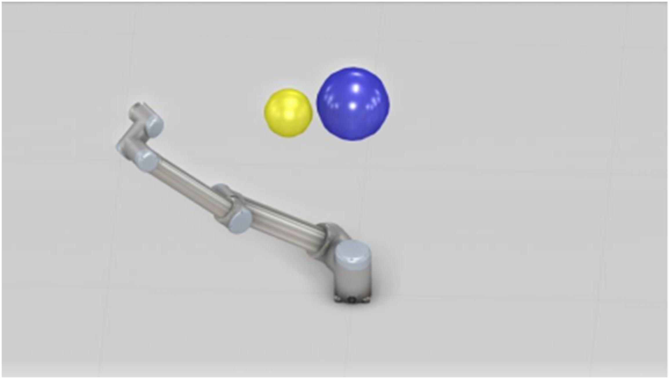

The static obstacle avoidance path planning is carried out respectively by using the traditional Bi-RRT algorithm and the improved APF-Bi-RRT algorithm proposed in this paper. Figure 38 shows the path planning results of the traditional Bi-RRT algorithm, and Figure 40 shows the path planning results of the improved APF-Bi-RRT algorithm. The average of 50 experiments of the two algorithms is recorded in Table 6.

Table 6.

Comparison of path planning results between Bi-RRT algorithm and improved APF-Bi-RRT algorithm1.

Algorithm name	Average distance
Bi-RRT Algorithm	3.84
Improvement APF-Bi-RRT Algorithm	2.55

Bi-RRT Algorithm and Improvement APF-Bi-RRT Algorithm Comparison of Path Planning Results.

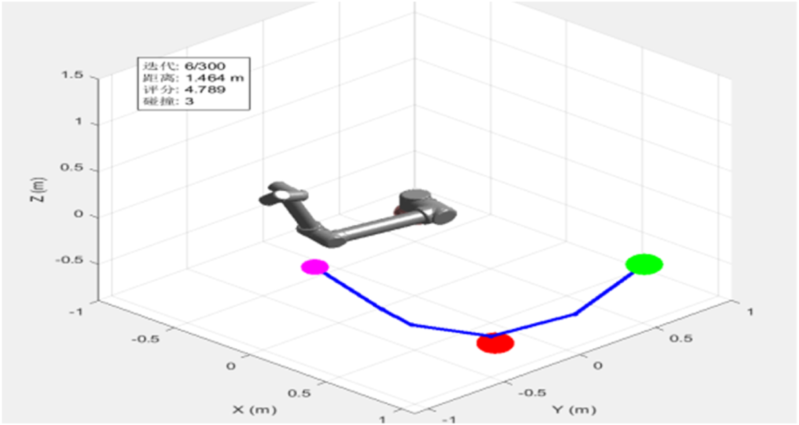
By comparing the path planning results in Figure 39 and Figure 40, it can be intuitively seen that the path distance planned by the improved APF-Bi-RRT algorithm is shorter than that planned by the Bi-RRT algorithm, and the path is smoother with fewer inflection points, reducing the jitter of the robotic arm due to the unsmooth path. After multiple experiments, the results in Table 6 show that the improved APF-Bi-RRT algorithm can shorten the path distance by approximately 33.6% compared to the Bi-RRT algorithm.

Figure 39.

Static path planning based on Bi-RRT algorithm.

Figure 40.

Static path planning based on an improved APF-Bi-RRT algorithm.

Material handling scenarios between conveyor belts

To further validate the performance of the path planning algorithm proposed in this paper, the motion state of the robotic arm was observed by building a typical conveyor belt robotic arm material handling scenario, as shown in Figure 41and Conveyor Belt 2 are sensor-equipped conveyor belts. When the sensor on conveyor belt 1 detects the material, conveyor Belt 1 stops moving and the mechanical arm moves the material onto conveyor belt 2, and the sensor on conveyor belt 2 detects the material and then starts transporting.

Figure 41.

The scene of material handling between conveyor belts.

The material handling path of the robotic arm was planned using the improved APF-Bi-RRT algorithm, and the planning results are shown in Figure 42. After grasping the material, the robotic arm first moves to transition point 1 to prepare for the next stage of movement; Secondly, to ensure that the material is placed accurately, transition point 2 is set at a certain distance directly above the placement position. Move from transition point 1 to transition point 2. It can be seen from the figure that the path planned between the two points is a smooth curve without any extra nodes, once again verifying the superiority of the path planning algorithm proposed in this paper; Finally, transition point 2 is placed onto the conveyor belt. Observe the movement state of the robotic arm, the smooth path trajectory, and the stability of the robotic arm’s handling process by building a typical robotic arm material handling scenario between conveyor belts.

Figure 42.

Path planning results for robotic arm material handling between conveyor belts.

Dynamic scene simulation experiment

Collaborative robotic arms are often used in human-machine collaboration scenarios, mostly assisting people in moving workpieces or working together with people to complete tasks such as assembling products, and thus face dynamic obstacles such as workers or moving workpieces. To verify that the path planning algorithm in this paper can help the robotic arm avoid dynamic obstacles, a human-machine collaboration working scenario was built in MIoT.VC to conduct a simulation experiment on the dynamic obstacle avoidance of the robotic arm. Figure 43 is a three-dimensional dynamic environment simulation scene. First, set the position coordinates of the robotic arm to (0,0,800), and the size of the worktable (length × width × height) to 1000mm×500mm×760mm. On the left side of the worktable is the sensor-equipped conveyor belt. When the part reaches the designated position, the conveyor belt stops moving and the robotic arm lifts the part onto the worktable to the right of the worker. During this process, the worker is set to process the workpiece, which is a cylindrical workpiece with a radius of 75mm and a height of 150mm.

Figure 43.

Three-dimensional dynamic environment simulation scene.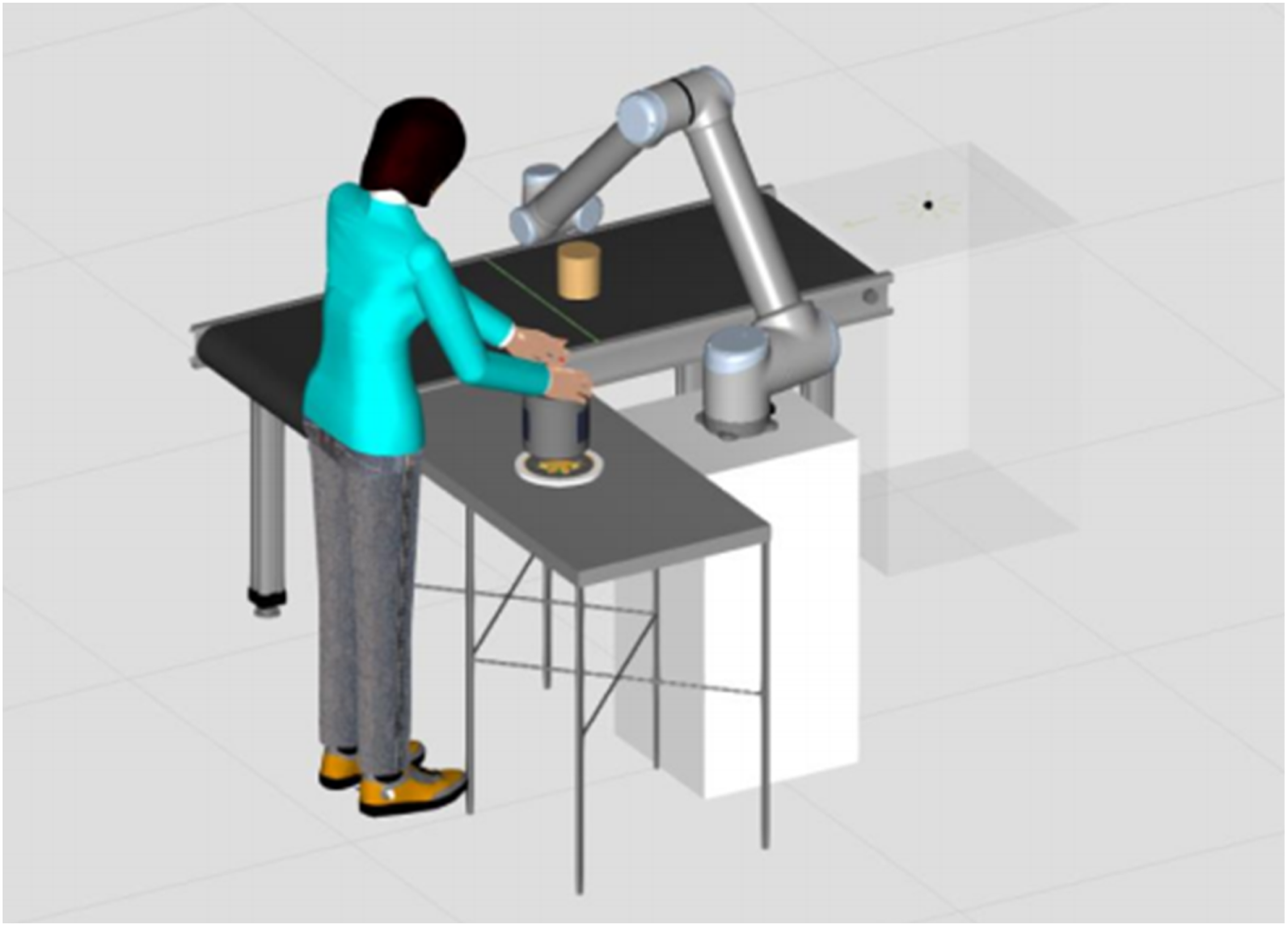

In dynamic obstacle avoidance simulation, the improved APF-Bi-RRT algorithm proposed in this paper is applied in MIoT.VC to enable the robotic arm to avoid moving workpieces. Figure 44 shows the path planning of the UR10 robotic arm for dynamic obstacle avoidance while the worker is processing the workpiece. In Figure 44 (a) is the initial pose of the robotic arm when grasping the part, (a) to (b) is the pose of the robotic arm when it needs to move the part up a certain distance after grasping to facilitate subsequent handling, and (c) is the pose of the robotic arm when it is not affected by moving obstacles during the handling process; From (d) - (e), it can be seen that the robotic arm is affected by the moving workpiece, and the end gradually moves away from the obstacle. This is because, under the effect of the improved APF-Bi-RRT algorithm, the repulsive field generated by the moving obstacle pushes the joints of the robotic arm away, and as the obstacle gets closer, the repulsive force generated by the repulsive field becomes greater; From (f) to (g), the distance between the moving workpiece and the robotic arm gradually increases, at which point the repulsive force decreases and the gravitational force increases, and the robotic arm begins to move in the direction of the target position; (h) - (i) is the process by which the robotic arm lowers the part.

Figure 44.

Dynamic obstacle avoidance path planning for robotic arms in human-machine collaboration scenarios.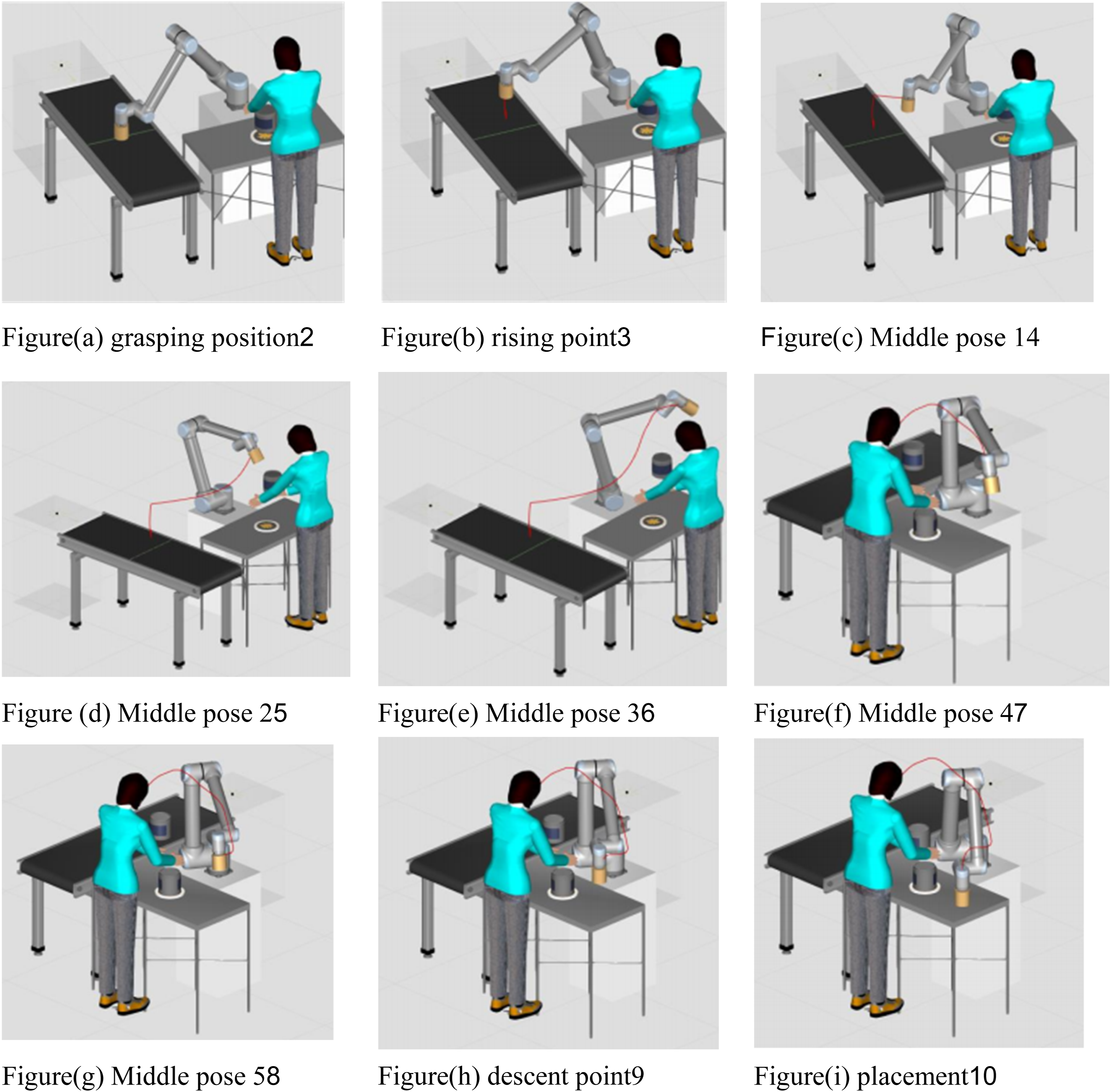

The trajectory planning of the robotic arm is then carried out. Since the trajectory changes between the grasping position and the ascending point and from the descending point to the placement position are very small and take very short time, it will not significantly affect the final result. Therefore, this paper only discusses the trajectory planning of the robotic arm from the ascending point to the descending point. The working time of the robotic arm was reduced from 10 seconds to 5.92 seconds, and the efficiency was increased by 40.8%.

By setting up different scenarios for simulation verification, it was demonstrated that the improvement of the algorithm enhanced the efficiency of the robotic arm and optimized the working path of the robotic arm.

Conclusion

An improved APF-Bi-RRT algorithm is proposed for path planning of collaborative robot under dynamic obstacles.

(1) Use the cost function to select the nodes on the path derived by the Bi-RRT algorithm and eliminate the redundant nodes; The gravitational and repulsive fields of the APF algorithm were reconstructed, and the improved Bi-RRT algorithm was used to solve the problem of the APF algorithm getting stuck in local minima; The combination of the two algorithms not only enables the robotic arm to achieve dynamic obstacle avoidance, but also makes the path of the end effector smoother and the operation of the joint smoother throughout the obstacle avoidance process. The effectiveness of the algorithm was verified through simulation experiments of collaborative robot path planning in different dynamic types of obstacle environments.

(2) Compare the algorithms by using multiple algorithms (APF, RRT*, RRT-Connect, PRM, Bi-RRT) for path planning of robotic arms in the same environment, and compare the advantages and disadvantages of the algorithms as well as the path data to confirm the applicability of the algorithms and the excellence of the improvements.

(3) Build obstacle avoidance path planning for the robotic arm in different simulation scenarios on the simulation platform, verify the path planning of the robotic arm in different real environments, and prove that the improvement of the algorithm has enhanced the working efficiency of the robotic arm and optimized its working path.

The method proposed in this paper is also applicable to the material handling of robotic arms in complex storage environments, which not only enables the robotic arms to dynamically avoid obstacles and improve safety, but also makes them run smoothly, reduces wear and tear, and achieves a low-carbon effect.

Footnotes

ORCID iD

Yufei Li

Funding

The authors disclosed receipt of the following financial support for the research, authorship, and/or publication of this article: Project Category: Technology Innovation Guidance Program (Fund) - Qin Chuangyuan’s “Scientists+Engineers” Team Construction; Project Number: 2025QCY-KXJ-048.

Declaration of conflicting interests

The authors declared no potential conflicts of interest with respect to the research, authorship, and/or publication of this article.

References

Keshvarparast

Battini

Battaia

, et al. Collaborative robots in manufacturing and assembly systems: literature review and future research agenda. Journal of Intelligent Manufacturing 2024; 35(5): 2065–2118. https://doi.org/10.1007/s10845-023-02137-w

Waga

Benhlima

Bekri

, et al. Waypoint-guided trajectory planning for mobile robots using GPT-4.1 mini and ensemble learning-based action prediction. Array 2026; 29: 100636–100636. https://doi.org/10.1016/j.array.2025.100636

Liu

Ding

Zou

, et al. Multirobot conflict coordination and dynamic obstacle avoidance cooperative path planning. Intelligent Service Robotics 2025; 18(3): 1–20. https://doi.org/10.1007/s11370-025-00595-0

Katona

Neamah

Korondi

. Obstacle Avoidance and Path Planning Methods for Autonomous Navigation of Mobile Robot. Sensors 2024; 24(11): 3573. https://doi.org/10.3390/s24113573

Meng

Fang

. A UGV Path Planning Algorithm Based on Improved A* with Improved Artificial Potential Field. Electronics 2024; 13(5): 972. https://doi.org/10.3390/electronics13050972

Xia

Sang

, et al. Path Planning for Obstacle Avoidance of Robot Arm Based on Improved Potential Field Method. Sensors (Basel, Switzerland) 2023; 23(7): 3754. https://doi.org/10.3390/s23073754

Yuan

Shuai

Zhang

. A Dynamic Multiple-Query RRT Planning Algorithm for Manipulator Obstacle Avoidance. Applied Sciences 2023; 13(6): 3394. https://doi.org/10.3390/app13063394

Song

. Manipulator Motion Planning Based on Improved RRT Algorithm. Journal of Physics: Conference Series 2023; 2456(1): 012008. https://doi.org/10.1088/1742-6596/2456/1/012008

Yang

Luo

Duan

, et al. Research on multi-objective point path planning for mobile inspection robot based on Multi-Informed-Rapidly Exploring Random Tree*. Engineering Applications of Artificial Intelligence 2025; 151: 110645–110645. https://doi.org/10.1016/j.engappai.2025.110645

10.

Wang

Jiang

Luo

, et al. Path planning of a 6-DOF measuring robot with a direction guidance RRT method. Expert Systems With Applications 2024; 238(PD): 122057. https://doi.org/10.1016/j.eswa.2023.122057

11.

. Machine Tool Assisted Robot Control Method Based on RRT Algorithm. Journal of The Institution of Engineers (India): Series C 2025; 106(prepublish): 1–13. https://doi.org/10.1007/S40032-025-01269-7

12.

Kozhubaev

Yang

. Simulation of Dynamic Path Planning of Symmetrical Trajectory of Mobile Robots Based on Improved A* and Artificial Potential Field Fusion for Natural Resource Exploration. Symmetry 2024; 16(7): 801. https://doi.org/10.3390/sym16070801

13.

Qin

Chen

. Three-Dimensional Path Planning for Mobile Robots Based on Hybrid Strategy and Artificial Potential Field Methods. Signal, Image and Video Processing 2025; 19(13): 1076. https://doi.org/10.1007/s11760-025-04647-x

14.

Chen

Ding

, et al. Research on Real-Time Obstacle Avoidance Motion Planning of Industrial Robotic Arm Based on Artificial Potential Field Method in Joint Space. Applied Sciences 2023; 13(12): 6973. https://doi.org/10.3390/app13126973

15.

Lin

Shao

. Path planning of mobile robot based on improved PRM and APF. Measurement and Control 2025; 58(8): 979–995. https://doi.org/10.1177/00202940241291282

16.

Zhang

Long

, et al. A Multi-Policy Rapidly-Exploring Random Tree Based Mobile Robot Controller for Safe Path Planning in Human-Shared Environments. Sensors 2025; 25(22): 7008. https://doi.org/10.3390/s25227008

17.

Yang

Guo

Liu

, et al. Research on APF-Bi-RRT Algorithm of Adaptive Step Strategy for Robot Path Planning. Arabian Journal for Science and Engineering 2024; 50(17): 1–14. https://doi.org/10.1007/s13369-024-09642-x

18.

Daohua

Lisheng

Guanling

, et al. APF-IRRT*: An Improved Informed Rapidly-Exploring Random Trees-Star Algorithm by Introducing Artificial Potential Field Method for Mobile Robot Path Planning. Applied Sciences 2022; 12(21): 10905.

19.

Liwei

Lixia

Ping

, et al. An Effective Dynamic Path Planning Approach for Mobile Robots Based on Ant Colony Fusion Dynamic Windows. Machines 2022; 10(1): 50.

20.

Liu

Xiong

, et al. Path Planning for Mobile Robots Based on the Improved DAPF-QRRT* Strategy. Electronics 2024; 13(21): 4233. https://doi.org/10.3390/electronics13214233

21.

Wang

Zhang

Chen

, et al. Research on single-target point navigation task of indoor mobile robot integrating RRT-Connect and DWA algorithms. Journal of Central South University(Science and Technology) 2023; 54(11): 4326–4337.

22.

Xiong

Hou

Wang

, et al. Classified-RRT*: Node classification RRT*-based algorithm with improved solution performance and convergence rate. Expert Systems With Applications 2026; 296(PC): 129118. https://doi.org/10.1016/j.eswa.2025.129118

23.

Chandrasekar

Gnanasekar

. A dual quaternion approach to kinematic modeling and evaluation of PRR-type robotic manipulators. Progress in Engineering Science 2025; 2(4): 100174. https://doi.org/10.1016/j.pes.2025.100174

24.

Long

Zhang

, et al. Human-Risk-Aware Safe Path Planning Based on Reinforcement Learning for Autonomous Mobile Robots. Sensors 2025; 25(23): 7211. https://doi.org/10.3390/s25237211