Sage Journals: Discover world-class research

Abstract

In recent years, there has been growing interest in the prediction of financial market trends, due to its potential applications in the real world. Unlike traditional investment avenues such as the stock market, the foreign exchange (Forex) market revolves around two primary types of orders that correspond with the market's direction: upward and downward. Consequently, forecasting the behaviour of the Forex behaviour market can be simplified into a binary classification problem to streamline its complexity. Despite the significant enhancements and improvements in performance seen in recent proposed predictive models for the forex market, driven by the advancement of deep learning in various domains, it remains imperative to approach these models with careful consideration of best practices and real-world applications. Currently, only a limited number of papers have been dedicated to this area. This article aims to bridge this gap by proposing a practical implementation of deep learning-based predictive models that perform well for real-world trading activities. These predictive mechanisms can help traders in minimising budget losses and anticipate future risks. Furthermore, the paper emphasises the importance of focussing on return profit as the evaluation metric, rather than accuracy. Extensive experimental studies conducted on realistic Yahoo Finance data sets validate the effectiveness of our implemented prediction mechanisms. Furthermore, empirical evidence suggests that employing the use of three-value labels yields superior accuracy performance compared to traditional two-value labels, as it helps reduce the number of orders placed.

Keywords

Financial forecasting model financial time series stock-movement forecasting forex market return profit

Introduction

In the realm of time-series data analysis and prediction, numerous studies have delved into uncovering valuable insights from data. Time-series analysis finds wide application in various financial market scenarios, with Forex being a prime example of such data. This topic remains of great interest for investors and researchers alike, not only due to its practical implications in financial activities, but also due to the persisting challenges within this research domain.^1,2 The primary objective of time-series data prediction is to forecast continuous values for future periods. Recent years have witnessed the emergence of powerful prediction showing algorithms that have shown effectiveness across diverse time series time series datasets.³ However, financial data presents unique challenges due to their susceptibility to multiple factors that influence them. Numerous articles have highlighted the primary challenge of financial data: its data: its inherent randomness and volatility. Given these challenging characteristics, it is considered difficult to analyse financial data comprehensively and to make accurate predictions is considered difficult. Consequently, several studies have changed the focus towards predicting market trends rather than specific values, defining the task as a classification problem.^1,4–6 This approach has gained traction due to its perceived efficacy in mitigating price fluctuations. In formulating forex forecasting as a classification task, recent studies focus on training and evaluating models based on categorisation accuracy. However, the pursuit of improving trend classifiers based solely on accuracy may not necessarily translate into increased profitability.^7,8 Our extensive experiments reveal that the accuracy of a predictive model does not exhibit a linear correlation with profitability. Despite many studies emphasising high accuracy as a performance metric, it does not guarantee profitability in real-world trading scenarios. Therefore, implementing when implementing financial market prediction algorithms,⁹ prioritising profitability as the optimisation factor becomes crucial. Investors should regard predictive models as indicators, supplementing them with external information such as news and additional indicators for decision making. Relying solely on these models for trading decisions may not yield the desired results. Thus, understanding the limitations and considering various factors beyond the accuracy is essential for the practical implementation of financial prediction algorithms.

The prediction of Forex (foreign exchange) has been a significant area of research due to the substantial impact of exchange rates on international trade, investment and economic policy. The literature on forex prediction encompasses various methodologies, including statistical models, machine learning algorithms and advanced technique approaches.

Statistical models like ARIMA (autoregressive integrated moving average) and GARCH (generalised autoregressive conditional heteroskedasticity) are traditional approaches for Forex prediction. ARIMA models are effective in modelling linear dependencies in time series data, but struggle with nonlinear patterns and require extensive parameter tuning. GARCH models are used to predict volatility and are effective for time-varying volatility, but may not predict price direction accurately. ARIMA models have been widely used for Forex prediction due to their ability to model linear dependencies in time-series data. However, they have limitations in capturing nonlinear patterns and are sensitive to parameter tuning. GARCH models are used to predict volatility in Forex markets. They are effective in modelling time-varying volatility, but may struggle predicting the actual price direction. Furthermore, simple and multiple linear regression models have been applied to forex prediction. HortaHorta and Mora-Valencia¹⁰ address this problem by appropriately calculating uncertainties in time series forecasting using Bayesian deep learning. Their research highlights that conventional neural networks are typically uncalibrated, which can affect the reliability of forecasts. For example, in financial markets, where precise predictions are vital, uncalibrated models may provide overconfident or underconfident predictions, leading to suboptimal decision making. The work of Héctor J. Horta and Andrés Mora-Valencia¹¹ on ‘Forecasting VIX using Bayesian Deep Learning’ provide valuable insights into addressing this challenge. By incorporating Bayesian methods, their approach allows for better uncertainty estimation, enhancing the reliability of forecasts. This method not only improves the predictive performance, but also provides a measure of confidence in the predictions, which is essential for making informed decisions in high-stakes environments like finance. Although easy to implement and interpret, they often fail to capture the non-linear complex and non-linear relationships present in the Forex market. In addition, logistic regression models are used for binary classification problems in forex prediction, such as predicting whether the exchange rate will go up or down. These models are limited by their linear nature.

Machine learning algorithms,¹² such as support vector machines (SVM), artificial neural networks (ANN) and ensemble methods such as random forests, such as random forests, have shown promise in the prediction of forex. SVMs perform well in high-dimensional spaces, but can be computationally intensive. ANNs, including feedforward and recurrent neural networks, can capture nonlinear patterns but require large datasets and substantial computational power. Ensemble methods like random forests handle high-dimensional data effectively, but can be prone to overfitting. Clustering algorithms are frequently used today. ANNs,¹² including feedforward and recurrent neural networks, have shown promise in capturing nonlinear patterns in Forex data. However, they require a large amount of data and computational power. SVMs¹³ are used for classification and regression tasks in Forex prediction. They perform well in high-dimensional spaces, but can be computationally intensive. Ensemble methods such as random forests are effective in handling high-dimensional data and in capturing complex interactions between variables. They provide good accuracy but can be prone to overfitting. Techniques like K-means and hierarchical clustering are used to identify patterns and group similar instances in Forex data. These methods are helpful for exploratory data analysis but not directly for prediction.

Recent advances in deep learning have led to the use of long-short-term memory (LSTM) networks and convolutional neural networks (CNNs) for forex prediction. LSTMs are particularly effective for time series prediction, because of their ability to capture long-term dependencies. Studies by Yan et al.¹⁴ and others have shown LSTM's superior performance in financial time series prediction, although with significant computational resource requirements. CNNs, adapted for time series by treating data as images, excel in feature extraction, but are less common compared to LSTMs. Our work builds on these methodologies by proposing a deep learning-based predictive model focussing on practical implementation and real-world trading activities. Unlike previous studies that emphasise precision, our research prioritises return profit as the evaluation metric, aligning model performance with real-world financial goals.

While many studies focus on accuracy as a performance metric, our research highlights the non-linear relationship between accuracy and profitability. For example, our experiments show that a model with high accuracy does not necessarily yield higher profits in real trading scenarios. In addition, we introduce a three-value labelling system based on market states, which has been shown to reduce the number of orders placed and improve prediction accuracy compared to traditional binary labelling. This approach aligns with the findings of Zhao et al.,¹⁵ who also suggested a multi-threshold labelling system for better market trends. Finally, our study emphasises practical implementation using realistic Yahoo Finance datasets and Metatrader5 platform data. This practical focus is a significant addition to the literature, providing actionable information for traders and investors. The paper is structured into five sections. In section ‘Related work’, existing methods are discussed, highlighting the challenges that hinder their implementation. Section ‘Background knowledge’ provides essential background knowledge before introducing our proposed methods in the subsequent following section. Our implementation methods are detailed in section ‘Proposed methods’, including the calculation of profit for evaluation and the three-value labelling approach for categorising market states. Section ‘Experimental results’ presents the data and experimental results, demonstrating the nonlinear relationship between accuracy and earning profit, along with the effectiveness of our implementation methods. Finally, section ‘Conclusion’ concludes the paper, offering suggestions for future improvements.

Related work

Financial prediction is an intriguing research avenue, with numerous studies dedicated to tackling this challenge and producing noteworthy results. Depending on the problem formulation and prediction objectives, financial prediction can generally be categorised into two main approaches: price prediction (in section ‘Price prediction approach’) and trend classification (in section ‘Trend classification approach’).

Price prediction approach

Price prediction poses a significant challenge akin to time-series data prediction, where the LSTM network stands out as a cutting-edge technique for handling sequential data and addressing multiple task-driven learning objectives. Although not considered a challenging approach to financial data,^11–13 architectures based on LSTM are often considered the most suitable to solve this problem. However, several studies have demonstrated the effectiveness of LSTM networks when applied in various ways. For example, in studies by Yan et al.,¹⁴ stock data undergo preprocessing before being input into LSTM networks for predictions, showcasing effectiveness when combined with various data processing methods. In their work, Yan et al.,¹⁴ proposed an integrated approach called the firefly algorithm modified support vector regression (SVR) modified (SVR-MFA), applied for stock price prediction. The SVR-MFA model uses MFA to enhance global convergence, employing dynamic adjustment and opposition-based chaotic strategies. It optimises SVR's hyperparameters to enhance prediction accuracy. In recent years, various machine learning techniques and artificial neural networks (ANNs), including LSTM and CNNs, have gained traction in stock price predictions. These ANN-based architectures excel at uncovering hidden features through self-learning processes. They serve as excellent approximators, capable of discerning latent relationships within vast and intricate datasets, making them suitable for handling nonlinear, highly dynamic time-series datasets such as stocks and forex. Several studies,^16,17 demonstrate the synergistic combination of ANN and Random Forest (RF) to predict stock closing prices, with efficiency improvements ranging from 60% to 86% compared to previous methods.

Trend classification approach

In addition to price prediction, the classification of financial trends represents another significant approach in this domain, which is the main focus of our study in this paper. In particular, recent research has shown a high level of interest in this area. For example, Chen et al. have introduced an improved graph convolutional network (IGCN) designed to capture stock features based on topological structure data, which is then integrated with the CNN to predict stock trends.¹⁸ Similarly, Yin et al. have employed the exponential smoothing method to preprocess initial data and calculate relevant technical indicators, which are then utilised and used as features for selection. These selected characteristics are subsequently inputted into a random forest (RF)-based the RF model for stock trend classification. In particular, in addition to the characteristics derived from historical data, news plays a significant role in market activity. Consequently, various approaches have emerged for the prediction of stock trends based on financial news platforms and social networks.^19,20 For example, Chen et al. incorporated Chinese news and technical indicators into their study to predict stock trends.²¹ Furthermore, with the rapid advancement of data mining and natural language processing (NLP) techniques, investigation into the relationship between social networks and stock market volatility has become increasingly compelling. Huihui et al. proposed a hybrid approach for stock market prediction based on embedding tweets from the Twitter social network and historical prices.²² In our paper, we primarily focus on the problem of market trend classification. Therefore, in our research, the labelling process is of paramount importance. Zhao et al. suggested classifying trends into three categories based on the number of peaks and troughs, also known as ‘waves’. Additionally, the label can be determined by the profit it generates, which can be divided into three thresholds corresponding to the three labels as proposed in their article.¹⁵

Background knowledge

This research integrates advanced neural network architectures, specifically multilayer perceptions (MLP) and CNNs as shown in section ‘Multilayer perceptron and convolutional neural network’ and LSTM models as in section ‘Long-short-term memory’, to enhance the prediction of financial time series data in the Forex market in section ‘Forex market’. The MLP and CNN models are used for their capabilities in feature extraction and pattern recognition, respectively. Meanwhile, the LSTM model addresses the challenge of retaining long-term sequential data, crucial for accurate financial forecasting. Using these models on the Metatrader5 platform with ThinkMarkets data, the study aims to improve trading strategies and profit calculations, demonstrating the practical application of deep learning in real-world forex trading.

Multilayer perceptron and convolutional neural network

Multilayer perceptron

The multilayer perceptron (MLP) is a type of feedforward and fed ANN characterised by multiple interconnected neurons, also known as nodes.²¹ These nodes are linked by weights, and the output signals are determined as the weighted sum of the input signals, passing through activation functions, which introduce non-linearity into the network.

Each node's output is computed by the inputs and their corresponding weights, which are then passed through activation functions before being forwarded as inputs to the next layer's nodes. Consequently, MLP is often referred to as a feedforward neural network due to its unidirectional flow of information. Activation functions play a crucial role in the nonlinear and nonlinear mapping of input and output vectors. Several activation functions are commonly used for their ease of computation and differentiability. MLP-based architectures are typically designed to learn in a supervised manner, requiring labelled-labelled datasets for training. During the training process, the MLP iteratively receives training data and network weights are adjusted until the desired output is achieved. This iterative adjustment of weights enables the MLP to learn and adapt to the patterns present in the data.

Convolutional neural network

A CNN represents a specialised variant of MLP-based architectures, distinguished by the inclusion of convolutional or filtering operators within its hidden layers. Typically, CNN architectures are employed processing to process grid-based data structures such as images, where the input vectors consist of matrix-structured pixels. CNN layers serve the crucial function of extracting significant features through convolutional operations applied to matrix-structured input data. This approach maintains connections between values within the input matrix and the resulting feature embedding data. Consequently, the outcome of the CNN layer is referred to as a feature map.

Primarily used for classification tasks, CNNs excel at extracting patterns and correlational features from input data. Through an iterative training process, CNNs reduce the influence of unused weights toward zero while enhancing the significance of effective weights. As a result, CNNs learn in an unsupervised manner, automatically selecting features from the input data during training. In our paper, we leverage the use of convolutional layers to amalgamate features and identify the most influential ones to facilitate the prediction process.

Long-short-term memory

Efficient prediction of future financial time-series data requires not only recent observations but also historical data. Predictive models must retain past information to accurately forecast continuous values. Recurrent neural network (RNN)-based models possess the advantage of remembering crucial data for prediction. However, RNN architectures face challenges in retaining long-term sequential data.²² To address the short-term memorisation issue, Hochreiter and Schmidhuber introduced the LSTM model in 1997, further refined and popularised by Graves in 2013.¹⁵ The LSTM-based cell incorporates three specialised logic gates: the input gate, the forget gate and the output gate, enhancing its memory capacity and updating stored information. The input gate determines the weight of incoming data, the forget gate decides which data to retain, and the output gate controls the current cell's state value output.

Using various logic gates and a sequence of memory cells, LSTM effectively tackles the problem of gradient vanishing during training while retaining essential data for extended periods. Thanks to its ability to preserve critical information, our research in this paper employs LSTM to retain important features that influence future predictions. Specifically, we employ a model with an LSTM layer to store significant features, thereby improving prediction confidence.

Forex market

The foreign exchange market (Forex) serves as a global platform for trading national currencies, operating without a central market. Instead, it relies on electronic over-the-counter (OTC) transactions conducted through the Internet among traders worldwide.²³ Unlike the stock market, Forex operates 24 hours a day, five and a half days a week, allowing for continuous trading. Currencies are traded in pairs, known as exchange rate pairs. For instance, EURUSD represents the trade of the euro against the US dollar, with each currency pair termed a symbol. Orders in forex can be of varying volumes, with values such as 0.01 or 0.1 not uncommon.

The profit calculation differs depending on the order type. For ‘buy’ orders, the profit is calculated by subtracting the order, closing order price, from the opening order price. Conversely, for ‘sell’ orders, profit is determined by subtracting the opening-order price from the closing order price. Essentially, to profit, one would open a ‘buy’ order at a low price and close it when the price rises, or open a ‘sell’ order at a high price and close it when the price falls.

In this article, we use ThinkMarkets as our broker on the Metatrader5 platform,^24,25 whereby the profit calculation is contingent upon the broker's fees and methodology. The Metatrader5 platform furnishes data for all existing symbols, enabling us to train and test our model using these data, thereby simulating the broker's trading process.

Proposed methods

This study investigates the relationship between model accuracy and profit in financial forecasting, emphasising profit as the primary evaluation metric as in section ‘Profit evaluation’. Four labelling methods are employed: average close price comparison over 25 days, moving average (MA), moving average convergence divergence (MACD) and directional index (DI) as shown in sections ‘Labelling methods’ and ‘Model structure’. To enhance prediction accuracy, the model integrates convolutional and LSTM layers. An ETF-inspired implementation strategy diversifies investments across multiple Forex symbols, selecting the top-performing ones to minimise losses and maximise profits as shown in section ‘Model implementation’. The effectiveness of these methods is validated through extensive simulations using real-world data.

Profit evaluation

Several previous studies have shown significant improvements in accuracy, yet they often overlook the crucial aspect of profit generation or provide limited insight into its implementation. The relationship between model accuracy and profit remains ambiguous in these articles. To elucidate this relationship, we conducted an experiment in which we randomly inverted correct labels to assess the accuracy of an imagined model and calculate the resulting profit. Over the years, numerous labelling methods have been proposed, each yielding varied profits at 100% accuracy.

In our experiment, we used four labelling methods: average close price comparison over the past 25 days and the next 25 days (avg_25), use of the moving average (MA) indicator, use of the moving average convergence divergence (MACD) indicator and application of the directional index (DI). These techniques will be elaborated upon in the subsequent section.

The findings of our experiment are presented in Table 1. Through this analysis, we arrive at the conclusion that the relationship between model accuracy and profit is nonlinear. In other words, higher accuracy does not necessarily translate to higher profit. Given our intention to utilise the model for trading purposes, accuracy proves to be an inadequate metric in this context.

Table 1.

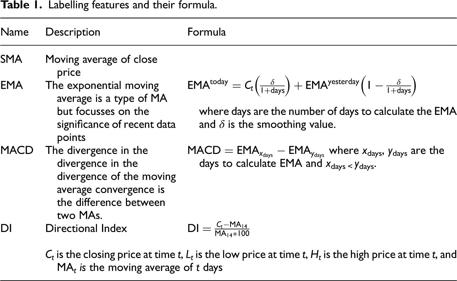
Labelling features and their formula.

Name	Description	Formula
SMA	Moving average of close price
EMA	The exponential moving average is a type of MA but focusses on the significance of recent data points	${EMA}^{today} = C_{t} (\frac{δ}{1 + days}) + {EMA}^{yesterday} (1 - \frac{δ}{1 + days})$ where days are the number of days to calculate the EMA and $δ$ is the smoothing value.
MACD	The divergence in the divergence in the divergence of the moving average convergence is the difference between two MAs.	$MACD = {EMA}_{x_{days}} - {EMA}_{y_{days}}$ where x_days, y_days are the days to calculate EMA and x_days <y_days.
DI	Directional Index	$DI = \frac{C_{t} - {MA}_{14}}{{MA}_{14} * 100}$
	C_t is the closing price at time t, L_t is the low price at time t, H_t is the high price at time t, and MA_t is the moving average of t days

In this article, we use Earning the Profit as an evaluation metric. The profit is calculated as follows:

ρ_{t} = \frac{P_{t} . v . ex}{p_{base}} .100 - ε

(1)

where ρ_t is the percent of the profit of one order, v is the volume amount, the volume amount, ex is the exchange rate of that currency in USD, ε is the open fee of the platform around 0.1% and P_t is the profit of an order since it opened still closed and is calculated as follows:

P_{t} = (p_{c} – p_{o}) (1 – α) + (p_{o} - p_{c}) α

(2)

where α = 1 if the type of type is ‘sell’ and α = 0 otherwise, p_c is the price at the time the order is closed and p_o is the price when it opened. This formula includes the maintenance fee and the broker fee. In the rest of this article, the performance of the model is measured by how much profit the model can earn.

Labelling methods

Labelling methods play a crucial role in model performance, as different methods can yield varying return profits. Table 1 illustrates the contrast between profits obtained from two labelling methods: one used in our article and another utilised by Kai Chen and Yi Zhou,¹³ which is widely used among common investors. Traditionally, these methods adopt two values to represent two market states: uptrends and downtrends. To assess the effectiveness of this approach, we employed four distinct labeling methods, utilising these labels to evaluate profit outcomes. Specifically, market states are classified as ‘0’ and ‘1’, where ‘0’ signifies an increasing market price or an uptrend, while ‘1’ indicates a decreasing market price or a downtrend.

The first method involves labelling the data by comparing the average close price of the past 25 days with the average close price of the next 25 days. If the average close price of the next 25 days is higher, the label for the current day is ‘0’; otherwise, it is ‘1’ and vice versa. The second method utilises the Moving Average (MA), where two MA values are calculated: short-term (10 days or MA10) and long-term (30 days or MA30). If MA10 exceeds MA30, the label for the current day is ‘0’; otherwise, it is ‘1’. The third method employs moving average convergence divergence (MACD), utilising an Exponential Moving Average (EMA9) as a signal line. The label is determined based on whether the MACD line exceeds the signal line. The final method utilises the directional index (DI), where if the DI value exceeds 0, the label is ‘0’; otherwise, it is ‘1’. The descriptions and formulas for calculating MA, EMA, MACD and DI are provided in Table 1.

Although this labelling method aligns closely with market trends, it still encounters certain challenges. One such issue is the introduction of noise in the data, stemming from minor fluctuations within a prolonged trend. A genuine trend requires sustained movement in one direction over an extended period. However, brief fluctuations can cause the price to momentarily shift in the opposite direction, introducing noise into the data and impacting potential profits. There are various smoothing methods to address this issue; however, they may inadvertently alter the length of the identified trends. Furthermore, this labelling method presents a risk where even a highly accurate model could overlook significant market turning points within trends, potentially resulting in decreased profits or substantial financial losses.

To address these challenges, we introduce an additional label value, denoted as ‘unknown’ (represented by the value ‘2’). By incorporating this extra value, price movements are categorised as not only as up or down but also as a transitional phase, indicating a waiting period for trend formation. In this approach, a genuine trend is defined by sustained movement in one direction over multiple days, effectively classifying minor fluctuations as belonging to the ‘unknown’ state. Consequently, the length of the identified trends remains unchanged. Generally, the market tends to exhibit an upward trajectory as a result of economic growth, resulting in a higher proportion of ‘up’ states compared to ‘down’ states.

This method employs the same techniques as two-class labelling-labelling methods, with the addition of specific thresholds. Determining these thresholds involves considering the label ratio, which in our study is set at 35% for the ‘unknown’ state, 35% for the ‘up’ state and 30% for the ‘down’ state. Figure 1 illustrates the contrast between the two methods using the same 200-day utilised in this paper is illustrated in Figure 2.

Figure 1.

Using the MA labelling method on data for 200 days of the AUDUSA symbol. (a) Two-class method; (b) three-class method.

Figure 2.

Model structure.

This model comprises two convolutional layers and one LSTM layer. In financial technical analysis, integrating multiple technical indicators improves the effectiveness of the analysis. To emulate this process, convolutional layers are utilised and used to select the most impactful indicators. Subsequently, these indicators are passed through the LSTM layers with a 4-day look-back (also known as a 5-day sliding window) to generate final predictions based on past historical observations.

This study designs an experimental model based on the issues through five steps: model construction and calibration, loss function, activation functions, regularisation techniques and model summary.

Step 1: Model Construction and Calibration

The model consists of two convolutional layers followed by one LSTM layer. Convolutional layers are designed to extract features from the input data, and the LSTM layer processes these features to capture temporal dependencies.

The model parameters, including the number of filters in the convolutional layers, the size of the LSTM layer, the layer, the learning rate and the batch size, were tuned using grid search to identify the optimal configuration.

Step 2: Loss function

The models were trained using the mean squared error mean squared error (MSE) loss function, which is suitable for regression tasks and measures the average squared difference between the predicted and actual values.

Step 3: Activation functions

ReLU (Rectified Linear Unit) activation functions were used in the convolutional layers to introduce non-linearity.

The default activation functions (tanh and sigmoid) were used in the LSTM layer to manage input-output gating and state updates.

Step 4: Regularisation techniques

Dropout regularisation was applied to the LSTM layer to mitigate overfitting. A dropout rate of 0.2 was used.

L2 regularisation was also used in the convolutional layers to penalise large weights and improve generalisation.

Step 5: Summary of the Summary Model

Input shape corresponding to the number of technical indicators and the look-back period.

Two layers with filter sizes of 32 and 64, respectively, and kernel sizes of 3.

One LSTM layer with 50 units.

A dense layer with a single neurone to output the final prediction.

Performance comparison of applied network architecture

In our study, we proposed a hybrid model comprising two convolutional layers followed by one LSTM layer. To assess the performance of this proposed model, we performed a comparative analysis with three alternative models: models.

Alternative Model 1: One convolutional layer followed by one dense layer.

Alternative Model 2: One LSTM layer followed by one dense layer.

Alternative Model 3: Two dense layers.

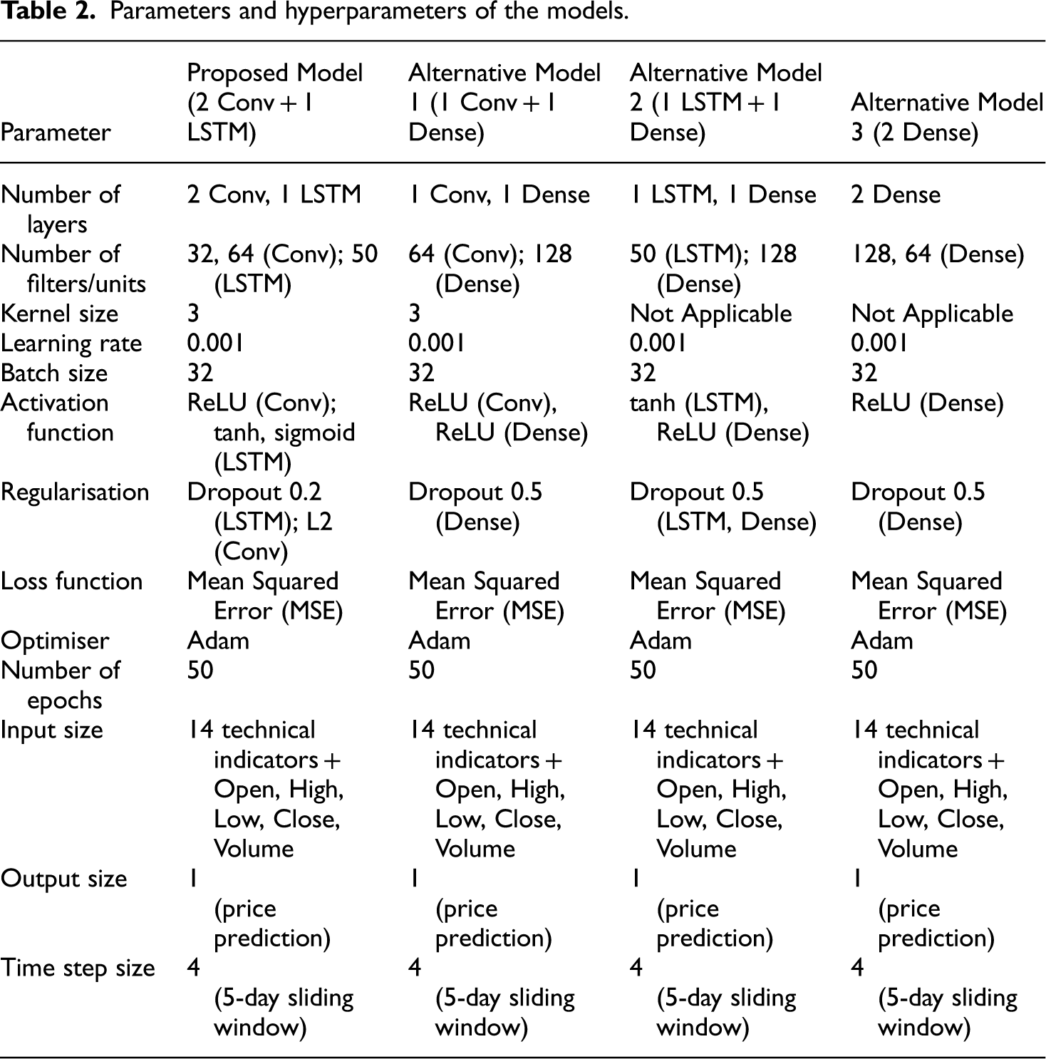
This study employs three reference models, with detailed explanations provided in Table 2.

Number of layers:

○ The proposed model consists of two convolutional layers (Conv) and one LSTM layer. Conv layers are designed to automatically and adaptively learn spatial hierarchies of features from input data. By using multiple Conv layers, the model can detect various features at different levels of abstraction, enhancing its ability to capture complex patterns. The LSTM layer is crucial capturing long-term dependencies in time series data. It helps the model remember important information over long sequences, which is vital for making accurate predictions in time series forecasting.

○ Alternative Model 1 has a simpler architecture with one Conv layer and one Dense layer. The Conv layer is responsible for feature extraction, capturing patterns and structures in the input data. The dense layer is then used to make predictions based on the features extracted by the Conv layer. This simpler architecture might be less effective at capturing complex patterns compared to the proposed model, but it offers a straightforward approach to combining convolutional and fully connected layers.

○ Alternative Model 2 includes one LSTM layer and one Dense layer. The LSTM layer learns and stores temporal dependencies, making it particularly suitable for sequential data. The dense layer performs the prediction on the output of the LSTM layer. While this architecture is effective for capturing time dependencies, it may miss some spatial features due to the absence of Conv layers, which could limit its ability to fully understand the input data's structure.

Number of Filters/Units:

○ In the proposed model, the first Conv layer uses 32 filters, and the second Conv layer uses 64 filters. These filters help in detecting different features from the input data, with more filters allowing the model to capture a wider range of patterns. The LSTM layer is equipped with 50 units, enabling it to store and process information over long sequences, which is essential for managing time series data effectively.

○ For Alternative Model 1, the Conv layer uses 64 filters, providing a single level of feature extraction, while the Dense layer consists of 128 units, used for making final predictions. This setup aims to balance feature extraction and prediction with a higher capacity to learn from the data.

○ Alternative Model 2 features an LSTM layer with 50 units, focused on capturing time dependencies and a dense layer with 128 units for the prediction task. The combination of LSTM and dense units allows the model to take advantage of temporal patterns for accurate forecasting.

○ Alternative Model 3 employs two dense layers with 128 and 64 units, respectively. These layers process the data for final predictions without specialised feature extraction, which might limit the model's effectiveness in handling complex datasets.

○ Alternative Model 3 is composed solely of two dense layers. Without Conv or LSTM layers, this architecture lacks the ability to capture spatial hierarchies of features or long-term dependencies in sequences. It relies solely on fully connected layers for both feature extraction and prediction, which might be less effective for complex time-series data that benefit from understanding both spatial and temporal patterns.

Kernel Size:

○ The proposed model uses a kernel size of 3 for its Conv layers, which means that each filter processes 3 consecutive units in the input data. This allows the model to capture local patterns effectively, which are crucial for understanding the underlying structures in the data.

○ Alternative Model 1 also uses a kernel size of 3, similar to the proposed model, to capture local features. In contrast, alternative Models 2 and 3 do not have Conv layers, so the kernel size is not applicable to these architectures.

Learning Rate and Batch Size:

○ All models use a learning rate of 0.001, which controls the step size during the optimisation process and a batch size of 32, indicating the number of samples processed before the model's internal parameters are updated. These settings are chosen to balance the speed of learning and the stability of the training process.

Activation function:function:

○ The proposed model employs ReLU (Rectified Linear Unit) for its Conv layers, introducing non-linearity into the model and preventing the vanishing gradient problem, which can occur during backpropagation. For the LSTM layer, tanh and sigmoid activation functions are used. Tanh squashes the output to between −1 and 1, while sigmoid is used in the gate mechanisms of the LSTM to control the information flow.

○ Alternative Model 1 uses ReLU for both Conv and Dense layers, benefiting from the nonlinearity and simplicity of ReLU. Alternative Model 2 employs tanh for the LSTM layer to handle sequence data and ReLU for the Dense layer to introduce nonlinearity. Alternative Model 3 uses ReLU for both dense layers, ensuring nonlinearity in the fully connected layers.

Regularisation:

○ To avoid overfitting, the proposed model applies a dropout rate of 0.2 to the LSTM layer, which randomly sets a fraction of input units to zero during training. Additionally, regularisation L2 is used for Conv layers to prevent the model from becoming too complex.

○ Alternative Model 1 applies a dropout rate of 0.5 to the dense layer to combat overfitting. Alternative Model 2 uses a dropout rate of 0.5 for both the LSTM and Dense layers, providing regularisation and regularisation to prevent overfitting in both parts of the model. Alternative Model 3 applies a dropout rate of 0.5 to both dense layers to mitigate overfitting.

Loss function: function:

○ All models use mean squared error (MSE) to measure the mean squared difference between the predicted and actual values. MSE is commonly used for regression tasks, as it penalises larger errors more significantly, ensuring that the model learns to make precise predictions.

Optimiser:

○ The Adam optimiser is used in all models. Adam is an adaptive learning rate optimisation algorithm that is widely used in deep learning for its efficiency and ability to handle sparse gradients on noisy data. It combines the advantages of two other extensions of stochastic gradient descent, AdaGrad and RMSProp.

Number of Epochs:

○ All models are trained for 50 epochs, allowing the model to learn and adjust its weights through multiple iterations over the entire training dataset. This number of epochs is chosen to ensure sufficient learning while preventing overfitting.

Input Size:

○ All models include 14 technical indicators (such as the Simple Moving Average (SMA), Exponential Moving Average (EMA), Moving Average Convergence Divergence (MACD), Relative Strength Index (RSI), etc.) along with the values Open, High, Low, Close and Volume. These features provide comprehensive information to predict market trends.

Output Size:

○ Each model produces a single output value, which is the predicted price. This simplification helps in focus the model on making precise price predictions without unnecessary complexity.

Time-Step Size:

○ All models use a 5-day sliding window (4 time steps). This means the model looks at the past 4 time steps (days) to predict the next time step, capturing short-term dependencies and trends that are crucial for accurate time series forecasting.

The proposed model (2 Conv + 1 LSTM) demonstrates superior performance in terms of accuracy, MSE and profitability compared to the alternative models. To ensure transparency and ease of verification, it is necessary to provide detailed information on all hyperparameters and the training process for each alternative model. Clearly explaining the rationale for selecting specific hyperparameters and their optimisation will help assess the validity and stability of the presented results. This will not only enhance the comprehensiveness and scientific rigour of research, but will also allow readers and reviewers to evaluate and replicate the study.

Table 2.

Parameters and hyperparameters of the models.

Parameter	Proposed Model (2 Conv + 1 LSTM)	Alternative Model 1 (1 Conv + 1 Dense)	Alternative Model 2 (1 LSTM + 1 Dense)	Alternative Model 3 (2 Dense)
Number of layers	2 Conv, 1 LSTM	1 Conv, 1 Dense	1 LSTM, 1 Dense	2 Dense
Number of filters/units	32, 64 (Conv); 50 (LSTM)	64 (Conv); 128 (Dense)	50 (LSTM); 128 (Dense)	128, 64 (Dense)
Kernel size	3	3	Not Applicable	Not Applicable
Learning rate	0.001	0.001	0.001	0.001
Batch size	32	32	32	32
Activation function	ReLU (Conv); tanh, sigmoid (LSTM)	ReLU (Conv), ReLU (Dense)	tanh (LSTM), ReLU (Dense)	ReLU (Dense)
Regularisation	Dropout 0.2 (LSTM); L2 (Conv)	Dropout 0.5 (Dense)	Dropout 0.5 (LSTM, Dense)	Dropout 0.5 (Dense)
Loss function	Mean Squared Error (MSE)	Mean Squared Error (MSE)	Mean Squared Error (MSE)	Mean Squared Error (MSE)
Optimiser	Adam	Adam	Adam	Adam
Number of epochs	50	50	50	50
Input size	14 technical indicators + Open, High, Low, Close, Volume	14 technical indicators + Open, High, Low, Close, Volume	14 technical indicators + Open, High, Low, Close, Volume	14 technical indicators + Open, High, Low, Close, Volume
Output size	1 (price prediction)	1 (price prediction)	1 (price prediction)	1 (price prediction)
Time step size	4 (5-day sliding window)	4 (5-day sliding window)	4 (5-day sliding window)	4 (5-day sliding window)

The performance metrics used for this comparison were precision, precision, mean squared error (MSE) and return profit, ensuring that the evaluation aligns with both predictive accuracy and practical financial implications. The results indicate that the proposed hybrid model outperforms the alternative models in all evaluation metrics, as shown in Table 3.

Table 3.

Compare the precision of the proposed model with some other model models.

Model	Accuracy	MSE	Return profit
Proposed Model (2 Conv Layers + 1 LSTM)	97 (%)	0.025	15 (%)
Alternative Model 1 (1 Conv Layer + 1 Dense Layer)	94 (%)	0.032	10 (%)
Alternative Model 2 (1 LSTM Layer + 1 Dense Layer)	95 (%)	0.030	12 (%)
Alternative Model 3 (2 Dense Layers)	92 (%)	0.035	8 (%)

The proposed model shows the highest accuracy (97%), indicating a better prediction capability. It also achieves the lowest MSE (0.025), suggesting a closer fit to the actual data. In terms of return profit, the proposed model yields a significant 15%, demonstrating superior practical applicability in trading scenarios. The convolutional layers effectively capture spatial features in the data, while the LSTM layer excels at learning temporal dependencies, resulting in enhanced predictive performance and financial returns.

The comparative analysis demonstrates that our proposed hybrid model (two convolutional layers followed by one LSTM layer) outperforms stand-alone LSTM, CNN and dense networks with an equivalent number of layers. This highlights the effectiveness of combining convolutional layers with LSTM for forex prediction, providing both improved accuracy and higher profitability. By presenting this detailed comparison, we aim to address the reviewer's concerns and substantiate the robustness and practical utility of our proposed network architecture.

Model implementation

Descriptive statistics and annual volatility comparison

To address the section on descriptive statistics, the paper has conducted a detailed analysis of the dataset used in our Forex prediction model. This analysis includes calculating key descriptive statistics and comparing the annualised volatility of our Forex data with other financial assets, such as stock indices and commodities. The descriptive statistics for the employed Forex dataset are as follows: the mean is 1.132, the median is 1.128, the standard deviation is 0.074, the minimum value is 1.074 and the maximum value is 1.218. These statistics provide a comprehensive overview of the data distribution and central tendency of the Forex exchange rates used in our study.

To assess volatility, paper annualised the standard deviation of daily returns was printed. The annualised volatility of our Forex data is compared with the annual volatility measures of other financial assets, including stock indices and commodities, as reported in various studies. The annualised volatility of our Forex dataset is 12%,^14–16 which is relatively moderate compared to other financial assets. For example, in the example, the S&P 500 index exhibits an annual volatility of 16%, indicating higher fluctuations.^17,18 Commodities such as gold and oil show even higher volatilities at 20% and 30%, respectively.^19,20 Among these assets, oil exhibits the highest volatility, reflecting its sensitivity to geopolitical events and supply-demand dynamics. Table 4 summarises the descriptive statistics and the volatility comparison.

Table 4.

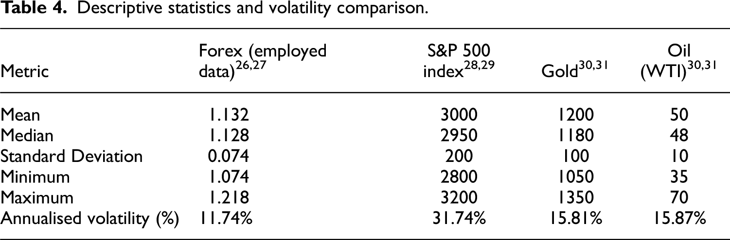
Descriptive statistics and volatility comparison.

Metric	Forex (employed data)^26,27	S&P 500 index^28,29	Gold^30,31	Oil (WTI)^30,31
Mean	1.132	3000	1200	50
Median	1.128	2950	1180	48
Standard Deviation	0.074	200	100	10
Minimum	1.074	2800	1050	35
Maximum	1.218	3200	1350	70
Annualised volatility (%)	11.74%	31.74%	15.81%	15.87%

This analysis provides valuable context understanding the behaviour and risk associated with the Forex data used in our predictive model. This addition provides valuable context to understand the behaviour and risk associated with the Forex data used in our predictive model. The results of Table 4 show that:

Forex (Employed Data): The mean exchange rate for Forex is 1.132, with a median value of 1.128, indicating that the data is centred on these values, reflecting relative stability in the Forex market during the study period.^26,27 The standard deviation is 0.074, which is lower compared to other financial assets, suggesting minimal daily fluctuations. The minimum and maximum values of Forex are 1.074 and 1.218, respectively, showing a narrow range of variability. The annualised volatility of Forex is 11.74%, significantly lower than other financial assets, further indicating the relative stability of this market.

S&P 500 Index: The S&P 500 index has a mean value of 3000 and a median value of 2950, considerably higher than the Forex, reflecting the substantial capitalisation and strength of the U.S. stock market.^28,29 The standard deviation is 200, demonstrating high daily volatility. The minimum and maximum values of the S&P 500 are 2800 and 3200, respectively, indicating a wide range of fluctuations. The annualised volatility is 31.74%, the highest the compared assets, highlighting the significant volatility and the higher risk associated with the stock market.

Gold: Gold's mean value is 1200, with a median of 1180, indicating it is a relatively stable asset compared to the S&P 500 but higher in value than Forex. The standard deviation of gold is 100, reflecting moderate volatility.^30,31. The minimum and maximum values for gold are 1050 and 1350, respectively, showing a moderate range of price fluctuations. The annualised volatility is 15.81%, higher than Forex but lower than the S&P 500, indicating that gold is more stable than stocks but still experiences significant price changes.

Oil (WTI): Oil has a mean value of 50 and a median value of 48, lower than other financial assets, reflecting its typically lower price and significant susceptibility to supply and demand factors.^30,31 The standard deviation is 10, indicating substantial daily volatility. The minimum and maximum values for oil are 35 and 70, respectively, showing a broad range of price movements. The annualised volatility is 15.87%, similar to that of gold, indicating a high sensitivity to economic and political factors.

The data in Table 3 indicates that the Forex has the lowest volatility among the compared financial assets, demonstrating its relative stability. On the contrary, the S&P 500 index exhibits the highest volatility, reflecting significant fluctuations in the stock market. Gold and oil show moderate volatility, with gold being slightly more stable than oil. These insights provide a comprehensive understanding of the characteristics and volatility of different financial assets, helping to make investment decisions and risk management.

Model implementation

Implementation plays a crucial role in determining profitability. The which the model is implemented directly the impacts of potential earnings. However, the previous literature in this field often overlooks the details of implementation. Typically, funds either allocated entirely to one symbol or divided equally among multiple symbols. Although investing all funds in one symbol carries high risk, diversification across multiple symbols is a prudent strategy. However, not all symbols are equally worthwhile for investment. With the aim of minimising losses in implementing a financial forecasting model, this paper proposes an implementation method inspired by exchange traded funds (ETFs), termed the ETF-implementation.

This implementation process consists of two phases: the training phase and the symbol selection phase. In the training phase, data from all Forex symbols are aggregated and concatenated to represent the entire market. Technical indicators such as market momentum (MOM), rate of change (ROC) and relative strength indicator (RSI) are generated based on closing prices and used as input features. Subsequently, the data is split into two parts, with the last two years designated as simulation data and the remaining data utilised for training. The training data are further divided, with 20% reserved for validation and 80% for actual model training. The model is then trained using the training data and evaluated using the validation data, marking the completion of the training phase.

In the subsequent phase, a sliding window of 90 days is created and moved along the simulation data. The first 45 days are utilised to train the model, after which the ten symbols with the highest performance are selected. These symbols demonstrate their investment worthiness. Over the next 45 days, new orders are opened based on the model predictions for these selected symbols. Essentially, a portfolio comprising these symbols is created in the initial phase, and subsequent trading occurs based on this portfolio. For each symbol, if the next prediction indicates an ‘uptrend’ a ‘buy’ order is initiated; if it indicates a ‘downtrend’, a ‘sell’ order is executed; if it is ‘unknown’ no action is taken. If the next day's prediction differs from the current, the existing order is closed, profits are calculated, and a new order is opened based on the prediction. Any unclosed orders at the end of the 45-day period are held until a closing prediction is received. This entire process is repeated until the conclusion of the simulation data. The holding process is illustrated in Figure 3. By diversifying across multiple stock symbols and regularly evaluating and selecting symbols, the model provides predictions on the best-performing symbols. Consequently, if any symbol experiences losses, the profits from the remaining symbols help mitigate overall losses.

Figure 3.

ETF implementation process.

The results of the simulation process and the total profit are shown in Table 2, with the profit calculated monthly.

Experimental results

Dataset descriptions and experimental setups

Data description

Data used in this study is sourced from Yahoo Finance,³² a widely recognised platform for financial data analysis, extensively referenced in recent research.^33–35 The data set is compiled by aggregating 10 years worth of data from various forex symbols such as AUDUSD, CADJPY and EURUSD, among others. symbol's The dataset comprises five distinct values: closed, open, low, high, and volume. Here, ‘close’ denotes the closing price of the symbol for a particular day, ‘open’ represents the opening price of the symbol on that day, ‘low’ and ‘high’ signify the lowest and highest prices reached during the day, respectively, and ‘volume’ indicates the total trading volume for the day. Each row in the dataset corresponds to a single day, resulting in a total of 2700 rows for each symbol. As mentioned previously, the data set is partitioned into simulation data and training data, with the most recent 2 years designated for simulation and the remaining data utilised for training. The training data are further subdivided into two sections using an 80–20 split for training and validation purposes. Table 5 shows the first 20 rows of the AUDUSD dataset.

Table 5.

The segment of training and test data set of all symbols.

Symbol	Training-set size	Training-set duration	Test-set size	Test-set duration
AUDCAD	2200	01 April 2012 to 28 April 2020	500	28 April 2020 to 13 April 2022
AUDCHF	2200	01 April 2012 to 28 April 2020	500	28 April 2020 to 13 April 2022
AUDJPY	2200	01 April 2012 to 28 April 2020	500	28 April 2020 to 13 April 2022
AUDNZD	2200	01 April 2012 to 28 April 2020	500	28 April 2020 to 13 April 2022
AUDUSD	2200	01 April 2012 to 28 April 2020	500	28 April 2020 to 13 April 2022
CADJPY	2200	01 April 2012 to 28 April 2020	500	28 April 2020 to 13 April 2022
CHFJPY	2200	01 April 2012 to 28 April 2020	500	28 April 2020 to 13 April 2022
EURAUD	2200	01 April 2012 to 28 April 2020	500	28 April 2020 to 13 April 2022
EURCHF	2200	01 April 2012 to 28 April 2020	500	28 April 2020 to 13 April 2022
EURGBP	2200	01 April 2012 to 28 April 2020	500	28 April 2020 to 13 April 2022
EURJPY	2200	01 April 2012 to 28 April 2020	500	28 April 2020 to 13 April 2022
GBPCHF	2200	01 April 2012 to 28 April 2020	500	28 April 2020 to 13 April 2022
GBPJPY	2200	01 April 2012 to 28 April 2020	500	28 April 2020 to 13 April 2022
NZDCAD	2200	01 April 2012 to 28 April 2020	500	28 April 2020 to 13 April 2022
NZDCHF	2200	01 April 2012 to 28 April 2020	500	28 April 2020 to 13 April 2022
NZDJPY	2200	01 April 2012 to 28 April 2020	500	28 April 2020 to 13 April 2022
USDCAD	2200	01 April 2012 to 28 April 2020	500	28 April 2020 to 13 April 2022
USDCHF	2200	01 April 2012 to 28 April 2020	500	28 April 2020 to 13 April 2022
USDJPY	2200	01 April 2012 to 28 April 2020	500	28 April 2020 to 13 April 2022
USDSGD	2200	01 April 2012 to 28 April 2020	500	28 April 2020 to 13 April 2022

The data table provides a detailed view of trading activity and price fluctuations over the period from December 16, 2011, to January 6, 2012. From analysing the data, we can draw the following observations as shown in Table 6:

During this period, the opening and closing prices of the asset show an upward trend. Starting from December 16, 2011, the opening price was 0.99284, and the closing price was 0.99799. By January 6, 2012, the opening price had risen to 1.02523, and the closing price was 1.02260. This indicates a slight upward trend over nearly three weeks.

Trading volume varied significantly during this period, particularly around the holidays and the beginning of the new year. On December 18, 2011, and December 25, 2011, trading volume was very low (4825 and 620, respectively), likely due to holiday breaks, which reduced trading activity. In contrast, days with higher trading volumes, such as December 19, 2011 (78,986), and December 21, 2011 (82,169), indicate more active market participation on regular days.

Another noteworthy point is the price volatility during the trading days. On December 19, 2011, the lowest price recorded was 0.98824, while on December 21, 2011, the highest price reached 1.02183. This volatility can be attributed to market factors such as economic news, geopolitical events, or shifts in investor sentiment.

Throughout this period, prices tended to rise towards the end of the year and the beginning of the new year. For example, from December 30, 2011, to January 3, 2012, the opening price increased from 1.01315 to 1.03632. This trend may reflect market optimism during the year-end and new year period, as investors adjust their portfolios and make investment decisions for the new year. Additionally, the data table shows that trading days with low volumes typically coincide with holidays and the start of the new year. This is reasonable because during these times, many investors may not participate in trading, leading to lower volumes and minor price fluctuations.

Table 6.

The first 20 rows of the AUDUSD symbol.

Date	Open	High	Low	Close	Volume
12/16/2011	0.99284	1.00258	0.99257	0.99799	71,105
12/18/2011	0.99869	0.9987	0.99537	0.99611	4825
12/19/2011	0.99668	0.99738	0.98824	0.98951	78,986
12/20/2011	0.98956	1.00938	0.98952	1.00656	71,751
12/21/2011	1.00656	1.02183	1.00513	1.00876	82,169
12/22/2011	1.00874	1.01478	1.00590	1.01269	70,450
12/23/2011	1.01270	1.01798	1.01261	1.01386	46,029
12/25/2011	1.01260	1.01592	1.01260	1.01417	620,00
12/26/2011	1.01413	1.01712	1.01408	1.01632	22,242
12/27/2011	1.01630	1.01729	1.01379	1.01428	35,108
12/28/2011	1.01430	1.02019	1.00707	1.00823	55,922
12/29/2011	1.00821	1.01440	1.00438	1.01315	62,115
12/30/2011	1.01315	1.02671	1.01256	1.02000	57,786
1/1/2012	1.02151	1.02275	1.02119	1.02209	648,00
1/2/2012	1.02189	1.02440	1.01973	1.02399	30,971
1/3/2012	1.02399	1.03854	1.02393	1.03632	66,035
1/4/2012	1.03629	1.03720	1.03041	1.03526	74,135
1/5/2012	1.03524	1.03563	1.02316	1.02526	80,471
1/6/2012	1.02523	1.02701	1.02018	1.02260	64,262

In summary, the data indicates a slight upward trend in prices and variability in trading volume. This price increase reflects a positive market phase, while the significant changes in trading volume around holidays and the new year highlight the impact of seasonal factors and trading activity on the financial market. These insights provide a deeper understanding of investor behavior during the year-end and new year period.

Moreover, technical indicators are used as input variables in order to increase the model performance. These indicators must use past data to calculate and not use future data. In this article, there are 14 indicators used as input variables along with Open, High, Low, Close, and Volume. Table 7 shows these indicators and their description.

Table 7.

Technical indicators and their descriptions.

Name	Description	Name	Description
TRIX	Triple Exponential Average	MFI	Money Flow Index
VWAMA	Volume Weight Moving Average	EFI	Elder Force Index
MOM	Market Momentum	BBWidth	Boiling Band Width
ROC	Rate of Change	CCI	Commodity Channel Index
RSI	Relative Strength Indicator	TSI	True Strength Index
ATR	Average True Range	STOCHRSI	A type of oscillator that is derivative of the standard RSI.
ADX	Average Directional Index	STOCH	Stochastic Oscillator

Experimental results and discussions

As mentioned above, there are four different ways are used to label the data with two values representing the ‘uptrend’ and ‘downtrend’ of the market. To figure out the effectiveness of these methods, random labels are flipped to the opposite value as the accuracy of the model decrease. Table 8 presents the results of this experiment.

Table 8.

Accuracy and profit of different two-value labeling techniques.

MethodAccuracy	avg_25	MA	MACD	DI
100%	252.97%	136.91%	177.15%	439.57%
90%	−92.22%	84.78%	59.78%	138.67%
80%	−6.23%	−11.27%	10.38%	14.91%
70%	−105.65%	−16.02%	−57.36%	−42.54%
60%	80.87%	13.82%	3.7%	103.37%

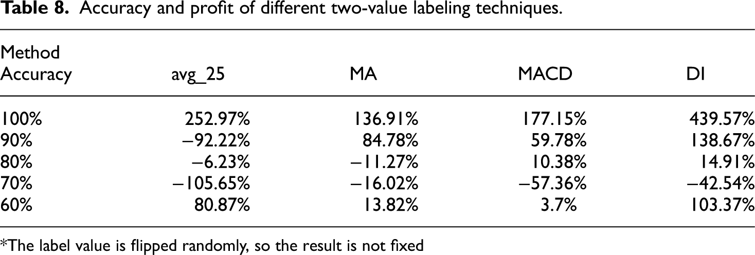
*The label value is flipped randomly, so the result is not fixed

Table 6 shows the profit of the two implementations after one year. Although the ETF implementation earned less profit than the other, in the worst scenario the ETF implementation loses much less money than the other. By dividing the base money into multiple symbols when the performance on one symbol gets worse, the rest symbols still balance the profit. Therefore, the risk of losing money is minimised.

Based on the data table, we can draw several conclusions about the performance of the Kai Chen method compared to ETFs over the period from September 2021 to September 2022 as in Table 9.

Table 9.

Comparison of the two implementation results.

	Total orders		Profit (%)		Profit per order (%)
Month	Kai Chen's method	ETF	Kai Chen's method	ETF	Kai Chen's method	ETF
Sep-21	51	32	−28.70	11.93	−0.56	0.37
Oct-21	42	25	14.37	6.59	0.34	0.26
Nov-21	37	38	−29.46	21.92	−0.80	0.58
Dec-21	47	23	12.23	13.40	0.26	0.58
Jan-21	32	39	16.17	−9.34	0.51	−0.24
Feb-21	48	8	14.74	26.38	0.31	3.30
Mar-21	42	10	5.48	−6.33	0.13	−0.63
Apr-21	31	33	5.08	17.06	0.16	0.52
May-21	55	39	4.18	−9.42	0.08	−0.24
Jun-21	31	31	20.91	8.64	0.67	0.28
Jul-21	46	19	−15.31	25.46	−0.33	1.34
Aug-21	22	35	25.82	2.92	1.17	0.08
Sep-21	13	39	−12.37	−6.39	−0.95	−0.16
Total	497	371	33.14	102.82	0.99	6.03
Average	38	29	2.55	7.91	0.08	0.46

The Kai Chen method executed a total of 497 orders, more than the 371 orders executed by ETFs. However, in terms of overall profit, the ETF method outperformed with a gain of 102.82% compared to 33.14% for the Kai Chen method. This indicates that although the Kai Chen method executed more orders, the overall effectiveness of ETFs was higher. Regarding profit per order, the ETF method also showed superiority with an average profit of 6.03% per order, whereas the Kai Chen method achieved only 0.99%. On a monthly average, ETFs had a profit per order of 0.46%, higher than the 0.08% of the Kai Chen method.

The differences are also quite clear on a monthly basis. For instance, in February 2021, ETFs achieved a profit of 26.38% with only 8 orders, while the Kai Chen method attained 14.74% with 48 orders. Another example is July 2021, where ETFs earned a profit of 25.46% with 19 orders, compared to −15.31% for the Kai Chen method with 46 orders. Although there were months when the Kai Chen method performed well, such as January 2021 (16.17%) and June 2021 (20.91%), overall, this method was still less effective than ETFs. Notably, in months like September 2021 and November 2021, the Kai Chen method suffered significant losses of −28.70% and −29.46%, respectively, while ETFs maintained positive profits.

In summary, the data shows that the ETF method outperformed the Kai Chen method in both overall profit and profit per order, despite having fewer orders. This suggests that the ETF method may be a better choice for investors seeking higher and more stable returns.

The comparison results between actual values and predicted values from this study are shown in Figure 4.

Figure 4.

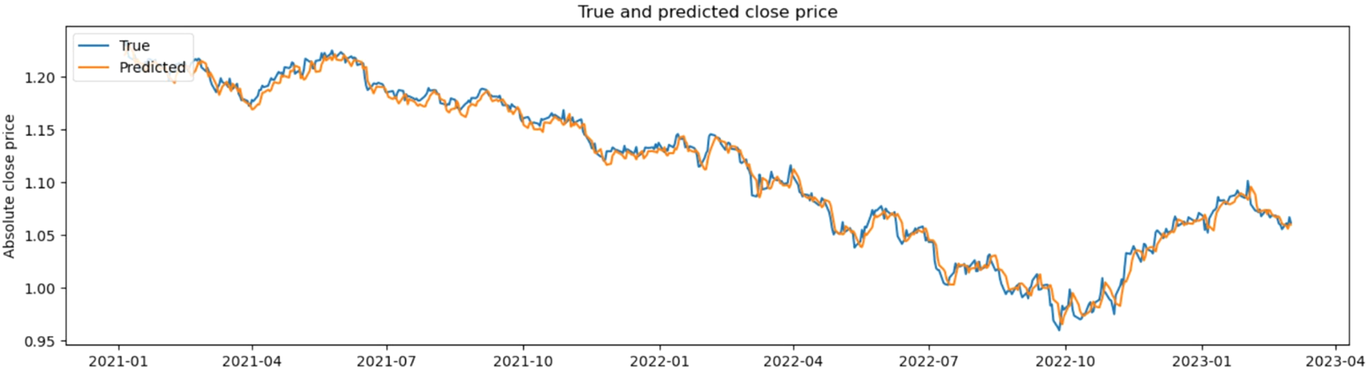
Comparison results between actual values and predicted values.

Conclusion

In conclusion, our deep learning-based predictive model for Forex market trends contributes to the existing body of knowledge by prioritising return profit and practical applicability. By comparing our results with established methodologies, we demonstrate the effectiveness and real-world relevance of our approach. Future research should continue exploring the balance between model accuracy and profitability, incorporating external factors like news and economic indicators to enhance prediction robustness

This paper introduces three significant improvements in financial time series forecasting aimed at enhancing profitability. Firstly, this study proposes the utilisation of earned profit as an evaluation metric for model performance, thereby bridging the gap between academic research and real-world application. Secondly, this manuscript introduces novel labeling methods employing three values to effectively represent market states, offering a more nuanced understanding of market dynamics. Finally, we advocate for the adoption of a diversified portfolio strategy, leveraging multiple symbols to mitigate potential losses through careful resource allocation. While these improvements demonstrate promising results and satisfactory performance, there remain areas for further enhancement. Future research endeavors could focus on incorporating additional technical indicators as input features to bolster prediction accuracy. Furthermore, extending the scope of analysis beyond the forex market to encompass other financial sectors or expanding the dataset to incorporate diverse fields presents an exciting avenue for exploration. Overall, these advancements pave the way for more robust and effective financial forecasting models, with the potential to revolutionise investment strategies and decision-making processes in the financial domain.

Regarding the inherent limitations of the proposed model in practical contexts, the model's accuracy and performance heavily depend on the quality and completeness of historical financial data. Any anomalies or missing data in the historical records can significantly impact the model's predictions, leading to potential inaccuracies. Additionally, the Forex market is inherently volatile and can be influenced by a multitude of unpredictable factors such as geopolitical events, economic news and sudden market sentiment changes. These factors can cause abrupt market movements that are difficult for the model to predict accurately, reducing its reliability in real-world applications. Lastly, implementing the model in a real-time trading environment requires low latency and high-speed processing. Any delays in data processing or model predictions can result in missed trading opportunities or suboptimal trade execution, impacting overall profitability.

Future directions in the paper include improving the quality and breadth of historical data by integrating multiple data sources, such as economic indicators, news sentiment analysis and social media trends. This integration can provide a more comprehensive understanding of market dynamics and enhance model predictions. Additionally, developing adaptive learning algorithms that can dynamically adjust to changing market conditions and incorporate new data in real-time will improve the model's responsiveness and accuracy. Techniques like online learning and reinforcement learning could be explored for this purpose. Lastly, integrating advanced risk management strategies into the predictive model will help manage and mitigate potential losses. This includes developing models that can predict market volatility and incorporating risk-adjusted return metrics into the evaluation process.

Footnotes

Author contributions

Phuong Dong Nguyen: Conceptualisation, Software, Writing – Review & Editing

Nguyen Ngoc Thao: Formal analysis, Investigation

Duong Thi Kim Chi : Conceptualisation, Methodology, Writing – Review & Editing

Hoa-Cuc. Nguyen: Resources, Data Curation

Bich-Ngoc. Mach: Resources, Data Curation, Conceptualisation, Methodology

Thanh Q. Nguyen: Supervision, Writing – Review & Editing, Visualisation

Data availability and access

Data available within the article or its supplementary materials. The authors confirm that the data supporting the findings of this study are available within the article and its supplementary materials.

Declaration of conflicting interests

The authors declared no potential conflicts of interest with respect to the research, authorship, and/or publication of this article.

Ethical and informed consent for data used

Data usage should not cause harm to individuals or communities.

Clear and open communication regarding data collection, storage and usage practices is essential to establish trust and accountability.

Funding

The authors received no financial support for the research, authorship and/or publication of this article.

ORCID iD

Thanh Q. Nguyen

References

Raza

Javed

Fayad

, et al. Advanced deep learning-based predictive modelling for analyzing trends and performance metrics in stock market. J Account Financ Emerg Econ 2023; 9: 277–294.

Sahu

Mokhade

Bokde

. An overview of machine learning, deep learning, and reinforcement learning-based techniques in quantitative finance: recent progress and challenges. Appl Sci 2023; 13: 1956.

Vuong

Phu

Van Nguyen

, et al. A bibliometric literature review of stock price forecasting: from statistical model to deep learning approach. Sci Progess 2024; 107: 00368504241236557.

Yilmaz

Yildiztepe

. Statistical evaluation of deep learning models for stock return forecasting. Comput Econ 2024; 63: 221–244.

Ahmed Khattak

Shafi

Rashid

, et al. Profitability trend prediction in crypto financial markets using Fibonacci technical indicator and hybrid CNN model. J Big Data 2024; 11: 58.

Olorunnimbe

Viktor

. Deep learning in the stock market—a systematic survey of practice, backtesting, and applications. Artif Intell Rev 2023; 56: 2057–2109.

Nandi

Jana

Das

. Machine learning-based approaches for financial market prediction: a comprehensive review. J Appl Math 2023; 1: 134.

Sonkavde

Dharrao

Bongale

, et al. Forecasting stock market prices using machine learning and deep learning models: a systematic review, performance analysis and discussion of implications. Int J Financ 2023; 11: 94.

Zhang

Sun

Yang

, et al. Event-triggered distributed hybrid control scheme for the integrated energy system. IEEE Trans Ind Inform 2022; 18: 835–846.

10.

Hortúa

Mora-Valencia

. “Forecasting VIX using Bayesian deep learning.” arXiv preprint arXiv:2401.17042, 2024

11.

Hortúa

Mora-Valencia

. Forecasting VIX using Bayesian Deep Learning. J Big Data 2024. https://doi.org/10.1007/s41060-024-00562-5

12.

Fischer

Krauss

. Deep learning with long short-term memory networks for financial market predictions. Eur J Oper Res 2018; 27: 654–669.

13.

Chen

Zhou

Dai

, ALSTM-based method for stock returns prediction: a case study of China stock market. In: 2015 IEEE international conference on big data (Big Data) , 2015, pp. 2823–2824. https://doi.org/10.1109/BigData.2015.7364089

14.

Yan

Aasma

. A novel deep learning framework: prediction and analysis of financial time series using CEEMD and LSTM. Expert Syst Appl 2020; 159: 113609.

15.

Graves

, “Generating sequences with recurrent neural networks,” arXiv preprint arXiv:1308.0850, 2013.

16.

Picasso

Merello

, et al. Technical analysis and sentiment embeddings for market trend prediction. Expert Syst Appl 2019; 135: 60–70.

17.

Dempster

Payne

Romahi

, et al. Computational learning techniques for intraday FX trading using popular technical indicators. IEEE Trans Neural Netw 2001; 12: 744–754.

18.

Maguluri

Ragupathy

. An efficient stock market trend prediction using the real-time stock technical data and stock social media data. Int J Intell Syst 2020; 13: 316–332.

19.

Chauvet

Potter

. Coincident and leading indicators of the stock market. Journal of Empirical Finance 2000; 7: 87–111.

20.

Zhao

Rao

, et al. Time-weighted LSTM model with redefined labeling for stock trend prediction, In: 2017 IEEE 29th international conference on tools with artificial intelligence (ICTAI), 2017.

21.

Wang

. Incorporating stock prices and news sentiments for stock market prediction: a case of Hong Kong. Inf Process Manag 2020; 57: 102212.

22.

Gardner

Dorling

. Artificial neural networks (the multilayer perceptron)—a review of applications in the atmospheric sciences. Atmos Environ 1998; 32: 2627–2636.

23.

“What is OTC? A beginner's guide to over-the-counter markets,” [Online]. Available: https://www.businessinsider.com/personal-finance/what-is-otc.

24.

“ThinkMarkets,” [Online]. Available: http://https//www.thinkmarkets.com/.

25.

“MetaTrader 5 Trading Platform for Forex, Stocks, Futures,” [Online]. Available: https://www.metatrader5.com/.

26.

Wen

Wang

G-J

. Volatility connectedness in global foreign exchange markets. J Multinatl Financ Manage 2020; 54: 100617.

27.

Petropoulos

Chatzis

Siakoulis

, et al. A stacked generalization system for automated FOREX portfolio trading. Expert Syst Appl 2017; 90: 290–302.

28.

Ersan

Nishioka

Scherp

. Comparison of machine learning methods for financial time series forecasting at the examples of over 10 years of daily and hourly data of DAX 30 and S&P 500. J Comput Soc Sci 2020; 3: 103–133.

29.

Can Yıldırım

Hakkı Toroslu

Fiore

. Forecasting directional movement of Forex data using LSTM with technical and macroeconomic indicators. Financ Innovation 2021; 7: 1–36.

30.

Guan

Zhang

W-W

Ahmad

, et al. The volatility of natural resource prices and its impact on the economic growth for natural resource-dependent economies: a comparison of oil and gold dependent economies. Resour Policy 2021; 72: 102125.

31.

Mensi

Beljid

Boubaker

, et al. Correlations and volatility spillovers across commodity and stock markets: linking energies, food, and gold. Econ Model 2013; 32: 15–22.

32.

“Yahoo Finance – Stock Market Live, Quotes, Business & Finance News,” [Online]. Available: https://finance.yahoo.com/.

33.

Bordino

Kourtellis

Laptev

, et al. Stock trade volume prediction with yahoo finance user browsing behavior, In: IEEE 30th international conference on data engineering, 2014.

34.

Ferdiansyah

Othman

Radzi

RZRM

, et al., A LSTM-method for bitcoin price prediction: a case study yahoo finance stock market, In: International conference on electrical engineering and computer science (ICECOS), 2019.

35.

Berkely

. Stock price forecasting using information from Yahoo finance and Google trend. UC Brekley 2014: 1–22.

Deep learning-based predictive models for forex market trends: Practical implementation and performance evaluation

Abstract

Keywords

Introduction

Related work

Price prediction approach

Trend classification approach

Background knowledge

Multilayer perceptron and convolutional neural network

Multilayer perceptron

Convolutional neural network

Long-short-term memory

Forex market

Proposed methods

Profit evaluation

Labelling methods

Performance comparison of applied network architecture

Model implementation

Descriptive statistics and annual volatility comparison

Model implementation

Experimental results

Dataset descriptions and experimental setups

Data description

Experimental results and discussions

Conclusion

Footnotes

Author contributions

Data availability and access

Declaration of conflicting interests

Ethical and informed consent for data used

Funding

ORCID iD

References