Sage Journals: Discover world-class research

Abstract

The water availability concerns have been increasing due to significant impacts of land use land cover change, and climate variability. In terms of developing countries, it is one of the biggest challenges to overcome and manage sustainability in the present and future. This study aims to evaluate the change in hydrological components and simulation of sediment yield and water yield on the large-scale basin of Kotri barrage with a change in runoff due to a change in land use land cover. This study has been done on the watershed as well as the sub-watershed level to have an accurate estimation and simulation by finding the response of hydrological components toward its natural and human-induced factors using the Soil and Water Assessment tool with high-resolution geospatial-temporal inputs over the Kotri catchment. The sediment and water yield were quantified using 42 years of simulation (1981–2022) on the sub-basin level, projected to land use land cover 1990, 2000, 2010, and 2022. The increase in deforestation, agriculture, and settlement areas resulted increase in sediment load in the catchment. The sub-basins 14, 11, 12, and 13, with a high elevation and slope and with less vegetation showed higher sediment load and water yield than the sub-basins with gentle slope and with high natural vegetation cover. The sub-basins 10, 4, and 1 showed high water yield availability compared to basins 2, 3, 5, 6, 7, 8, 9. This may be the result of vegetation differences. However, contained less sediment load than basins 14, 11, 12, and 13. The main objective was to quantify the significant changes affecting catchment and sub-catchment areas, to have a better understanding of the management plan regarding land use land cover. The simulated data was further projected to prediction using machine algorithms (autoregressive integrated moving average) model for precipitation prediction, and (seasonal autoregressive integrated moving average with exogenous factors) model to predict the sediment yield and water yield in the catchment to 2060.

Keywords

Soil and Water Assessment tool land use land cover sediment export water yield autoregressive integrated moving average seasonal autoregressive integrated moving average with exogenous factors

Introduction

Land use land cover (LULC) and climate variability are the main factors in terms of the hydrological response of components. These aspects are essential in any region regulating the hydrological response¹ and are influential over available water resources and flow regimes in river basins all over the world.^2–4

The rapid emergence and widespread climate change, resulting from the rise of natural and human-induced factors in the 21st century,⁵ led to influential changes in hydrological components and many watersheds.⁶ However, alteration in land use land cover (LULC) affects the apportionment of water among diverse hydrological pathways,^7,8 which in turn, leads to change in water distribution, entering through the path of vegetation and soil, such as interception, runoff, infiltration, groundwater recharge,^9,10 soil moisture, soil moisture storage, percolation, lateral flow.^11,12 Hence, it affects runoff generation.¹³

The hydrological behavior in a watershed toward different scenarios needs a high level of understanding. Studies stated that the features of watersheds are significantly responsible for hydrological response differences, whether caused by natural or anthropogenic activities. These features include soil properties, geology, topography, climatic conditions, and anthropogenic activities^14,15

The change in LULC plays a major role in influencing the water movement and sediment yield transportation from designated catchment areas¹⁶ The transformation of landscape into other productive systems like agriculture, and urbanization have significant impacts on soil properties concerning nutrient cycling^17,18 which influences the quality and quantity of water yield¹⁹ in a number of spatial and temporal scales.²⁰ Studies manifested the effects of suspended sediment and nutrient concentration as well.²¹ The transformation of natural land use into deforestation, urbanization, and agriculture are the main LULCs that have been investigated that mainly contribute to influence a specified catchment area.²² The most crucial element of the water cycle is surface runoff which causes soil erosion due to the force of water.²³ Prior studies including^24,25 reported that agriculture and urban expansion are mainly responsible for the increase in surface runoff and reduce percolation and evapotranspiration which in turn increase sediment export within the watershed. When a watershed experiences a change in vegetation cover, it also experiences a change in surface water balance.²⁶ Expansion of cropland, urbanization, and shrunk natural vegetation may cause an increase in surface runoff.^18,27 A Study by Nie et al.²⁸ in the San Pedro Watershed affirmed that the transformation of LULC into residential areas decreased the water yield in 1986, 1992, and 1997, while the increase in agriculture increased runoff.²⁹

A comprehensive and associative approach is essentially needed to have a better understanding of cause and effect of climate variability and LULC change leading to stress on various hydrological elements and sediment export within the watershed. It will help to enhance our understanding regarding climate variability and LULC to adopt effective strategies on a watershed scale, particularly sediment export.³⁰

This study focuses on to evaluate the impacts, examined due to LULC in different spans, and climate variability leading to a change in precipitation patterns in the most important Kotri watershed on a large scale, with an area of 26,068 km². According to Brath et al.³¹ watersheds with an area of 1000 km² require four rain gauges, while according to Dodov and Foufoula-Georgiou³² three rain gauges are needed for a watershed covering an area of 4800 Km². As the Kotri watershed has fewer rain gauges, and due to less availability of data compared to its area, it was challenging to have accurate results and data simulation for the model. To overcome the low data availability maximum weather station points were selected within the boundary.

Material and methods

Study area description

The research has been conducted on the catchment of Kotri barrage, also known as the Ghulam Muhammad barrage, located on the Indus River between Jamshoro and Hyderabad in the province of Sindh Pakistan. Watershed's elevation ranges from −9 to 915 m above sea level. As the biggest barrage of Pakistan, the Kotri is a crucial management structure regulating the flow of water and providing water to millions of people for irrigation. The Major soil types are loam, sandy loam, clay loam, and loamy sand. The land use of the watershed is dominated by cultivated agricultural land Figure 1 shows where the study is located.

Data collection

This study uses both sources of data including primary source data (satellite) and secondary source data (observed for rainfall). The data types were acquired from different data sources. These data types included digital elevation model (DEM), soil, LULC, and weather data, which were used to establish and run the model to execute the required results. The DEM , shuttle radar topography essentially required for the delineation of sub-basin and stream network was obtained from the source of United States Geographical Survey (USGS) with a resolution of 30 m × 30 m. Soil and digital soil map of the world database data acquired from the Food and Agricultural Organization (FAO). Multi-temporal series Landsat images were assessed and analyzed to examine temporal changes in land cover classes for four historical periods of LULC datasets. The multi-temporal datasets selected for each decade were acquired from the source of the USGS with a maximum resolution of 30 m, without any cloud cover. These datasets included Landsat5 thematic mapper (L5-TM) 1990, Landsat7 enhanced thematic mapper plus (L7-ETM+), 2000 and 2010, and Landsat8 Operational Land Imager Thermal Infrared Sensor (L8-OLI-TRS) 2022. These datasets were chosen for the same month and season to avoid seasonal variations (Table 1).

Predicting rainfall, sediment yield, and water yield

Precipitation is considered to be the most important climatic variable that has impacts on the spatial and temporal patterns of water availability,³³ may lead to floods, droughts,³⁴ biodiversity loss, and agricultural productivity hence climatic analysts and water resources planners require special consideration to analyze the trends of precipitation results³⁵ The change in precipitation trend due to changes in LULC and climatic variability leads to the destruction of agricultural productivity and economic development³⁶ Variations in precipitation trends not only damage agriculture productivity and economic loss but also disturb the water cycle as well. Even slight changes in these patterns are found to be effective on regional and global levels. To understand this random mechanism of precipitation we use time series analysis to predict the future using past data.³⁷ The “rainfall prediction” can be defined as the process to predict the amount, time, and location of precipitation using conventional and modern methods,³⁸ including groundwater-based measurements, remote sensing techniques, and several machine-based weather models. Time series forecasting is an essential tool in the field of water resources management. A number of models and methods have been used to predict the precipitation. The shortened time variations in trend can be examined using the autoregressive (AR) and merging average (MA) approaches. Box-Jenkins approach known as AR integrated moving average (ARIMA), is the most essential and widely used time series model. ARIMA is used to simulate different hydrological and meteorological variables.³⁹ ARIMA provides a significant advantage in long-term forecasting. While the sediment yield and water yield forecasting studies are rare to have an idea about the predictive models regarding this variable, seasonal AR integrated moving average with exogenous factors (SARIMAX) is the best selection for forecasting these two variables because of its application of a seasonal ARIMA with exogenous factors Figure 2 shows the Box-Jenkins (ARIMA) model set-ups.

Machine learning and predictive models

Machine learning is an artificial approach based on algorithms and statistics. It enables a non-programmed machine to generate results using given input data. Deep learning is a type of machine learning based on neural network, essential to understand complexity of the data in its patterns and relation. Machine learning as well as deep learning are capable of rainfall forecasting in several ways. Machine algorithms are used to analyze changing patterns and links of historical data that provide more precise forecast results. Both machine learning and deep learning are essential tools in rainfall forecasting, because they have capability to process large amount of data. The machine learning based models provide accurate results as different source data is used to set the model like satellite imaging, radar-based data, and data observed from ground. The machine learning model algorithms allow more specific and localized forecast because these are trained to make predictions at a very granular geographical and spatial scale. Hence algorithms are valuable for a variety of applications, such as water resources management in agriculture and disaster management. However, we face some of the problems regarding management of the data. The basic and primary requirement to test and train the model is the availability of a large quantity data, which is the main problem in rainfall forecasting. This is a difficult task in the region that has less availability of data, especially in developing countries. Despite these problems, machine learning and deep learning prove to be potential approaches to enhance the accuracy and reliability of rainfall forecasting. Several models use several mathematical equations and algorithms produce results based on atmospheric conditions and make weather predictions.³⁸ Weather forecasting and rainfall predictions are very common and important practices nowadays to have a pre-information to control the conditions regarding the situation. For this purpose number of devices are used and trained for rainfall predictions on the basis of weather parameters (temperature, humidity, and wind pressure). Machine algorithms are preferably used because of accurate results with rainfall data analyze in past and forecasting for future, as traditional methods are inefficient methods in most of the cases. However, several techniques are considered depending on the requirement of the study. It is essential to choose a suitable algorithm and model, because each method provides different degree of accuracy. The ARIMA is a statistical model, developed by BOX-Jenkins in 1976, used in time series analysis and forecasting applications. Time series modeling involves a number of statistical models. Particularly a family of ARIMA models, including ARIMA, AR moving average, and seasonal AR integrated moving average. ARIMA models are most suitable and preferred for time series, when data is non-stationary in nature. This is because ARIMA models are capable to modify non-stationary data in the form of stationary data. Studies go with the preference of ARIMA as compared to ARMA, because training and forecasting phases make time series analysis more preferable.

ARIMA model, and SARIMAX model

The Box-Jenkins model (ARIMA model) is the best-known linear statistical model for forecasting univariate time series data. The time series are decomposed into present and past values and random errors, which is the main idea provided by the model. That's why ARIMA is combined as AR (p) (an addictive linear function of p past observations), moving average (q) (q random errors), and d which is an integer making a series stationary. The ARIMA (p, q, d) is given in equation (i):

Δ d y (t) = c + \sum_{j = 1}^{p} α j \times y (t - j) + \in (t) + \sum_{j = 1}^{q} β j \times \in (t - j)

(1)where Δ = (1 − B), B denotes the ‘Backward’ operator and By(t) = y(t − 1), y(t) denotes observed data at time t, c is the constant,α1, …, αp indicate auto-regressive parameters, (t) indicates the white noise at time t, and β1, …, βq indicating the moving average coefficients.

There are four steps followed to fit an ARIMA model:

Identification of structure of the model (p, d, q)

Estimating the parameters

Diagnostic checking on the estimated residual

Future forecasting on the basis of past data

Finding the order of q and p of the model, autocorrelation and partial autocorrelation function are used (Box-Jenkins 1976). ARIMA is a strong model because of converting non-stationary time series into stationary time series data with differencing time d, which makes predictions practically workable and useful. If our data contains trend heteroscedasticity, it is essential to transfer the data before fitting the model. It is because the time series becomes constant, when the mean, variance, and co-variance constant. Both covariance α and β are estimated to minimize the overall measured errors. These errors are estimated during the diagnostic step examined by diagnostic statistics and plots of the residuals. Conversely, SARIMAX is the generalization of ARIMA model that considers both seasonality and exogenous factors.

Multi-temporal analysis of land cover change

The land cover classified images were pre-processed. This makes the study more reliable and accurate results in terms of hydrological processes and water balance.⁴⁰ The acquired dataset images were directed to the geo-correction process and were projected to the universal transverse Mercator coordinate system, zone 42 north Datum D_WGS_1984. According to the requirement, images were mosaic with same the path and different rows of the same year and month. To enhance the visual interpretability for accurate identification and temporal changes different composite band combinations were used. The classification was done using a maximum likelihood classifier (MLC) using ArcGIS 10.5. The MLC algorithm is able to calculate the posterior probability of a pixel associated with a related class based on Byes theorem algorithms,⁴¹ that apply probability density function and assign the pixel to the most relevant class,⁴² in order to calculate the posterior probability of the pixel related to certain class, which enhance and increase the accuracy of classification.¹⁹ Further accuracy assessment for the classified images were carried out by taking ground truth points for each image. This step is of importance in the classification process that ensures the sampling performance in pixel based and actual LULC type Figure 3 represents the change in each LULC class in each database. The final step to ensure classification accuracy was carried out by examining the user accuracy, producer accuracy and Kappa coefficient statistics by using equations (ii) and (iii).

K = \frac{\sum r i = 1 x i i - \sum r i = 1 (x i + \times x + i)}{N 2 - \sum r i = 1 (x i + \times x + i)}

(2)

overall accuracy = \frac{number of points correctly classified}{total number of points classified}

(3)where N indicates the number of sites present in the matrix as whole, r indicates rows present in matrix,

x i i

indicates the number in row-column

i

x + i

indicates the row for

i

, and

x i

+

indicates the total for the column.

Further change detection analysis of land cover classes between different periods was carried out. Post-classification was compared to quantify the extent of land cover change for the periods of 1990, 2000, 2010, and 2022. This change computation was done by using equations (iv) and (v).

percent cover change = \frac{A r e a i y e a r s x + 1}{\sum_{i = 1}^{n} A r e a i y e a r s x} \times 100

(4)

rate of Annual change = \frac{A r e a i y e a r s - A r e a i y e a r s x + 1}{t y e a r s}

(5)

A r e a i y e a r s x

indicates area cover

i

on initial date,

A r e a i y e a r s

indicates area cover

i

on the last date,

\sum_{i = 1}^{n} A r e a i y e a r s x

indicates the total calculated area cover on the initial date, t indicates the time period between initial and final dates.

Description of change in LULC classes

Each of the classified images contains 5 classes with change in a decade. The significant classes were found in agriculture, mixed-forest, barren land, and urban areas. The percentage change for each class between two decades was as barren +1.39%, agriculture +4.25%, urban +0.98%, forest −6.35%, and water −0.26% (1990–2000), agriculture +10.07%, urban +3.17%, water +0.15%, barren land −11.13, mixed forest −2.27 (2000–2010), agriculture +1.09%, urban +0.26%, water +0.79%, barren land −1.16%, mixed forest −0.98%(2010–2022). The overall % change for each land use class (1990–2022) was as agriculture +15.42, urban +4.42%, Water 0.68%, barren land −10.90% mixed forest −9.62%. Further description for each land use and land type is mentioned in Tables 2 and 3 and, Figures 4, 5, 6 and 7.

Figure 1.

The map represents the location of the study area, Kotri Watershed, National Boundary, District Boundary, Watershed Boundary, and Sub-Basin Watershed Boundary. Source: Esri open source map.

Figure 2.

Shows the Box-Jenkins (autoregressive integrated moving average (ARIMA)) model process, process includes four major steps of identification; estimation; diagnostic checking; and forecasting.

Figure 3.

Showing the LULC change types in different periods (1990, 2000, 2010, 2022). The image is the original classified image of the study area using (MLC) classification. MLC: maximum likelihood classification; LULC: land use land cover.

Figure 4.

Land use land cover (LULC) change from 1990 to 2000.

Figure 5.

Land use land cover (LULC) change from 2000 to 2010.

Figure 6.

Land use land cover (LULC) change from 2010 to 2022.

Figure 7.

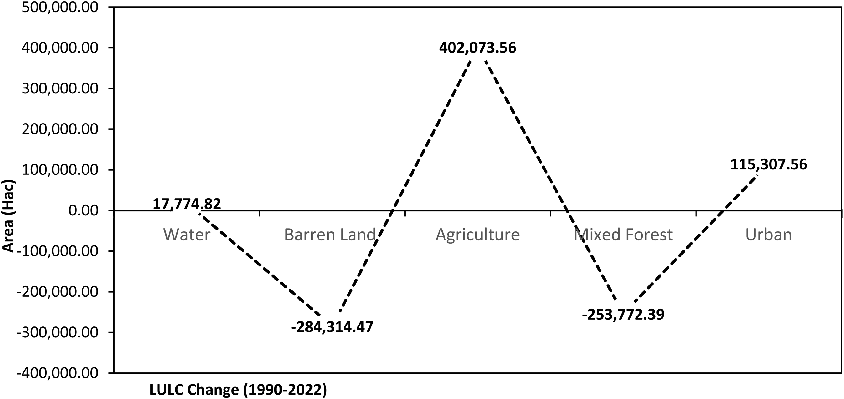
Land use land cover (LULC) change from 1990 to 2022. Note: Figures 4, 5, 6, and 7 are the graphical representations of the Table 3 values that were obtained from the classified images for each decade of the study area.

Figure 8.

Soil and Water Assessment tool (SWAT) model process framework of input and output data for the simulation, calibration, and validation of data.

Table 1.

Description of data.

Data information
Data	SOURCE	Description
DEM	(USGS) https://earthexplorer.usgs.gov/	30 × 30 m
LULC	(USGS) https://earthexplorer.usgs.gov/	30 × 30 m
Soil	(FAO,UN)https://www.fao.org/soils-portal/data-hub/soil-maps-and-databases/faounesco-soil-map-of-the-world/en/	Soil Properties and features
Weather Data	(NASA)https://power.larc.nasa.gov/data-access-viewer/	(WGEN)

Note: Table 1 includes data types and source information used for the study.USGS: United States Geographical Survey; FAO: Food and Agricultural Organization; NASA: National Aeronautics Space Administration; LULC: land use land cover; DEM: digital elevation model.

Table 2.

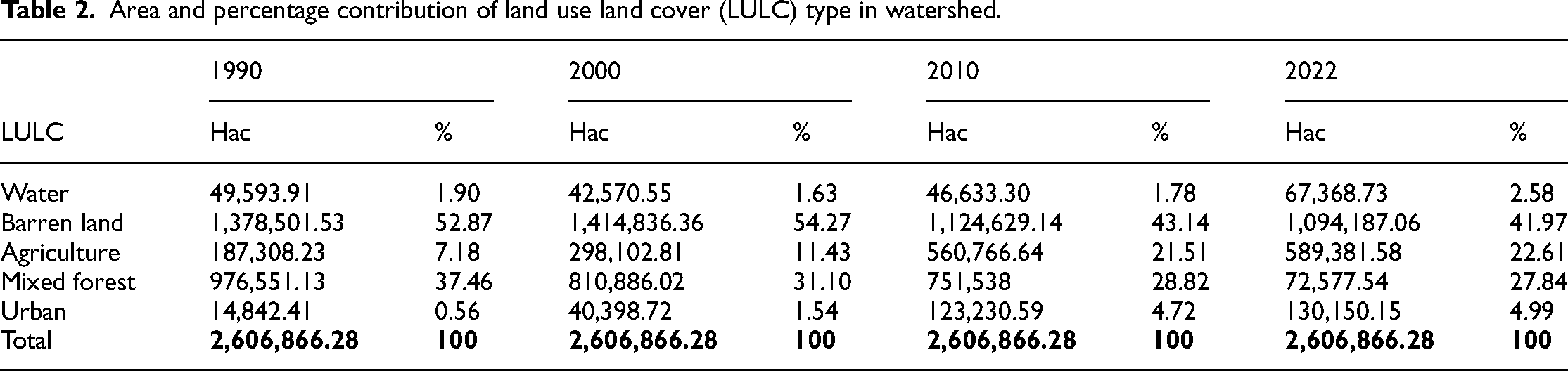
Area and percentage contribution of land use land cover (LULC) type in watershed.

LULC	1990		2000		2010		2022
LULC	Hac	%	Hac	%	Hac	%	Hac	%
Water	49,593.91	1.90	42,570.55	1.63	46,633.30	1.78	67,368.73	2.58
Barren land	1,378,501.53	52.87	1,414,836.36	54.27	1,124,629.14	43.14	1,094,187.06	41.97
Agriculture	187,308.23	7.18	298,102.81	11.43	560,766.64	21.51	589,381.58	22.61
Mixed forest	976,551.13	37.46	810,886.02	31.10	751,538	28.82	72,577.54	27.84
Urban	14,842.41	0.56	40,398.72	1.54	123,230.59	4.72	130,150.15	4.99
Total	2,606,866.28	100	2,606,866.28	100	2,606,866.28	100	2,606,866.28	100

Table 3.

Summary of land use land cover (LULC) change in watershed.

LULC	Area change		Area change		Area change		Area change		Annual rate of change (hac/y)
	(1990–2000)		(2000–2010)		(2010–2022)		(1990–2022)		Annual rate of change (hac/y)
	Hac	%	Hac	%	Hac	%	Hac	%
Water	−7023.36	−0.26	4062.75	0.15	20,735.43	0.79	17,774.82	0.68	423.21
Barren land	36,334.83	1.39	−290,207.22	−11.13	−30,442.08	−1.16	−284,314.47	−10.90	−6759.39
Agriculture	110,794.58	4.25	262,663.83	10.07	28,614.94	1.09	402,073.35	15.42	9573.17
Mixed forest	−165,665.11	−6.35	−59,348.02	−2.27	−25,759.26	−0.98	−253,772.39	−9.62	−6042.19
Urban	2556.31	0.98	82,832.59	3.17	6919.56	0.26	115,307.56	4.42	2745.21

Table 2 shows LULC contribution % in hectares within the watershed in each decade. The percent change was calculated using (MLC) classification values for each class.

Table 3 shows the area change of each LULC in hectares within the watershed. The area change value calculated using (MLC) classification values for each LULC class.

Description and setup of Soil and Water Assessment tool model

Model simulations are considered to be a more effective, functional tool,⁴³ to understand how LULC and climate change lead changes to hydrological cycle and sediment export.⁴⁴ The Soil and Water Assessment tool (SWAT) model is a semi-distributed, physically based, continuous model that simulates the hydrological process in small and large basins with high computational efficiency. SWAT is considered to be a very easy and user-friendly model, facilitating user the modification to acquire different hydrological components in the catchment. One of the most advantageous properties of the model is that it runs even at minimum data inputs and make easy and helpful for the regions that have limited data availability. Hence SWAT is considered to be more effective tool applied for the simulation of hydrological components in terms of HRU, including land use, soil type, and slope. The number of studies set the model to simulate surface runoff, interception storage, ground water flows, tile drainage, percolation, water quality nutrient, and sediment movement in hydrological process of watershed.⁴⁵ Several methods are involved to process the model. To estimate the surface runoff volume within the watershed, model uses the soil conservation services (SCS) approach under the examined change in land use and type of soil. The water is distributed in the number of forms, when surface runoff is generated. The water is distributed in the form of infiltration percolation of the soil profile that is stored by roots depending on the field capacity of the soil.²² The water balance equation consists of hydrological components is given in equation (vi) and water yield equation is given in equation (vii).

swt = sw 0 + \sum_{i = 1}^{t} (Rday + Qsur - Ea - Wseep - Qgw)

(6)

wyld = Qsur + Qlat + Qgw - Tloss

(7)where

s w t

indicates soil moisture content (mm),

s w 0

indicates soil moisture in the day

i

T

indicates time (days),

R d a y

indicates precipitation (mm) on the day

i

Q s u r

indicates surface runoff (mm) on the day

i

E a

indicates the evapotranspiration (mm) on the day

i

W s e e p

indicates moisture content (mm), entering the vedose zone from the soil profile on the day

i

Q g w

indicates return flow on the day

i

(mm),

T l o s s

indicates transmission loss (mm), and

Q l a t

indicates the lateral flow (mm).

For the estimation of sediment yield, SWAT employs the Modified Soil Universal Loss Equation, a modified version of Universal Soil Loss (USL) equation (citation). The equation is given as in equation (viii),

Sed = 11.8 (Qsur \times qp \times areaHRU)^{0.56} \times KUSLE \times CUSLE \times PUSLE \times LSUSLE \times CFRG

(8)where Sed indicates the sediment yield (tons), Qsur indicates the volume of surface runoff (mm-hac), qp indicates the rate of peak runoff (m³.s⁻¹), areaHRU indicates the hydrological response unit area (hac), KUSLE indicates soil erodibility factor, CUSLE indicates the factors of cover and management, PUSLE indicates the factor of support practice, LSUSLE indicates the topographic factors, CFRG indicates the coarse fragment fact. The flow diagram of SWAT model is given in Figure 8.

Indication of calibration and validation performance

In order to assess and evaluate the model performance, three evaluation metrics were used including NSE, root mean square error (RMSE), and R score. These matrices have specific properties of importance that help to understand forecasting model performance. Therefore, the selection of these metrics is based on future analysis, which helps to understand the model efficiently. These are defined as follows.

NSE: This indicator indicates the predictive ability of hydrological model. The most suitable value of NSE is 1. It ranges from −∞ to 1. It is given in equation (ix),

NSE = 1 \frac{\sum_{i = 1}^{T} (x i - y i) 2}{\sum_{i = 1}^{T} (x i - y i) 2}

(9)RMSE: When model uses observed values and predicted values, the average squared difference is found by using RMSE. It is important to find overall accuracy. If the value of RMSE is lowest, it indicates that model has performed effectively. It is given in equation (x),

RMSE = (y, x) = x = \sqrt{\frac{1}{T}} \sum_{i = 1}^{T} (y i - x i) 2

(10)R²: The correlation between two variables x and y is defined using R² metric. It is essential for model forecasting as help to assess and analyze the quality of the forecasting model.

Results and discussion

LULC changes over 4 decades

Comparing the change of LULC between 1990 and 2022 time span a significant change was found in the LULC. This time series was divided into a period of 10 years of change in LULC. For each land use land class the changes were calculated. Barren land, agriculture, and urban area increased by 1.39%, 4.25%, and 0.98%, respectively, while forest area decreased by 6.35% from 1990 to 2000. Agriculture and urban increased by 10.07%, and 3.17% respectively, while barren land and forest cover decreased by −11.13% and 2.27%, respectively from 2000 to 2010. During 2010–2022 agriculture increased by 1.09% and urban increased by 0.26%, while forest and barren land decreased by 0.98% and 1.16%, respectively. The overall change from 1990 to 2022 was found to have significant impacts on the hydrological components of the watershed including runoff generation, sediment yield, and water yield in both watershed and sub-watershed level. These changes were experienced due to increasing population which resulted urban and agriculture expansion, which decreased barren land and mixed forest ultimately from (1990–2022) as shown in graph (d). Economical interest also added agricultural expansion as the region is facilitated with rich soil and water available resources. The anthropogenic activities were the main reason to these changes.

Performance analysis

The performance of the model is evaluated by using the most important and widely used statistics Nash Sutcliffe, R Square, and RMSE. If NSE is zero, it is indicating the poor performance of the model, which means observed data is better indicator compared to the simulated data and, hence not acceptable. The relationship of variance is determined by the determination of coefficient. It ranges from 0 to 1. R² = 0 indicates poor performance of the model, R² = 1 indicates the best model performance. The indicator values given by model are given in Table 4 below:

Table 4.

Performance indicator values.

Performance indicator	Value
Root mean square error (RMSE)	12.78
NSE	0.99
R Square	0.89

The Figures 9 and 10 below show the calibration and validation of precipitation data.

Figure 9.

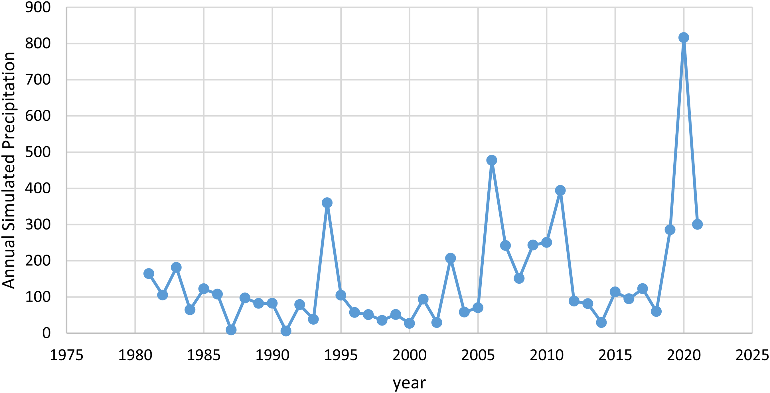
Showing annual simulated precipitation of Soil and Water Assessment tool (SWAT) model.

Figure 10.

Showing simulated and observed precipitation.

Sediment yield and water yield

(Zhu & Li, 2014)²⁰ showed the long-term impacts of LULC over change on the Tennesse River watershed suggested that expansion and development of urban areas are the main causes in terms of stream flow and runoff generation, forest expansion reduces the stream flow and surface runoff, while sediment and nutrient export is reduced by the reduction in agricultural areas. Li et al.,⁴⁶ stated that when land cover exceeds some threshold, the water yield is increased to a great extent. Yohannes et al.,⁴⁷ conducted study on the Blue Nile Basin in Ethiopia, stated that the area with the steeper slope exhibits the highest water yield and sediment yield, while the lower area of the watershed with low elevation and gentle slope exhibits low water yield and sediment yields. In our own conducted study we examined that the expansion in LULC class area of agriculture, urban area, and decrease in forest cover lead to the increase of sediment load in the catchment and runoff generation. The sub-basins with high elevation and slope, and less vegetation cover were prone to higher sediment load and showed a high water yield than the sub-basins with gentle slope and higher vegetation cover. The evaluated results of our study indicated that the sub-basins 11, 12, 13, and 14 were found to be more susceptible to the sediment load and water yield due to high elevation and slope. When comparing sub-basins 10, 4, and 1 to sub-basins 2, 3, 5, 6, 8, and 9, the basins 10, 4, and 1 contained high water yield availability. This may be caused because of differences in vegetation index, however were less susceptible to sediment load, when comparing to sub-basin 11, 12, 13, and 14. The average sediment export and water yield per year, and total sediment export and water yield in a decade for each sub-basin were quantified in each basin. The average sediment value for high elevated sub-basins 11, 12, 13, and 14 increased from 3.84 to 52, 3.79 to 43, 3.39 to 38, and 5.18 to 27.12(t/ha/y), respectively comparing the first decade (1981–1990) to last decade (2011–2022). On the other hand average sediment export value for sub-basins 1, 2, 3, 4, 5, 6, 7, 8, 9, and 10, was 0.37 to 10.82, 0.08 to 3.70, 0.80 to 25.44, 0.31 to 5.81, 0.13 to 5.37, 0.96 to 21.55, 0.06 to 3.06, 1.13 to 23.98, 0.13 to 2.74, 0.31 to 4.42 (t/ha/y), respectively comparing decade (1981–1990) to (2011–2022). The average water yield for sub-basins 11, 12, 13, and 14 showed an increase of 13.57 to 149.67, 13.29 to 147.52, 16.64 to 139.55, and 23.39 to 130.50, respectively (mm/y) comparing the first decade (1981–1990) to the last decade (2011–2000). While water yield values for sub-basins 1, 2, 3, 4, 5, 6, 7, 8, 9, and 10 changed as 9.73 to 180.56, 2.12 to 101.48, 3.18 to 143.03, 9.51 to 150.04, 2.95 to 108.77, 4.04 to 114.18, 1.97 to 101.53, 4.20 to 114.11, 2.54 to 111.00, and 14.15 to 156.08, respectively from 1981 to 1990 to 2011 to 2022. The average sediment export per year in a decade is given in Table 5, while Figure 11 represents the total sediment export change in each decade. Similarly, Table 6 represents the average water yield per year in a decade and Figure 12 represents the total water yield Change in each decade on the sub-basin level.

Figure 11.

Showing temporal evolution of total simulated sediment export distribution (1981–2022).

Figure 12.

Showing temporal evolution of total simulated water yield distribution (1981–2022).

Figure 13.

Total SRQ, PCP, WYLD, SYLD in each decade (1981–2022). SRQ: surface runoff; PCP: precipitation; WYLD: water yield; SYLD: sediment yield.

Table 5.

Average sediment export per year in a decade in each sub-basin.

Sub-basin	Average sediment export (ton/hac/y) (1981–1990)	Average sediment export (ton/hac/y) (1991–2000)	Average sediment export (ton/hac/y) (2001–2010)	Average sediment export (ton/hac/y) (2011–2022)
1	0.37	0.48	0.41	10.82
2	0.08	0.17	0.05	3.70
3	0.80	0.6	0.54	25.44
4	0.31	0.57	0.31	5.81
5	0.13	0.33	0.1	5.37
6	0.96	1.86	0.68	21.55
7	0.06	0.16	0.07	3.06
8	1.13	2.11	0.77	23.98
9	0.13	0.41	0.12	2.74
10	0.31	0.54	0.35	4.42
11	3.84	5.15	3.48	52.17
12	3.79	5.75	4.06	43.69
13	3.39	5.52	4.37	38.28
14	5.18	4.15	14.07	27.12

Table 6.

Average water yield per year in a decade in each sub-basin.

Sub-basin	Average water yield-mm (1981–1990)	Average water yield-mm (1991–2000)	Average water yield-mm (2001–2010)	Average water yield-mm (2011–2022)
1	9.73	10.59	6.25	180.56
2	2.12	4.94	1.45	101.48
3	3.18	3.37	2.04	143.03
4	9.51	14.54	6.77	150.04
5	2.95	5.86	2.17	108.77
6	4.04	8.23	3.00	114.18
7	1.97	4.47	1.56	101.53
8	4.20	8.10	2.79	114.11
9	2.54	8.97	2.75	111.00
10	14.15	20.47	9.70	156.08
11	13.57	18.64	11.75	149.67
12	13.29	18.85	12.09	147.52
13	16.64	23.06	20.02	139.55
14	23.39	19.88	59.37	130.50

The change in precipitation, water yield, sedimen export, and surface runoff

The change in precipitation, water yield, sediment load, and surface runoff in each decade is shown in the graph below. This graph indicates the changes in each component in each decade on basin level. The average change per year in each component was calculated as, precipitation (792.74 mm), sediment load (71.73 ton/hac), water yield (499.12), and surface runoff (467.36 mm). Figure shows the simulated change in each variable.

As shown in Figures 14, 15, and 16. The continuous change in precipitation in the future leading to change in both of the hydrological components (water yield and sediment export). Figures 14 15, and 16 show the results that have been evaluated for future predictions

Figure 14.

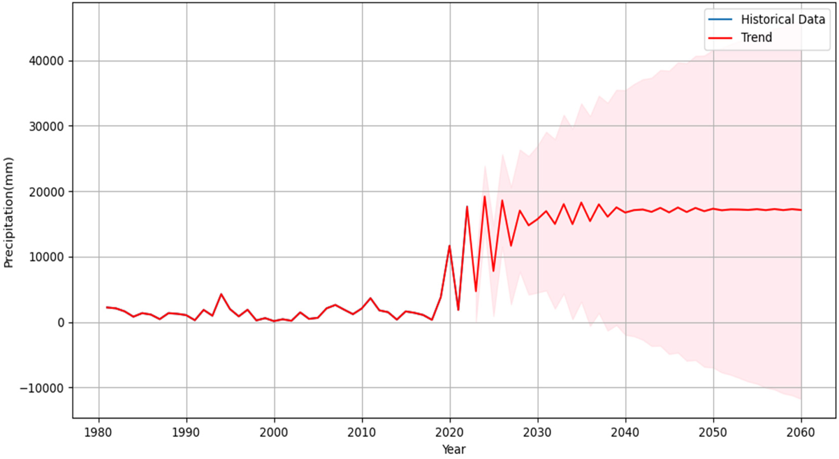
Showing prediction of precipitation using autoregressive integrated moving average (ARIMA) model.

Figure 15.

Showing prediction of sediment load in the catchment using seasonal autoregressive integrated moving average with exogenous factors (SARIMAX) model.

Figure 16.

Showing prediction of water yield in the catchment using seasonal autoregressive integrated moving average with exogenous factors (SARIMAX) model.

Limitations of the study

The study evaluated change in precipitation trend, water yield, and Sediment export and runoff generation in the watershed on basin and sub-basin level. These changes were of importance to find the actual reasons and factors. Hence our study focuses the two most important factors LULC change and climate variability into the watershed using LULC imagery datasets and weather datasets. The main problem limited availability of observed data in such a huge watershed. This study almost solely relied on precipitation and simulated data due to non-available data resources, however our results for precipitation data are reliable and acceptable, which is the base to train our machine models. Despite all these observations and results, it is much more important to address these limitations by proper measurement and maintained documentation by installing gauge stations in such a large watershed.

Conclusion

Our study aimed to analyze the spatio-temporal changes in LULC and climate variability, leading to change in hydrological processes in the most important watershed of the region using SWAT model. The study found the ultimate change in main LULC classes, including an increase in urban area, and agriculture, and decline in barren land and mixed-forest are leading to change in precipitation patterns, and hydrological components. This is indicating an unbalanced environment within the watershed. Such an increase in runoff generation and sediment load will affect the agriculture and water available resources. In addition, phosphorus carried by sediment load will cause water quality problems. Therefore study recommends management of the LULC in the watershed to sustain agriculture and to maintain sediment load by maintaining runoff generation to avoid present and future challenges.

Footnotes

Acknowledgements

The authors extend gratitude to the Centre for Environmental Science, University of Sindh Jamshoro, Sindh, Pakistan for their support during the research project.

Author contribution

Rabia Chhachhar contributed to the conception and design, data collection, interpretation, analysis, visualization, writing original draft, reviewing manuscript. Habibullah Abbasi contributed to the conception and design, interpretation, analysis, writing, editing, and reviewing all drafts. The Authors worked in collaboration and approved the final manuscript.

Data availability

Data for this study is available from the corresponding author upon reasonable request.

Declaration of conflicting interests

The authors declared no potential conflicts of interest with respect to the research, authorship, and/or publication of this article.

Funding

The authors received no financial support for the research, authorship, and/or publication of this article.

Preprint DOI

Chhachhar R, Abbasi H. Hydrological Response to Land Use Land Cover and Climate Variability, and Simulation of Sediment Export and Water Yield in the Catchment Kotri Sindh Pakistan Using SWAT Model.; 2023. doi:10.22541/au.169999221.18673873/v1

ORCID iD

Rabia Chhachhar

Author biographies

Rabia Chhachhar is a graduate student from the Centre for Environmental Science, University of Sindh Jamshoro, Pakistan. Her research focuses on GIS Modeling and GIS analysis in the field of Hydrology and Climate change leading to a change in hydrological behavior. Her research dedication is to GIS-based Environmental decision-making for sustainability goals

Habibullah Abbasi is a professor in the Department of Centre for Environmental Science, faculty of Natural Science, University of Sindh Jamshoro. He previously worked as Assistant professor in Energy & Environment Engineering Department, Quaid – e – Awam University Nawabshah, visiting scholar in Center for Environmental Sciences, University of Sindh, Jamshoro, Pakistan, and as Assistant professor, Environmental Sciences Sindh Madressatul Islam University Karachi. He has worked for different publication journals as an author and reviewer. His research interest include Atmospheric Environment, Interpretation of Earth's surface by satellites to find out effective ways to monitor global and regional changes on Earth surface, including the application of Climate and Environmental modeling.

References

Garg

Nikam

Thakur

, et al. Human-induced land use land cover change and its impact on hydrology. HydroResearch 2019; 1: 48–56.

Bosch

Hewlett

. A review of catchment experiments to determine the effect of vegetation changes on water yield and evapotranspiration. J Hydrol 1982; 55: 3–23.

Gashaw

Tulu

Argaw

, et al. Modeling the hydrological impacts of land use/land cover changes in the Andassa watershed, Blue Nile Basin, Ethiopia. Sci Total Environ 2018; 619: 1394–1408.

Wang

Kalin

Kuang

, et al. Individual and combined effects of land use/cover and climate change on Wolf Bay watershed streamflow in southern Alabama. Hydrol Processes 2014; 28: 5530–5546.

Gemechu

Zhao

Bao

, et al. Estimation of hydrological components under current and future climate scenarios in guder catchment, upper Abbay Basin, Ethiopia, using the SWAT. Sustainability 2021; 13: 9689.

Luo

Liu

Meng

, et al. Identifying climate change impacts on water resources in Xinjiang, China. Sci Total Environ 2019; 676: 613–626.

Mitiku

Meresa

Mulu

, et al. Examining the impacts of climate variabilities and land use change on hydrological responses of Awash River basin, Ethiopia. HydroResearch 2023; 6: 16–28.

Woldemichael

Hossain

Pielke Sr

. Evaluation of surface properties and atmospheric disturbances caused by post-dam alterations of land use/land cover. Hydrol Earth Syst Sci 2014; 18: 3711–3732.

Warburton

Schulze

Jewitt

. Hydrological impacts of land use change in three diverse South African catchments. J Hydrol 2012; 414: 118–135.

10.

Falkenmark

Andersson

Castansson

, et al. Water a reflection of land use: options for counteracting land and water mismanagement. Stockolm,(Sweden): Swedish Natural Science Council NFR, 1999.

11.

Swain

Mishra

Pandey

, et al. Hydrological modelling through SWAT over a Himalayan catchment using high-resolution geospatial inputs. Environ Chall 2022; 8: 100579.

12.

Mundetia

Sharma

, et al. Assessment of hydrological response with an integrated approach of climate, land, and water for sustainable water resources in the Khari River basin, India. Anthropocene 2023; 41: 100373.

13.

Gebre

Getahun

Fufa

, et al. Hydrological responses of land use land cover change on the Hangar catchment, Blue Nile Basin. Published online 2022.

14.

Birhanu

Moges

Sinshaw

, et al. Hydrological modeling, impact of land-use and land-cover change on hydrological process and sediment yield; case study in Jedeb and Chemoga watersheds. Energy Nexus 2022; 5: 100051.

15.

Chang

Johnson

Hinkley

, et al. Spatial analysis of annual runoff ratios and their variability across the contiguous US. J Hydrol 2014; 511: 387–402.

16.

Welde

Gebremariam

. Effect of land use land cover dynamics on hydrological response of watershed: case study of Tekeze dam watershed, northern Ethiopia. Int Soil Water Conserv Res 2017; 5: 1–16.

17.

Esse

Ríos

Saavedra

, et al. Effects of land use change on water availability and water efficiency in the temperate basins of south-central Chile. J King Saud Univ Sci 2021; 33: 101650.

18.

Anand

Gosain

Khosa

. Prediction of land use changes based on land change modeler and attribution of changes in the water balance of Ganga basin to land use change using the SWAT model. Sci Total Environ 2018; 644: 503–519.

19.

Mangi

Onywere

Kitur

, et al. Hydrological response to land use and land cover change on the slopes of Kilimanjaro and Meru mountains. Ecohydrol Hydrobiol 2022; 22: 609–626.

20.

Zhu

. Long-term hydrological impacts of land use/land cover change from 1984 to 2010 in the Little River Watershed, Tennessee. Int Soil Water Conserv Res 2014; 2: 11–21.

21.

Serrão EA

Silva

Ferreira

, et al. Impacts of land use and land cover changes on hydrological processes and sediment yield determined using the SWAT model. Int J Sediment Res 2022; 37: 54–69.

22.

Liu

Fan

, et al. Hydrological impacts of land use/cover changes in the Lake Victoria basin. Ecol Indic 2022; 145: 109580.

23.

Bal

Dandpat

Naik

. Hydrological modeling with respect to impact of land-use and land-cover change on the runoff dynamics in Budhabalanga river basing using ArcGIS and SWAT model. Remote Sens Appl: Soc Environ 2021; 23: 100527.

24.

Chaves

Neill

Germer

, et al. Land management impacts on runoff sources in small Amazon watersheds. Hydrol Process 2008; 22: 1766–1775.

25.

Gyamfi

Ndambuki

Salim

. Hydrological responses to land use/cover changes in the Olifants Basin, South Africa. Water (Basel) 2016; 8: 588.

26.

Juma

Nkongolo

Raude

, et al. Assessment of hydrological water balance in Lower Nzoia Sub-catchment using SWAT-model: towards improved water governace in Kenya. Heliyon 2022; 8.

27.

Xiao

Wang

. Impacts of land use/land cover and climate change on hydrological cycle in the Xiaoxingkai Lake Basin. J Hydrol Reg Stud 2023; 47: 101422.

28.

Nie

, et al. Assessing-impacts-of-Landuse-and-Landcover-changes. 2011.

29.

Barkey

Mappiasse

Nursaputra

. Model of climate and LAND-USE changes impact on water security in Ambon city, Indonesia. J Geomat Plan 2017; 4: 97–108.

30.

Giri

Arbab

Lathrop

. Assessing the potential impacts of climate and land use change on water fluxes and sediment transport in a loosely coupled system. J Hydrol 2019; 577: 123955.

31.

Brath

Montanari

Toth

. Analysis of the effects of different scenarios of historical data availability on the calibration of a spatially-distributed hydrological model. J Hydrol 2004; 291: 232–253.

32.

Dodov

Foufoula-Georgiou

. Incorporating the spatio-temporal distribution of rainfall and basin geomorphology into nonlinear analyses of streamflow dynamics. Adv Water Res 2005; 28: 711–728. A.

33.

Kampata

Parida

Moalafhi

. Trend analysis of rainfall in the headstreams of the Zambezi River Basin in Zambia. Phys Chem Earth, Parts A/B/C 2008; 33: 621–625.

34.

Gajbhiye

Meshram

Singh

, et al. Precipitation trend analysis of Sindh River basin, India, from 102-year record (1901–2002). Atmos Sci Lett 2016; 17: 71–77.

35.

Sayemuzzaman

Jha

. Seasonal and annual precipitation time series trend analysis in North Carolina, United States. Atmos Res 2014; 137: 183–194.

36.

Priyan

. Spatial and temporal variability of rainfall in Anand District of Gujarat State. Aquatic Proc 2015; 4: 713–720.

37.

Narayanan

Basistha

Sarkar

, et al. Trend analysis and ARIMA modelling of pre-monsoon rainfall data for western India. CR Geosci 2013; 345: 22–27.

38.

Latif

Hazrin

NAB

Koo

, et al. Assessing rainfall prediction models: exploring the advantages of machine learning and remote sensing approaches. Alexandria Eng J 2023; 82: 16–25.

39.

Ali

. Time series analysis of Baghdad rainfall using ARIMA method. Iraqi J Sci 2013; 54: 1136–1142.

40.

Tumsa

Kenea

Tola

. The application of SWAT+ model to quantify the impacts of sensitive LULC changes on water balance in Guder catchment, Oromia, Ethiopia. Heliyon 2022; 8.

41.

Congedo

. Semi-automatic classification plugin documentation. Release 2016; 4: 29.

42.

Lillesand

Kiefer

Chipman

. Remote sensing and image interpretation. John Wiley & Sons, 2015.

43.

Woznicki

Nejadhashemi

Tang

, et al. Large-scale climate change vulnerability assessment of stream health. Ecol Indic 2016; 69: 578–594.

44.

Giri

Nejadhashemi

Zhang

, et al. Integrating statistical and hydrological models to identify implementation sites for agricultural conservation practices. Environ Model Softw 2015; 72: 327–340.

45.

Serur

Adi

. Multi-site calibration of hydrological model and the response of water balance components to land use land cover change in a rift valley Lake Basin in Ethiopia. Scientific African 2022; 15: e01093.

46.

Ramankutty

Coe

. Modeling_the_Hydrological_Impact_of_Land-use_Chang.

47.

Yohannes

Soromessa

Argaw

, et al. Impact of landscape pattern changes on hydrological ecosystem services in the Beressa watershed of the Blue Nile Basin in Ethiopia. Sci Total Environ 2021; 793: 148559.

Hydrological response to land use land cover and climate variability,and simulation of sediment export and water yield in the catchment Kotri Sindh Pakistan using Soil and Water Assessment tool model

Abstract

Keywords

Introduction

Material and methods

Study area description

Data collection

Predicting rainfall, sediment yield, and water yield

Machine learning and predictive models

ARIMA model, and SARIMAX model

Multi-temporal analysis of land cover change

Description of change in LULC classes

Description and setup of Soil and Water Assessment tool model

Indication of calibration and validation performance

Results and discussion

LULC changes over 4 decades

Performance analysis

Sediment yield and water yield

The change in precipitation, water yield, sedimen export, and surface runoff

Limitations of the study

Conclusion

Footnotes

Acknowledgements

Author contribution

Data availability

Declaration of conflicting interests

Funding

Preprint DOI

ORCID iD

Author biographies

References