Sage Journals: Discover world-class research

Abstract

Accurate modeling of viral outbreaks in living populations and computer networks is a prominent research field. Many researchers are in search for simple and realistic models to manage preventive resources and implement effective measures against hazardous circumstances. The ongoing Covid-19 pandemic has revealed the fact about deficiencies in health resource planning of some countries having relatively high case count and death toll. A unique epidemic model incorporating stochastic processes and queuing theory is presented, which was evaluated by computer simulation using pre-processed data obtained from an urban clinic providing family health services. Covid-19 data from a local corona-center was used as the initial model parameters (e.g. $R_{0}$ , infection rate, local population size, number of contacts with infected individuals, and recovery rate). A long–run trend analysis for 1 year was simulated. The results fit well to the current case data of the sample corona center. Effective preventive and reactive resource planning basically depends on accurately designed models, tools, and techniques needed for the prediction of feature threats, risks, and mitigation costs. In order to sufficiently analyze the transmission and recovery dynamics of epidemics it is important to choose concise mathematical models. Hence, a unique stochastic modeling approach tied to queueing theory and computer simulation has been chosen. The methods used here can also serve as a guidance for accurate modeling and classification of stages (or compartments) of epidemics in general.

Keywords

Epidemiology stochastic modeling queueing simulation epidemic stage classification

Introduction

Main objective of this work is to provide a simplified guide for building models that cover all the stages of an epidemic outbreak. Due to the discrete nature of its elements, epidemiology contains several randomness. This fact encourages us to model events of epidemiology as stochastic processes in order to increase the accuracy of the model at hand. The model presented here is not only eligible for producing reliable results, it also provides analysis of future tendencies. Another unique contribution of this paper is the formulation of the state transitions of the stages of an epidemic: (a) from healthy to susceptible, (b) from susceptible to infected, (c) from infected to quarantined, (d) from quarantined to recovered, and (e) from recovered to healthy. Furthermore, efficiency analysis of the recovery process dealing with different service/qualities is also discussed.

We do not specifically discuss the characteristics of some known approaches, for example, deterministic and stochastic approaches. We intended to design a more generic model, which can be applied to building models for human epidemics and computer epidemics with minor modifications. The approach presented here is based on stochastic processes and queueing theory. Stochasticity possessed inherently by epidemiology, and flexibility of applying stochastic models to a wide area of sciences encourages us to choose this approach for modeling epidemics on human and computer networks.

We computer engineers and medical doctor have limited knowledge of stochastic processes and queueing theory, which provide valuable methods and techniques for modeling stochastic systems. We usually describe event dynamics using models that are formalized mathematically. Although, inevitable, rigid mathematical formalization can sometimes be cumbersome and/or even disruptive when applying to experimentation and system implementation. There are, naturally, cases where complex theoretical proofs are necessary. However, there also exist areas of science that have already been discussed widely using a multitude of theories and their proofs. To obtain maximum benefit from the material presented here, we intend to simplify mathematical presentations and avoid theoretical proofs so that the models and approaches given can be easily adapted to various purposes, for example, experimentation, simulation, and resource management.

As detailed in Kondakci and Dincer,¹ lifecycle of an epidemic system generally consists of five stages, healthy, susceptible, infected, quarantined, and recovered. These are modeled as distinct states taking place in a chain of interrelated stochastic processes. The states are in most cases recurrent, omitting the case of death (an absorbing state). In any case, an infection case goes dynamically through certain transitive states, that is, moving from one state to another. Each state is numerically described either by a probabilistic function or by an integer count. The probabilistic function represents the probability of estimating the value of a given parameter, for example, probability of being infected among 100 susceptible individuals. Or, it can also describe the probability of being in a state, for example, probability of being recovered within a specific time duration. A state can also be represented by the number of increments/decrements in sizes of a parameter, for example, infected population size, the state of infectious patients undergoing quarantine operations, and the number of recovered patients.

To estimate related parameters, we generally build mathematical models fitted to some data set. Unfortunately, this is more difficult than it sounds. Because errors in statistical fitting and uncertainty in the parameter estimations are inevitable.² Epidemiology is often limited to the study of disease spreading in populations of humans or animals. Several commonalities between the human and computer epidemiology have recently emerged. In order to gain a general perspective, we consider that computer worms/viruses (malware) and epidemic threats to living populations (human, animal) are interchangeable. Therefore, assuming readers are from multidisciplinary environments, we avoid complex mathematical manipulations and in-depth proofs of theories, and instead focus on the applicability and correctness of the presented models. The aim is thus to provide a set of general formulae and methods that can be easily adapted to special cases in order to perform realistic trend analysis in epidemics. Simulations and experimental analysis of various cases will then be facilitated by simply modifying the general model provided.

We use stochastic approaches in conjunction with queueing theory to analyze the stages of epidemic outbreaks. Models discussed are generally substantiated by simulations and numerical examples, some of which are given here. If needed, one can refer to Taha³ and Medhi⁴ for a comprehensive coverage of Operations Research and Stochastic Models in Queueing Theory, and Cui et al.⁵ for Markov models used in a multi-state repairable systems.

Motivations and related work

In–depth study of epidemiology is an extremely complex area of research. Contemporary infectious diseases evolve sporadically across a wide spectrum, for example, Covid-19 pandemics,^6–8 and fundamental concepts requiring detailed study are infection spread, surveillance, treatment, control, immunity in populations, and resource management. With the Covid-19 pandemics, the world has realized the importance of the efficient resource management for health institutions, where most countries have shown significant deficiencies in their health systems. For instance, even though it has relatively efficient health system, Turkey has locked down all the polyclinics of the major hospitals throughout the country and mobilized the resources to thwart the pandemics.

So called Recurrent Epidemic Model (REM) first introduced, by Kondakci and Dincer,¹ applies a comprehensive stochastic analysis to computer epidemics, processing through a detailed analysis of a five stage stochastic model, where each stage is mathematically explored to obtain a satisfactory formalism in all dominating stages in the epidemiology. REM presents an extended structure of state transitions in order to highlight the shortcomings of the classical and deterministic models. It aims to obtain higher accuracy by use of a comprehensive model containing a sequence of stochastically dependent compartments. Other interesting approaches have been discussed in Amador and Artalejo,^9,10 Yang et al.,¹¹ and Sellke et al.¹² An epidemic model,¹³ applying the finite-Markovian process gives an overview of the steady-state analysis of the evolution of an epidemic case¹³ has proposed concrete solutions for determining transition dynamics by formalizing the parameters for the infection and recovery rates.

Additionally,¹⁴ discusses the detection of worm spread, with suffeciently detailed deterministic and stochastic models. Several stochastic approaches have also been proposed to analyze dynamics of epidemics, for example, Ortega et al.¹⁵ To gain an insight into the stochastic models, the reader can examie the survey on stochastic epidemic models presented in Britton.¹⁶ Mathematics and simulation are effective tools assisting us in almost every field of research, in particular, for building models and substantiating the model results with regard to the theoretical background. A review of mathematical models dealing with malware propagation in computer networks is presented in del Rey.¹⁷

Classical epidemic models (e.g. SIR, SIS, SEIR) maintain their relevance within the field of epidemic research, providing a simpler and more structural overview of epidemic outbreaks. Related to this, Artalejo and Lopez-Herrero¹⁸ discusses the dynamics of susceptible-infective-removed (SIR) model with the aid of continuous time Markov chains. A cellular automata based SEIR model for computer virus spreading is proposed in Batista et al.¹⁹ A stochastic approach of analysis covering SIR models is considered in Kenah and Robins.²⁰

Several important characteristics are common to almost all fields of research, such as mathematical biology, computer science, physics, economics, and the socail science.²¹ Therefore, it is hard to confine epidemiology research to a particular field, without restricting the methods used to analyze cases that can lead to inaccurate results. For example, Mukhopadhyay and Bhattacharyya²² discusses a comprehensive mathematical model considering the propagation of infections in human populations, which applies the theory of (traveling) waves to build the epidemic model. A comprehensive study of the mathematical epidemiology containing several models is presented in Hethcote.²³ Other interesting models can be found in Paul and Mishra,²⁴ Ren et al.,²⁵ Kudo et al.,²⁶ and Wanget al.²⁷

A computer worm is an intelligent virus that can automatically spread through vulnerable (or unprotected) computer applications. Some protection systems are incapable of detecting certain viruses, which are classified as polymorphic viruses, such as Stuxnet.²⁸ Worms are often deployed en–mass by mass–mailing in order to cause system unavailability.²⁹ A survey on taxonomy and characterization of computer worms is presented in Fachkha and Debbabi.³⁰ Numerous computer worm models exist in the literature, most of which are rooted in the classical biological models.^31–34

It is also important to study the efficiency of quarantine strategies under various infection profiles. To do so, we need to have an additional stage (compartment) dealing with modeling of the quarantine process. This paper deals with a stochastic model with five compartments progressing from the healthy state to the recovered state in order to cover all the major stages in general. Effect of the incubation time on the transmission of the p. vivax malaria is discussed in Nah et al.³⁵

As also discussed in Kondakci,¹³ many solutions assume homogeneous systems with constant transition rates, where states change with invariant probabilities. However, it has been frequently observed that both the threatened objects and their responses are heterogeneous, where states change with varying probabilities.

Communication patterns in a network is important for the propagation of viral infections. For example, the total number of bites made by mosquitoes has an important impact on the incubation time and transmission probability of malaria.³⁶ Immunization is naturally an important part during the course of an epidemic spreading. Accordingly, Pastor-Satorras and Vespignani³⁷ considers epidemics and immunization in scale–free networks applying a rigid mathematical analysis. Scale–free networks related to epidemic dynamics is considered in Fu et al.³⁸ Network traffic characteristics for some computer viruses may not be as important as we assume. Regarding this, Sharif et al.³⁹ discusses some approaches used in computer epidemics to generate propagation methods that result in successful worm outbreaks, ignoring the traffic characteristics of networks.

Models that do not incorporate the incubation period, and assume only deterministic distributions of the compartmental parameters and state changes will generally fail when fitting data to the initial outbreak data.

Susceptible nodes do not have latent periods. Since the infection cases behave differently regarding the population and infection types, the related model must accommodate the evolution of each specific case. The model presented in Kondakci and Dincer¹ discusses methods to overcome the limitations by introducing additional parameters to model the incubation periods.

For example, incubation period of computer viruses generally depends on the deployment of the individual virus and the immunity (or protection level) of the victim system. Assuming a malcode (virus, worm, trojan) embedded in an e-mail attachment, and the victims (users) of the receiving host delay opening the malcoded attachments, then the latent time might eventually be very long. Some aggressive worms like the well-known CodeRedII⁴⁰ worm, W32.Goner.A@mm, and SQL–Slammer⁴¹ may immediately infect systems (zero latent time) without sufficient protection.

Population structures

Epidemic analysis deals with interrelated classes of populations from different networks, where the elements of each network are subject to different treatments in different stages during the course of an epidemic case. Two different types of networks are considered here, centralized and scale–free networks. Nodes in a scale–free network are connected through short paths, where the number of connections emanating from a given object obeys the power-law distribution. In epidemiology, “short path” means that the connectivity weight of two neighboring nodes is reasonably short, or the frequency of contact is sufficient to cause an infection, and therefore proper control of the epidemic spread requires more effort and resources. In contrast to scale–free networks, centralized networks have low degree of connectivity among the nodes, that is, fewer number of individuals in a population. Hence, regarding the epidemiology, nodes in a centralized networks have low rate of infection compared to the scale–free networks.

Centralized networks

Centralized networks are those that encompass many elements with low degree of connectivity. Typically, human epidemiology from small-sized communities exhibits the characteristics of centralized networks, because connectivity factors among the individuals are small and the epidemic spread is more under the control of individuals. Humans’ inherent intelligence under many circumstances can limit their access to the pathogenic environment. There are also exceptional populations who are unable to contact, for example, military wards, jails, mass production plants, complex residential areas, farms, and animal flocks. Thus, a parameter denoting the degree of contact for such networks has a significant role in the epidemiology of dense networks (e.g. intensely crowded populations).

Scale-free networks

Scale-free networks (SFN) are those that follow the properties of the power low distribution, where there is an exponential relation between the degree of connectivity of a node and the frequency of connections it makes. More on discussions about power low can be found in Newman.⁴² Scale-free networks are regularly present in all forms of networks such as computer networks, social networks, and biological systems. SFNs have the property of power law, where a quantity changes as a power of another, that is, $P (k) = k^{- γ}$ , which denotes a tight relationship between two variables, where a change in one causes a change in the other. The changes are mutual, relatively proportional, and independent of the initial conditions. For example, the probability that an infectious node contacts $k$ susceptible hosts obeys the power-law distribution as $P (k) = k^{- 2.06}$ . Unfortunately, analysis and characterization of power-law data is very complex; least-square fitting method is often used to analyze the power low data, which usually leads to uncertainty and inaccuracy in the results. Therefore, it is important to apply a through statistical analyses on the empirical data in order to recognize its actual characteristics, and whether it accurately fits the power-law distribution. A statistical framework applying the method of maximum-likelihood fitting with the Kolmogorov–Smirnov statistics is used in Clauset et al.⁴³ for discriminating power-law patterns in some empirical data.

The power low property is also associated with preferential attachment, which refers to the distribution of properties among the nodes in a network. Scale-free networks generally grow progressively by randomly joined nodes, where each node links to current hosts with preferential attachment. That is, the probability of connecting to host $i$ is proportional to the number of currently connected links $k_{i}$ that host $i$ connected to Barabási,⁴⁴ that is,

P (joining node i) = \frac{k_{i}}{\sum_{j} k_{j}} .

For example, distribution of resources in a society will often centralize at a node with a higher degree of connections. A typical example of this is business people’s preference for commercials on highly attractive environments (e.g. TV channels, newspapers, or Web sites). Another example is the prevalence of malware attacks on highly connected computer networks in order to gain access to greater numbers of computers. Lower immunity facilitates the “invitation” of infectious diseases.

The rate of an infection a node undergoes depends on the number of contacts with infected nodes that it may have, as well as with the duration (or frequency) of the contacts. Assuming that each contact has the same infection rate denoted by $β$ , then the rate at which a node from the susceptible group $i$ gets infected is given by

λ = β \sum_{j}^{N} C_{i, j} I_{j},

(1)

where $I_{j}$ is the proportion of infectious nodes in population $j$ , $C_{i, j}$ denotes the number of contacts per time slot each node in group $i$ contacts nodes in population $j$ having the size of $N$ .

Growth and extinction dynamics

Let us consider the classical SIR (Kermack–McKendrick model³²) model and expand it to contain the dynamics of healthy $h (t)$ and quarantined $q (t)$ compartments. With this expanded SIR model (ESIR), we can explore significant details about the long-run dynamics of the state transitions of the system. Given the total number of nodes, $N (t)$ , at time $t$ , the number of healthy nodes is determined by summing the respective fractions from all compartments as

h (t) = N (t) - [s (t) + i (t) + q (t) + r (t)],

(2)

where $s (t)$ denotes the number of susceptible, $i (t)$ infected, $q (t)$ quarantined, and $r (t)$ recovered (removed) nodes. The fallowing differential equation set, equation (3), represents the dynamic behavior of the ESIR model.

\begin{matrix} Healthy : \frac{d}{dt} h (t) = φ N (t) - δ h (t) + μ r (t) + ε s (t) \\ Susceptible : \frac{d}{dt} s (t) = δ h (t) + ϵ_{s} r (t) - λ s (t) - ε s (t) \\ Infected : \frac{d}{dt} i (t) = λ s (t) - α i (t), \\ Quarantined : \frac{d}{dt} q (t) = α i (t) - γ q (t), \\ Recovered : \frac{d}{dt} r (t) = γ q (t) - μ r (t) . \end{matrix}

(3)

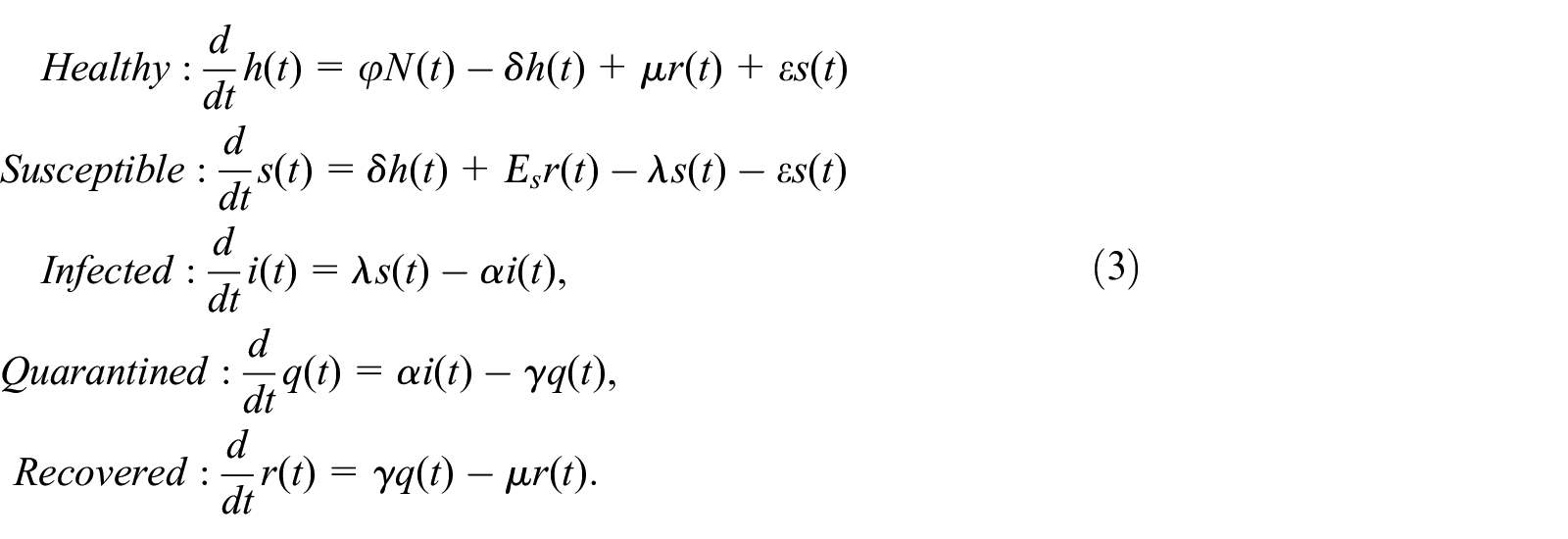
The parameters are self explanatory, for example, population change in a compartment is interrelated with the parameters of its predecessor and ancestor compartments. For example at time $t$ , the growth rate of the infected population i(t) depends on the number of the susceptible objects by a factor of $λ$ and the current size of the susceptible population $s (t)$ , minus the number of nodes removed from the infected population to the quarantine population $q (t)$ having the rate $γ$ , that is, $γ q (t)$ .

A distinct property of the ESIR model is that a very small proportion, $ϵ_{s} r (t)$ , of the repaired hosts that will be moved to the healthy population may again become susceptible. This can be considered as a loose user vigilance or degraded immunity due to lack of vaccination.

Basic reproduction number

The concept of basic regeneration number was first used in conjunction with demography in 1880s to predict the growth rate in specific sections of populations.⁴⁵ Regarding the epidemiology, it expresses the number of potential transmissions from a single infected node during its transmitter period, and is denoted by $R_{0}$ , meaning an offspring that starts at its first birth ( $0$ ) and reproduces itself with rate $R_{0}$ in time. There is no fixed formula for $R_{0}$ , which varies considerably from case to case, and even from population to population, taking on different parameters. Therefore, it is generally difficult to match its theoretical form to its practical use. In its simplest form, it is defined as a function of three parameters as

R_{0} = 〈 β, λ, μ 〉 .

Where, $β$ denotes the effective contact rate (i.e. efficacy of infection), $λ$ infection, and $μ$ recovery rate. We can then search for the changes in the parameters that lead endemic equilibrium, where the infection is constantly maintained with reproduction period of the disease.

There exist numerous methods to define $R_{0}$ , however which of these is the most accurate and applicable to a given case is frequently disputed by researchers. However, there is no doubt that $R_{0}$ has a remarkable role during the initial phase of epidemic spreading. As a quick reference, one can refer to Driessche and Watmough⁴⁶ for an elaborated work on the basic reproduction number, used in compartmental infection models. A preliminary estimation of $R_{0}$ of the novel Coronavirus (sars-cov-2) is presented in Zhao et al.⁴⁷ Considering varies categories of hosts, it is claimed by Diekmann et al.⁴⁸ that the next-generation matrix is the basis for defining and determining $R_{0}$ , in which authors follow an instructive process to derive $R_{0}$ . A useful approach to dealing with the definition of $R_{0}$ for a variety of infectious diseases is also considered in Driessche.⁴⁹ As another initiative,⁵⁰ determines $R_{0}$ from the data obtained during the initial phase of the infection outbreak, where the discussion is particularly focused on computing $R_{0}$ for vector-borne diseases. Given the part of the SEIR model below, also detailed in Heffernan et al.,⁵¹ we can easily determine $R_{0}$ using the next-generation method.

\begin{matrix} \frac{d}{dt} e (t) = β s (t) i (t) - (μ + k) e (t) \\ \frac{d}{dt} i (t) = ke (t) - (γ + μ) i (t), \\ R_{0} = \frac{k β ζ}{(μ + k) (μ + γ) μ} . \end{matrix}

(4)

Where, $μ =$ death rate, $β =$ efficacy of infection, $k =$ infection rate, $γ =$ recovery rate, and $ζ =$ birth rate of susceptible hosts.⁵¹

According to World Health Organization (WHO), Vector-borne infections make up 17% of all infectious diseases; these are transmitted by mosquitoes, triatomine bugs, blackflies, tsetse flies, sandflies, mites, ticks, lice, and snails. Hence, finding an appropriate formula of $R_{0}$ regarding these conglomerate populations would be NP–hard, if possible. Extremely complex mathematical analysis are currently popular, but may be cumbersome to apply in general. For example, Yang⁵² uses jacobian and next generation matrices to define $R_{0}$ for the propagation of Dengue (a flavivirus) virus transmitted by the interaction between mosquito and human populations in urban areas. Defining $R_{0}$ for complex diseases in wildlife is presented in Hartemink et al.,⁵³ which focuses on the complexity of Tick-borne infections that have multiple transmission routes. The pros and cons of approaches used for estimating $R_{0}$ based on the initial rate of spread of influenza A (H1N1) 2009 in Japan are discussed in Nishiura et al.⁵⁴ A model for the highly pathogenic H5N1 avian influenza virus is discussed in Colizza et al.,⁵⁵ where each compartment of the influenza case is described by a set of stochastic equations. The basic reproduction number was also specifically defined for the case occurring at the beginning of 2006 as

R_{0} = \frac{β}{μ} (r_{β} P_{a} + 1 - P_{a}) .

(5)

Where, $β$ denotes the transmission parameter, which depends on both time and geographical zone. Increase and decrease in population probabilities are denoted by $P_{a}$ and $1 - P_{a}$ , respectively. The equation is based on the method given in Diekmann and Heesterbeek.³⁴

Epidemic threshold

This is conditional on the fact that prior to reaching an epidemic outbreak, there should be a large number of susceptible hosts exposed to infection, regardless of the probability of an initial outbreak. An epidemic threshold can be reached when at least one infectious host is in contact with susceptible hosts for a specific duration. Branching process is a useful approach for modeling many physical events, as well as epidemic outbreaks. An initial epidemic outbreak often evolves as a branching process in a crowded population without preventive control. For example, infection has a slower changing stochastic behavior in a human population compared to poultry. On the other hand, unprotected computer networks have a rapid evolving of infection characterized as a typical branching process. In most cases, effective infectious periods for computer networks are brief, whereas these periods may last a lifetime for human populations. Predicting the epidemic threshold and the basic reproductive number in such cases can be extremely complicated, if a certain threshold of observation data is not available.

The probability of a single infection producing a new infected node with rate $λ$ during $Δ t$ is defined as,⁵⁶

P_{1} (Δ t) = λ Δ t + o (Δ t),

whereas the probability of a node without infection is expressed by

P_{0} (Δ t) = 1 - λ Δ t + o (Δ t),

$o (Δ t)$ denotes an infinitesimal higher order than $Δ t$ , saying that $o (Δ t)$ has the property $lim_{Δ t \to 0} \frac{o (Δ t)}{Δ t} \to 0$ , that is, it converges to zero much faster than $Δ t$ . We can now express the infection growth as an exponential function by setting $λ_{1} = - λ$ and $λ_{2} = λ$ so that $\sum_{j} λ_{j} = 0$ , hence, the probability $P_{kn} (t)$ producing $n$ infections at time $t$ is obtained by

P_{kn} (t) = e^{- λ t} (1 - e^{- λ t})^{n - 1}, n \geq 1 .

(6)

Now, let

P (t) = μ Δ t + o (Δ t)

be the probability of recovering from each disease with rate $μ$ in a small time slot $Δ t$ . We can also consider the recovery process as a diagnose process with negative outcomes (i.e. no infection). Based on the balance property of a Markov process we have

λ_{0} = μ, λ_{1} = - (λ + μ), and λ_{2} = λ .

Thus, the probabilities for zero and $n$ infections occurring after the time slot $t$ are obtained as follows:

\begin{matrix} ξ = λ - μ, \\ P_{0} (t) = μ γ, \\ P_{n} (t) = (1 - λ γ) (1 - μ γ) (λ γ)^{n - 1}, \forall n \geq 0, \end{matrix}

(7)

where

γ = {\begin{matrix} \frac{1 - e^{ξ t}}{μ - λ e^{ξ t}}, if λ \neq μ, \\ \frac{t}{1 + λ t}, if λ = μ . \end{matrix}

The probability of zero production, $P_{0}$ , is conditional on the relation between the infection and recovery rates.

P_{0} = {\begin{matrix} 1, if μ > λ, \\ \frac{λ}{μ}, if μ < λ . \end{matrix}

Rather than the notion of the basic reproductive number $R_{0}$ , an effective alternative indicator for an epidemic outbreak can be considered as epidemic threshold. Fitting $R_{0}$ to general cases cannot be as accurate as that of the point where an epidemic threshold is identified because the threshold method can be easily estimated by observation or collecting an appropriate amount of data of a given epidemic case. Figure 1 illustrates the threshold observations during eight time slots (e.g. days) of a pandemic for different population structures. As can be noted from the shaded (threshold) region, each of the populations shows a different growth rate within the first two time epochs. For example, the first curve (population (a)) has a sharper slope, Covid-19 initial spread rate in Turkey, which immediately jumps beyond the threshold level during the first two time slots. On the other hand, population (c) has a slowly increasing growth rate, where the threshold level is reached at the end of the second time slot. If we have sufficient data about different infection cases, we can easily determine the corresponding epidemic threshold using the method of differentiation from first principles (Delta method). It should be noted that threshold regions are specific to epidemic cases and often determined empirically by use of earlier data set, if available. That is, similar to $R_{0}$ , every case has its own epidemic threshold and one should avoid the generalization before the data set has been strictly validated whether it fits the case under consideration.

Figure 1.

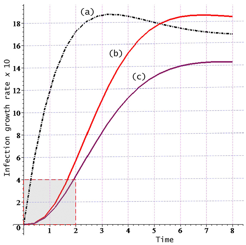
Infection growth rates for different epidemic threshold values: (a) Covid-19 initial spread rate in Turkey, (b and c) different forms of typical influenza.

Stages in epidemic cases

Spreading and recovery operations i a typical epidemic case follow a set of contiguous and interdependent stages, where each stage is modeled as a dynamic subsystem with adequately chosen state parameters. Each subsystem has some input and output parameters which change dynamically throughout the lifecycle of the epidemic case. In most cases, the subsystems are transient, and each subsystem feeds the input of its ancestor subsystem with data, while receiving data from its predecessor subsystem. Data exchanges between the subsystems take place through the individual state parameters of the associated subsystem. Each subsystem has its own population of elements, where the number of elements in a subsystem is denoted by a numerical value called “state.” For example, state $n$ means that the related subsystem contains $n$ elements, and state transition denotes the change in the number of elements in a subsystem. Table 1 contains the state space for all populations of the generic model. A typical state transitions diagram shown in Figure 2, illustrates the interaction between the model subsystems. Following each state transition, the individual population sizes and some parameter values are subject to change. These parameters denote state transition probabilities affected by factors such as immunity, contact rate, and quarantine and recovery some efficiency of the hospitalization unit. Figure 2 shows the chain of state transitions. An associated probability distribution function is denoted together with the respective block (compartment). Each of these distributions/equations describes the state transition dynamics of the related compartment.

Table 1.

Compartmental states associated rate parameters.

Parameter space for state changes
Flow rate	Description	Population size changed
$λ_{hs}$	Healthy to susceptible	Susceptible: $s (t)$
$λ_{sh}$	Susceptible to healthy	Healthy: $h (t)$
$λ_{si}$	Susceptible to infected	Infected: $i (t)$
$λ_{iq}$	Infected to quarantine	Quarantined: $q (t)$
$λ_{qr}$	Quarantined to recovery	Recovered: $r (t)$
$μ_{rh}$	Recovered to healthy	Healthy: $h (t)$

Figure 2.

A compartmental representation of the states of the recurrent model.

As can be noted, elements of the populations iterate from state to state depicting a recurrent characteristic, where the population sizes are precisely expressed by the following state equations, equation (8).

\begin{matrix} h (0, T] = h (t) + \sum_{t = 0}^{T} [λ_{sh} \times s (t) + μ_{rh} \times r (t) - λ_{hs} \times h (t)], \\ s (0, T] = s (t) + \sum_{t = 0}^{T} [λ_{hs} \times h (t) - λ_{sh} \times s (t) - λ_{si} \times s (t)], \\ i (0, T] = i (t) + \sum_{t = 0}^{T} [λ_{si} \times s (t) - λ_{iq} \times i (t)], \\ q (0, T] = q (t) + \sum_{t = 0}^{T} [λ_{iq} \times i (t) - λ_{qr} \times q (t)], \\ r (0, T] = r (t) + \sum_{t = 0}^{T} [λ_{qr} \times q (t) - μ_{rh} \times r (t)] . \end{matrix}

(8)

As also illustrated in Figure 2, some fractions of elements are flowed from population to population at different intensities, for example, from healthy to susceptible at rate $μ_{h_{s}}$ and from susceptible to infected at rate $λ_{si}$ .

State variables contain the time-dependent number of objects in a given epoch $(t, T]$ for the related state. For example, as depicted by equation (8), during the time slot $(0, T]$ , a proportion of the recovered population is moved to the healthy population, while some healthy objects remain susceptible. Likewise, a proportion of the susceptible population will become infected, some of the infected objects are quarantined, and a proportion of the quarantined objects recover. Consequently, at time $t + T_{x}$ , the number of objects in the respective population will be changed in a recursive manner.¹

Using notations from queuing theory, the stages (compartments) of the generic model will be described in the following sections. Arrivals of an object to a stage and operation completion (departure) from a stage are modeled as an M/M/1:(FCFS) queueing system. Based on this first-come first-served (FCFS) principle, each stage in the system encompasses a cascaded queueing system, where each stage serves a unique function. The overall behavior of the system is illustrated by the flow diagram shown in Figure 2, where each stage is a dynamic component of the recurrent operations. Initially, at least one host must be infected in the Susceptible population for further development of a disease. Often a stochastic growth of the susceptibility takes place as a branching process. Thereafter, an epidemic outbreak (exponentially distributed process) is initiated in the susceptible population. Arrivals to the infection stage and most other stages are modeled as a Poisson process denoted as $λ_{x_{y}}$ , meaning that the arrival is from stage $x$ to stage $y$ . The compartments of the recurrent model, shown in Figure 2, will be detailed in the following sub-sections.

A generic model

In order to facilitate the analysis in a broader scope, a generic model is necessary, which can elucidate the most encountered stages of epidemiology. In order to support this idea, the model presented here is built upon five types of populations: (i) healthy, (ii) susceptible, (iii) infected, (iv) quarantined, and (v) recovered. Furthermore, we have two major assumptions: (a) all individuals/nodes in a sample population are initially susceptible, (b) if a node gets infected then it becomes the source (transmitter) of a branching process for spreading the infection. At the next time slot, some of the hosts in the population are susceptible, and some are transmitter, which can cause infections. Initialization of the susceptible population with empirically obtained data is necessary in order to keep analysis within an acceptable dynamic range until the equilibrium state is achieved.

Unless otherwise specified, the process of infection through recovery is considered as an M/M/1 queueing system with a single server having Poisson arrival (infection case) and exponentially distributed recovery service time (recovery case). More specifically, the system is an FCFS Markovian queue with exponentially distributed interarrival and departure (or service) rates: arrivals and departures are independently and exponentially distributed with rates $λ$ $μ$ , respectively. Hence, the service utilization factor is $ρ =$ “arrival rate/service rate,” that is, $ρ = λ / μ$ .

Two distinct populations (biological and computer) may have different levels of susceptibility, where the susceptibility of an object depends on the protection level for computers and immunity level for living individuals. The immunity level for living individuals has several parameters such as age, locality (e.g. kindergarten, chicken poultry), mobility, vaccination, and so on.

Spread and extinction dynamics of a disease can be analyzed by two fundamental methods, time-dependent and limiting (or equilibrium) behavior analyses. Analysis of time-dependent behavior can help determine the number of patients (or hosts) under care by computing the probability that at time $t$ there are $n$ hosts in the system. System dynamics can be easily traced by the continuous Markov chain modeled as a birth–death process. A process is in state $n$ means that population (e.g. infected population) size is $n$ . Transition from state $n$ to state $n + 1$ is denoted as a birth, whereas a transition from state $n$ to $n - 1$ depicts a death. Both births and deaths occur only to the adjacent state (e.g. from $x$ to $x + 1$ or from $x$ to $x - 1$ ) with rates $λ$ and $μ$ , respectively. Birth and death rates are independent of time and of each other, and only dependent on the current state. The following definitions are used to describe the basic functions for the state transitions taking place in a given phase.

Definitions

$P_{0} (t) \equiv$ Probability of no state change during time $t$ ,

$P_{1} (t) \equiv$ Probability of a single state change during time $t$ ,

$λ Δ t \equiv$ Probability of an arrival (birth) with rate $λ$ in $Δ t$ ,

$μ Δ t \equiv$ Probability of a departure (death) with rate $μ$ in $Δ t$ ,

$1 - λ Δ t \equiv$ Probability of no arrival in $Δ t$ ,

$1 - μ Δ t \equiv$ Probability of no departure in $Δ t$ .

Healthy to susceptible

All starts with a susceptible object having contact with one or more transmitter objects. The susceptible objects can be infected and become an active transmitter after the latent period. Following this, an epidemic outbreak will occur. The outbreak is best modeled as a branching process, see Athreya and Ney⁵⁷ and Kalinkin⁵⁸ for a general review of branching processes. A branching process is a regenerative Markov process, where an individual in a population goes through a recursive regeneration process that proliferates in the next generation with a specific probability.

Let us assume a group of transmitter objects have contact with some susceptible objects, where the contacts and eventual infections are independent of each other. Here, the probability of a contact causing $k$ infections is denoted by $p_{k} (t)$ . Following the initial infection phase, $n - k$ nodes out of $n$ become susceptible, which will then initiate an epidemic outbreak as a branching process ( $ξ$ ). The branching process evolves as a pure birth (Poisson) process with the basic transition rates expressed as

ξ_{λ} = {\begin{matrix} p_{i, i} = - λ, \\ p_{i, i + 1} = λ, \\ p_{i, j} = 0, for j \neq (i, i + 1) . \end{matrix}

Besides these one-step transitions, transitions from $i$ to $j$ occurring in $n$ steps will approximate to a Bernoulli process performed $n$ times having the probability of success $λ$ given by

P {ξ = j | n} = {\begin{matrix} (\begin{matrix} n \\ j - 1 \end{matrix}) λ^{j - 1} (- λ)^{n - (j - i)} \\ 0, otherwise, for 0 \leq j - 1 \leq n \end{matrix}

(9)

The Poisson approximation of the above distribution is

P_{ξ} (j) ~ \frac{λ^{j}}{j!} e^{- λ}, λ = n p_{s} .

(10)

A small proportion of the susceptible population may be well-protected or may have sufficient level of immunity, and hence, will not become infected. Hence, the proportion of the susceptible hosts returning to the healthy population is depicted by $R_{s_{h}}$ , which depends on the current population sizes ( $R_{s_{i}}$ , $R_{ss}$ ) and rate parameters, susceptible–to–infected ( $λ_{si}$ ) and susceptible–to–susceptible ( $λ_{ss}$ ) given by

\frac{\partial R_{s_{h}}}{\partial t} = R_{s_{h}} - R_{s_{i}} (t) λ_{si} - R_{ss} (t) λ_{ss} .

(11)

Susceptible to infection

Assume that we have a population consisting of $N$ susceptible and $N - k$ homogeneously infected hosts each infecting some susceptible hosts independently of all the others. Each of the transmitters initially cause a small probability $p (t)$ of infection during time slice $t$ . Assuming a Poisson process with very large $N$ then the probability $p (t)$ of infection becomes very small (property of Poisson distribution contra Binomial), then the distribution of infection described by process $ξ (t)$ becomes accurately a Poisson distribution, especially when $N$ approaches to infinity. Thus, the probability of finding exactly $k$ infections will become

P [ξ (t) = k] = \frac{n^{k} t}{k!} e^{- nt}, k = 0, 1, 2, \dots,

(12)

However, if the population has a small number of individuals, in which each infection being considered as a “success” in a Bernoulli process. Then, $ξ (t)$ will hold the number of successful outputs in a series of $N$ Bernoulli trials performed in $t$ time units.

P [ξ (t) = k] = (\begin{matrix} N \\ k \end{matrix}) p (t)^{k} (1 - p)^{N - k}, k = 0, 1, 2, \dots,

(13)

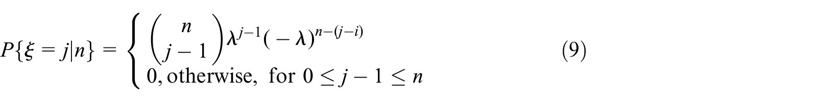
As can be noted, the infection phase consists of two sub–phases: first, some susceptible hosts, which are vulnerable (or unprotected), will be infected with a rate depending on the infection probability and density of the susceptible nodes. A second sub-phase consisting of a virus spread that starts through the currently infected nodes, as a branching process expressed by the following distribution,¹

P_{k} (t) = e^{- λ t} (1 - e^{- λ t})^{(k - 1)}; k \geq 1,

(14)

where $λ$ denotes the branching rate and $k$ is the current number of offspring generated from a single infection at time $t$ . Equation (14) is based on a single infectious node that initiates the branching of new infections. It should be reminded that, each infectious node causing a new infection in a small epoch $Δ t$ is a Markovian birth, that is, $λ Δ t + o (Δ t)$ .

Example

Assume we have a record of 180 infection cases a month. We need to determine (a) the probability of eight incidents per day, (b) the probability of at most five cases in a day

(a)There are $λ = 180 / 30 = 6$ cases per day on average, which is the rate of infection per day. Then,

P {x = 8} = \frac{λ^{x}}{x!} e^{- λ} = \frac{6^{8}}{8!} e^{- 8} = 0.103,

(b) $\begin{matrix} P {x \geq 4} = 1 - (P {x = 0} + \dots + P {x = 4}) \\ = 1 - (\frac{6^{0}}{0!} e^{- 6} + \dots + \frac{6^{4}}{4!} e^{- 6}) = 0.725 . \end{matrix}$

The results of a simulation with the Poisson distributed infection threshold and branching convoluted with Gamma distribution are plotted in Figure 3.

Figure 3.

Illustration of rates for the spread of infection evolving as a branching process.

As can be noted, recovery starts soon after the infection starts. This enforces a small diminish in branching rates modeled as Gamma function. Gamma distribution is tied with the immunity growth that enforces annihilation of the spread, with the degree of immunity. The curve in Figure 3(b) shows the branching rate changes with an insignificant incubation time, whereas 3(c) shows the effect of latent incubation times.

Infection to quarantine

Assume that, following an epidemic outbreak, we have a group of arrivals of patients with a Poisson rate $λ_{iq}$ . This process entails the discovery process, where a rapid diagnose is performed on each request in order to determine false positives. It is a fact that, the probability of no infection discovery during $t + Δ$ is

p_{0} (t + Δ t) = p_{0} (0, t) [1 - λ_{iq} Δ t],

a single discovery in the time interval $(t, t + Δ t)$ is

p_{1} (t, t + Δ t) = λ_{iq} Δ t,

the probability for more than one cases is expressed by

p_{n} (t + Δ t) = p_{n} (0, t) [1 - λ_{iq} Δ t] + p_{(n - 1)} (0, t) λ_{iq} Δ t .

The diagnose process proceeds as follows. It will be shown that $p_{0} (t) = e^{- λ_{iq} t}$ , and thus, the probability of $n$ arrivals during some time interval is proved by induction as:

P {I_{q} = n | λ_{iq}} = \frac{{(λ_{iq} t)}^{n}}{n!} e^{- λ_{iq} t} .

(16)

The infection–to–quarantine rate parameter, $λ_{iq}$ , denotes the mean arrival rate to the quarantine service.

Let us now determine the distribution of the transition time from infection to the quarantine stage, which we model as a memoryless process, where let the state $s_{0}$ be the state at time $t = t_{0}$ and $υ$ be the random time it takes the process to leave the state $s_{0}$ by going to some other state, then

φ (t) = P {υ > t} = e^{- λ_{iq} t}, t \geq 0,

(17)

where $λ_{iq}$ denotes the density of the departure from state $s_{0}$ . If $λ_{iq} = 0$ , the process will remain forever in $s_{0}$ , however, if $λ_{iq} > 0$ , the probability will be $λ_{iq} Δ t + o (Δ t)$ , denoting the probability of a change in the state during $Δ t$ . It follows from equation (17) that $P {υ > t}$ is some function of $t$ . If, assume, $φ (s) = P {υ > s}$ , then the process will be in the same state at time $t_{0} + s$ as at time $t_{0}$ , and hence its subsequent behavior will be similar to that of $s = 0$ . Especially,

φ (t) = P {υ > s + t | υ > s}

(18)

will obtain the probability of event $υ > s + t$ given that $υ > s$ . Then,

φ (t) φ (s) = P {υ > s + t | υ > s} P {υ > s} = P {υ > s + t},

(19)

and hence,

φ (s + t) = φ (t) φ (s) .

(20)

Then, the random variable $υ$ , called sojourn time in the current state, has the probability density given by

\begin{matrix} p_{υ} (t) = \frac{P [(υ > s + t) \cap (υ > s)]}{P (υ > s)} = \frac{P (υ > s + t)}{P (υ > s)} \\ = \frac{e^{- λ_{iq} (s + t)}}{e^{- λ_{iq} s}} = e^{- λ_{iq} t} = P {υ > t}, \end{matrix}

(21)

p_{υ} (t) = {\begin{matrix} λ_{iq} e^{- λ_{iq} t}, if t \geq 1, \\ 0, if t < 0 . \end{matrix}

Thus, the infection to quarantine time is exponentially distributed.

Quarantine to recovery

As shown in the previous sub-section, nodes in the infected population (or network) are inspected, where false positives are discovered in significantly short times. Regarding the computer viruses, users generally discover malfunctioning of computers at random when they turn on the computer. A simple birth–death process is appropriate for modeling the discrimination of real infection events and false positives, where a successful diagnose of an infection and a false positive can be obtained by

\begin{matrix} α_{k} = ϕ (m - k) + υ, \\ birth : p_{k, k + 1} = [ϕ (m - k)] \frac{1}{α_{k}}, \\ death : p_{k, k - j} = [ψ (\begin{matrix} k \\ j \end{matrix}) q^{j} {(1 - q)}^{k - j}] \frac{1}{α_{k}} . \end{matrix}

(22)

Here, $q$ is the probability that a detection is indeed a false detection (death), which is considered as a diagnostic process consuming negligible (zero) time. The population size is $m$ , $ϕ$ denotes the rate of the infection discovery, that is, rate of births in $t$ time units, and $ψ$ denotes the inspection rate.

For the stationary state, the probability of exactly $j$ nodes being detected as infected is then obtained by

P_{ξ} {ξ = j} = p_{j} = \frac{m!}{(m - j)!} {(\frac{ϕ}{ψ})}^{j} p_{0}, j = 0, 1, \dots, m,

(23)

where, $p_{0}$ is determined from the condition

\begin{matrix} \sum_{j = 0}^{m} p_{j} = p_{0} \sum_{j = 0}^{m} ρ^{j} = p_{0} \frac{1}{1 - ρ)} = 1, \\ p_{0} = 1 - ρ, ρ = ϕ ψ . \end{matrix}

The average number of nodes discovered as infected and awaiting for recovery is given by

E [I_{k}] = k - \frac{ϕ + ψ}{ϕ} (1 - p_{0}) = k - \frac{ϕ + ψ}{ϕ} (\frac{ϕ}{ψ}) .

(24)

Mortality rate

The probability $p_{j}$ from equation (23) incorporates the exponential infection rate $ϕ$ from the related Poisson distribution, where $ϕ = 1 - e^{- ϕ t}$ , then

n = E [ξ (t)] = m p_{j} (t) = m (1 - e^{- ϕ t})

as the average number of infected objects, whereas the number of lost objects is simply given by

\begin{matrix} \bar{n} = m - ξ (t) = E [m - ξ (t)] \\ = m - m p_{j} (t) = m e^{- ϕ t} . \end{matrix}

The reader is encouraged to determine the mortality in terms of $E [I_{k}]$ from equation (24).

Recovery to healthy

Total recovery (or hosting) time for individuals is denoted by an exponentially distributed random variable, $μ_{rh}$ , where each individual waits for at least $T$ random time slots and eventually requires more time unit denoted by $δ$ during the hosting period, then,

P {T \geq δ} = e^{- μ_{rh} δ}, t \geq 0,

(25)

will give the probability for determining the total time required for the overall hosting of a patient. Let the times between various hostings be denoted by a Poisson process, $H$ , with parameter $μ_{rh}$ denoting the rate of recovery of an individual. Thus, $H$ has the probability density function

f_{h} (t) = μ_{rh} e^{- μ_{rh} t} .

Hence, the mean time between recoveries is given by

E (H) = \frac{1}{μ_{rh}} .

The recovery process described by equation (25) can be simply modeled with two states, idle $s_{0}$ and busy $s_{1}$ , respectively. Assume a recovery facility is in an idle state at time $t_{0}$ , and due to the memoryless property of the Poisson arrivals, the probability $p_{0, 1} (Δ t)$ of the system going from state $s_{0}$ to state $s_{1}$ during $Δ t$ is just the probability as described earlier by $λ Δ t + o (Δ t)$ . As can be noted, the density of the transition from $s_{0}$ to $s_{1}$ is denoted by $λ$ . However, assume the system is in the busy state $s_{1}$ (processing an input request) at time $t$ , then the probability of a system moving from the busy state ( $s_{1}$ ) to the idle state ( $s_{0}$ ) is $p_{1, 0} (t)$ . Assuming the recovery service has been busy for $υ$ time units at time $t$ , then the probability for the idle state of the recovery unit is

p_{1, 0} (t) = 1 - P {T > υ + t | T > υ} = 1 - \frac{P {T > υ + t}}{P {T > υ}} .

(26)

Hence, plugging equation (25) into equation (26), we get the simplified equation for the transition probability from busy to idle state as

p_{1, 0} (t) = 1 - \frac{e^{- μ_{rh} (υ + t)}}{e^{- μ_{rh} υ}} = 1 - e^{- μ_{rh} υ} = μ_{rh} Δ t + o (Δ) t .

(27)

Obviously, we have a Markov process satisfying the following conditions

p_{0, 1} (t) = 1 - p_{0, 0} (t), p_{1, 0} (t) = 1 - p_{1, 1} (t) .

(28)

We have the facts

(\begin{matrix} λ_{0, 0} = - λ & λ_{0, 1} = λ \\ λ_{1, 0} = μ & λ_{1, 1} = - μ \end{matrix}),

(29)

and

p_{i, j} (0) = {\begin{matrix} 1, if j = i, \\ 0, if j \neq i \end{matrix}

(30)

to our disposal. Transition density from state $s_{i}$ is denoted by $λ_{i}$ and from state $s_{i}$ to state $s_{j}$ is denoted by $λ_{i, j}$ , respectively. As can be noted service times for recovery are exponentially distributed with parameter $μ_{rh}$ and requests arrive as Poisson distributed expressed as

\begin{matrix} p_{0, 1} (Δ t) = 1 - e^{- λ Δ t} = λ Δ t + o (Δ t), \\ p_{1, 0} (Δ t) = 1 - e^{- μ Δ t} = μ Δ t + o (Δ t) . \end{matrix}

(31)

Recovery facility with single serviceman

We need to determine the limiting solutions so that we can easily determine the mean requests awaiting for the recovery at any time. Suppose we have a service facility with a single repairman (server) handling at most $m$ identical incoming requests. We assume also the incoming requests are Poisson distributed with mean arrival rate $λ$ , where each request has probability $λ Δ t + o (Δ t)$ and their arrivals are independent of each other. Thus, the recovery process is modeled as a Markov process, where recovering a request is exponentially distributed with parameter $μ$ . To find the limiting probabilities for the recovery process we consider the following relations associated to transition densities both for the arrivals and departures of the requests.

\begin{matrix} lim_{t \to 0} \frac{p_{j, j + 1} (t)}{t} = (m - j) λ, for j = 0, 1, \dots, m, \\ lim_{t \to 0} \frac{p_{j, j - 1} (t)}{t} = {\begin{matrix} μ, for j = 1, 2, \dots, m, \\ 0, for j = 0, \end{matrix} \\ lim_{t \to 0} \frac{1 - p_{jj} (t)}{t} = {\begin{matrix} (m - j) λ + μ, for j = 1, 2, \dots, m, \\ m λ, for j = 0 . \end{matrix} \end{matrix}

We can obtain the limiting probabilities by solving the following system of equations

\begin{matrix} m λ p_{0} = μ p_{1}, \\ μ p_{m} = λ p_{m - 1}, for j = m, \\ [(k) λ + μ] p_{j} = (k + 1) λ p_{j - 1} + μ p_{j + 1}, \\ for k = m - j, j = 1, \dots, m - 1 . \end{matrix}

(32)

Hence, solving this system of equations, the limiting probability of exactly $j$ requests present in the system is obtained by

p_{j} = \frac{m!}{(m - j)!} {(\frac{λ}{μ})}^{j} p_{0}, j = 1, 2 \dots, m .

(33)

Thus, based on the condition $\sum_{j = 0}^{m} p_{j} = 1$ ,

p_{0} = \frac{1}{\sum_{j = 0}^{m} [\frac{m!}{(m - j)!} {(\frac{λ}{μ})}^{j}]} .

We can now determine the limiting probability of exactly $j$ requests being recovered by solving the following system of equations.

\begin{matrix} m λ p_{0} = μ p_{1}, \\ m μ p_{m} = λ p_{m - 1}, for j = m, \\ [(k) λ + j μ] p_{j} = (k + 1) λ p_{j - 1} + (j + 1) μ p_{j + 1}, \\ for k = m - j, j = 1, 2 \dots, m - 1 . \end{matrix}

(34)

Thus, the limiting probability $p_{j}$ leading to exactly $j$ recoveries out of $m$ requests is

p_{j} = (\begin{matrix} m \\ j \end{matrix}) {(\frac{μ}{λ + μ})}^{m - j} {(\frac{λ}{λ + μ})}^{j}, for j = 0, 1, \dots, m .

(35)

It should be noted that these analyses assume $m$ identical requests each handled independently of the others.

Example: Resource utilization

Let us assume that a healthcare center randomly receives an average of 128 patients each 24 h. The center spends on average 8 min on each patient, where each individual is treated one at a time. Based on this information, we can determine a set of useful results regarding (a) proportion of the time the center is busy, (b) system utilization, and (c) mean service rate, (d) probability of the number of patients at the center, (f) idle time of the system.

Assume that the care center is modeled as an $M / M / 1$ queue system with Poisson arrivals of patients and exponentially distributed service (diagnose + care) times. First, average arrival rate of patients per hour is

λ = 128 / 24 = 5.333 / h .

Average service rate per hour is

μ = (8 / 60)^{- 1} = (2 / 15)^{- 1} = 7.500 / h .

System utilization (proportion of busy time) is

ρ = λ / μ = 5.333 / 7.500 = 0.7111 / h .

Probability of having the system idle (i.e. exactly 0 patient under care) is

p_{0} = (1 - ρ) = (1 - 0.7111) = 0.289 .

Probability of having exactly one patient under treatment is

p_{1} = (1 - ρ) ρ^{1} = (1 - 0.7111) 0.7111 = 0.205 .

Probability of having more than one patient under treatment is

\begin{matrix} p_{(n > 1)} = 1 - p_{(n \leq 1)} = (1 - p_{0}) ρ = 1 - (p_{0} + p_{1}) \\ = 1 - (0.289 + 0.205) = 0.506 . \end{matrix}

(36)

Recovery facility with random service rates

Throughput of a service facility is one of the dominating factors for jobs with large and randomly fluctuating backlogs. It is also important for us to introduce this case here. Generally, higher workload may lead to a situation of “panicking” server resulting in diminished throughput, whereas lower workload may divert system to a “lazy” server, also resulting in diminished throughput. It is often suitable to assume constant mean service rates for systems involving automated or machinated services. However, in reality, queueing systems involving human servers cannot always have constant rates. For example, increased incoming requests (e.g. patient flow into an emergency unit in a hospital) may result in increased pressure on the doctors/nurses undertaking the service. This will, in turn, result in increased effort and higher service rate, or even cause a worsened situation due to the higher pressure. On the other hand, when the backlog (queue length) is small, then the service rate will decrease, due to the “lazy” server syndrome. More on the related issues can be found in Gross et al.,⁵⁹ Stewart,⁶⁰ and Asmussen.⁶¹ One can also refer to Schwarz⁶² for more detailed analysis of time-dependent queueing systems.

Suppose we have a system with state space $ξ [0, 1, 2, \dots, n]$ behaving as a continuous-time birth–death process having birth rates $λ_{j}$ and death rates $μ_{j}$ , where $j$ is the current number of requests present in the system. The transition probabilities

p_{i, j} (t) = P {ξ (t) = j | ξ (0) = i}, (i, j) \in ξ [0, 1, 2, \dots]

need to satisfy the forward Kolmogorov equations

\begin{matrix} \frac{\partial p_{i, 0} (t)}{dt} = - λ_{0} p_{i, 0} (t) + μ_{1} p_{i, 1} (t) \\ \frac{\partial p_{i, j} (t)}{dt} = λ_{j - 1} p_{i, j - 1} (t) - (λ_{j} + μ_{j}) p_{i, j} (t) + μ_{j + 1} p_{i, j + 1} (t) . \end{matrix}

We then have for a system having stationary characteristics

lim_{t \to \infty} p_{i, n} (t) = p_{n} = P {ξ = n} .

Hence, we have the limiting distribution $\forall p_{i}, i = 0, 1, 2 \dots$ , and as detailed in Appendix, we have

p_{n} = p_{0} Π_{i = 1}^{n} \frac{λ_{i - 1}}{μ_{i}},

where

p_{0} = {[1 + \sum_{k = 1}^{\infty} Π_{i = 1}^{k} \frac{λ_{i - 1}}{μ_{i}}]}^{- 1} .

On the basis of the non-catastrophic constrain we also have the following relation.

(\frac{p_{i}}{p_{i - 1}}) = (\frac{λ_{i - 1}}{μ_{i}}), p_{i} = (\frac{λ_{i - 1}}{μ_{i}}) p_{i - 1}, for i = 0, 1, 2, \dots

Again, assuming Poisson arrivals with $λ$ and exponential service times denoted by $μ_{n}$ . A new parameter ( $R$ ) is now needed to represent the degree to which the server is affected due to the large backlog, where the queue length is $n$ . Therefore, the mean service rate for $n$ requests will be

μ_{n} = n^{R} μ_{1}, R = 0, \dots, 1, n = 1, 2, \dots,

(37)

where, $R$ represents a random coefficient denoting the stress factor and $μ_{1}$ stands for the expected service time when there is only one request in the queue. Hence, the overall throughput ratio of a queue with $n$ requests will be

\sum_{n}^{R} = \frac{1}{{(n!)}^{R}} {(\frac{λ}{μ_{1}})}^{n}, n = 1, 2, \dots, .

(38)

The negative effect of large backlogs leads to decrease in the service rate. This can be due to the annoyance of individuals waiting longer than expected, or diverting the requests to other facilities, if available. Such cases will typically lead to decreased arrivals, where a random coefficient, $D$ , affects the growth rate of the input queue given in

λ_{n}^{D} = λ_{0} (n + 1)^{- D} n = 1, 2, \dots, .

(39)

This random fluctuating with large backlogs is illustrated in Figure 4, which depicts the result of a simulation with random mean service rates satisfying the relation of $ρ \leq \frac{λ}{μ}$ .

Figure 4.

The effect of fluctuating arrivals causing increased service times: (a) input queue, (b) increased service time with random fluctuations affected by large backlog, and (c) decreased steady-state departure rime.

Experiments and simulations

One may need to experiment a chosen model with different cases and scenarios in order to validate it, that is, to determine whether it can produce expected results. Experiments should be better combined with simulations so that they can be numerically verified based on various scenarios. It is usually trivial to simulate computer epidemics due to more concrete definition and fewer number of the system parameters compared to that of human epidemics. In fact, some human viral infections behave similarly to that of computer infections, and can be easily adapted to computer simulations. For example, some human/animal viruses attack certain cells and proliferate within the attacked victims in the same way as a computer worm spreads itself. Therefore, we can modify some validated computer virus scenarios to match the biological viral infection cases and scenarios. The scenarios can then be experimented with in a network laboratory to observe the spread and control of infections, and the results are then justified with computer simulations. The simulation can then be expanded to evaluate a variety of biological epidemics, if desired. For example, CMV: cytomegalovirus, HPV: Human Papilloma, HTLV: Human T-Lymphotropic, rubella, influenza, Herpes 1 and Herpes 2 are the family of human viruses, where their propagation patterns can be justified by computer simulations, if appropriate models with sufficient amount of data are available.

In order to emphasize the diversity (or similarity) between the human and computer epidemics, a simulation of two related cases was conducted, where both processes have Poisson input, but their recovery processes evolved differently. It was shown that the human recovery process involves the Gamma distributed recovery process. This result is realistic, due to the automatically grown immunity found in human intelligence.⁶³ Figure 5 illustrates results of the simulations with constant infection rate of $λ = 10$ distributed by a Poisson Distribution. A large susceptible population size with minimal probability of infection can be modeled by a Poisson process, whereas higher probability and smaller population size will approximate to Binomial distribution.

Figure 5.

Simulation results depicting the infection and recovery characteristics of human and computer cases each having 1000 hosts.

The recovery is exponentially convolved with Gamma distribution. Gamma convolution increases the accuracy of recovery due to increased immunity of the infected objects while undergoing recovery. Based on a simulation, the changes in a population of 1000 nodes are shown in Figure 5.

Treatment evaluation

The efficiency of a healing method (or protection) can be evaluated to determine whether it is reliable during the course of its application. The model given here is straightforward, where the probability of a single failure and success of a treatment develops as a simple birth–death Markov chain. It is assumed that healing fails with rate $λ$ and succeeds with rate $μ$ , where both rates are constant. Constant rate means that a given event occurs with a certain frequency during a specified time unit. For example, drug A cures 65% of patients of age 60–65 after 14 dosages. Thus, we can define two mutually exclusive states (success and fail) for the healing method at hand. Based on the definitions for the state transitions defined earlier, we can obtain the probability for the success or failure of a treatment. Let us first assume the following definitions for two time variables, $t$ and $Δ t$ :

$P_{s} (t)$ : probability of success,

$P_{f} (t)$ : probability of failure,

$λ Δ t$ : probability of failure in $Δ t$ , that is, probability of transition from state success to failure in $Δ t$ .

$μ Δ t$ : probability of success in $Δ t$ , that is, probability of transition from state failure to success in $Δ t$ ,

$1 - λ Δ t$ : probability of not failing in $Δ t$ ,

$1 - λ Δ t$ : probability of not succeeding in $Δ t$ .

Hence, we can deduce the following set of equations to describe the probability of state transitions occurring during $t + Δ t$ .

\begin{matrix} P_{s} (t + Δ t) = P_{s} (t) [1 - λ Δ t] + P_{f} (t) μ Δ t \\ P_{f} (t + Δ t) = P_{f} (t) [1 - μ Δ t] + P_{s} (t) λ Δ t \end{matrix}

(40)

These linear equations deal with a single item, which can be in any of two mutually exclusive Markovian states at a time, either failure (birth) or success (death). Hence, failure of a treatment is depicted by a birth process, whereas a success is depicted by a death process. Prior to solving these equations we rewrite them in the form of differential equations as.

\begin{matrix} \frac{\partial P_{s} (t)}{dt} = - λ P_{s} (t) + μ P_{f} (t) \\ \frac{\partial P_{f} (t)}{dt} = - μ P_{f} (t) + λ P_{s} (t) . \end{matrix}

Solutions of these equations can be obtained by applying various methods, for example, Laplace transform, recursive numerical method, Langranges, and transition matrix. Thus, by setting $P_{s} (0) = 1$ at $t = 0$ and applying Laplace transform, we can obtain a general solution to express the probability of failure $P_{f} (t)$ and success $P_{s} (t)$ , respectively. Setting $ψ = λ + μ$ , we have

Success : P_{s} (t) = \frac{μ}{ψ} + \frac{λ}{ψ} e^{- ψ t}

Failure : P_{f} (t) = 1 - P_{s} (t) = \frac{λ}{ψ} - \frac{λ}{ψ} e^{- ψ t} .

(41)

Predator–prey cases

In computer networks, we can have predator software that can fight against malware in real-time. Internet pop-up and Trojan blockers should work in this way. However, most anti-virus programs are usually configured to run periodically or manually, which then cannot be considered as dynamic predators. Because computer malware (worm, virus) are frequently and randomly deployed in different forms, discovering them in real-time becomes extremely difficult. The predator-prey model has a periodic behavior because the effect of hunting and surviving changes relative to the respective population growth rates. Lotka-Volterra predator-prey model has been frequently referred to for describing the relation between a predator and its prey, where the predator consumes the prey to survive. Increasing the level of consumption leads to higher starvation rates, especially if a certain prey is the only source of survival for many different predator types.

Let us simulate a scenario dealing with computer viruses in order to observe the power of predators behaving as a benign computer virus. The following differential equation, equation (42), models an anti-virus as the prey, where a computer virus plays the role of the predator, which is also programmed to destroy (stop) as many as anti-viruses as possible. Population parameters are $< a, A >$ and $< b, B >$ for the predators and preys, respectively. Each time the predator destroys an anti-virus (prey), the predator population grows following the Poisson distribution with the density parameter $λ$ . However, the prey has an immunity growth feature against the predator attacks, see Attack-obstacle model in Kondakci.⁶³ Preys gain intelligence that proliferates them with a certain rate each time they survive an attack. Hence, the immunity growth of the prey follows the Gamma distribution with $α$ and $β$ as the shape and scale parameters, respectively.

\begin{matrix} \frac{\partial a}{dt} = a [1 - \frac{b}{B}] [\frac{λ^{x}}{x!} e^{- λ}] \\ \frac{\partial b}{dt} = - b [1 - \frac{a}{A}] [\frac{x^{α - 1}}{β^{α} Γ (α)} e^{- x / β}] . \end{matrix}

(42)

Figure 6 illustrates the simulation results obtained from the model given in equation (42).

Figure 6.

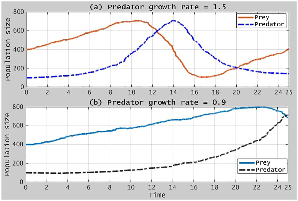
Illustration of the predator-prey relation.

As shown in the figure, the rate changes have also random characteristics, because virus attacks are random, that is, by nature hunting and surviving occur in a random fashion. Ideally, the system can come to an equilibrium point, where the effect of infection rate will be governed by the prey population as shown in Figure 7.

Figure 7.

Illustration of the steady–state in the predator-prey extinction state.

Discussion

Designing accurate models can significantly mitigate the number of cases and mortalities. Models developed for computer epidemics cannot be directly applied to human epidemics, and vice versa. Computer epidemics differ from human epidemics in some aspects. For example, incubation (latent) time for computer viruses can be extremely short, and even in some cases unpredictably long. On the other hand, latent time depends generally on the type of virus for human epidemics, and depends minimally on the individual’s immunity.

We generally consider analysis of epidemics under two different numerical approaches, deterministic, and stochastic. Deterministic models can be simple to apply, in which the limiting distributions can be obtained more easily with fewer parameters. On the other hand, stochastic models have more sophisticated stages of analysis, which allow fine-graining of parameters for more precise results. This feature leads naturally to more time needed for analysis in order to achieve the equilibrium state, hence manual computation of results is infeasible for large data set, for example, more than 10 observations. Another limitation is the level of learning threshold, which may hinder its application in some environments.

Designing of an extended stochastic model is planned as a future work, in which the extension will deal with new births (connections coming from external networks), mortality, and cases of pandemics dealing with infectious agents exported to external networks.

Conclusions

It is important to build models reflecting realistic characteristics of a given case, including effective resource planning, estimation of future risks, and reliable measures for mitigation. This paper presented a generic model for analyzing the epidemic stages and their interaction with each other. In most cases, epidemiology is a stochastic process involving several stages of evolution. Therefore, applying queueing theory enhanced with stochastic analysis can give a better overview over the dynamics of epidemic cases. Although the correctness of other models (e.g. deterministic, diffusion, differential analysis) is undeniable, features of stochastic queue models can guide us to simpler and more structured solutions that can be realized using recursive computer algorithms and other numerical approaches. This paper has modeled all stages of an epidemic case, where each stage has been formulated thoroughly within a stochastic context, so that the approach can serve as a guide for building models applicable to different environments with stochastic behavior.

The approaches given here are applicable to both human and computer epidemics. Test and verification of models used for human epidemics can be validated by an associated computer model, where computes can be used as test objects representing the individuals of a human population. By this manner, we can acquire some key parameters that can be precisely used for the human model. For example, parameters such as immunity, incubation time, and infection rate can be adjusted to match the characteristics of a given virus attacking humans, and then run simulation with computers to obtain results reflecting the human epidemics caused by that virus. In order to increase the accuracy of a model we can set up various infection sceneries and configure a wide range of parameters and network sizes/types in a computer simulation. Hence, we can precisely obtain the characteristics of a given type of viral outbreak in a human population by fine-adjusting of the variables used for the simulation with computers as victims.

Footnotes

Appendix

Appendix B: Data sampling and rate estimation

Assuming a Poisson process with a collection of random observations that are independent and identically distributed, where the random variables all are mutually independent and have same probability distribution. If we want to determine an estimator for the rate parameter $λ$ , then we need to collect sufficiently large amount of observation data at different times slots, call the collection as $Ω = {X_{1}, \dots, X_{n}}$ ; all sampled from a Poisson( $λ$ )-distribution. A maximum likelihood estimator for $λ$ can then be determined by computing the joint density probability as a function of the unknown parameter $λ$ and maximize it over all possible values of $λ$ as

P {λ | X_{i}, \dots, X_{n}} = Π_{i = 1}^{n} \frac{λ^{X_{i}}}{X_{i}!} e^{- λ} .

In order to facilitate the computation of the estimator, the corresponding log-likelihood function of the joint density function followed by a derivation can be applied to find an estimate of the unknown parameter $λ$ . It is already known that the logarithm of a product is equal to sum of logarithms of the members of the product. Thus, the likelihood equation

(61)

\begin{matrix} ℓ {λ | X_{i}, \dots, X_{n}} = \sum_{i = 1}^{n} \log (\frac{λ^{X_{i}}}{X_{i}!} e^{- λ}) \\ = \sum_{i = 1}^{n} [(X_{i} \log λ - λ) - \log (X_{i}!)], \end{matrix}

and taking the derivative of the likelihood equation, equation (60), leads to the maximum likelihood estimator for $λ$ as

E [λ] = \frac{1}{n} \sum_{i = 1}^{n} X_{i} .

Acknowledgements

We would like to express our deepest appreciation to reviewers of this paper for their constructive comments, and Simon Edward Mumford for his excellent contribution in proof–reading of the paper.

Declaration of conflicting interests

The author(s) declared no potential conflicts of interest with respect to the research, authorship, and/or publication of this article.

Funding

The author(s) received no financial support for the research, authorship, and/or publication of this article.

ORCID iD

Suleyman Kondakci

Author biographies

Suleyman Kondakci received the EE Engineering degree from the University of Gazi, Turkey, BS, MS, and PhD degrees from the University of Oslo, Norway. He is a Professor in Computer Sciences. His research area and publications are mostly focused on biomedical engineering, stochastic modeling, epidemiology, ubiquitous computing, and security of critical systems.

Dilek Doruk Kondakci received the BS degree from Ege University, M.S. from Afyon Kocatepe University in Nursing, and PhD in geriatrics from Ege University. She has recently been involved in a number of EU projects in Elderly Health. Her current research projects and university teaching include public health, emergency, and geriatrics.

References

Kondakci

Dincer

. Internet epidemiology: healthy, susceptible, infected, quarantined, and recovered. Secur Commun Netw 2011; 4(2): 216–238.

Bhattacharya

Paul

Choudhury

. Different types of epidemic models and their characteristic behaviour by using matlab. J Interdiscip Math 2015; 18(5): 569–592.

Taha

. Operations research: an introduction. 10th ed. London, UK: Pearson, 2016.

Medhi

. Stochastic models in queueing theory. 2nd ed. Cambridge, Massachusetts, USA: Academic Press, 2003.

Cui

. Markov repairable systems with history-dependent up and down states. Stoch Model 2007; 23(4): 665–681.

Jiang

, et al. Clinical findings in a group of patients infected with the 2019 novel coronavirus (sars-cov-2) outside of Wuhan, China: retrospective case series. BMJ 2020; 368: m606.

Chen

. Pathogenicity and transmissibility of 2019-nCoV–a quick overview and comparison with other emerging viruses. Microbes Infect 2020; 22(2): 69–71.

Huang

Wang

, et al. Clinical features of patients infected with 2019 novel coronavirus in Wuhan, China. Lancet 2020; 395(10223): 497–506.

Amador

Artalejo

. Modeling computer virus with the BSDE approach. Comput Netw 2013; 57(1): 302–316.

10.

Amador

Artalejo

. Stochastic modeling of computer virus spreading with warning signals. J Franklin Inst 2013; 350(5): 1112–1138.

11.

Yang

Wang

Yao

. An immunization strategy for social network worms based on network vertex influence. China Commun 2015; 12(7): 154–166.

12.

Sellke

Shroff

Bagchi

. Modeling and automated containment of worms. IEEE Trans Dependable Secure Comput 2008; 5(2): 71–86.

13.

Kondakci

. Epidemic state analysis of computers under malware attacks. Simul Model Pract Theory 2008; 16(5): 571–584.

14.

Rohloff

Başar

. Deterministic and stochastic models for the detection of random constant scanning worms. ACM Trans Model Comput Simul 2008; 18(2): 1–24.

15.

Ortega

Alonso

Ortega

. Stochastic comparisons of mixtures of parametric families in stochastic epidemics. Math Biosci 2013; 243(1): 18–27.

16.

Britton

. Stochastic epidemic models: a survey. Math Biosci 2010; 225(1): 24–35.

17.

del Rey

. Mathematical modeling of the propagation of malware: a review. Secur Commun Netw 2015; 8(15): 2561–2579.

18.

Artalejo

Lopez-Herrero

. Stochastic epidemic models: New behavioral indicators of the disease spreading. Appl Math Modell 2014; 38(17): 4371–4387.

19.

Batista

Martín del Rey

Quintero-Bonilla

, et al. A SEIR model for computer virus spreading based on cellular automata. In: Proceeding of the International joint conference SOCO’17-CISIS’17-ICEUTE’17 (eds H

Pérez García

Alfonso-Cendón

Sánchez González

, et al.), León, Spain, 6–8 September 2017, pp.641–650. Cham: Springer International Publishing.

20.

Kenah

Robins

. Network-based analysis of stochastic sir epidemic models with random and proportionate mixing. J Theor Biol 2007; 249(4): 706–722.

21.

Nowzari

Preciado

Pappas

. Analysis and control of epidemics: a survey of spreading processes on complex networks. IEEE Control Syst 2016; 36(1): 26–46.

22.

Mukhopadhyay

Bhattacharyya

. Existence of epidemic waves in a disease transmission model with two-habitat population. Int J Syst Sci 2007; 38(9): 699–707.

23.

Hethcote

. The mathematics of infectious disease. SIAM Rev 2000; 42(4): 599–653.

24.

Paul

Mishra

. Worm propagation with differential infectivity under quarantine control strategy. Int J Secur Appl 2016; 10(8): 201–214.

25.

Ren

Liu

. Modeling the dynamics of a network-based model of virus attacks on targeted resources. Commun Nonlinear Sci Numer Simul 2016; 31(1–3): 1–10.

26.

Kudo

Kimura

Inoue

, et al. Stochastic modeling of self-evolving botnets with vulnerability discovery. Comput Commun 2018; 124: 101–110.

27.

Wang

Wen

Xiang

, et al. Modeling the propagation of worms in networks: a survey. IEEE Commun Surv Tutorials 2014; 16: 942–960.

28.

Cabrera

Calix

. On the anatomy of the dynamic behavior of polymorphic viruses. In: 2016 international conference on collaboration technologies and systems (CTS), Orlando, FL, USA, 31 October–4 November 2016, pp.424–429. New York: IEEE.

29.

Wong

Bielski

McCune

, et al. A study of mass–mailing worms. In: WORM ’04: Proceedings of the 2004 ACM workshop on rapid malcode, pp.1–10. New York: ACM Press.

30.

Fachkha

Debbabi

. Darknet as a source of cyber intelligence: survey, taxonomy, and characterization. IEEE Commun Surv Tutorials 2016; 18(2): 1197–1227.

31.

Anderson

Britton

. Stochastic epidemic models and their statistical analysis. New York, NY: Lecture Notes in Statistics Springer, 2000.

32.

Daley

Gani

. Epidemic modeling, an introduction. Cambridge: Cambridge University Press, 1999.

33.

Brauer

Castillo-Chavez

. Mathematical models in population biology and epidemiology. Berlin: Springer, 2001.

34.

Diekmann

Heesterbeek

. Mathematical epidemiology of infectious disease. Wiley Series in Mathematical and Computational Biology. Chichester: Wiley, 2000.

35.

Nah

Nakata

Rst

. Malaria dynamics with long incubation period in hosts. Comput Math Appl 2014; 68(9): 915–930.

36.

Lou

Zhao

. A reaction–diffusion malaria model with incubation period in the vector population. J Math Biol 2011; 62(4): 543–568.

37.

Pastor-Satorras

Vespignani

. Epidemics and immunization in scale-free networks. Wiley-VCH Verlag GmbH & Co. Weinheim, Germany: KGaA, 2004.

38.

Small

Walker

, et al. Epidemic dynamics on scale-free networks with piecewise linear infectivity and immunization. Phys Rev E 2008; 77: 036113.

39.

Sharif

Riley

Lee

. Comparative study between analytical models and packet-level worm simulations. In: PADS ’05: Proceedings of the 19th workshop on principles of advanced and distributed simulation. Washington, DC: IEEE Computer Society, pp. 88–98.

40.

Moore

Shannon

claffy

. Code-red: a case study on the spread and victims of an internet worm. In: IMW ’02: Proceedings of the 2nd ACM SIGCOMM workshop on internet measurment, pp.273–284. New York, NY: ACM Press.

41.

Moore

Paxson

Savage

, et al. Inside the slammer worm. IEEE Secur Priv 2003; 1(4): 33–39.

42.

Newman

. Power laws, Pareto distributions and Zipf’s law. Contemp Phys 2006; 46(5): 323–351.

43.

Clauset

Shalizi

Newman

. Power-law distributions in empirical data. SIAM Rev 2009; 51(4): 661–703.

44.

Barabási

. Scale-free networks: a decade and beyond. Science 2009; 325(5939): 412–413.

45.

Dietz

. The estimation of the basic reproduction number for infectious diseases. Stat Methods Med Res 1993; 2(1): 23–41.

46.

Driessche

Watmough

. Reproduction numbers and sub-threshold endemic equilibria for compartmental models of disease transmission. Math Biosci 2002; 180(1): 29–48.

47.

Zhao

Lin

Ran

, et al. Preliminary estimation of the basic reproduction number of novel coronavirus (2019-nCoV) in China, from 2019 to 2020: a data-driven analysis in the early phase of the outbreak. Int J Infect Dis 2020; 92: 214–217.

48.

Diekmann

Heesterbeek

JAP

Roberts

. The construction of next-generation matrices for compartmental epidemic models. J R Soc Interface 2010; 7(47): 873–885.

49.

Driessche

. Reproduction numbers of infectious disease models. Infect Dis Model 2017; 2(3): 288–303.

50.

Massad

Coutinho

FAB

Burattini

, et al. Estimation of R0 from the initial phase of an outbreak of a vector-borne infection. Trop Med Int Health 2010; 15(1): 120–126.

51.

Heffernan

Smith

Wahl

. Perspectives on the basic reproductive ratio. J R Soc Interface 2005; 2(4): 281–293.

52.

Yang

. The basic reproduction number obtained from jacobian and next generation matrices - a case study of dengue transmission modelling. Biosystems 2014; 126: 52–75.

53.

Hartemink

Randolph

Davis

, et al. The basic reproduction number for complex disease systems: defining R0 for tick-borne infections. Am Nat 2008; 171(6): 743–754.

54.

Nishiura

Chowell

Safan

, et al. Pros and cons of estimating the reproduction number from early epidemic growth rate of influenza A (H1N1) 2009. Theor Biol Med Modell 2010; 7(1): 1.

55.

Colizza

Barrat

Barthelemy

, et al. Modeling the worldwide spread of pandemic influenza: baseline case and containment interventions. PLoS Med 2007; 4(1): 1–16.

56.

Kondakci

. A concise cost analysis of internet malware. Comput Secur 2009; 28(7): 648–659.

57.

Athreya

Ney

. Branching processes, 1st ed. Springer-Verlag Berlin Heidelberg, 1972. https://doi.org/10.1007/978-3-642-65371-1

58.

Kalinkin

. Final probabilities for a branching process with interaction of particles and an epidemic process. Theory Probab Appl 1999; 43(4): 633–640.

59.

Gross

Shortle

Thompson

, et al. Fundamentals of queueing theory. 4th ed. Hoboken, NJ, USA: John Wiley & Sons, Inc., 2013.

60.

Stewart

. Probability, Markov chains, queues, and simulation. 1st ed. Princeton, NJ: Princeton University Press, 2009.

61.

Asmussen

. Applied probability and queues. 2nd ed. Springer Science+Business Media. New York, NY: Springer-Verlag, 2003.

62.

Schwarz

Selinka

Stolletz

. Performance analysis of time-dependent queueing systems: survey and classification. Omega 2016; 63: 170–189.

63.

Kondakci

. Analysis of information security reliability: a tutorial. Reliab Eng Syst Saf 2015; 133(0): 275–299.

64.

Nadarajah

. Probabilities for queueing systems with embedded markov chains. Stoch Anal Appl 2008; 26(3): 526–536.

Building epidemic models for living populations and computer networks

Abstract

Keywords

Introduction

Motivations and related work

Population structures

Centralized networks

Scale-free networks

Growth and extinction dynamics

Basic reproduction number

Epidemic threshold

Stages in epidemic cases

A generic model

Definitions

Healthy to susceptible

Susceptible to infection

Example

Infection to quarantine

Quarantine to recovery

Mortality rate

Recovery to healthy

Recovery facility with single serviceman

Example: Resource utilization

Recovery facility with random service rates

Experiments and simulations

Treatment evaluation

Predator–prey cases

Discussion

Conclusions

Footnotes

Appendix

Appendix B: Data sampling and rate estimation

Acknowledgements

Declaration of conflicting interests

Funding

ORCID iD

Author biographies

References