Sage Journals: Discover world-class research

Abstract

Extreme haze was often observed at many locations in Beijing–Tianjin–Hebei region within several hours when they occurred, which is referred to as extreme co-movements and extreme dependence in statistics. This article applies tail quotient correlation coefficient to explore the temporal and spatial extreme dependence patterns of haze in this region. Hourly PM2.5 station-level data during 2014–2018 are used, and the results show that the tail quotient correlation coefficient between stations increases with month. Specifically, the simultaneous extreme dependence was strong in the fourth season, while the haze was severe. In the first season, while the haze was also severe, the extreme hazes only show strong co-movements with a time difference. These observations lead to the study of two special scenarios, that is, the concurrence/extreme dependence of the worst extreme haze and its lag effects. City clusters suffering simultaneous extreme haze or with certain time difference as well as the most frequently co-movement cities are identified. The extreme co-movements of these cities and the reasons for their occurrences have strong implications for improving the PM2.5 joint prevention and control in the Beijing–Tianjin–Hebei region. The importance of lag effects is also reflected in the precedence order of the extreme haze’s appearance. It is especially useful when setting the mechanism of the early warning system which can be triggered by the first appearance of extreme haze. The precedence orders also avail in investigating the transmission path of the haze, based on which more precise meteorological models can be made to benefit the haze forecasting of the region.

Keywords

Climate extremes extreme dependence extreme value analysis particulate matters

Introduction

As a type of severe air pollution, haze is the consequence of both human beings’ action and climatic conditions. Los Angeles, Donora, London, and so on have been suffered from heavy haze in history.^1–3 Recently, haze problems in Italy, India, Pakistan, and China have also drawn worldwide attention.^4–9 Extensive research works from biochemistry and biomedicine areas have demonstrated that haze may bring harm to human’s health,¹⁰ including increasing the risk of adult mortality, preterm birth, and causing ocular surface diseases, Alzheimer’s disease, and so on.^8,11–13

Haze may result in welfare loss and a serial of social problems as well. Taking China as an example, haze may impact China’s agricultural production and decrease the satisfaction of international tourists, lead to an outflow of the labor force, and even enhance the risk of mood driving.^14–17 New protection techniques from PM2.5 have arisen^18,19 while PM2.5 emission, source apportionment,^20–23 and the impact of meteorological factors have also been studied.^24–26 Pollution reduction measures and control strategy have also been proposed.^27,28 PM2.5 monitoring and the assessment of satellite or ground observations have been widely focused as well.^29–31

Researchers have studied the variation, nonlinearity, and spatial correlation of PM2.5 concentration or its adjusted value in China.^32–37 For example, the long-term variation trend in satellite-derived PM2.5 concentrations and how it was related to pollutant emissions and meteorological parameters are investigated.³² PM2.5 concentration from 2010 to 2015 is adjusted with respect to meteorological factors using statistical measures to quantify the severity of PM2.5 pollution in Beijing.³³ Besides, the asymmetric correlation of PM2.5 daily average concentration with uptrends or downtrends in China is identified.³⁴ The spatiotemporal variations of PM2.5 level, especially its spatial autocorrelation and spillover behavior at multiple timescales or different areas, are analyzed.^35–37

Moreover, PM2.5 level and emission are closely related to China’s economic development. The heterogeneous effect of democracy, political globalization, urbanization, and other socioeconomic factors on PM2.5 concentrations are studied using cross city or country data.^38–40 From a micro perspective, individuals’ risk perceptions and adaptive behavioral responses to haze—including consumers’ purchase intentions toward products against city haze and the willingness to pay for haze mitigation in urban China—are also explored.^41–45

In most of the above studies, mean values of the PM2.5 data are used to represent the averaged PM2.5 level during a certain time period. However, China’s haze has distinct extreme features⁴⁶ that cannot be fully described by averaged data. More importantly, extreme haze often occurred in a large area of China during the same period, covering hundreds of square kilometers at the same time. For instance, during February 2014, haze with long-term duration and high-level pollution blanketed 180 square kilometers of China, involving 15 provinces. For another example, since 15 January 2017, the second round of severe haze in this month came back and lasted 3 days, resulting in the activation of haze warning mechanism among 10 provinces including Beijing, Tianjin, Hebei, and so on at the same time. There must be some relationship between the occurrences of extreme haze among these areas, which is called the extreme dependence^47,48 in the literature. Therefore, not only individual extreme characteristics of haze in one area but also the extreme dependence of China’s haze at different locations as well as its spatiotemporal characteristics should be studied.

The main objective of this article was to conduct systematic statistical analysis on the spatial extreme dependence patterns of China’s haze using hourly PM2.5 data from air quality monitoring stations during 2014–2018 so that the extreme co-movements of haze can be described. Taking the Beijing–Tianjin–Hebei region as an example, a novel class of tail quotient correlation coefficients (TQCCs)^49–51 was performed. This approach distinguishes in that it is proved to be consistent under a much more general condition and allows the thresholds of extreme values to be random. This is more applicable in practice since the data-driven threshold rather than fixed one is often used. It turned out that the haze in the Beijing–Tianjin–Hebei region showed various extreme dependences between stations and presents time difference on the extreme haze’s appearance. Specifically, two scenarios are investigated to show the concurrence and lag effects of the worst extreme haze among and inside cities. City clusters suffering simultaneous extreme haze and with certain time difference were identified under the condition that there is enough ratio of strong TQCC pairs between cities. These city clusters, as well as the frequently involved cities, are especially informative for the joint governance of extreme haze among cities. Given the needs for the implementation of “Atmospheric Pollution Prevention and Control Law of the People’s Republic of China (2018 Amendment)” and the accomplishment of “the three-year plan on defending the blue sky,” the above results could be particularly useful for the Beijing–Tianjin–Hebei region’s air pollution joint prevention and control.

Data description

This article uses the hourly PM2.5 data during 2014–2018 from national monitoring stations across China. The source of the station information and the data are from the China National Environmental Monitoring Center. Until 2018, the number of national monitoring stations increases to 1644 from 2014s 954. Except for a few sparsely populated areas such as Xinjiang, Inner Mongolia, Qinghai, Tibet, and West Sichuan, the national monitoring stations can mainly cover every province evenly. However, the data from stations that are still under test in the relevant year are partly or entirely zero. In addition, hardware failure in the very moment of data collection or the failure of data updating will also lead to zeros at a certain time point. Due to the above reason, this article will remove some of the stations out of the original list if these stations own more than 50% of zeros during the sample period (taking a month, for example). The threshold 50% is a trade-off choice since a low threshold will undercorrect the missing value problem caused by too many zeros and a high threshold will overcorrect it. Besides, it is better to remove the station than using the whole sample as a sample selection approach because the latter approach will obviously lead to biased estimation while removing few stations will barely affect the individual fitting of extreme value for each station. The fact that the removed stations are mostly those with all zero data can in return confirm the robustness of the results to the selection of the threshold.

Considering the seasonality, the extreme values of each month rather than a year are taken into account. These values are those PM2.5 values above a certain threshold at each station. There are two approaches to set the threshold. One is taking certain quantile to be the threshold. For example, a 90% quantile of the hourly data in each month is a typical choice. This threshold represents the minimal PM2.5 level of the most polluted 72 h in each month at a station. The higher the threshold, the higher the level of the start of the extreme haze, that is, the heavier the extreme haze to some extent. Under this approach, the number of extreme values for each station is equal. Taking an average of 30 days (720 h) per month as an example, the number of extreme values for each station is 72. Alternatively, one can use an equal threshold value for all stations (taking 150.5 μg/m³ as an example, which is the start level of the very unhealthy air condition in the US Environmental Protection Agency (EPA) standard),⁵⁴ under which the more extreme values, the more severe the extreme haze at one station is. These two approaches can give very similar results when identifying the areas with extreme haze. However, the second approach cannot be used to select extreme values for the latter fitting and TQCC calculation due to the unequal number of extreme values for different stations or months. This will cause lots of fitting problems. To derive a relatively robust fitting, this article will use the first approach. The station-specific threshold will be demonstrated first to show the spatial and temporal patterns of extreme haze.

The monthly contour maps of the threshold for monitoring stations across China in 2018 are shown in Figure 1. It shows significant monthly variation and seasonality. Specifically, except for Xinjiang (for location, see Figure 1(c)), the areas with a threshold above 150 μg/m³ are much larger in the first and last quarter than other periods, implying the severity of extreme haze during these two seasons.

Figure 1.

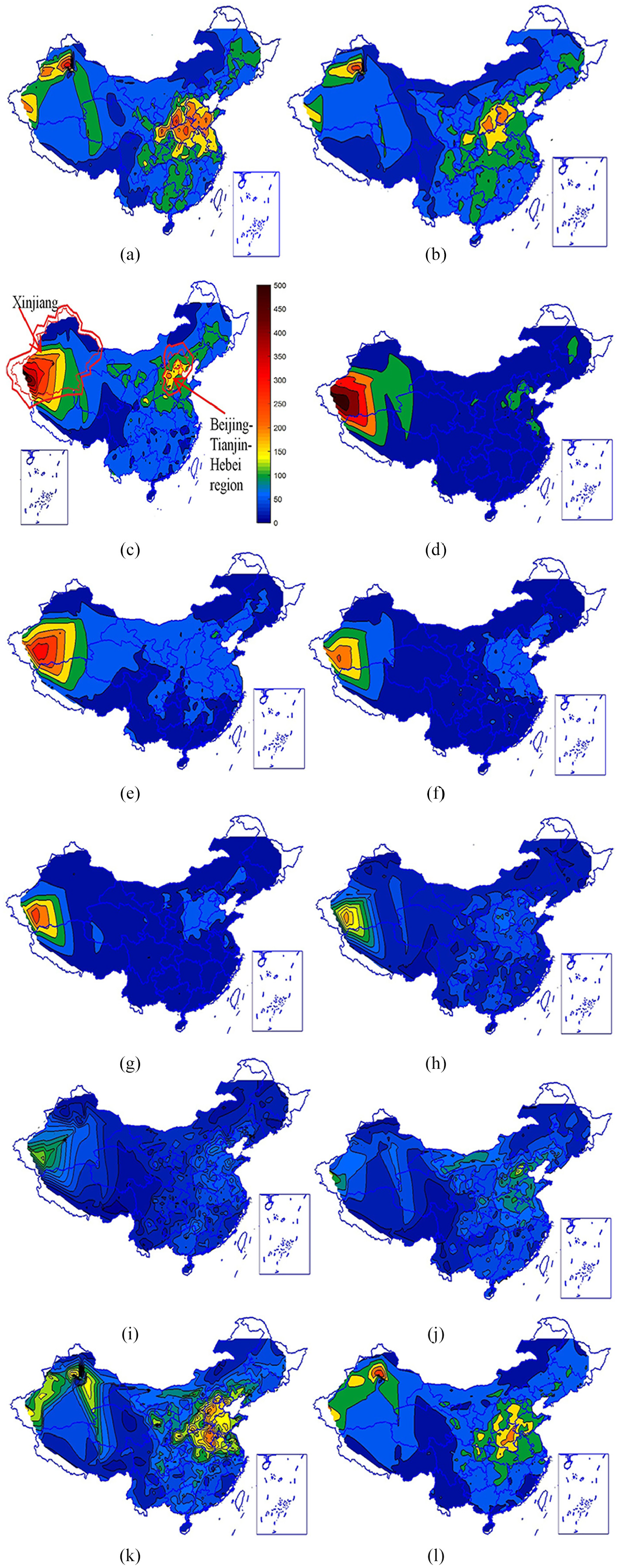
Monthly contour maps of the threshold across China’s national monitoring stations in 2018: (a) to (l) represent January to December, respectively.

Worth to notice that the Beijing–Tianjin–Hebei region (for its location, see Figure 1(c)) is one of the areas with higher thresholds. This phenomenon gives the following two implications: (1) the extreme haze is relatively severer in this region and (2) extreme haze often simultaneously occurred at many locations in this region, showing the so-called “extreme dependence” in the literature. The extreme haze problem in the Beijing–Tianjin–Hebei region is to be valued in that this region includes two national central cities out of nine, that is, Beijing (the capital of China) and Tianjin (the international shipping center of northern China and the economic center of Circum-Bohai Sea region). What’s more, it is one of the key regions in the “three-year plan on defending the blue sky.” In all, this article will focus on this region’s haze extreme co-movement by recognizing its extreme dependence patterns.

There are 13 cities in all in this region. Their locations are shown in Figure 2. Except for Beijing and Tianjin, 11 cities are included in Hebei province, which are Zhangjiakou, Chengde in the north of Hebei, Baoding, Langfang in the middle of Hebei, Qinhuangdao, Tangshan, and Cangzhou belong to the east of Hebei, and Shijiazhuang, Hengshui, Xingtai, and Handan in the south of Hebei. The number of monitoring stations in this region is rather stable during 2014–2018. Taking 2018 as an example, there are 12 stations in Beijing, 18 in Tianjin, and 51 in Hebei.

Figure 2.

The locations of cities in Beijing–Tianjin–Hebei region.

The monthly boxplot of the thresholds for stations in the Beijing–Tianjin–Hebei region from 2014 to 2018 is given in Figure 3. The extreme haze in 2014 is the worst out of 5 years since the quantiles in every month of 2014 are nearly the largest, however, becomes better in recent years. In January 2014, the thresholds of many stations are close to 500 μg/m³. When it came to the same month in 2018, the largest threshold decreases nearly a half to 272 μg/m³, showing significant improvement. As to the seasonality, the threshold shows relatively large mean and variance in the first and last quarter in all years, implying the high level and fluctuation of the PM2.5 level, that is, the severity of extreme haze during these two seasons. Specifically, March in 2018 and January in 2017 show higher means in the first quarter, while November in 2018 and December in 2017 are worse in the fourth quarter due to a similar reason.

Figure 3.

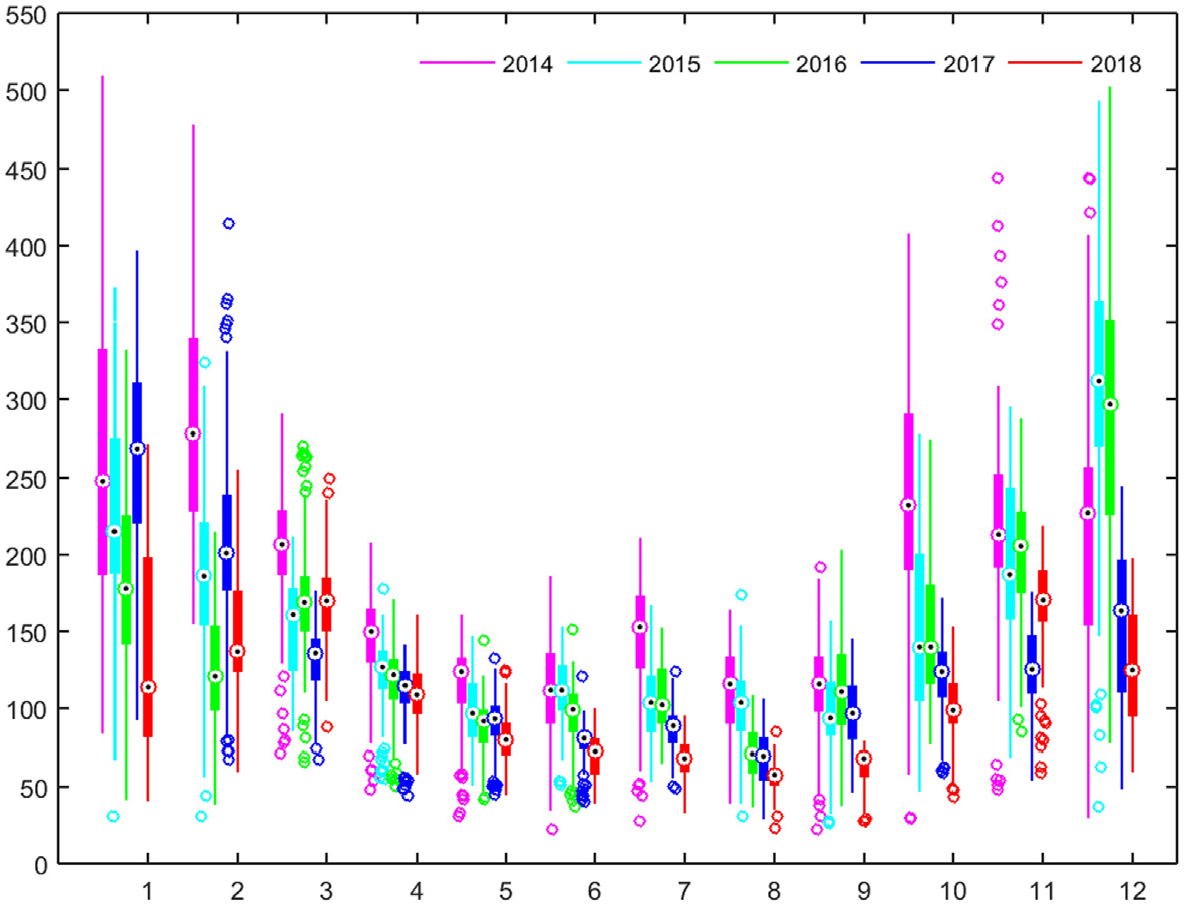
Boxplots of thresholds in the Beijing–Tianjin–Hebei region from 2014 to 2018.

The horizontal axis is the 12 months. The vertical axis is the threshold (μg/m³). For demonstration purpose, the thresholds larger than 550 μg/m³ are truncated. In each box plot, points are drawn as outliers if they are larger than q₃ + 1.5(q₃ − q₁) or smaller than q₁ − 1.5(q₃ − q₁), where q₁ and q₃ are the 25th and 75th percentiles, respectively. The 1.5 corresponds to approximately ±2.7σ and 99.3 coverage if the data are normally distributed. Besides, the black point in the colorful circle of each box represents the mean.

The monthly thresholds for each city are also calculated to give more results. Taking 2018 as an example, Figure 4 shows that the top four cities with the highest thresholds are Handan, Shijiazhuang, Xingtai, and Baoding, while the best three cities with relatively lower threshold are Qinhuangdao, Zhangjiakou, and Chengde.

Figure 4.

Monthly thresholds of stations in each city in 2018.

Assessing the extreme dependence of haze

As mentioned in the last section, the Beijing–Tianjin–Hebei region often suffers from heavy haze during the same period. The relationship between those extreme values of haze can be described by the approach of “tail dependence,” also known as “extremal dependence” or “asymptotic dependence,” which refers to the concurrence of extreme values between the components of a two-dimensional (2D) random vector.⁴⁷ Two identically distributed random variables X and Y with distribution function F are “tail independent,” if

λ = lim_{u \to x_{F}} P (Y > u | X > u)

(1)

is 0, where $x_{F} = sup {x \in R : F (x) < 1}$ . λ is called the bivariate tail dependence index, which quantifies the dependence of the bivariate upper tails. If λ > 0, we say that X and Y have “tail dependence,” that is, there are extreme co-movements between X and Y.

Worth to notice that tail dependence cannot be concerned as the probability of simultaneously observing extreme haze across all stations within a time window. It implies the conditional probability of observing extreme haze at s_i (for a particular station s_i, there is a station s_j) given extreme haze having been observed at s_j within a time window. For different station s_j, extreme haze may or may not be observed within that time window.

Statistical modeling of tail dependent variables has been a challenging task. It has been studied by many researchers, for example,^47–53 among many others. An alternative measure—the coefficient of tail dependence—was proposed by Ledford and Tawn;^50,51 it measures the dependence in asymptotic independence. The estimation of the coefficient of tail dependence is often model-based or non-parametrically estimated, which is not convenient when dealing with a large scale of variables, for example, hundreds of monitoring stations in this article. Zhang⁴⁸ introduced an empirically efficient test statistic, TQCC, for the null hypothesis of tail independence. The computations of TQCC do not need to jointly model paired random variables, that is, only marginally fitted distributions to exceedances are needed (comparable to computations of Pearson’s correlation coefficients); therefore, it is particularly appealing and used in this article. The definition of TQCC is as follows

The null hypothesis of tail independence is

H_{0} : λ = 0 and H_{1} : λ > 0

(2)

Suppose that ${(X_{i}, Y_{i})}_{i = 1}^{n}$ is a random sample of two unit Fréchet random variables (X, Y). The TQCC is defined as follows

q_{u_{n}} = \frac{max_{1 \leq i \leq n} {\frac{max (X_{i}, u_{n})}{max (Y_{i}, u_{n})}} + max_{1 \leq i \leq n} {\frac{max (Y_{i}, u_{n})}{max (X_{i}, u_{n})}} - 2}{max_{1 \leq i \leq n} {\frac{max (X_{i}, u_{n})}{max (Y_{i}, u_{n})}} \times max_{1 \leq i \leq n} {\frac{max (Y_{i}, u_{n})}{max (X_{i}, u_{n})}} - 1}

(3)

In Zhang et al.’s⁴⁹ work, the sequence of thresholds u_n is allowed to be a class of random variables and diverge to infinity in probability. This setting is more suitable to the practice, in which circumstance the data-driven thresholds to obtain extreme values are more commonly used compared with fixed thresholds.

It is also shown in Zhang et al.’s⁴⁹ work that the TQCC test statistics, under the null hypothesis of tail independence, follow the distribution of $2 n {1 - \exp (- 1 / u_{n})} q_{u_{n}} \overset{L}{\to} χ_{4}^{2}$ , where $χ_{4}^{2}$ is a chi-squared random variable with 4 degrees of freedom. The TQCC is also proved to be consistent under the alternative hypothesis of tail dependence under a general approximation of max-stable distribution.

For a given level α, if $2 n {1 - \exp (- 1 / u_{n})} q_{u_{n}} > χ_{4, α}^{2}$ , then H₀ of equation (2) is rejected, and we conclude that there exists tail dependence between two random variables of interest. Here $χ_{4, α}^{2}$ is the upper α percentile of the $χ_{4}^{2}$ distribution. If H₀ of equation (2) is rejected, then equation (3) can be used as an estimate of λ. In practice, we can simply choose u_n as the sample percentile, taking 95% used in this article, for example.

In equation (3), X and Y are supposed to be unit Fréchet random variables. This is not necessarily true in practice. Marginal transformation to the unit Fréchet distribution should be done to X and Y first. One way to obtain unit Fréchet scales is to fit the following generalized extreme value (GEV) distribution

H (x; ξ, μ, ψ) = \exp [- {\frac{1 + ξ (x - μ)}{ψ}}_{+}^{- 1 / ξ}]

(4)

to extreme values, where μ is a location parameter, ψ > 0 is a scale parameter, and ξ is a shape parameter. In principle, unit Fréchet scales can be obtained using the transformation −1/log{H(x; ξ, μ, ψ)}. Theoretical results⁴⁹ show that the TQCC calculated using the above transformation with estimated parameters of GEV distribution results in the same limiting distribution with the true parameters.

When fitting the GEV distribution, since the hourly data are not i.i.d. and show significant seasonality, as discussed in section “Data description,” the block maxima method to pick the extreme value and then fit the GEV distribution is not a good choice. In this article, instead, the marginal distribution of the exceedances of certain threshold (a typical 90% quantile is used in this article as mentioned in section “Data description”) along with the exceedance times is modeled via a Poisson-generalized Pareto distribution (GPD) process.The maximum likelihood function of this Poisson-GPD process shares the same parameters with the GEV distribution so that the maximum likelihood estimation (MLE) parameters in equation (4) can be derived. This approach is called the point process approach, see Coles⁵⁵ and Smith.⁵⁶

The temporal and spatial extreme dependence patterns of haze

In this section, the TQCC approach is used to disclose the extreme dependence of the haze between stations in the Beijing–Tianjin–Hebei region. The spatiotemporal patterns and the extreme co-movement of the haze are given.

TQCC calculation procedure

For each month, the TQCC between every station pair is conducted using equation (3) to take into account seasonality. When calculating TQCC, a time difference d between two data sets should be considered, since the tail dependence may not happen in the exactly same time window for two random variables but with a time difference. Specifically, in the case of d = 0, the TQCC describes the tail dependence of two stations that happened within the same time window, which is referred to as “simultaneous tail dependence,” denoted by q.

Considering that the average time duration of extreme haze in the Beijing–Tianjin–Hebei region is mostly equal or less than 3 days (since the extreme values used to calculate TQCC are those above the 90% quantile, the duration of extreme haze with the PM2.5 level larger than this threshold is naturally 3 days at most. This is because the meaning of the threshold is that at most one-tenth of the time per month (3 days) can experience the PM2.5 level exceeding the threshold), it is reasonable to set the maximum time difference to 48 h. Then, d is set to be integer hours ranging from −48 to 48, which covers 4 days. When d is positive or zero, the sample of s_i is set to be from the beginning of each month to 48 h before the end of the month, while for station s_j, the sample length is the same with s_i, but with d hours delay. This means that the time window of station s_i is d hour prior to station s_j, that is, the occurrence of extreme haze at s_i is prior to s_j. When d is negative, the samples of two stations exchange, implying that the time window of station s_i is d hour behind station s_j, that is, the occurrence of extreme haze at s_i is behind s_j.

Under the above procedure, the data sample of each station is 48 h shorter than a month and changes with d. Since it is assumed in this article that the extreme value distributions of all station are stationary in each month, it is reasonable that the estimated GEV parameters of the whole month rather than the real data sample are used when calculating TQCC to reduce the amount of computation. Besides, stations with estimated ξ larger than 1 or less than −1 are discarded to ensure a valid TQCC (or else it will be incorrectly insignificant or large).

Under the range of [−48, 48], there are 97 values of d and related TQCC in all. Significance tests are made for each TQCC using the chi-squared distribution. Then, the maximum TQCC denoted by maxq is selected among all the values, and the d corresponding to maxq is denoted by lagd.

The monthly variation of TQCC

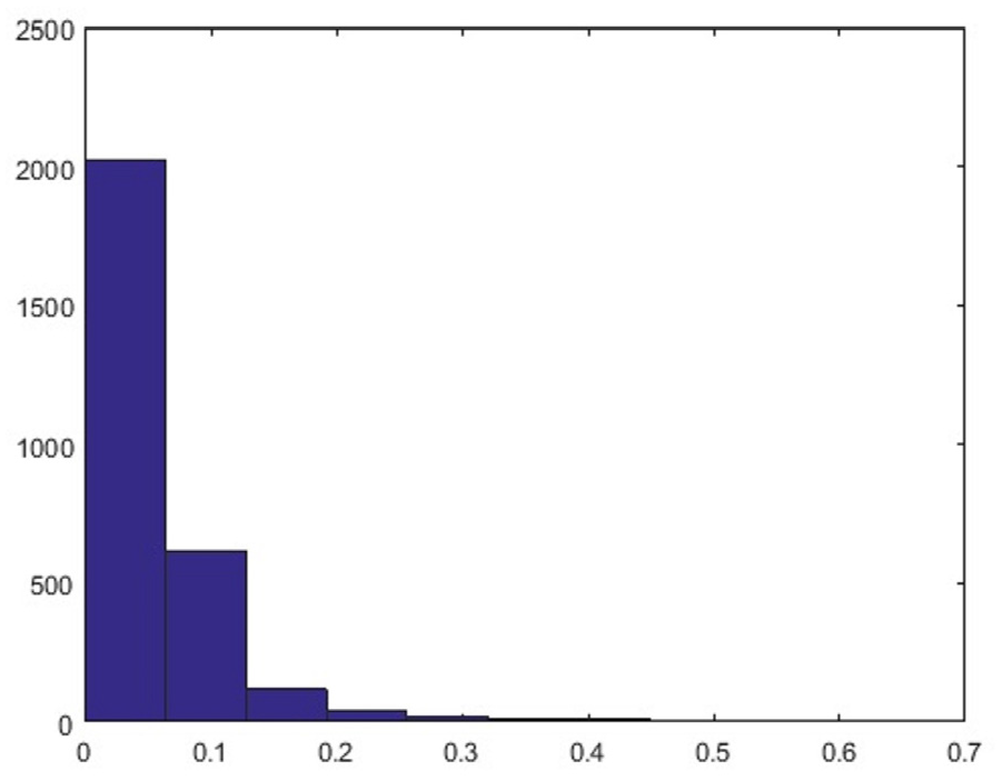
The TQCC between stations using the extreme values of the whole year is also calculated for comparison. The results show that the annual qs for each year from 2014 to 2018 are all chi-squared distributed but very small, implying that the annual average probability for the concurrence of extreme haze between stations is very small. Since haze is only extreme in a few months of the year, the longer the whole time range is, the smaller the average probability is. Taking 2018 for example, while the total station pairs in the Beijing–Tianjin–Hebei region are 3321, the frequency of station pairs with q equal to or larger than 0.1 is around 20, see Figure 5. When time difference d is considered, the maxq does not enhance much.

Figure 5.

Frequencies of paired annual q of 2018.

The monthly TQCC in 2018, by contrast, increases greatly compared with the annual ones. Even for the month with the smallest TQCC in 2018, that is, January, the frequency of station pairs with q equal to or larger than 0.1 exceeds 500, see Figure 6. The TQCCs increase in general with the month and become even higher in the last season. Taking the highest month November as an example, see Figure 7, most station pairs have their qs between 0.4 and 0.8, implying the high probability on the concurrence of extreme haze among stations. Considering that November is also one of the months suffering from the worst extreme haze due to its high threshold in 2018, the strong simultaneous extreme dependence in November will be studied further in section “The worst scenario 1: the concurrence of the worst extreme haze among and inside cities” to explore one of the worst scenarios, that is, the concurrence of the worst extreme haze between and inside cities.

Figure 6.

Frequencies of q of January 2018.

Figure 7.

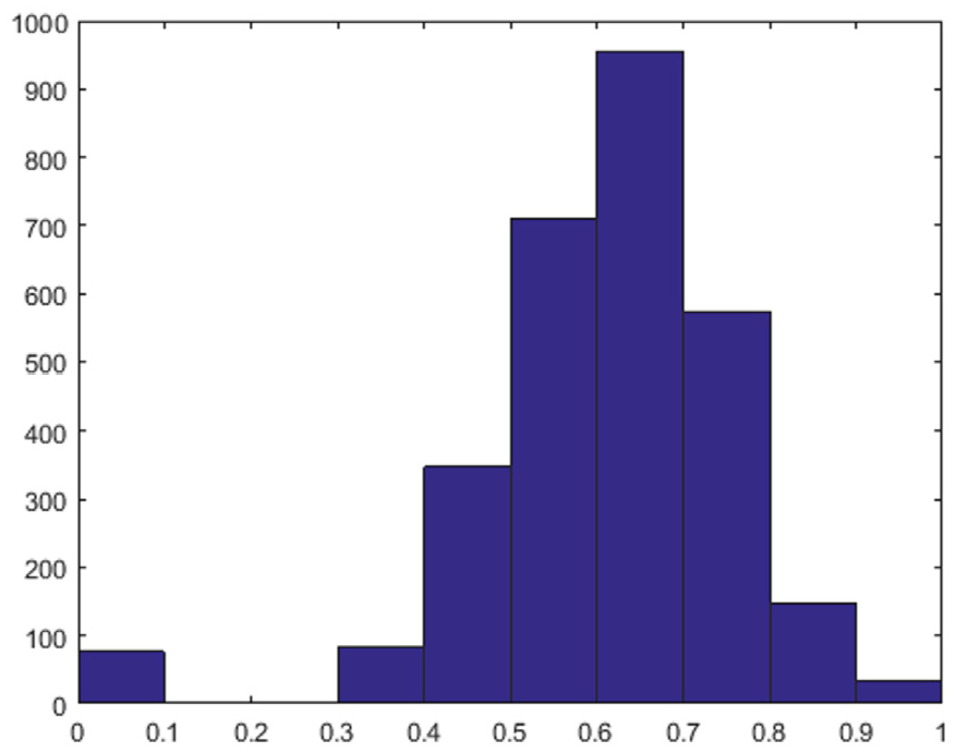
Monthly q of November 2018.

As to maxq in 2018, the values are not surprisingly larger than the monthly q in general. Worth to notice that with the increase in month, the maxq and q are not chi-squared distributed but having a high peak at large value away from zero. Taking November as an example, see Figures 7 and 8, the peak appears close to 0.7 for q, and to 0.8 for maxq. This observation clearly indicates that there exist tail dependences (i.e. extreme co-movements) among stations as under the null hypothesis of tail independence, one will observe a chi-squared like histogram pattern.

Figure 8.

maxq of November 2018.

The maxq and q in 2017 have similar features with 2018. They increase and appear peaks at large value as well with the month growing but reach the highest value in December.

Since TQCC is symmetric for station s_i and station s_j as shown in equation (3), the results of all station pairs can be represented by a triangular matrix. Graphs of these matrixes in March 2018 are made below to give visual demonstrations, see Figure 9. The principal diagonal of the triangular matrix is not shown on the graph since it represents the self-tail dependence of one station and equals to 1.

Figure 9.

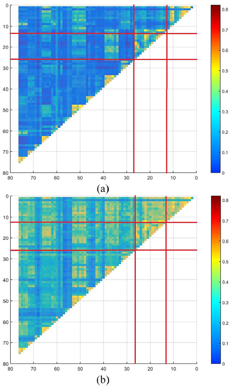
Triangular matrix graphs of maxq (a) and q (b) between stations in March 2018. Stations 1–12 belong to Beijing; Stations 13–27 belong to Tianjin (Two stations have been deleted due to large amount of zeros), the others belong to Hebei. They are blocked with red lines.

Some extreme dependence pattern can be concluded. Generally speaking, in all months, simultaneous extreme dependence qs between station pairs inside every single city, especially Beijing and Tianjin are significantly larger than those cross cities. These qs with d = 0 are usually the largest among all the value of d. Taking March as an example, the larger qs inside cities in Figure 9(a) are equal to its related maxq in Figure 9(b). This observation implies a large probability on the concurrence of extreme haze between stations inside cities.

In August, qs between station pairs across Beijing and Tianjin are large as well. In October, the qs between most stations of Beijing and other stations are close to 1. These 2 months are the typical cases on the concurrence of extreme haze between stations across cities.

When a time difference d is considered, the extreme dependence between stations across cities is universally high. Taking March as an example, as shown in Figure 9(a), the maxq between stations across cities enhanced generally, although the simultaneous extreme dependence in March is not very strong. This implies the existence of time difference on the extreme haze’s appearance. Since March is one of the months suffering from the worst extreme haze due to its high threshold as mentioned before, the existence of time differences in March 2018 is especially interesting in that it represents another worst scenario, that is, the lag effects of the worst extreme haze’s occurrence (with the largest probability) between different locations. We will study this worst scenario in section “The worst scenario 2: the lag effects of the worst extreme haze’s occurrence.”

The worst scenario 1: the concurrence of the worst extreme haze amongand inside cities

As it can be seen from the last section, simultaneous tail dependence between stations does exist inside the Beijing–Tianjin–Hebei region. Strong tail dependence station pairs could be listed to give more specifications. However, those station pairs are too small as a unit for the government to make policies. In this section, certain criterions are given to select strong enough simultaneously extreme dependence cities. November 2018, with the top thresholds and largest simultaneous extreme dependence, will be taken as an example to analyze the concurrence of the worst extreme haze among and inside cities. The selection criterions are as follows:

Step 1: TQCC selection. Find all the q greater than or equal to certain threshold qTsh. This can ensure the strong enough tail dependence between station pairs.

Step 2: city identification. Among all those selected q, each one is identified and classified that whether this q belongs to two stations inside the same city (named as a single city) or between two cities (named as one city pair).

Step 3: ratio calculation. For every single city and city pair, count how many q being greater than or equal to the qTsh. The ratios of the amount of selected q to the number of total pairs inside every single city or between city pair are calculated. The ratio equals to 1 means that all the station pairs inside a single city or between city pair have the q greater than or equal to qTsh.

Step 4: city selection. Select all of those single cities and city pairs (named as selected single cities and selected city pairs) that have a ratio greater than or equal to certain threshold rTsh. This can ensure enough amounts of strong extreme dependence between stations, no matter how many selected q is (q usually varies largely among single cities and city pairs).

The selected single cities or selected city pairs indicate those cities with very large probability suffering extreme haze simultaneously. Given different (qTsh, rTsh), the results of selected single cites and city pairs (along with how many cities involved) are shown in Table 1.

Table 1.

Results of selected single cites and city pairs under different (qTsh, rTsh).

	Number of selectedcity pairs (amount of cities involved)			Number of selected single cities			Number of selectedcity airs (amount ofcities involved)			Number of selectedsingle cities			Number of selected city pairs(amount of citiesinvolved)			Number of selected single cities
qTsh	0.5			0.5			0.6			0.6			0.7			0.7
rTsh	0.5	0.6	0.7	0.5	0.6	0.7	0.5	0.6	0.7	0.5	0.6	0.7	0.5	0.6	0.7	0.5	0.6	0.7
Results	72 (13)	70 (13)	60 (13)	12	12	12	46 (13)	36 (12)	30 (11)	12	12	11	15 (9)	8 (8)	3 (3)	11	11	10

Under all the given (qTsh, rTsh) in the table, the selected single cites include almost all cities. Even for the highest value (0.7, 0.7) in the table, the number is still 10. This implies a high probability of concurrence of extreme haze inside one city. This is not surprising since most stations are located closely in downtown. As to the selected city pairs, they vary mainly with qTsh rather than rTsh. They cover all the cities in the case of qTsh = 0.5, with the number of selected city pairs nearly amounts to 80% of the whole pairs (91 pairs in all) no matter what rTsh is, showing universal high extreme dependence among stations across cities. In the case of qTsh = 0.6, the selected city pairs still involve almost all the cities, only the amounts drop a half, which is still not clear enough to conclude. The case of qTsh = 0.7 will be analyzed in detail due to its strong extreme dependence level (the TQCC ≥ 0.8 is very rare between stations). Typical results are given under (qTsh = 0.7, rTsh = 0.5), in which case, the number of selected city pairs is 15 and involves 9 cities.

Among these selected city pairs, 6 out of 15 (the most occurrence) involve Baoding city, which is the most frequently extremal co-movement city with others. This implies that when the extreme haze appears in Baoding, there is a large probability that the extreme haze also appears in other six cities at the same time.

As to paired cities, among Baoding, Tianjin, and Langfang, every two of them are included in the selected city pairs, which imply that once extreme haze happens in one of these cities, the other two cities will also suffer from extreme haze simultaneously with high probability. This group of cities can be named as concurrent city cluster. Notice that these three cities are adjacent so that they are very naturally to form a city cluster or network. The second concurrent city cluster includes four cities, namely, Tangshan, Tianjin, Baoding, and Xingtai. The third concurrent city cluster is Tangshan, Handan, and Xingtai. Moreover, 85% of station pairs between Tangshan and Xingtai have extreme dependence larger than 0.7. The ratio is the largest one among city pairs and implying the most closely extreme co-movement between these two cities. The locations of three concurrent city clusters are drawn in Figure 10 using different colors.

Figure 10.

Three concurrent city clusters.

Notice that Shijiazhuang is not included in the second concurrent city cluster, although it is adjacent to the cluster. This observation implies that the probability that Shijiazhuang suffers from simultaneous extreme haze with this city cluster is not very large but possibly with a time difference. Specifically, from the sign of lagd between stations cross Shijiazhuang and cities in the cluster, we can tell that the occurrence of extreme haze in Shijiazhuang is posterior to the city cluster. Considering that Shijiazhuang has a higher threshold of extreme haze than the cities in the cluster in November as shown in Figure 4, one possible explanation is that when the extreme haze covering all these cities, the PM2.5 level of the city cluster is not the extreme value for Shijiazhuang yet. With the time passing a few hours, the PM2.5 level in Shijiazhuang will rise to a higher level.

Similarly, the third concurrent city cluster does not include Cangzhou and Hengshui, although they are connected. On one hand, the signs of lagd between them demonstrate that most stations in the two cities are prior to cities in this cluster. On the other hand, Cangzhou and Hengshui have similar lower threshold of extreme haze than the third city cluster as shown in Figure 4; one potential conclusion is that when PM2.5 in Hengshui and Cangzhou approaches to the extreme value with the occurrence of haze, the PM2.5 level in the third city cluster will go even higher in a few hours.

The results of 2017 are also made for comparison. In the same month of 2017, it shares the same city pair Tangshan and Xingtai that has the largest rTsh (equal to 1 this time), that is, implying the most closely extreme co-movement between them. Moreover, city pairs of Tianjin and Tangshan and Tianjin and Baoding included in city clusters in this month are shared by both years. Only that the simultaneous extreme dependence in November 2017 is slightly lower than the same period of 2018 that the above results exist under the condition of qTsh = 0.6 and rTsh = 0.5 in 2017.

Considering that the qs in December are the largest of 2017 while the thresholds of extreme value are the highest in the fourth quarter; the results of December 2017 are also given to show the same worst scenario as in November 2018. It shows that three city pairs, that is, Tianjin and Tangshan, Tianjin and Langfang, and Handan and Xingtai belonging to city clusters are shared in both worst scenarios.

The similarity between November and December 2017 shows that the extreme co-movement of haze in the fourth quarter has certain regular patterns. So does the same month of 2017 and 2018.

The worst scenario 2: the lag effects of the worst extreme haze’s occurrence

This section will take March 2018 as an example to illustrate another worst scenario of extreme haze, that is, when the extreme haze is very severe, the concurrence of extreme haze exists a time difference. It is shown from Figure 11 that the lagd has an approximately symmetric distribution with its highest peak falling into interval [−10, 0].

Figure 11.

lagd of March 2018.

The following criterion is used to select single cities and city pairs that have enough station pairs with the lagd belonging to certain intervals of time differences. Considering the maximum time difference is 48 h, four kinds of intervals are considered, that is, within 6 h, 6–12 h, 12–24 h, and 24–48 h:

Step 1: lagd selection. Find all the lagd that falling into four intervals of dTsh, respectively.

Step 2: city identification. For each interval of dTsh, two stations related to each selected lagd are identified and classified as long as they belong to a single city or a city pair.

Step 3: ratio calculation. For each interval of dTsh, calculate the ratio of the number of selected lagd to the total number of station pairs inside every single city or between city pairs.

Step 4: city selection. Selected single cities and selected city pairs are those that have the ratio greater than or equal to certain threshold rTsh. The ratio here can be explained as the probability of the extreme haze’s appearance within a certain time difference. Therefore, these selected cities have a large probability that the concurrence of extreme haze exists a certain time difference.

Table 2 gives the result on different (dTsh, rTsh) in March to demonstrate the lag effects of extreme haze.

Table 2.

Result of selected single cites and city pairs under different (dTsh, rTsh).

	Total number of selected city pairs(total number of cities involved)		Number ofselected single cities		Total number ofselected city pairs(total number of cities involved)		Number ofselectedsingle cities		Total number ofselected city pairs(total number ofcities involved)		Number ofselectedsingle cities		Total numberof selectedcity pairs(total number of cities involved)		Number of selected single cities
dTsh	[−6, 6]		[−6, 6]		[−12, −6),(6, 12]		[−12, −6),(6, 12]		[−24, −12),(12, 24]		[−24, −12),(12, 24]		[−48, −24),(24, 48]		[−48, −24),(24, 48]
rTsh	0.5	0.7	0.5	0.7	0.5	0.7	0.5	0.7	0.5	0.7	0.5	0.7	0.5	0.7	0.5	0.7
	16 (13)	10 (11)	13	13	10 (10)	6 (7)	0	0	24 (13)	17 (13)	0	0	16 (11)	11 (8)	0	0

As far as the selected single cities are concerned, all the cities are involved in the interval of [−6, 6], and none falls into other intervals. This phenomenon implies that there is a high probability that stations inside one city are extremely dependent within 6 h since most stations are closely located in downtown. As to the selected city pairs, however, they fall into different intervals of dTsh, implying the existence of varying time difference. Specifically, when rTsh is 0.5, the numbers of cities involved in different intervals of dTsh are all larger than 10. While the ratio of station pairs between two cities enhanced to 0.7, the cities involved in selected city pairs decreased to some extent and showed more clear relations as follows.

There are ten selected city pairs falling into the interval of [−6, 6]. As far as Baoding, Beijing, and Langfang are concerned, any two of them are included in the selected city pairs. This phenomenon implies that there is a large probability that once extreme haze occurred in any one city, the other two cities will suffer extreme haze within 6 h. This kind of city group can be named as the 6-h city cluster, which is shown in Figure 12. It is very intuitive for this city cluster having the lagd within 6 h since they are adjacent. Especially, the rTsh between Baoding and Langfang is 1, meaning all of the station pairs between these two cities have the lagd falling into [−6, 6]. They are the most closely co-movement cities.

Figure 12.

City pair and city clusters with certain time difference.

There are six selected city pairs falling into the interval of [−12, −6),(6, 12]. All the station pairs between Baoding and Tangshan satisfy this time interval, and the locations of this city pair are demonstrated in Figure 12. They are the most closely co-movement within this time difference. There does not exist a city cluster within this time interval (no city cluster in the interval of [−48, −24),(24, 48] either).

There are 17 selected city pairs falling into the interval of [−24, −12),(12, 24], among which both Baoding and Hengshui are involved five times separately. They are the most frequently extreme dependent cities with others. In addition, Baoding, Handan, and Hengshui group as a 12- to 24-h city cluster, which is shown in Figure 12. Specifically, all the station’s pairs between Baoding and Hengshui satisfy this time interval. This most closely co-movement city pair includes Baoding once again.

In all, Baoding city is the most frequently extreme co-movement city with others in that it is repeatedly included in all city clusters and has the 100% station pairs with other city falling into all the time intervals. Baoding shows different time difference patterns with other cities during the worst extreme haze in March.

Moreover, except the specific value of lagd, its sign is also important as it represents the precedence order of the extreme haze’s occurrence, as mentioned in section “TQCC calculation procedure.” In March, all the stations in Tianjin, Tangshan, Qinhuangdao, Cangzhou, and Hengshui (March 2017 are the same except for Hengshui) are prior to stations in Beijing on the extreme haze’s occurrence (with large probability since the related maxq is high). The locations of these cities and the order are shown in Figure 13(a). Qinhuangdao, however, has the large probability that the occurrence of extreme haze at almost all its stations is prior to other cities (except for Zhangjiakou, Cangzhou, and Hengshui in March 2018 and prior to all the other cities in March 2017), see Figure 13(b).

Figure 13.

Precedence orders on the extreme haze’s occurrence in March 2018. (a): Cities with stations prior to stations of Beijing. (b): Cities with stations after stations of Qinhuangdao. The city A points to B by an arrow which represents that the appearance of extreme haze inA has an earlier time window than B.

All the stations of Cangzhou and Hengshui are prior to other cities in March (similar to November as mentioned before). As to the precedence orders on the extreme haze’s occurrence between Beijing and other cities in other months, however, things are changed in January 2018 (except Tangshan and Zhangjiakou) when the occurrence of extreme haze (with a large percent of stations) in most cities is behind Beijing.

Conclusion and discussion

This article employs the novel approach TQCC to disclose the extreme dependence patters of haze in the Beijing–Tianjin–Hebei region. By utilizing the hourly PM2.5 data from monitoring stations across the whole region during 2014–2018, the spatial and temporal variation of haze’s extreme dependence is given. Then two special worst scenarios, the concurrence of the worst extreme haze among and inside cities, and the lag effects of the worst extreme haze’s occurrence are analyzed, from which concurrent city clusters, city clusters with the certain time difference, and the precedence orders of the extreme haze’s occurrence are identified. The above analyses give informative results on the haze’s extreme co-movements and draw different conclusions and implications compared with prior works.

However, this article focuses on the extreme haze rather than the average haze, while other extensive papers analyze the haze in single cities with the average PM2.5 data (Typical results on the high polluted areas are similar with the high threshold cities in our article.^39,40,57,58). Not only that, this article investigates the extreme dependence of the haze across different locations. Among the few works that concern the co-movement rather than its extreme co-movement of the haze, the spatial dependence of PM2.5 among cities was explored via spatial autocorrelation analysis.^35–37 It demonstrates that the period with severe haze (e.g. winter) also shows strong spatial dependence, so does the cities with severe haze (Shijiazhuang and Hengshui). The spatial autocorrelation describes the dependence of PM2.5 level among different locations mainly using the centralized data in the middle part as most commonly used coefficients do. In contrast, TQCC describes the probability that extreme haze appears at one location when it has been observed at another location within a certain time window. Moreover, the results of this article show that the period with severe haze (high threshold) and the one with strong TQCC are not coincident, which exactly provide two interesting and discussable scenarios and lead to informative results as follows.

First, from January to December, the TQCC in 2017 and 2018 shows more and more high values, that is, the co-movements of extreme haze increase with the changing months. Interestingly, in the fourth season, the haze is relatively severe, and the simultaneous extreme dependence is strong. The typical feature of this scenario is the concurrence of the worst extreme haze. In the first season, the haze is also severe while the extreme co-movement with a certain time difference is much stronger than the simultaneous extreme dependence (much lower than the fourth season). This observation represents another scenario that the occurrence of the worst extreme haze exists time difference.

This article analyzes the spatial pattern of stations inside and between cities under the above two worst scenarios, taking typical months of 2017 and 2018 as an example. The results show that the probability that stations inside single cities (especially Beijing and Tianjin) suffer extreme haze simultaneously or within 6 h is relatively higher due to the dense distribution of most stations in downtown inside one city. As to the extreme co-movement between cities, certain common conclusions under the worst scenario 1 are drawn in 2017 and 2018 since several selected city pairs are shared by both years during the same or closed month. The concurrent city clusters, among which any two cities suffered from simultaneous extreme haze with large probability, are identified. We strongly suggest that the government performs joint prevention and control measurement on cities in the concurrent city clusters considering their large probability on the concurrence of extreme haze.

It is interesting to notice that although some cities connect with the concurrent city cluster, the simultaneous extreme dependences between them are not large enough. Further analysis shows that the city with extreme haze’s appearance posterior to the adjacent city cluster, Shijiazhuang, for example, has a higher threshold than the adjacent city cluster, showing relatively severer extreme haze. While cities with the extreme haze’s occurrence prior to the adjacent city cluster, taking Cangzhou and Hengshui for example, often have a lower threshold than the adjacent city cluster, showing relatively weaker extreme haze. In other words, among these adjacent cities, the extreme haze with earlier appearance is usually less severe than the one with the later appearance. Considering the generally high simultaneous extreme dependence during this month, the possible cause is that the extreme haze does appear in all these adjacent cities at the same time. However, the pollutants further accumulate in certain cities which lead to continuously increasing PM2.5 level and higher extreme values in these cities a few hours later. The route of the PM2.5 level’s rise and its cause of formation should be paid attention to, and target actions should be taken.

Among all the cities, Baoding, with its location in the middle of Hebei province, is the most frequently extreme co-movement city with others. In other words, when other cities suffered extreme haze, there is a large probability that the extreme haze will appear in Baoding within some time window, and vice versa. The frequent arrivals of extreme haze are probably one big reason that Baoding suffered severe haze (high threshold) in the whole region. Although research shows that the cumulated PM2.5 decrease in Baoding during the recent 5 years is the largest in the Beijing–Tianjin–Hebei region,⁵⁸ it is worth to notice that its extreme haze is still severe. For example, in November, the month with the strongest simultaneous extreme co-movement of haze, the probability on the concurrence of extreme haze in Baoding and other six cities is so high that Baoding is included in two concurrent city clusters. While in March, the typical month of the worst scenario 2, Baoding’s frequent extreme co-movement with other cities shows that the time difference of Baoding with the adjacent Langfang and Beijing is within 6 h and the one of Baoding with Tangshan in its east is 6–12 h, with Hengshui and Handan in its south is 12–24 h.

Except for its problems (Baoding locates along the Taihang Mountain, where the diffusion conditions are constraint by the geographical factors), Baoding connects cities of the Beijing–Tianjin–Hebei region in three directions (south, north, and east) so that it may be affected by these cities easily, for example, suffered from the transmission of PM2.5 from other cities.³⁵ As such, it may be the reason why Baoding has strong extreme co-movement with other cities and suffered from extreme haze repeatedly, which shows the necessity of joint governance and control in the Beijing–Tianjin–Hebei region.

The importance of lag effects is also reflected in the precedence order of the extreme haze’s appearance. In March 2018 and the same period of 2017, the time window of extreme haze’s appearance in Tianjin, Tangshan, Qinhuangdao, and Cangzhou is all earlier than Beijing. Since these cities are all located in the east and south of Beijing, the south or southwest winds that begin to rise in March may blow the pollution emissions from other cities to Beijing.²⁴ However, the occurrence of extreme haze in Qinhuangdao is prior to most or even all the cities, that is, when the extreme haze appears in Qinhuangdao, there is a large probability that the extreme haze will appear in other cities soon. This empirical result gives great implications that attention should be paid on the occurrence of extreme haze in Qinhuangdao to activate the early warning.

In January, however, the extreme haze’s appearance in Beijing is prior to most of the other cities. This is possibly related to the frequently occurring north or northeast wind. Due to the potential delivery of pollutant from Beijing to the city in its east and south with the aid of wind,²⁵ the PM2.5 level of cities in the leeward location will rise correspondingly and approaches the extreme value with a few hours’ lag. We suggest that the appearance of extreme haze in Beijing be paid close attention to, which implies that other cities will suffer extreme haze very soon with a large probability. This will greatly help the forecast of extreme haze in the Beijing–Tianjin–Hebei region.

There may be some common reasons for the precedence order of the extreme haze’s appearance mentioned above. Considering the facts that the probability on the concurrence of extreme haze among cities in January and March is relatively low, it is possible that the haze occurred first in some of the cities, when the PM2.5 levels in other cities are not very high yet but rise greatly later with the transmission of pollutant.^36,37 Different from the previous case of the concurrent city cluster and its adjacent cities, the extreme PM2.5 value in the cities with the extreme haze’s late occurrence is not necessarily higher than the city with the extreme haze’s early occurrence.

In all, as to the measures targeting extreme haze in the Beijing–Tianjin–Hebei region, joint prevention and control should be performed to the cities, especially in the concurrent city cluster and the most frequently extremal co-movement cities. The results of this article have strong implications for improving “the joint prevention and control on the atmospheric pollution in the Beijing–Tianjin–Hebei region and its surrounding key areas” in the national strategy since not only extreme haze in individual cities should be modeled, but the co-movement and relations between cities should also be taken into consideration.

Meanwhile, as a joint interprovincial haze control case, although Beijing, Tianjin, and Hebei province have set up unified haze early warning standard, early warning mechanism should also be hierarchical with certain hours of lags. Specifically, the activation mechanism should take into account the precedence order of extreme haze and be activated by the first appearance of extreme haze. The precedence orders also benefit the haze forecasting. On one hand, the precedence order and specific time differences can help to give a more precise forecast on the time point of the extreme haze’s occurrence in a direct way. On the other hand, it avails the investigation on the transmission path of the haze, based on which more precise meteorological models can be made to benefit the forecasting of the PM2.5 concentration.

The co-movement pattern between stations can also help advance the simultaneous haze control network inside the city and benefit the establishment of the haze monitoring stations inside the city as well, which could be discussed in our future work. Finally, we remark that extreme value analysis has been widely applied to climate studies, including extreme haze problems, that is, the references given in this article and those in Zhang et al.⁴⁹ We adopt TQCC approach in this study due to its easy computability in equation (3), interpretability,^48,49 and its complementary property to the linear correlation coefficient as shown in Zhang et al.⁵⁹ that TQCC and the sample-based linear correlation coefficient are asymptotically independent. We only focus on evaluating the tail relationship of haze values among the chosen stations in the Beijing–Tianjin–Hebei region. One can certainly apply other advanced methods in the literature, for example, those discussed in Zhang et al.,⁴⁹ to study the relationship of extreme haze. We note that evaluating variable relations is very common in the literature, for example, Zhang et al.⁴⁹ studies the tail dependence of heavy precipitations in the continental US, and numerous papers study economic variable relationships, social network relationships, and gene relationships among thousands of genes using linear correlation coefficient. One can certainly consider jointly modeling extreme haze among all stations (even involving spatial statistics). We shall leave this task in different projects.

Footnotes

Declaration of conflicting interests

The author(s) declared no potential conflicts of interest with respect to the research, authorship, and/or publication of this article.

Funding

The author(s) disclosed receipt of the following financial support for the research, authorship, and/or publication of this article: This work was supported by the MOE (Ministry of Education in China) Project of Humanities and Social Sciences (grant no. 19A10034014) and the Disciplines Funds of Central University of Finance and Economics.

ORCID iD

Lu Deng

Author biographies

Lu Deng, Professor in School of Statistics and Mathematics, Central University of Finance and Economics, Beijing, China, research area is extreme value and time series modeling.

Zhengjun Zhang, Professor in Department of Statistics, University of Wisconsin Madison, Madison, WI, USA, research area is extreme value analytics for big data, risk analysis, and nonlinear/asymmetric causal inference.

References

Hidy

GM.

An historical experiment: Los Angeles smog evolution observed by blimp. J Air Waste Manag Assoc 2018; 68(7): 643–655.

Jacobs

Burgess

Abbott

MB.

The Donora smog revisited: 70 years after the event that inspired the clean air act. Am J Public Health 2018; 108(S2): S85–S88.

Zhang

Liu

BJ.

Tackling air pollution in China-what do we learn from the great smog of 1950s in London. Sustainability 2014; 6: 5322–5338.

Fanizza

De Berardis

Ietto

, et al. Analysis of major pollutants and physico-chemical characteristics of PM2.5 at an urban site in Rome. Sci Total Environ 2018; 616–617: 1457–1468.

Romano

Perrone

Pavese

, et al. Optical properties of PM2.5 particles: results from a monitoring campaign in southeastern Italy. Atmos Environ 2019; 203: 35–47.

Sahu

Pervez

Chow

, et al. Temporal and spatial variations of PM2.5 organic and elemental carbon in Central India. Environ Geochem Health 2018; 40(5): 2205–2222.

Chowdhury

Dey

Smith

KR.

Ambient PM2.5 exposure and expected premature mortality to 2100 in India under climate change scenarios. Nat Commun 2018; 9(1): 318.

Ashraf

Butt

Khalid

, et al. Smog analysis and its effect on reported ocular surface diseases: a case study of 2016 smog event of Lahore. Atmos Environ 2019; 198: 257–264.

Cyranoski

China tests giant air cleaner to combat smog. Nature 2018; 555: 152–153.

10.

Yang

Zhong

NS.

Effect on health from smoking and use of solid fuel in China. Lancet 2008; 372(9648): 1445–1446.

11.

Liu

Han

Tang

, et al. Estimating adult mortality attributable to PM2.5 exposure in China with assimilated PM2.5 concentrations based on a ground monitoring network. Sci Total Environ 2016; 568: 1253–1262.

12.

Guo

Wang

Zhang

, et al. The association between ambient PM2.5 exposure and the risk of preterm birth in China: a retrospective cohort study. Sci Total Environ 2018; 633: 1453–1459.

13.

Shou

Huang

Zhu

, et al. A review of the possible associations between ambient PM2.5 exposures and the development of Alzheimer’s disease. Ecotoxicol Environ Saf 2019; 174: 344–352.

14.

Zhou

Chen

Tian

The impact of fine particulate matter (PM2.5) on China’s agricultural production from 2001 to 2010. J Clean Prod 2018; 178: 133–141.

15.

Pearce

Morrison

, et al. Up in smoke? The impact of smog on risk perception and satisfaction of international tourists in Beijing. Int J Tour Res 2016; 18(4): 373–386.

16.

Zhang

Would smog lead to outflow of labor force? Empirical evidence from China. Emerg Mark Financ Tr 2017; 53(5): 1122–1134.

17.

You

Liu

Dai

, et al. BP neural network-based smog environment and the risk model of mood driving. Appl Ecol Env Res 2017; 15(3): 1753–1763.

18.

Cao

Rao

, et al. Improving the electrospinning process of fabricating nanofibrous membranes to filter PM2.5. Sci Total Environ 2019; 666: 1011–1021.

19.

Fang

Zhang

, et al. New two-step extraction method in antimony speciation using HPLC-ICP-MS technique in inhalable particulate matter (PM2.5). Microchem J 2019; 146: 1269–1275.

20.

Antony Chen

Cao

. PM2.5 source apportionment using a hybrid environmental receptor model. Environ Sci Technol 2018; 52(11): 6357–6369.

21.

Saraga

Tolis

Maggos

, et al. PM2.5 source apportionment for the port city of Thessaloniki, Greece. Sci Total Environ 2019; 650(Pt. 2): 2337–2354.

22.

Pimonsree

Vongruang

Impact of biomass burning and its control on particulate matter over a city in mainland Southeast Asia during a smog episode. Atmos Environ 2018; 195: 196–209.

23.

Timmermans

Kranenburg

Manders

, et al. Source apportionment of PM2.5 across China using LOTOS-EUROS. Atmos Environ 2017; 164: 370–386.

24.

Yang

Yuan

, et al. The relationships between PM2.5 and meteorological factors in China: seasonal and regional variations. Int J Environ Res Public Health 2017; 14(12): 1510–1520.

25.

Zhang

LP.

Multifractal detrended cross-correlation analysis between PM2.5 and meteorological factors. Physica A 2015; 438: 114–123.

26.

Belle

Wang

, et al. Impacts of snow and cloud covers on satellite-derived PM2.5 levels. Remote Sens Environ 2019; 221: 665–674.

27.

Cao

Kostka

Environmental political business cycles: the case of PM2.5 air pollution in Chinese prefectures. Environ Sci Policy 2019; 93: 92–100.

28.

Wang

Zhu

, et al. Concentration distribution and control strategy of indoor PM2.5. Procedia Eng 2017; 205: 1606–1611.

29.

van Donkelaar

Martin

Brauer

, et al. Use of satellite observations for long-term exposure assessment of global concentrations of fine particulate matter. Environ Health Perspect 2015; 123(2): 135–143.

30.

Bhardwaj

Pruthi

Variability analysis in PM25 monitoring. Data Brief 2019; 24: 103774.

31.

Guo

Cheng

, et al. Assessment of PM2.5 concentrations and exposure throughout China using ground observations. Sci Total Environ 2017; 601–602: 1024–1030.

32.

Gui

Che

Wang

, et al. Satellite-derived PM2.5 concentration trends over Eastern China from 1998 to 2016: relationships to emissions and meteorological parameters. Environ Pollut 2019; 247: 1125–1133.

33.

Liang

Zou

Guo

, et al. Assessing Beijing’s PM 2.5 pollution: severity, weather impact, APEC and winter heating. Proc R Soc A 2015; 471: 0257.

34.

Zhang

, et al. Asymmetric multifractal detrending moving average analysis in time series of PM2.5 concentration. Physica A 2016; 457: 322–330.

35.

Jin

Fang

Wen

, et al. Spatio-temporal variations of PM2.5 emission in China from 2005 to 2014. Chemosphere 2017; 183: 429–436.

36.

Yan

Lei

Shi

, et al. Evolution of the spatiotemporal pattern of PM2.5 concentrations in China: a case study from the Beijing-Tianjin-Hebei region. Atmos Environ 2018; 183: 225–233.

37.

, et al. Routes and clustering features of PM2.5 spillover within the Jing-Jin-Ji region at multiple timescales identified using complex network-based methods. J Clean Prod 2019; 209: 1195–1205.

38.

Wang

Zhu

Guo

, et al. The heterogeneous effect of democracy, political globalization, and urbanization on PM2.5 concentrations in G20 countries: evidence from panel quantile regression. J Clean Prod 2018; 194: 54–68.

39.

Zhang

Shuai

Bian

, et al. Socioeconomic factors of PM2.5 concentrations in 152 Chinese cities: decomposition analysis using LMDI. J Clean Prod 2019; 218: 96–107.

40.

Yao

Long

XL.

What causes PM2.5 pollution? Cross-economy empirical analysis from socioeconomic perspective. Energ Policy 2018; 119: 458–472.

41.

Zhao

Wang

Niu

, et al. Red warning for air pollution in China: exploring residents’ perceptions of the first two red warnings in Beijing. Environ Res 2018; 161: 540–545.

42.

Ban

Zhou

Zhang

, et al. The health policy implications of individual adaptive behavior responses to smog pollution in urban China. Environ Int 2017; 106: 144–152.

43.

Qin

Wang

SY.

Young people’s behaviour intentions towards reducing PM2.5 in China: extending the theory of planned behaviour, resources. Resour Conserv Recy 2019; 141: 99–108.

44.

, et al. Consumers’ purchase intentions toward products against city smog: exploring the influence of risk information processing. Nat Hazards 2017; 88(1): 611–632.

45.

Dong

Zeng

Public willingness to pay for urban smog mitigation and its determinants: a case study of Beijing, China. Atmos Environ 2018; 173: 355–363.

46.

Deng

Zhang

Assessing the features of extreme smog in China and the differentiated treatment strategy. P Roy Soc Lond A Mat 2018; 474: 2209.

47.

Sibuya

Bivariate extreme statistics. Ann Inst Statist Math 1960; 11: 195–210.

48.

Zhang

Quotient correlation: a sample-based alternative to Pearson’s correlation. Ann Stat 2008; 36: 1007–1030.

49.

Zhang

Cui

Random threshold driven tail dependence measures with application to precipitation data analysis. Stat Sin 2017; 27: 685–709.

50.

Ledford

Tawn

JA.

Statistics for near independence in multivariate extreme values. Biometrika 1996; 55: 169–187.

51.

Ledford

Tawn

JA.

Modelling dependence within joint tail regions. J R Stat Soc B 1997; 59: 475–499.

52.

Peng

Estimation of the coefficient of tail dependence in bivariate extremes. Statist Probab Lett 1999; 43: 399–409.

53.

Huesler

Testing asymptotic independence in bivariate extremes. J Stat Plan Infer 2009; 139: 990–998.

54.

U.S. EPA. 2012Fact Sheet: revised air quality standards for particle pollution and updates to the air quality index (AQI). https://www.epa.gov/sites/production/files/2016-04/documents/overview_factsheet.pdf (accessed 25 April 2016).

55.

Coles

An introduction to statistical modeling of extreme values. Berlin: Springer, 2001.

56.

Smith

RL.

Statistics of extremes, with applications in the environment, insurance and finance. In: Finkenstadt

Rootzen

(eds) Extreme Value in Finance, Telecommunications and the Environment. Boca Raton, FL: Chapman and Hall, 2003.

57.

Liang

Zhang

, et al. PM2.5 data reliability, consistency and air quality assessment in five Chinese cities. J Geophys Res 2016; 121(17): 10220–10236.

58.

Chen

Guo

Huang

, et al. Assessing air-quality in Beijing-Tianjin-Hebei region: the method and mixed tales of PM2.5 and O3. Atmos Environ 2018; 193: 290–301.

59.

Zhang

XW.

Asymptotic independence of correlation coefficients with application to testing hypothesis of independence. Electron J Stat 2011; 5: 342–372.

The haze extreme co-movements in Beijing–Tianjin–Hebei region and its extreme dependence pattern recognitions

Abstract

Keywords

Introduction

Data description

Assessing the extreme dependence of haze

The temporal and spatial extreme dependence patterns of haze

TQCC calculation procedure

The monthly variation of TQCC

The worst scenario 1: the concurrence of the worst extreme haze amongand inside cities

The worst scenario 2: the lag effects of the worst extreme haze’s occurrence

Conclusion and discussion

Footnotes

Declaration of conflicting interests

Funding

ORCID iD

Author biographies

References