
Abstract
In six experiments we explored how biphone probability and lexical neighborhood density influence listeners’ categorization of vowels embedded in nonword sequences. We found independent effects of each. Listeners shifted categorization of a phonetic continuum to create a higher probability sequence, even when neighborhood density was controlled. Similarly, listeners shifted categorization to create a nonword from a denser neighborhood, even when biphone probability was controlled. Next, using a visual world eye-tracking task, we determined that biphone probability information is used rapidly by listeners in perception. In contrast, task complexity and irrelevant variability in the stimuli interfere with neighborhood density effects. These results support a model in which both biphone probability and neighborhood density independently affect word recognition, but only biphone probability effects are observed early in processing.
Keywords
1 Introduction
Listeners rely on knowledge about the phonological and lexical organization of their language when they process speech. Two such influences are biphone probability—the probability of two sounds occurring in sequence, and lexical neighborhood density—the number and frequency of similar sounding words in the lexicon (Vitevitch & Luce, 1999). Both have been shown to influence phonetic categorization. In a series of experiments, we evaluated the independent contribution and time course of biphone probability and neighborhood density effects on phonetic categorization.
1.1 Are biphone probability and neighborhood density effects dissociable?
Lexical neighborhood density, defined as the number of known words that are similar to a string by a given metric, captures top–down (context) effects on the perception of segments. Commonly, a neighbor is defined in terms of phoneme overlap: a word’s (or nonword’s) neighbors are words which can be created from substituting, adding or deleting a single phoneme. It is well established that in speech processing, multiple lexical candidates are activated based on their similarity to the input, with various consequences for the processing of both words and nonwords (for production, see Roodenrys & Hinton, 2002; Vitevich, 2002a; see Weber & Scharenborg, 2012 for a review). Crucially, as a result of competition between lexical candidates, the recognition of sequences from high density neighborhoods is slower compared with sequences from low-density neighborhoods (e.g., Luce & Pisoni, 1998; Vitevitch, 2002b). Children also recognize words from high-density neighborhoods more slowly than those from low-density neighborhoods (e.g., Garlock et al., 2001; Munson et al., 2005). Perhaps unsurprisingly, sensitivity to neighborhood density emerges gradually with increasing vocabulary, and is observed only during the second year of life. Thus, 14-month-olds are sensitive to the details of pronunciation of familiar words from high as well as low-density neighborhoods (Swingley & Aslin, 2002), but by 17 months infants are more likely to learn novel words from low-density neighborhoods compared with those from high-density neighborhoods (Hollich et al., 2002).
Biphone probability effects are also well established in the literature. Adults are more likely to recognize, name (e.g., Frisch et al., 2000; Vitevitch et al., 2004), recall (Thorn & Frankish, 2005) and accept as word-like (Pierrehumbert et al., 2018), high probability sequences, compared with sequences with a lower probability. This advantage for high probability sequences is evident in children as well, who produce nonwords with high probability sequences more accurately (e.g., Gathercole et al., 1999; Munson et al., 2005). In addition, biphone probability effects are evident early in infancy. Whether infants are learning English (Jusczyk et al., 1994; Mattys et al., 1999), Dutch (Friederici & Wessels, 1993) or Catalan (Sebastián-Gallés & Bosch, 2002), 9-month-olds listen longer to high probability sequences compared with those with a low probability (for a meta-analysis see Sundara et al., 2022). At the same age, English-learning infants can use dips in biphone probability to segment words (Mattys & Jusczyk, 2001); they can also segment nonce words beginning with high biphone probability sequences but not those with low biphone probabilities (Archer & Curtin, 2016). In sum, biphone probability effects on speech perception are evident early in acquisition and persist through adulthood.
It is typically challenging to distinguish effects of neighborhood density from those of biphone probability because these measures are highly correlated, at least in English (Landauer & Streeter, 1973; Pitt & McQueen, 1998; Vitevitch et al., 1999; Vitevitch & Luce, 1998). Words in denser lexical neighborhoods tend to be comprised of higher probability sequences. However, there is some indication that they may be dissociable: 9-month-olds are sensitive to biphone probabilities, but infants are sensitive to neighborhood density only at 17 months. Crucially, whether neighborhood density and biphone probability independently affect speech perception is central to the distinction between theories and models of spoken word recognition with and without a role for feedback.
1.2 Feedback and biphone probability and neighborhood density effects
In this paper, we focused on isolating the role of biphone probability and neighborhood density using a phonetic categorization task. To do so, we built on an experiment by Newman et al. (1997). Newman et al. tested phonetic processing using a 2AFC task in which listeners categorized VOT continua, with two nonword endpoints. They found that listeners’ categorization of the VOT continua was biased toward nonwords from denser neighborhoods. Newman et al. argue that their results can only be captured by interactive models where feedback from words (i.e., lexical entries) directly affects the sensory processing of sound input.
TRACE (McClelland & Elman, 1986) is the classic interactive model where activated lexical entries provide feedback to a lower layer of representation. In TRACE, an item with an ambiguous segment activates both nonword endpoints, which in turn activate lexical neighbors. Top–down activation from these neighbors then boosts activation for the denser-neighborhood nonword to a greater extent, biasing categorization of the ambiguous segment in its direction. Thus, Newman et al. argue that their results are supportive of a model where activation of neighbors modulates sensory processing via feedback. Models of spoken word recognition that include feedback such that words directly affect the sensory processing of sound input have continued to receive support from empirical findings using other tasks as well (Getz & Toscano, 2019; Luthra et al., 2021), particularly when speech is presented in noise (Magnuson et al., 2018).
Norris et al. (2000) have countered that Newman et al.’s results can be explained without recourse to feedback. One possibility they suggest is that Newman et al.’s neighborhood density effects may be attributed to the underlying differences in biphone probabilities. It has been previously shown that listeners tend to categorize an ambiguous segment as one that results in a higher probability sequence given the preceding segment (Pitt & McQueen, 1998). Crucially, if such differences can be explained by differences in biphone probability alone, this obviates the need for feedback from the lexicon.
However, Norris et al.’s hypothesis has been only partially supported. As Newman et al. argue, their results cannot be explained by differences in the probabilities between the initial consonant and the following vowel because they controlled for it. Similarly, Brancazio and Fowler (2000) show that at least for some continua tested by Newman et al., the neighborhood effects cannot be explained by differences in the probabilities of the non-adjacent consonants, although Norris et al. provide some evidence that Newman et al.’s results could be attributed to higher order (triphone) probabilities.
Even if Newman et al.’s results are lexical, Norris et al. (2000) argue that lexical entries influence categorization at a later post-perceptual decision stage, and are best captured as a response bias. Because lexical effects at the decision stage do not alter sensory processing, feedback is not necessary to explain them. Consistent with this hypothesis, Newman et al. report neighborhood density effects only at intermediate and long, but not short, reaction times (cf. Fox, 1984). These late effects of neighborhood density could well emerge from the influence of lexical information at the decision stage and therefore be post-perceptual.
Based on these findings, Pitt and McQueen (1998) argue for autonomous models of spoken word recognition. In autonomous models, listeners’ expectations about sound sequences, as indexed by biphone probabilities, alone feed-forward to activate phonemic units, as in Shortlist A, B (Norris, 1994; Norris & McQueen, 2008) and Merge (Norris et al., 2000) or even directly to words as in exemplar models (e.g., Goldinger, 1998). As suggested by Norris et al. (2000), in an autonomous model such as Merge, effects of biphone probabilities on speech processing can be captured with a mechanism that is sensitive to sequential information in sensory encoding, compatible with its general architecture (though not implemented in simulations by Norris et al.). Importantly, lexical entries do not provide interactive feedback to sensory processing (Norris et al., 2016), but may influence decisions later due to feed-forward activation of decision nodes. Empirical support for models of word recognition without a role for feedback is also available from other tasks (McQueen et al., 2009; Norris et al., 2016), including when speech is presented in noise (Strauß et al., 2022).
1.3 The present study
These two sets of findings summarized above offer contrasting views of the role of top–down effects on perceptual processing. In the view advocated by Newman et al. (1997), neighborhood activation plays a central role in phonetic processing. As exemplified in TRACE, Newman et al. attribute these neighborhood effects to feedback from the lexicon. Critically, in TRACE, feedback alters the sensory activation of phones, but there is no independent representation of biphone information. Given the high correlation between biphone probability and neighborhood density, phonotactic probability effects on processing in such models are simply a by-product of neighborhood activations. That is, a higher density neighborhood increases activation for high probability words and nonwords. Furthermore, because feedback introduces a delay, neighborhood density effects are not immediate. However, this account fails to capture how biphone sensitivity in young infants might correspond to neighborhood effects seen in the second year of life.
Alternatively, there are models where it is biphone probabilities that play a central role in spoken word recognition. As exemplified in Shortlist A, B (Norris, 1994; Norris & McQueen, 2008) and Merge (Norris et al., 2000), such models include architecture compatible with an autonomous representation of biphone probability information with no independent role for neighborhood density. Because biphone probability effects are perceptual, they are expected to influence phonetic processing with little to no delay.
Finally, Norris et al. (2000) outline a third possibility where both biphone probability and neighborhood density independently influence processing. In this proposal as well, biphone probability influences are perceptual and early. In addition, neighbors are activated and feed-forward activation to decision nodes. Thus, unlike biphone probability, neighborhood density does not affect the sensory activation of phones. Instead, it acts as a bias at the decision stage. In this account, neighborhood density effects are delayed relative to biphone probability effects, though not as late as might be expected from a feedback account.
As is clear from the preceding discussion, answers to two questions are critical in teasing apart these accounts. First, are biphone probability and neighborhood density effects independent? Second, what is the time course for biphone probability and neighborhood density effects? In six experiments, we used phonetic categorization of nonwords to disentangle the contribution of biphone probability and neighborhood density. Following Newman et al. (1997) and Pitt and McQueen (1998), we used nonwords because this allowed us to test listeners’ use of information which does not directly depend on word-hood, word frequency, semantic associations with words, and so on. First, we tested whether biphone probability and neighborhood density independently influence phonetic categorization when the other variable is controlled. Next, we used eye-tracking to determine the time course of each of these effects. Together, these results address how and when listeners use lexical and phonological information in speech processing, and thus inform models of spoken word recognition.
2 Experiments 1 and 2: testing independence of BP and ND effects
In Experiments 1 and 2, we created two vowel-to-vowel formant continua, which listeners categorized as one of two vowel phonemes. In Experiment 1, the vowel contrast was /ʊ/~/ʌ/. In Experiment 2 the contrast was /ε/~/ʌ/. These vowel pairs were selected because they were close in formant space and had minimal intrinsic vowel duration differences (Erickson, 2000; Hillenbrand et al., 1995). Therefore, in both continua listeners were expected to rely solely on a combination of formant information that was ambiguous in certain steps along the continua, alongside any BP or ND cues available in the consonant frame.
In Experiment 1, we manipulated BP by changing the consonant preceding the vowel. Crucially, ND biases were matched such that any difference in categorization across consonant frames could not be attributed to ND. In Experiment 2, ND was manipulated and BP was matched. If BP and ND independently affect phonetic categorization, we expected listeners’ responses to favor the vowel that resulted in sequence with a high biphone probability (Experiment 1) or high neighborhood density (Experiment 2). The stimuli for all experiments, as well as categorization data, model code, and analysis scripts are accessible through the OSF at https://osf.io/eba2v/.
2.1 Calculation of biphone frequency and neighborhood density
Neighborhood density and biphone probability measurements for all stimuli were made using the KU Phonotactic Probability Calculator and KU Neighborhood Density Calculator (Vitevitch & Luce, 2004), which provides frequency-weighted positional estimates for individual phones in a sequence, as well as biphone co-occurrence probabilities. The lexicon used in the calculators is based on the Merriam Webster Pocket Dictionary, with frequency measures from Kučera and Francis (1967). Neighborhood density was calculated using the same formula as in Newman et al. (1997), where each neighbor’s contribution was frequency weighted. Each neighbor’s frequency contribution was calculated by taking the logarithm (base 10) of the raw frequency times 10. This value was then summed for all neighbors for a given word, to provide a frequency-weighted neighborhood density. To ensure that the words entered into the calculation were likely known by our participants, we used only words that have previously been rated as familiar (Nusbaum et al., 1984), using a familiarity index of 5.0 or higher as a cut-off (on a 7-point scale, see Nusbaum et al., 1984). We also made the same calculations including all (even less familiar) words, this did not change the direction of any predicted effects.
To ensure that our results were robust and not dependent on the specific corpus used, we used a second metric to compute BP. We used the UCI Phonotactic probability calculator (Mayer et al., 2022), which can be accessed online. We computed these measures using the Carnegie Mellon University Pronouncing Dictionary corpus (Weide, 1998), employing the version of the dictionary which includes words with frequencies of at least 1 in the CELEX database (Baayen et al., 1995). Positional biphone probabilities were computed using the same method as KU phonotactic probability calculator. This allows us to be sure the BP measures we are interested in are generalizable across corpora/calculators. The KU Phonotactic probability calculator and the UCI phonotactic probability calculator agreed in terms of the directionality of bias differences across consonant frames, with one exception in Experiment 4, described below. We take the general alignment of the measures as indication that the BP differences described here are robust.
2.2 BP and ND for the stimuli in Experiments 1 and 2
In this section, we outline the relevant differences in BP and ND used in Experiments 1 and 2. As noted above, in Experiment 1 continuum endpoints were selected to control for neighborhood density biases, while varying BP biases. Experiment 2, continuum endpoints were selected to control for neighborhood density biases, while varying ND biases.
In Experiment 1, the consonant frames were selected such that neither endpoint was a word in English, and both initial consonants /t/ and /s/ contained coronal constrictions so formant trajectories at the offset of the vowel are expected to be similar, allowing for identical continuum steps to be used with each frame. Table 1 shows the biphone-probabilities and frequency-weighted neighborhood densities for the endpoints of the continua used in Experiments 1 and 2. First, consider the nonwords used in the two continua in Experiment 1: /tʊvip/~/tʌvip/, and /sʊvip/~/sʌvip/, shown in the first four rows of the table. Consider neighborhood density for the full CVCVC sequence of the two continua used in Experiment 1. All four nonwords have a matched neighborhood density of zero (no phonological neighbors). Given the constraints on the creation of the continuum this approach to controlling for ND was the most straightforward, though we note here that Experiment 3 tests for BP effect with matched, but non-zero differences in ND.
Lexical Statistics and Biases for the Continuum Endpoints Used in Experiments 1 and 2.
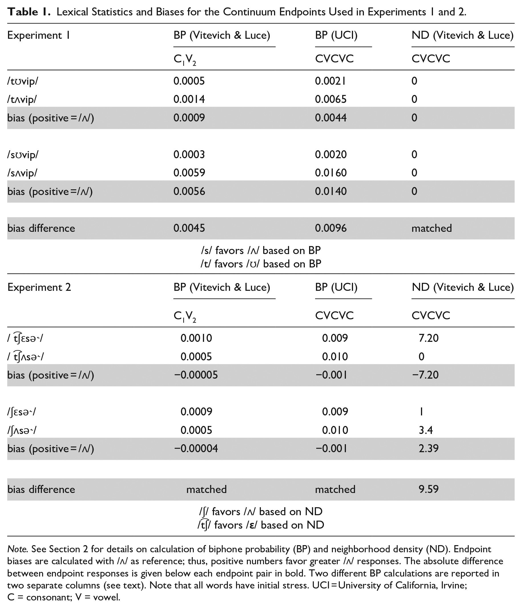
Note. See Section 2 for details on calculation of biphone probability (BP) and neighborhood density (ND). Endpoint biases are calculated with /ʌ/ as reference; thus, positive numbers favor greater /ʌ/ responses. The absolute difference between endpoint responses is given below each endpoint pair in bold. Two different BP calculations are reported in two separate columns (see text). Note that all words have initial stress. UCI = University of California, Irvine; C = consonant; V = vowel.
For BP, the relevant metric is the continuum bias, that is, the BP of one endpoint of the continuum subtracted from the other. These were calculated in Experiment 1 by subtracting the BP for the critical biphone in the /ʊ/ endpoint from the BP in the /ʌ/ endpoint, with a positive value indicating that BP favors /ʌ/. As shown in Table 1, using the Vitevitch & Luce Metrics (KU Phonotactic probability calculator), the C1V2 portion of the /tʊvip/~/tʌvip/ continuum exhibited an /ʌ/ bias (0.0009). The /sʊvip/~/sʌvip/ continuum has an /ʌ/ bias as well (0.0056). When considering the effect of manipulating BP via the initial consonant, the relevant metric is the difference in biases for the two continua. This value (0.0045) predicts the following: the stronger /ʌ/ bias in the /sʊvip/~/sʌvip/ continuum favors perception of /ʌ/ with an initial /s/; the relatively smaller /ʌ/ bias in the /tʊvip/~/tʌvip/ predicts that an initial /t/ should favor perception of /ʊ/ (relative to initial /s/). The metrics computed using the UCI Calculator for the full CVCVC sequence are also consistent with this conclusion: an initial /s/ is predicted to bias listeners toward /ʌ/.
Next consider the stimuli in Experiment 2. The nonwords in Experiment 2 controlled for differences in BP, while varying ND to the largest extent possible (subject to the aforementioned constraints in stimulus selection). The two continua are essentially matched for BP according to both BP computations. Conversely, they vary in ND, for which the biases can be considered in the same way as the BP biases in Experiment 1. /t͡ʃεsə˞/ has a frequency-weighted neighborhood density of 7.2 as compared with zero for the /t͡ʃʌsə˞/ endpoint of the continuum (no phonological neighbors). We indexed the magnitude of this bias by subtracting the frequency-weighted neighborhood density of /t͡ʃεsə˞/ from that of /t͡ʃʌsə˞/. The /t͡ʃεsə˞/~/t͡ʃʌsə˞/ continuum therefore has a neighborhood density bias that is negative, that is, biased toward /ε/. Following Newman et al., listeners should be biased toward a denser-neighborhood nonword when exposed to an ambiguous stimulus. This predicts that ND biases favor perception of /ε/ in this continuum. The ND bias for the /ʃεsə˞/~/ʃʌsə˞/ continuum goes in the opposite direction, whereby the /ʃʌsə˞/ endpoint has greater ND than the /ʃεsə˞/ endpoint, predicting that an initial /ʃ/ should favor /ʌ/ responses.
2.3 Stimuli
For the stimuli in all experiments reported here, we created a vowel quality continuum in which each endpoint was a clear rendition of a particular vowel. The continuum was synthesized in Praat via LPC decomposition and resynthesis of F1, F2, and F3 using a Praat script (Winn, 2016). The stimuli for Experiments 1 and 2 were recorded by a female speaker of American English. The speaker was recorded in a sound-attenuated booth using a Shure SM81 Condenser Handheld Microphone and Pop Filter, with a sampling rate of 44.1 kHz (32 bit).
2.3.1 Experiment 1 stimuli
The stimuli in Experiment 1 were constructed based on the speaker’s natural productions of /sʌvip/ and /sʊvip/. /sʊvip/ served as the base file from which the continuum was created. The frication of the initial /s/ was spliced out of the frame, and the first three formants were varied along a 10-step continuum interpolating in evenly Bark-spaced steps between the formant values for the /ʊ/ base and the speaker’s production of /ʌ/ in /sʌvip/. Higher frequency energy and the pitch contour were preserved during resynthesis such that they matched that of the original /ʊ/ token. The resulting 10-step continuum therefore varied only in the frequencies of the first three formants. The BP-manipulating initial consonant was next spliced preceding the continuum creating 20 unique stimuli (10 continuum steps in each of two frames). The initial /t/ was spliced from the speaker’s production of /tʌvip/, which was chosen in case any traces of the following vowel were present in the production of the stop (though none were perceived). In the case that any biasing information is present in the initial consonant, it would accordingly bias toward /ʌ/, the opposite of the predicted BP effect. The initial /s/ spliced was spliced from the speakers’ production of /sʊvip/ for the same reason.
2.3.2 Experiment 2 stimuli
The procedure for creating stimuli in Experiment 2 was similar to that in Experiment 1. The speaker’s productions of /t͡ʃεsə˞/ and /t͡ʃʌsə˞/ were used. /t͡ʃεsə˞/ served as the base file from which the continuum was created, with the initial consonant spliced out, with the continuum created by Bark-spaced interpolation in F1, F2, and F3 to the values from the /t͡ʃʌsə˞/ endpoint. /ʃ/ was then spliced from a production of /ʃεsə˞/, which was chosen in case any potentially biasing information about the vowel was present in the initial consonant, in which case it would favor /ε/ responses, predicting the opposite of the ND effect. Unlike in Experiment 1, we directly manipulated the initial /ʃ/ to create /t͡ʃ/. The duration of frication is a strong cue for the distinction between these two phonemes, which when manipulated causes perception to shift from one to the other (Howell & Rosen, 1983; Kluender & Walsh, 1992). Kluender and Walsh (1992) show that shorter fricative duration is perceived as /t͡ʃ/, while longer duration is perceived as /ʃ/. The original duration of /ʃ/ was 170 ms in duration, which was reduced to 70 ms, by excising the central 100 ms of fricative noise; this also decreased the amplitude rise time, another cue to the contrast (Howell & Rosen, 1983). The shortened initial fricative was perceived clearly to be /t͡ʃ/, and this manipulation has the advantage of ensuring that the spectral acoustic traits of the consonant preceding the vowel are highly similar, while still conveying a clear distinction between /t͡ʃ/ and /ʃ/.
2.4 Procedure
Data for Experiments 1 and 2 were collected remotely (due to the COVID-19 pandemic). All participants were instructed to take part in the experiment in a quiet space, and to use headphones. The task was a simple two-alternative forced choice (2AFC) task, in which an auditory stimulus was categorized by listeners as one of two nonwords. They were told that they would hear a speaker of English say nonce words, and that their task was simply to select which word they heard. We opted to present only the crucial vowel as a visual choice for participants so that the visual display from trial to trial was the same and there was no orthographic influence in a presentation of the (varying) initial consonant. During a trial, participants were presented visually with two buttons placed on either side of the computer screen, labeled with “OO” and “U” in Experiment 1. Prior to the test trials, participants were instructed that they should select “OO” if they heard the sound /ʊ/, and “U” if they heard the sound /ʌ/. This was conveyed in the task instructions by giving examples of real words that contained these vowels and the same orthographic representation for the vowels (“book”/“buck,” “took”/“tuck”). Participants indicated their response by keypress, where an “f” key-press indicated the button on the left side of the screen and a “j” keypress indicated a letter on the right side of the screen. The side of the screen on which each button appeared was counterbalanced across participants, but for a given participant the side of the screen on which each button appeared was always the same. Participants completed eight practice trials in which they heard each continuum endpoint two times. During test trials, participants heard each unique stimulus 10 times for a total of 200 trials. Stimuli were completely randomized. Testing took about 15 min. The procedure for Experiment 2 was identical to that in Experiment 1, except that “E” and “U” were used as orthographic representations of /ε/ and /ʌ/, respectively.
2.5 Statistical modeling
Categorization results were analyzed using Bayesian mixed-effects logistic regression, with the brms package (Bürkner, 2018) in R with the RStudio environment (RStudio Team, 2020; Posit Team, 2023). All models run in brms here were set to draw 4,000 samples in each of four Markov chains from the distribution of over parameter values, using a no U-turn sampler. Each chain was set to have a burn-in period of 1,000 samples, such that we retained the latter 75% of samples from each chain for inference. In all of the models we report here, we inspected the adequacy of the model fit in examining the R̂ values for each estimate, which serves as a convergence diagnostic in comparing within- and between-chain estimates. R̂ was within 0.01 of the value of 1 in all models reported here, indicating convergence. 1 Models of the categorization data (in this and subsequent experiments) predicted the log odds of selecting a given vowel response as a function of the step of the continuum, the consonantal frame (manipulating BP or ND), and their interaction. In each experiment, the continuum step variable was treated as continuous, and scaled and centered, and the frame variable was contrast coded (described for each experiment below). We additionally included a quadratic term for continuum step in the model, which allows us to model the potentially larger effect of frame in the middle region of the continuum when interacted with the frame variable. Random effects in the model included by-participant intercepts with maximally specified random slopes including both fixed effects and their interaction.
We employed weakly informative normally-distributed priors for both the intercept and for fixed effects: in both cases normal (0,1.5) (in log-odds space). In describing the results, we report the model estimates of effects and their distribution using the p_direction (“probability of direction”) function in the package bayestestR (Makowski et al., 2019). This measure indexes the percentage of the posterior for an effect which shows a given sign, and ranges between 50% and 100%, if 99% of a given posterior is estimated to be positive, this would constitute strong evidence for an effect with that directionality. We would report the above case as pd = 99%. We take pd > 95% to represent robust evidence for an effect. We additionally report the 95% credible intervals (CrI) into which the posterior estimates for an effect fall. This gives an estimate of the breadth of the distribution, and when the interval excludes zero, this can be taken as further evidence for a robust effect. The pd metric and CrI are directly related (both are measures of a posterior distribution’s location in terms of positive/negative estimates). A pd value of 97.5% or greater corresponds to 95% CrI which exclude zero. The advantage of reporting both metrics is that the pd values are more easily interpreted as an index of strength of evidence for effect existence, than the binary assessment of whether or not CrI include the value of zero.
2.6 Participants
In all experiments, we excluded participants who did not respond to the acoustics of the continuum. Employing a similar method as that described in Bushong and Jaeger (2019), we identified these participants by running an individual regression analyses for each participant in brms. In each participants’ individual model, we predicted their categorization responses as a function of continuum step only (with no random effects). A participant who showed no evidence for an effect of continuum step in the model is one who did not shift categorization as a function of changing vowel formants in the experiment. We reasoned that these participants should be excluded from analysis, as they did not show sensitivity to vowel acoustics, suggesting inattention to the task, or a misunderstanding of the task. Sensitivity to the acoustics of the continuum was defined using the pd metric described in Section 2.5. Participants were included when pd > 80. Thus, only participants who did not show any reliable evidence for an effect of vowel acoustics on categorization were excluded. The code implementing this exclusion process is included in full in the supplementary materials for the paper on the OSF (https://osf.io/eba2v/) (as are the sample categorization functions for included and excluded participants).
We recruited 35 participants for Experiment 1 and 34 participants for Experiment 2. In all, 3 participants were excluded from Experiments 1 and 2 were excluded from Experiment 2 by the criterion described above, leaving 32 participants in each experiment. Participants were students at a North American University and received course credit for participation. For all experiments reported here, no participant took part in more than one experiment.
2.7 Results: Experiment 1
The model for Experiment 1 predicted the log odds of an /ʊ/ response (/ʌ/ mapped to 0 and /ʊ/ mapped to 1). The main effect of step was credible, as expected (β = 2.21, CrI = [1.83, 2.60]; pd = 100%), confirming that listeners’ /ʊ/ responses increased along the continuum, as continuum step increased numerically toward the /ʊ/ endpoint. The main effect of consonantal frame, which was coded with /s/ mapped to −0.5, and /t/ mapped to 0.5, was also credible (β = 0.44, CrI = [0.05, 0.84]; pd = 99%). The effect of frame indicates that, consistent with biphone probability effects, participants showed an overall bias to categorize the target as /ʊ/ in the /tV/ frame compared with the /sV/ frame (i.e., more /ʊ/ responses in the /tV/ frame, more /ʌ/ responses in the /sV/ frame). This is shown in Figure 1, where the model fit also indicates a generally larger separation in categorization in the middle region of the continuum. The interaction between consonant frame and the quadratic term for step was found to be robust (pd = 98) in line with this larger separation in the middle of the continuum. The interaction between consonant frame and the linear term was less robust (pd = 93), suggesting that the effect was not particularly stronger at either end of the continuum, though somewhat larger at numerically lower steps (Figure 1).
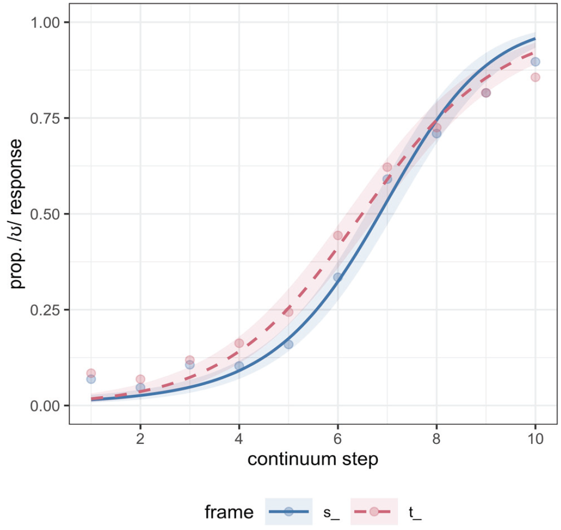
Experiment 1 categorization responses along the continuum (x axis, where Step 1 is the most /ʌ/- like), split by consonant frame. The proportion of /ʊ/ responses is plotted on the y axis. Points are the empirical data and lines are the model fit with 80% credible intervals from the model fit plotted.
The results of Experiment 1 indicate that biphone probability can indeed modulate listeners’ categorization of phonetic continua, as described by Pitt and McQueen (1998). Crucially, these results cannot be attributed to differences in neighborhood densities because we controlled for them during the stimulus selection. In addition, these differences in categorization were restricted to the more ambiguous steps on the continuum, as indicated by the interaction of frame with the quadratic step term, expected if biphone probabilities directly modify input sensory representations (e.g., Massaro, 1989; Massaro & Cowan, 1993). In contrast, effects of decision bias involve vertical shifts in categorization functions, which are not localized to ambiguous stimuli (e.g., Massaro & Cowan, 1993; Norris et al., 2000).
2.8 Results: Experiment 2
Experiment 1 showed a clear effect of biphone probability in phonetic categorization of a nonword continuum, which was independent of neighborhood density. In Experiment 2, we tested if we could obtain evidence for an independent effect of neighborhood density. Results are shown in Figure 2, where “ch” indicates / t͡ʃ/ and “sh” indicates /ʃ/.
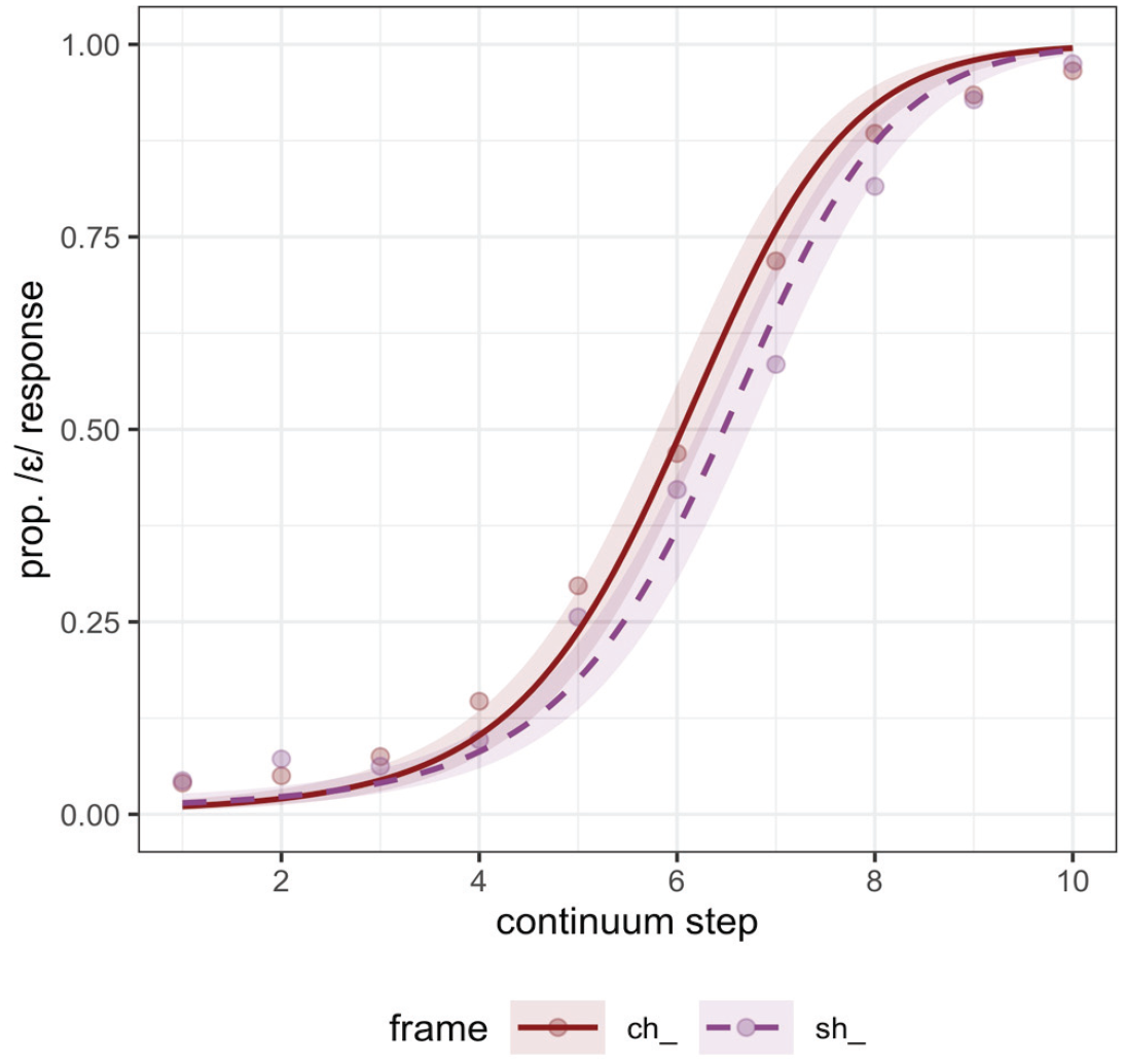
Experiment 2 categorization responses along the continuum (where Step 1 is the most /ʌ/-like), split by consonant frame. The proportion of /ε/ responses is plotted on the y axis.
The model for Experiment 2 predicted the log odds of an /ε/ response (/ʌ/ mapped to 0 and /ε/ mapped to 1). As expected, there was a credible effect of continuum step (β = 3.05, CrI = [2.58, 3.52]; pd = 100%), showing that /ε/ responses increased along the continuum as continuum step increased numerically toward the /ε/ endpoint of the continuum. The main effect of consonantal frame, which was coded with / t͡ʃ/ mapped to −0.5, and /ʃ/ mapped to 0.5, was also credible (β = −0.43, CrI = [−0.76, −0.11]; pd = 99%), showing that, consistent with predicted ND effects, an initial /t͡ʃ/ favors perception of /ε/, with more /ε/ responses in that frame, and /ʃ/ favoring perception of /ʌ/, with fewer /ε/ responses in that frame. There was additionally weaker evidence for a credible interaction between the consonant frame and linear term for continuum step (pd = 94), indicating a larger frame effect at the numerically higher steps of the continuum. Notably though, unlike in Experiment 1, there was no evidence for an interaction with the frame variable and the quadratic term for continuum step (pd = 81), indicating that there was not a larger effect in the middle of the continuum. These results replicate Newman et al.’s findings that neighborhood density affects phonetic categorization, and they preclude a biphone probability difference as a possible confound.
3 Experiments 3 and 4: replicating the effects with highly controlled stimuli
Experiments 1 and 2 have provided us with some first evidence for independent BP and ND effects, showing that each respective influence occurs with the other controlled. In the experiments that follow, we seek to replicate these effects using different frames and continua. In the following experiments we sought to control our materials more tightly, using the same exact acoustic continuum for both BP (Experiment 3) and ND (Experiment 4) manipulations. Converging evidence for these effects across different continua will strengthen the evidence for the existence of independent BP and ND effects.
To this end, we created a continuum from the English vowels /ε/ to /æ/ by manipulating F1, F2, and F3 as in Experiments 1 and 2. This vowel contrast is the one that is tested in all subsequent experiments here. The continuum was presented in one of two CVC frames and listeners were asked to categorize the vowel as /ε/ or /æ/. The two frames in Experiment 3 were: /mεb/~/mæb/ and /mεv/~/mæv/. As with Experiment 1, the consonant frames were selected such that neither endpoint was a word in English, and both coda consonants /b/ and /v/ involved labial constrictions so formant trajectories at the offset of the vowel should be similar, allowing for identical continuum steps to be used with each frame. Table 2 shows the relevant BP and ND statistics for Experiments 3 and 4, with the same layout as Table 1.
Lexical Statistics and Biases for the Continuum Endpoints Used in Experiments 3 and 4.
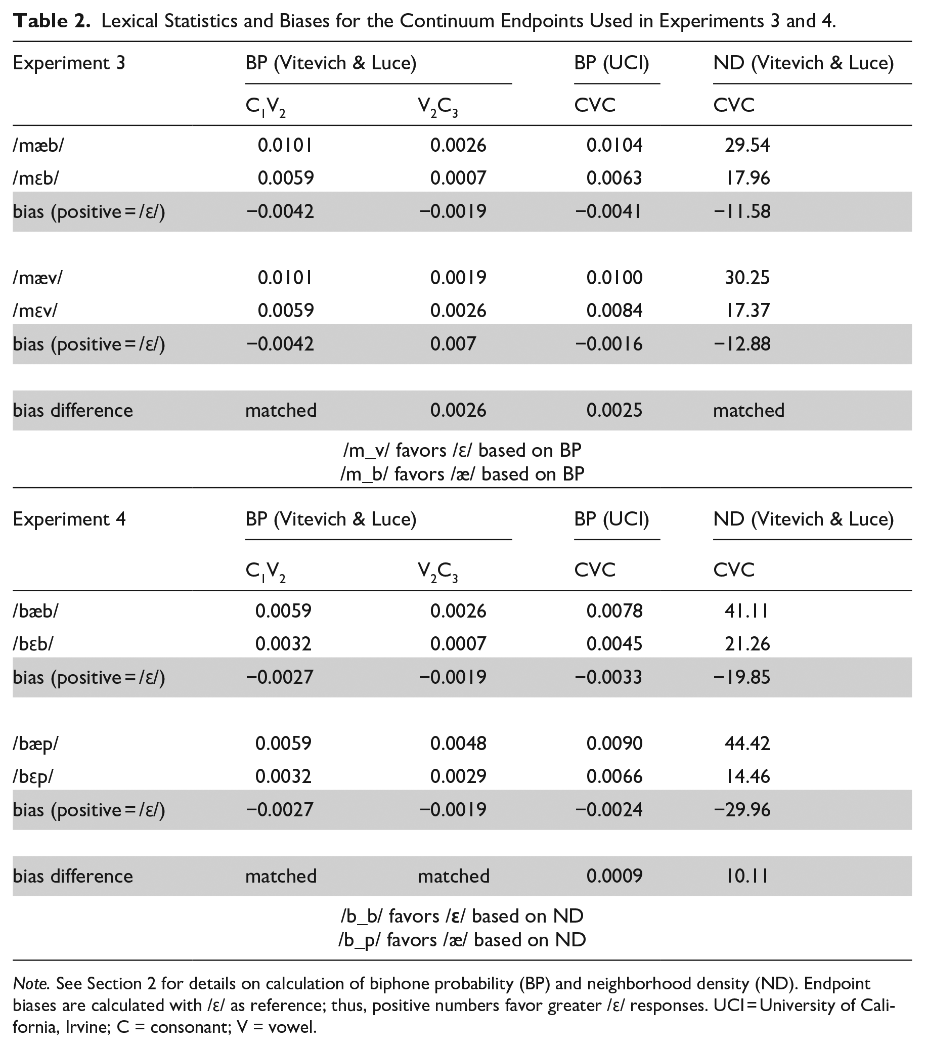
Note. See Section 2 for details on calculation of biphone probability (BP) and neighborhood density (ND). Endpoint biases are calculated with /ɛ/ as reference; thus, positive numbers favor greater /ɛ/ responses. UCI = University of California, Irvine; C = consonant; V = vowel.
3.1 BP and ND metrics in Experiments 3 and 4
First consider neighborhood density for the full CVC sequence of the two continua used in Experiment 3, shown in Table 2: the nonword /mεb/ has a frequency-weighted neighborhood density of 17.96. The other endpoint of the continuum, /mæb/ has a frequency-weighted neighborhood density of 29.54. In this case, a denser neighborhood for /mæb/ would bias listeners to respond /æ/ when exposed to ambiguous items on a /mεb/~/mæb/ continuum. The bias in the /mεb/~/mæb/ continuum is −11.58 (17.96–29.54). The /mεv/~/mæv/ continuum also has a neighborhood density bias for /æ/ of (−12.88). Comparing the biases for the two continua, we see that although both have an /æ/ bias, the /mεv/~/mæv/ continuum has a slightly larger one. This would predict that if listeners are sensitive to neighborhood density alone, they should show increased /æ/ responses to the /mεv/~/mæv/ continuum compared with /mεb/~/mæb/ continuum. However, it should be noted that the difference in ND bias across continua here is much smaller than reported for the continua used by Newman et al. (1997). For example, their velar place of articulation continuum showed a bias difference of 14.5, and their labial place of articulation continuum showed a bias difference of 8.7, as compared with our difference of 1.3, suggesting that the influence of ND here may be minimal.
Using the Vitevitch & Luce Metrics (KU Phonotactic probability calculator), the V2 C3 portion of the /mεb/~/mæb/ continuum exhibited an /æ/ bias (−0.0019), while the V2C3 portion of the /mεv/~/mæv/ continuum exhibited an /ε/ bias (0.0007). This differential predicts that a coda /b/ should bias listeners toward /æ/ responses, such that they prefer a relatively higher probability sequence /mæb/ (as compared with /mεb/), and vice versa for coda /v/. The metrics computed using the UCI Calculator for the full CVC sequence are also consistent with this conclusion: a coda /v/ biases listeners toward /ε/ in Experiment 3. If listeners are sensitive to biphone probability information, they should thus show increased /ε/ responses for the /mεv/~/mæv/ continuum compared with the /mεb/~/mæb/ continuum, with coda /v/ biasing toward /ε/. Note that the bias based on biphone probability is in the opposite direction than the bias predicted by neighborhood density, making this a fairly conservative test for biphone probability effects (though density biases are minimally different).
In Experiment 4, two new continua were created: /bεp/~/bæp/ and /bεb/~/bæb/. V2C3 biphone probability was matched for these two pairs (see Table 2), such that they both exhibited an equal /ε/ bias (−0.0019). Unlike Experiment 3, however, the neighborhood density bias for these continua differed: both exhibited an /æ/ bias, with the bias for the /bεp/~/bæp/ continuum (−29.35) stronger than that for the /bεb/~/bæb/ continuum (−19.85). A denser neighborhood should bias listeners toward /æ/ responses, predicting more /æ/ responses for the /bεp/~/bæp/ continuum. Such a finding could not be explained by differences in biphone probability, which are matched (see Table 2). The empirical prediction is thus that a coda /b/ frame should show increased /ε/ responses (decreased /æ/ responses), as ND differences favor /æ/ more strongly in the frame with coda /p/. Here we note that the UCI phonotactic probability calculator differs slightly from the KU phonotactic probability calculator, in showing a small bias difference with coda /p/ slightly favoring /ε/, the opposite of the predicted ND effect.
The two frames used in Experiment 4, /b/ and /p/, differ in voicing of the coda consonants. We know from previous research that consonant voicing has an effect on vowel formants, such that the presence of voicing generally lowers F1 (e.g., Hillenbrand et al., 2001). Thus, listeners might expect F1 lowering (or, vowel raising in the vowel space given that higher vowels have lower F1) with a coda /b/. If this is the case, lower (more /ε/-like) F1 values should be categorized as /æ/ when /b/ follows (as compared with /p/), thereby increasing /æ/ responses in the context of a coda /b/. This possible voicing effect runs counter to the predicted effect of neighborhood density making this a conservative test for the neighborhood density effect.
3.2 Materials
Stimuli for Experiments 3–6 were created by resynthesizing the speech of an adult male speaker of American English. The stimuli were first recorded at 44.1 kHz (32 bit) in a sound-attenuated booth, using an SM10A ShureTM microphone and headset (note that the speaker for these stimuli is different than the speaker for Experiments 1 and 2 due to the interval of time between them).
The creation of the stimuli followed the same approach as in Experiments 1 and 2. The starting point for the creation of stimuli in Experiment 3 was the speaker’s natural production of two CVC nonwords: /mεv/ and /mæv/. The vocalic portion of both of these nonwords was excised from the CVC frame. Resynthesis used /ε/ as a base and interpolated F1, F2, and F3 in 12 even, Bark-spaced steps to their respective values for the /æ/ token. The higher frequency energy and pitch contour were preserved during resynthesis such that they matched that of the original /ε/ token. The resulting 12-step continuum therefore varied only in the frequencies of the first three formants. The onset /m/ from the original production of /mεv/ was then respliced onto each continuum. The coda /b/ and /v/ were cross-spliced from productions of /mεb/ and /mæv/, respectively. As with Experiments 1 and 2, this was done to remove any possible acoustic traces of co-articulatory information from the preceding vowel cuing these consonants; though it is unlikely that the cross-spliced stop closure/release and fricative noise contained cues to identify the original preceding vowel. Specifically, given that we predicted a following /v/ should bias listeners toward /ε/ categorization, as outlined above, the cross-spliced /v/ came from a post-/æ/ context, ensuring any possible acoustic information from the preceding vowel would predict the opposite adjustment in categorization. For the same reason /b/ was cross-spliced from a post-/ε/ context. These manipulations created 24 unique stimuli (12 continuum steps × 2 consonant frames). We note here that both coda consonants /b/ and /v/ are phonologically voiced (and realized as voiced in the stimuli); this is pertinent given that voicing has been shown to influence vowel formants in speech production as noted above (a point we return to in discussing Experiment 4). Both consonants are in similar places of articulation (labial and labio-dental) such that we would not expect a place of articulation effects on vowel formants (Hillenbrand et al., 2001).
We used the same vowel continuum in Experiments 3 and 4, however, we presented them in different frames. The new frame consonants were cross-spliced from the same speakers’ productions. The initial /b/ was cross-spliced from a production of /bεb/. The coda /b/ was cross-spliced from a production of /bæb/, and the coda /p/ was cross-spliced from a production of /bεp/. As with Experiment 3, this method of cross splicing was chosen to remove any possible acoustic traces of the preceding vowel on cross-spliced coda consonants. Specifically, because we predicted that the /bæp/~/bεp/ continuum should bias categorization toward /æ/ (as compared with /bæb/~/bεb/), the coda /p/ was cross-spliced from an original /εp/ sequence. Likewise, the coda /b/ was cross-spliced from an original /æb/ sequence. Because the consonants used in Experiment 3 also involved labial constrictions, formant transitions at the onset and offset of the vowel continuum were judged to sound natural in these new frames.
3.3 Participants in Experiments 3 and 4
For both Experiments 3 and 4, 35 (different) self-identified native speakers of American English with normal hearing were recruited. In both experiments, four participants were excluded by the process described in Section 2.4, retaining 31 for analysis. Participants were students at a North American University and received course credit for participation.
3.4 Procedure
These experiments were completed in person, unlike Experiments 1 and 2. Participants completed the task seated in front of a desktop computer, in a sound-attenuated booth in the lab. Stimuli were presented binaurally via a 3MTM PeltorTM listen-only headset. They were told that they would hear a speaker of English say nonce words, and that their task was simply to select which word they heard. During a trial, participants were presented visually with two letters placed on either side of the computer screen: “E” and “A.” Prior to the trials beginning, participants were instructed that they should select “E” if they heard the sound /ε/, and “A” if they heard the sound /æ/. As with Experiments 1 and 2, this was conveyed by giving examples of real words that rhymed with the nonword continuum endpoints in the task instructions. Participants indicated their response by keypress, where an “f” key-press indicated the letter on the left side of the screen and a “j” keypress indicated a letter on the right side of the screen. The side of the screen on which each letter appeared was counterbalanced across participants. Participants completed 8 practice trials in which they heard each continuum endpoint in each CVC frame two times. During test trials, participants heard each unique stimulus 8 times for a total of 192 trials. Stimuli were completely randomized. Testing took about 15 min. The procedure for Experiment 4 was identical to that in Experiment 3, and took about 15 min.
3.5 Results: Experiment 3
In the model for Experiment 3, the main effect of step was credible as expected (β = 2.80, CrI = [2.23, 3.37]; pd = 100%), confirming that listeners’ /ε/ responses increased along the continuum. The main effect of consonantal frame, with /mVb/ mapped to −0.5, and /mVv/ mapped to 0.5, was also credible (β = 0.33, CrI = [0.07, 0.59]; pd = 99%). The effect of frame indicates that, consistent with biphone probability effects, participants showed an overall bias to categorize the target as /ε/ in the /mVv/ frame compared with the /mVb/ frame. This is shown in Figure 3, wherein the model fit also indicates a generally larger separation in categorization in the middle region of the continuum. The interaction between consonant frame and the quadratic term for step was found to be robust (pd = 96), in line with this larger separation in the middle of the continuum, as was also found for the BP effect in Experiment 1. The interaction between consonant frame and the linear term was not robust (pd = 80), suggesting the effect was not larger at either end of the continuum.
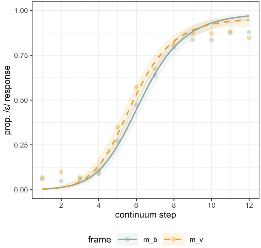
Experiment 3 categorization responses along the continuum (x axis, where Step 1 is the most /æ/- like), split by consonant frame. The proportion of /ɛ/ responses is plotted on the y axis.
The results of Experiment 3, replicate those in Experiment 1, and provide further confirmation that BP influences phonetic categorization. In Experiment 5, we directly test the time course of the biphone probability effect. We can further compare the effect we see here to two previous studies in which biphone probability effects were manipulated.
To compare BP differences from our Experiments 1 and 3 with those in Pitt and McQueen (1998), we computed BP metrics for the set of stimuli which differed on BP (their Experiment 4). According to the KU phonotactic probability calculator, the bias difference in Pitt & McQueen’s experiment was 0.0008, compared with 0.0045 (Experiment 1) and 0.0026 (Experiment 3) in our case. This suggests that listeners are sensitive to even smaller bias differences than the one we tested here. We can also make a comparison to the stimuli used by Kingston et al. (2016), described in detail in Section 4 below. The BP bias in their Experiment 4 is comparable to the BP bias in Experiment 3 based on the KU phonotactic metric (0.0024 compared with our 0.0026), though their effect size, comparable to ours in being modeled via logistic regression, is much larger in magnitude. This is likely due to the denser sampling of the ambiguous regions of the acoustic continuum in Kingston et al. (2016).
3.6 Results: Experiment 4
The model specifications and model fitting procedure were identical to that in Experiment 3. The results are plotted in Figure 4. In contrast coding consonant frame, /bVp/ was mapped to −0.5 and /bVb/ was mapped to 0.5. As in Experiment 3, the expected main effect of step was credible (β = 3.92, CrI = [3.36, 4.50]; pd = 100%). The main effect of consonant frame was also present, though smaller in magnitude with 95% CrI only narrowly including zero (β = 0.24, CrI = [−0.03, 0.53]; pd = 96%). In Figure 4, we can see the effect of consonant frame: consistent with predicted neighborhood density effects, listeners showed increased /ε/ responses with the /bVb/ frame, shifting categorization in accordance with neighborhood density. The interactions between continuum step were not credible either for the linear (pd = 86) or quadratic term (pd = 64). The very weak evidence for an interaction with the linear term derives from the slightly larger separation between frames at higher continuum steps, which would be consistent with a decision bias.
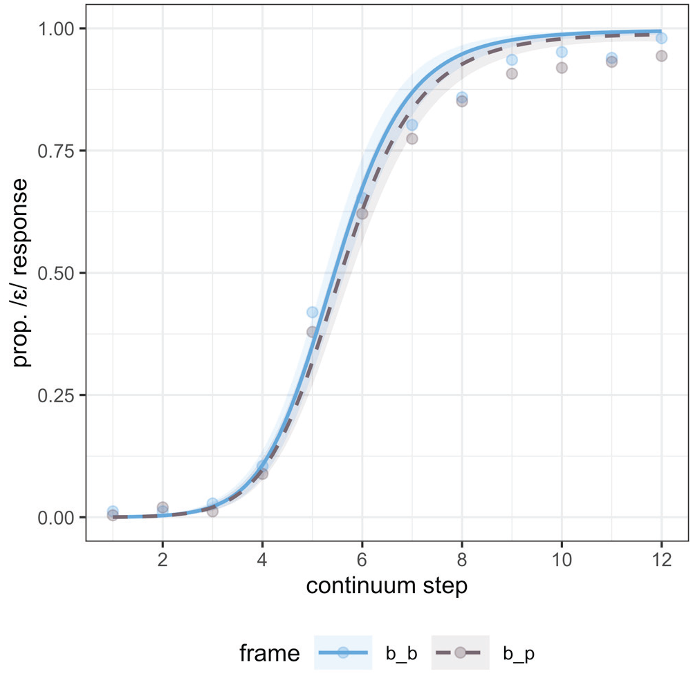
Experiment 4 categorization responses along the continuum, split by consonant frame.
Experiments 2 and 4 together provide fairly convincing evidence for the existence of independent ND effects, though the strength of evidence for an effect is weaker in Experiment 4 and the effect is smaller, though ND differences are similar. Several possible explanations for this difference can be considered. First, as described above, a possible competing effect exists in Experiment 4: the influence of coda voicing differences in the ND manipulating consonant. It is possible that this countervailing influence weakened the ND effect. Second, the location of the ND-manipulating material was different across experiments. In Experiment 2, the initial consonant in a CVCV word varied to manipulate ND, while in Experiment 4, the final consonant in a CVC word varied. As discussed above, ND effects are hypothesized to be post-lexical and based on feedback, occurring later in processing, as shown in part by Newman et al.’s (1997) finding that their ND effects were larger at slower reaction times. The additional time that listeners have to accumulate unfolding ND information in Experiment 2 (as compared with Experiment 4) may have led to stronger ND effects. Especially, if listeners categorize the stimuli in Experiment 4 quickly, it is possible that this decreased the strength of the ND effect. The explanations proposed here are somewhat speculative, however, the lack of an interaction between the quadratic term for continuum step and the frame variable is consistent with a later-stage decision bias effect for ND. This notably contrasts with the presence of this interaction for both BP effects in Experiments 1 and 3.
4 Experiment 5: time course of biphone probability and neighborhood density effects
Taking Experiments 1–4 together, we have evidence for the independent influence of both biphone probability and neighborhood density as indexed by listeners’ categorization responses. However, categorization performance only provides a measure of the endpoint of the speech recognition process. To obtain precise timing information about when BP and ND affect recognition, we need evidence from online tasks. Previous research, outlined below, offers some relevant time course comparisons.
Using brain imaging, Pylkkänen et al. (2002) provide some evidence that biphone probability effects are consistently observed between 300 and 400 ms post-stimulus onset. In an MEG experiment, they administered a lexical decision task to listeners who were presented with CVC sequences that were either high probability and high density or low probability and low density. They investigated an MEG response component—M350—which peaks between 300 and 400 ms post-stimulus onset. Because the M350 was facilitated in response to the manipulated probability, and not inhibited as expected for a density manipulation, Pylkkänen et al. argue that the M350 is sensitive to biphone probability. They did not find a clear correlate of the density effect in later MEG components. Thus, the MEG results present an estimate of the timeline for probability effects, and indirect support that this may be different from the effect of neighborhood density (see also Pylkkänen & Marantz, 2003).
More recently, Kingston and colleagues (Kingston et al., 2016) reported on two experiments where they evaluated the time course of lexical effects on phonetic processing. In Kingston et al.’s experiments, listeners were asked to categorize a word to nonword phonetic continuum. They reasoned that if lexical effects are driven by feedback, they should be delayed as demonstrated in TRACE simulations (McClelland & Elman, 1986). However, a rapid use of lexical information in categorization would constitute evidence against feedback, and be more consistent with a feed-forward account. Based on results from two eye-tracking experiments, Kingston et al. claim that lexical effects influence phonetic processing between 300 and 400 ms after stimulus onset, and thus are too early to be consistent with feedback.
A closer look at Kingston et al.’s experiments, however, offers an alternative explanation for their findings. First, in Kingston et al.’s Experiment 4a—the lexical effect is confounded with a biphone probability effect. In this experiment, listeners were presented with a continuum ranging between the vowels /ε/ and /ʌ/ in a CVC(C) frame; whether the endpoint was a word or nonword was determined by the final consonant. The continuum was placed in one of four frames: (1) /b _ ŋk/ forming the word “bunk” with /ʌ/, (2) /d _ ŋk/ forming the word “dunk” with /ʌ/, (3) /b _ ʃ/ and (4) /d _ ʃ/ (both resulting in nonwords). The initial consonant was varied to manipulate spectral context, and will not be discussed here; its inclusion does not alter the conclusions based on biphone probability differences discussed below. Because a coda /ŋk/ creates words with the vowel /ʌ/, but not /ε/, Kingston et al. predicted that /ŋk/ should increase looks to an orthographic representation of /ʌ/ (“U”), as compared with a following /ʃ/. This is what the authors found, with the influence of the coda consonant(s) emerging within 300–400 ms of stimulus onset.
A different interpretation of these finding emerges if we compare the biphone probabilities for the vowel and following consonant sequence. In the /ʃ/ context, the biphone probabilities are essentially matched with a very slight /ʌ/ bias: 0.0002 for /Cεʃ/ and 0.0004 /Cʌʃ/. However, the biphone probability for the vowel and following consonant /ŋ/, reveals an asymmetry: a following /ŋ/ engenders a stronger /ʌ/ bias: 0.0003 for /Cεŋ/ and 0.0027 for /Cʌŋ/. The magnitude of this /ʌ/ bias is comparable to our own biphone probability manipulation in Experiment 3. Thus, an alternate explanation for Kingston et al.’s results is that the time course from Experiment 4a reflects a difference in biphone probability between the sequences, and therefore, like in Pylkkänen et al.’s MEG experiment, is observed between 300 and 400 ms post-stimulus onset.
In the other eye-tracking experiment reported by Kingston et al. (Experiment 3a), listeners categorized a continuum of fricative noise that ranged from /s/ to /f/. The continuum was followed by one of three frames: (1) /_ aɪl /, creating a word with /f/ “file,” but not with /s/, (2) /_ aɪd /, creating a word with /s/ “side,” but not with /f/, and (3) control frame /_ aɪm / for which both continuum endpoints were nonwords. The online effect was significant only in the /_ aɪl / frame, with increased looks to a visual “F” target on the screen, in comparison to the control frame. This effect cannot be explained by biphone probability differences; the summed biphone probability of “file” (0.0043) is lower than that of “sile” (0.0058). However, there was no significant difference in looks between the /_ aɪm / frame and the control frame /_ aɪd /, where we would expect to see more looks to a visual “S” target when the lexical context “side” reinforces /s/. This asymmetry in online processing between the two experimental frames makes it difficult to interpret the results from Kingston et al.’s Experiment 3a.
In Experiment 5, we used Kingston et al.’s experimental design with the stimuli used in Experiments 3 and 4, where the effects of biphone probability and neighborhood density were orthogonally manipulated. Specifically, we were interested in how these effects unfold online using a visual world eye-tracking task. Combining categorization with eye-tracking data allowed us to investigate the online integration of information as speech unfolds (unlike reaction times), as discussed in Norris et al. (2000). The eye-movement response to the vowel spectra served as our baseline, because it indexes a (rapid) response to the signal. Given the independence of biphone probability and neighborhood density effects documented in Experiments 1 and 2, respectively, we expected to see an independent influence of each variable in the online task as well. If biphone probability affects the sensory activation of phones, we expected them to emerge soon after the spectral response (once listeners have heard the coda consonant), about 300–400 ms post-stimulus onset consistent with Pylkkänen et al. (2002). Of crucial interest was the relative timing of each effect. If neighborhood density effects originate from a feedback loop between the lexicon and prelexical information, because feedback takes time as modeled in TRACE simulations (McClelland & Elman, 1986), the influence of ND should be delayed in comparison to a spectral response. Recall that Newman et al. (1997) also reported reliable ND effects only at slow and intermediate reaction times, suggesting a later influence in processing.
4.1 Materials
The materials used in Experiment 5 were a subset of those used in Experiments 3 and 4. To present listeners with relatively ambiguous stimulus tokens (following, for example, Mitterer & Reinisch, 2013; Reinisch & Sjerps, 2013), we presented listeners with the most ambiguous region of each continuum. This was identified as the 4-step window centered around the 50% crossover points in the interpolated categorization functions derived from Experiments 3 and 4. In both experiments, this method selected Steps 4 through 7. Participants heard all four continua (/mVb/, /mVv/, /bVb/, /bVp/) at these four steps. There were thus 16 unique stimuli used in Experiment 5 (4 continuum steps × 4 consonant frames).
4.2 Participants
Sixty-eight self-identified native speakers of American English with normal or corrected to normal vision participated in Experiment 3. We subsequently excluded three participants whose gaze data was not recorded consistently due to technical issues. Eight additional participants were excluded because their categorization did not differ based on the acoustics of the continuum as described in Section 2.6, retaining 57 for analysis. Participants were students at a North American University and received course credit for participation.
4.3 Procedure
In Experiment 5, we used a visual world eye-tracking task, with a similar design to that used by Kingston et al. (2016). Participants were seated in front of an arm-mounted SR Eyelink 1000 (SR Research, Mississauga, Canada), which was set to track the left eye remotely, at a sampling rate of 500 Hz, and at a distance of approximately 550 mm. The visual display was presented to participants on a 1,920 × 1,080 ASUS HDMI monitor. Participants were tested in a sound-attenuated room in the lab. Participants’ gaze was calibrated using a 5-point calibration procedure at the start of each experiment.
During an experimental trial, participants were presented with orthographic E and A on the target screen (Kingston et al., 2016) and were instructed to click on the letter corresponding to sound they heard. As in Experiments 1 and 2, examples of real English words that rhymed with the nonwords were given to convey the intended letter-to-sound mapping. Participants’ eye movements were monitored while they performed the task. The orthographic targets were arranged vertically in the visual display, with each letter centered horizontally, and positioned 270 pixels above and below the midpoint of the display. Each letter was presented in 60pt black Arial font. The location of each letter was counterbalanced across participants. Each trial began with the appearance of a black fixation cross in the center of the visual display (60 px by 60 px). Following Kingston et al. (2016), stimulus onset was look-contingent, such that the audio stimulus played only after a look was registered on the fixation cross. Eye-movements were recorded from the first appearance of the fixation cross until a click response was registered by participants. After a click response was provided, the location of the mouse cursor was re-centered on the screen. Each trial was separated by a 1-s interval.
During the experiment, participants heard 8 repetitions of the 16 unique stimuli in a random order, for a total of 128 trials. Participants additionally completed 8 training trials prior to test trials in which they heard Steps 4 and 7 for each frame, to give them practice with the experimental paradigm. The experiment took approximately 20 min to complete.
4.4 Analysis
We report several analyses of the data collected in Experiment 5. We analyzed listeners’ click responses, using a Bayesian mixed-effects model to model the log odds of selecting an /ε/ response as a function of frame (/mVb/, /mVv/, /bVb/, /bVp/), as in Experiments 1-4. The model was fit with the same fixed effects and random effect structure as previous models.
We additionally carried out two complementary eye-tracking analyses. For both, the analysis window was 0–1,200 ms after the onset of the target vowel; listeners typically made a categorization click response within this time period after which there was a substantial drop in recorded eye movements.
First, following Kingston et al. (2016), we report on an analysis of the likelihood of initiating a look to a given target (a saccade) at a given time point in a moving window. This analysis method differs from a more traditional moving window analysis in which the presence of, or proportion of, fixations to a given target (or a transformation of these data) are modeled over a moving window. In the saccadic analysis, only the initiation of a fixation is modeled, that is, whether or not in a given time bin a saccade to the target occurs. As shown by Kingston et al., this metric can diverge from the more traditional analysis, especially with respect to when an effect ends, or diminishes in magnitude. For example, if a fixation is initiated to a given target at 200 ms from target onset and persists for 1 s (see e.g., Staub et al., 2012 for data on the duration of fixations), the traditional analysis will model the fixation as occurring from 200 ms onwards, with its presence in subsequent time bins resulting from its initiation at 200 ms. In contrast, the saccadic analysis will only record the first time-bin at which the fixation was initiated (200 ms). Kingston et al. suggest that this analysis provides a clearer picture of when precisely a given stimuli property impacts eye movements by excluding carry-over effects from continued fixation to a target.
Following Kingston et al., we binned the data into 100-ms intervals, and coded for each time bin the presence/absence of an initiated fixation as a binary variable (1 = initiation of a fixation, 0 = no initiation). For a given bin, we also excluded any fixations to a target following an earlier fixation to the same target in the trial. In other words, if a participant initiated a fixation to a target between 200 and 300 ms, then looked away from the target, then initiated another fixation to the same target at 700–800 ms, only the former of these was counted. Following Kingston et al., we modeled looks to just one target, in our case the /ε/ (orthographic “E”) target. In each 100-ms time bin, a logistic mixed effects regression was run, again using brms, fit with weak normal priors. In each binned regression, the dependent measure was predicted as a function of continuum step (scaled), and frame, which in this case we contrast coded. We subsequently extracted two estimates of pairwise frame differences of interest, using emmeans (Lenth, 2020). These were: /mVb/ versus /mVv/ (indexing the BP effect), and /bVb/ versus /bVp/ (indexing the ND effect). The estimate and distribution for each marginal comparison was then computed, in addition to the effect of continuum step. We note here that we carried out a more traditional moving window analysis as well, modeling listeners Elog-transformed fixation preference (described below) over 100-ms time bins. The code and model results for this additional analysis are included in full in the open access repository (https://osf.io/eba2v/).
As described above, in the saccadic analysis, looks to target in each bin are treated as independent. However, looking behavior is correlated across adjacent time bins (especially in fixation-based analyses), which is sometimes offered as a critique of moving window analyses. We accordingly report a complementary time-series analyses. This additional analysis was carried out using a Generalized Additive Mixed Model (GAMM), which offers a powerful tool for analyzing time-series data from visual world experiments (Nixon et al., 2016; Steffman, 2021; Zahner et al., 2019). GAMMs have recently been advocated for use in modeling eye-movement data, as they (1) easily fit nonlinear trajectory shapes and (2) provide for an intuitive assessment of when eye-tracking trajectories diverge (see Zahner et al., 2019 for similar discussion advocating for GAMMs). The dependent variable for the GAMM analysis was a “preference” measure computed as listeners’ log-transformed fixations on /ε/ subtracted from their log-transformed fixations on /æ/ (see e.g., Reinisch & Sjerps, 2013). Measures were transformed using the empirical logit (Elog) transformation, as described in Barr (2008). The GAMM model was implemented with the mgcv and itsadug packages in R (van Rij et al., 2020; Wood, 2011). We implemented an AR1 error model, following procedures described in Sóskuthy (2017), which reduces residual autocorrelation common in time-series data (see open access model code for implementation). The numerical model output is fairly uninformative for understanding the timing questions asked here (Wood, 2011; Zahner et al., 2019), as such the model summary is available in the scripts included on the open access repository, and we rely on visual inspection of the model fit in what follows. In the GAMM analysis the fixation data was binned in 20-ms intervals (as in Steffman, 2021; Zahner et al., 2019) and thus provides a more fine-grained comparison of timing. To model the relationship between continuum step (with four levels) and consonant frame (with four levels), we created a combined variable of each frame and step combination, with 16 levels in total (e.g., a level for /mVb/ at step 4, a level for /mVv/ at step 4, and so on). Modeling these frame/step combinations as separate trajectories allows us to capture nonlinear differences based on both continuum step and frame. By-participant random smooths over time (factor smooths), as well as factor smooths by the combined frame/step variable, analogous to by-participant intercepts and slopes in mixed models were included (see e.g., Sóskuthy, 2021). For both of the random effect (factor smooth) terms, the m parameter was set to 1 (Baayen et al., 2018). In another version of the model, included in the supplementary materials, we treated continuum step as a continuous parameter and modeled the interaction between step and frame using a tensor production interaction term (cf. Nixon et al., 2016). This alternative model structure led us to the same conclusions about the data.
4.5 Results and discussion
4.5.1 Click responses
Overall, in Experiment 5, the continuum steps we used (4–7) were perceived as more /æ/-like as evidenced by the credibly negative intercept estimate for the reference level which was set to be /mVb/ (β = −0.37, CrI = [−0.65, −0.10]; pd = 100%). This /æ/ bias was stronger than in Experiments 3 and 4, despite selecting the most ambiguous regions based on 50% crossover points in the categorization functions in those same experiments. We can only conclude that listeners recalibrated categorization because of the absence of steps from the endpoints of the continua. Continuum step showed a credible effect, as listeners increased /ε/-responses (β = 1.48, CrI = [1.23, 1.74]; pd = 100%) progressively from Step 4 toward Step 7 where formants were more /ε/-like.
The first comparison of interest was between the frames manipulating biphone probability: /mVb/ versus /mVv/; with /mVb/, as the reference level in the model, the estimate for the /mVv/ frame was credibly positive (β = 0.47, CrI = [−0.01, 0.89]; pd = 97%), replicating the observed difference between these two frames in Experiment 3. There was also evidence for an interaction between continuum step and the /mVv/ frame: (β = 0.29, CrI = [0.02, 0.57]; pd = 98%), showing that the effect of biphone probability was larger at higher continuum steps, as is visible in Figure 5. None of the other interactions between either linear or quadratic step terms and consonant frame were credible.
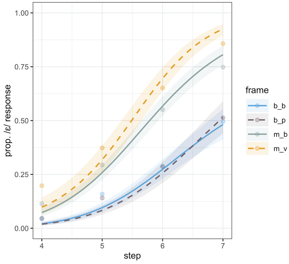
Experiment 5 categorization (click) responses along the continuum, split by consonant frame.
The model estimates showed further that both /bVb/ and /bVp/ frames evidenced credibly decreased /ε/ responses relative to the /mVb/ (/bVb/: β = −1.20, CrI = [−1.59, −0.81]; pd = 100%; /bVp/: β = −1.34, CrI = [−1.76, −0.92]; pd = 100%). This difference in /æ/ responses between the /m/- vs /b/-initial frames was even larger than the biphone probability effect across the /m/-initial frames. Pairwise comparisons between /mVv/ and both /b/-initial frames were examined using emmeans (Lenth, 2020), and as expected based on Figure 5, were each credibly different from one another.
Before we turn to the comparison between /b/-initial frames, let us consider the difference we see here based on initial consonant. This effect emerged in Experiment 5, because we used a within-subject design in contrast to the between-subjects design in Experiments 3 and 4 where the effects of the /m/-initial and /b/-initial frames were investigated separately. We can rule out that this effect was driven by the differences in biphone probabilities of the /m/-initial and /b/-initial frames. From Table 2 (using the Vitevitch & Luce metrics) we see that the biphone sequence /mV/ has a stronger /æ/ bias (−0.0042) compared with /bV/ (−0.0027); this difference in biphone probability would predict the opposite of the effect observed here. Even considering the summed biphone probability of the whole CVC sequence, we see the following gradation in the strength of /æ/ biases, from largest to smallest: /mVb/ (−0.0061) > /bVp/ and /bVb/ (−0.0046) > /mVv/ (−0.0035). This too cannot explain the difference we see between /m/- and /b/-initial frames, because based on this rank ordering the most /æ/ responses are expected for /mVb/, which is clearly not the case.
The direction of difference in /ε/ responses between the /m/- and /b/-initial frames is more consistent with a difference in neighborhood density, with the latter having a stronger /æ/ bias (Table 2). However, there is also reason to be skeptical that neighborhood density differences are driving the difference between /m/- and /b/-initial frames. The difference in neighborhood density between the two /b/-initial frames was at least as large, if not larger in magnitude than the neighborhood density difference between the /m/- and the /b/-initial frames. Yet, the effect between /m/- and /b/-initial frames was credible, whereas the neighborhood density effect indexed by the difference between the two /b/-initial frames was not (reported below).
Instead, we speculate that by introducing different initial consonants in our frames, we may have introduced a new variable that influenced listeners’ perception of the target vowel. A change in initial-consonant from /b/ to /m/ is a switch between an oral and a nasal onset. Although our vowel did not vary in terms of nasality across frames (being originally produced in /m/ initial frames), listeners’ perception of F1 and/or F2 is likely to have been modulated because they were compensating for the typical coarticulatory effects of nasals on vowel formants. Nasalization of vowels adjacent to nasal consonants is well-attested in American English (e.g., Chen et al., 2007; Cohn, 1990; Maeda, 1993). Nasalization typically lowers perceived F1 for low vowels (Diehl et al., 1990), directly impacting listeners’ perception of vowel height adjacent to nasal consonants (Beddor, 1993; Ohala et al., 1986; Wright, 1980). Ohala et al. (1986) present a test case that offers a close comparison to the present stimuli. They found that when a vowel on an /ε/ ~ /æ/ continuum was adjacent to a nasal consonant, but had only very weak nasalization (comparable to the present stimuli where vowels were originally produced in /m/-initial carryover contexts), listeners “overcompensated” for the expected effect of vowel nasalization. An adjacent nasal consonant accordingly led to decreased /æ/ responses, that is, perception of a higher vowel, /ε/. Thus, it is quite likely that the difference between /m/- and /b/-initial frames is due to the listener’s compensation for the nasal context, and not attributable to either biphone probability or neighborhood density differences. We addressed this issue directly in Experiment 6.
The second comparison of interest was between the frames manipulating neighborhood density: /bVb/ versus /bVp/, also extracted using emmeans. Unlike in Experiment 4, there was not evidence for a difference between these two frames used to manipulate neighborhood density (β = 0.14, CrI = [−0.25, 0.54], pd = 76). As we can see from Figure 5, these frames did not induce any reliable shift in categorization. Thus, we did not replicate the neighborhood density effect observed in Experiment 4. Perhaps including more ambiguous steps (e.g., 4 through 9) instead of just the ones around the 50% cross-over points may have allowed ND effects to emerge in Experiment 3. We return to this point in discussing the eye-movement data below.
4.5.2 Eye-movement data
In Figure 6, we plot listeners’ proportion of looks to /ε/ over time (not the log transformed preference measure used in modeling) for ease of visual inspection. In this figure the time course of looks to /ε/, split by consonant frame (a), continuum step (b), and frame faceted by step (c) are presented. First, confirming what we saw in the categorization responses, the eye-movement data show a bias toward /æ/, that is, listeners’ fixations to /ε/ are overall fairly low. Qualitatively, we can note that the frame effects shown in Figure 6(a) mirror the categorization responses described in Section 4.5.1: there is a clear separation between the BP-manipulating frames, with /mVv/ favoring looks to /ε/, in contrast to the ND-manipulating frames, which are generally overlapping. As with the categorization results, we additionally see a robust effect of initial consonant, with /m/-initial frames favoring looks to /ε/.
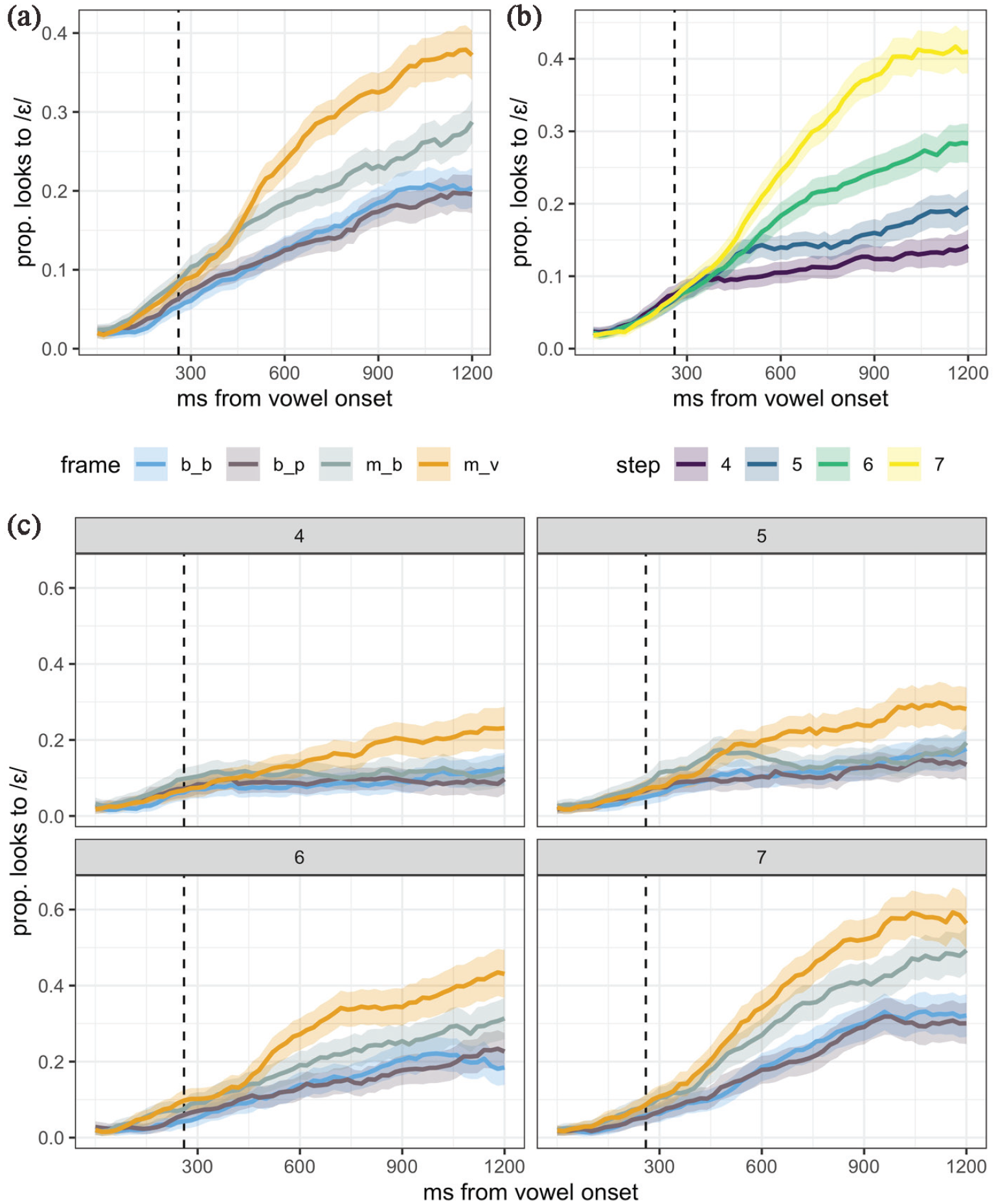
Experiment 5 eye-movement data, split by (a) consonant frame, (b) continuum step, and (c) frame and continuum step. The proportion of looks to /ɛ/ over time is plotted, with 95% confidence intervals computed from the raw data. The dashed vertical line indicates the vowel offset (260 ms).
In panel B, we can see that continuum step exerted an expected influence in online processing: higher values (more /ε/-like steps) favor looks to /ε/. Finally, in panel C we can see that there are differences in the timing and magnitude of the frame effects based on continuum step. Each of these results is discussed below.
4.5.2.1 Moving window saccade analysis
In reporting the results of the saccade-based moving window analysis, we focus on summary statistics for each of the estimates of interest over (binned) time (Figure 7). We plot estimates, with 95% credible intervals, for the influence of continuum step, the pairwise comparison between /mVb/ to /mVv/ frames—the biphone effect, and that of the /bVb/ to /bVp/ frames—the neighborhood density effect. When we observe that the estimate is credibly nonzero (when 95% CrI exclude zero, or when pd > 95), we can take this as convincing evidence for an effect.
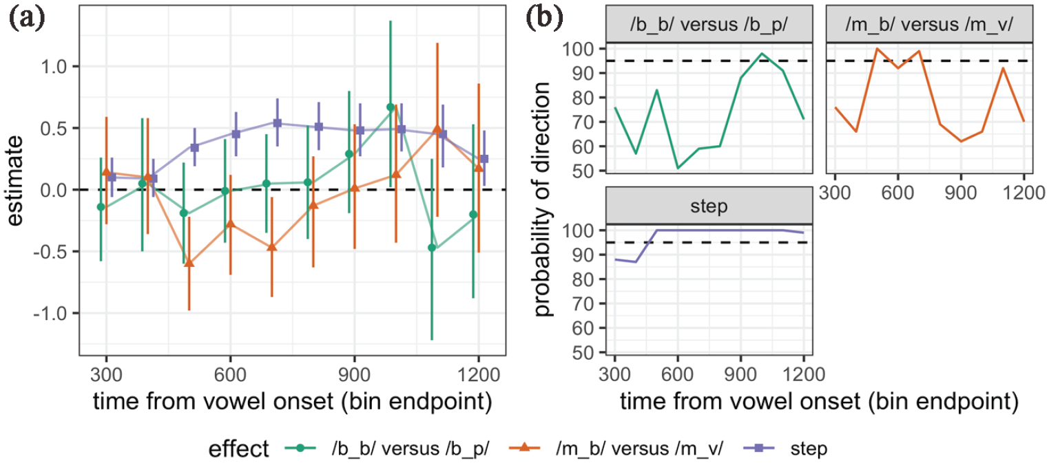
Model estimates and 95% credible intervals for the saccadic moving window analysis, for continuum step, and two pairwise comparisons between (a) frames of interest, and (b) the probability of direction metric for these estimates. The window starts at the time bin containing data for 200–300 ms from target onset, and proceeds in 100-ms intervals (300–400, 400–500, etc.). At time bins at which pd > 95 for a given estimate an effect is taken to be reliable.
As shown in Figure 7, estimates for continuum step reliably exclude zero for the 400–500 ms bin in the time series. That is, listeners reliably responded to the vowel continuum within 400–500 ms after the target vowel onset. This is slightly slower than previous reports for the use of intrinsic spectral cues; for example, Kingston et al. found a reliable effect of vowel acoustics in the 300–400 ms time bin window in their analysis (cf. Reinisch & Sjerps, 2013). We attribute this delay to listeners’ possible reliance on vowel duration as a cue to the /ε/-/æ/ contrast. In our experiment the duration of the vowel was also longer (260 ms) compared with that in previous studies (approximately 170 ms in the case of Kingston et al.). The delay could also be driven in part by the biased nature of the continuum. Regardless of the reasons for the discrepancy, the timing for use of vowel-intrinsic spectral cues provides a baseline for evaluating the effects for frames of interest. We can additionally see that the effect of step in generating new saccades persists throughout the analysis window (in similar fashion to Kingston et al.’s step effect).
Turning to the effect of BP-manipulating frames /mVb/ versus /mVv/, we can see that evidence for an effect of BP emerges at the same time as that of continuum step: 400–500 ms. The effect weakens in the 500–600 ms time bin, but is robust again in the 600–700 ms time bin. BP information only impacts new fixations at these time points, unlike the effect of continuum step. Consider again that because the vowel is 260 ms in duration, information about the coda consonant is available only at that point. Given that it takes approximately 200 ms to initiate a saccade (Dahan et al., 2001; Matin et al., 1993), this effect’s timing suggests listeners rapidly integrated coda consonant information with their perception of the vowel. The 400–500 ms time bin represents the earliest point at which we would expect to see a BP effect (the earliest possible time being 460 ms). Note that the absolute value of the timing of the effect in this experiment is about 100 ms longer than that reported in Kingston et al. (2016), which is consistent with the difference in vowel duration between our stimuli and theirs (260 ms here vs. 170 ms in Kingston et al., Experiment 4a).
Finally, turning to the effect of ND-manipulating frames /bVb/ versus /bVp/, we see there is only one time bin in which the ND manipulation impacts new fixations, the 900–1,000 ms time bin. In looking at Figure 7(a), this time window is the one with the most separation between /bVb/ and /bVp/ frames in line with the ND effect, though the separation is still very slight. This gives some evidence for a temporal asymmetry: the BP effects is rapid, while the ND effect is weaker (smaller and noisier), and delayed in time. This delay is consistent with Newman et al.’s reaction time findings described above.
Although not a focus of interest here, we can note that the effect of initial consonant was also robust and early, as assessed in the moving window analysis. The pairwise difference between /m/- and /b/-initial frames were credible even in the 200–300 ms and 300–400 ms windows, that is, even before the effect of continuum step, as might be expected for effects relating to the initial consonant. Such early effects are unlikely to be related to neighborhood density.
We note here that the traditional moving window analysis (contained in the online OSF repository) largely comported with these results: continuum step had an effect from 400 to 500 ms until the end of the analysis window. BP manipulating frames differed from one another at one time bin later in the moving window: from 500 to 600 ms until the end of the analysis window. The difference between the ND manipulating frames was credible with pd > 95 from 1,000 to 1,100 ms to the end of the analysis window, lining up with the delayed saccadic effect described above.
4.5.2.2 GAMM analysis
Because the GAMM analysis provides more fine-grained information about the time course of an effect (bins are 20 not 100 ms) and takes into account the relationship between adjacent time bins, we used it to evaluate the interaction between continuum step and the BP and ND effects. We expected only early effects on sensory processing to interact with the bottom-up information in the signal as exemplified by the continuum steps. To assess the extent to which continuum step and consonant frame interacted in our GAMM analysis, we compared our model fit with the combined frame and step term to one in which step and frame each had separate smooths which did not interact, using the compare_ML() function in itsadug. The model allowing for an interaction between continuum step and consonant frame provided a better fit to the data (χ2(53) = 299, p < .001; see the open access repository for the full code for model comparison).
In Figure 8 we plot the difference smooths between consonant frames of interest, that is, comparing /mVb/ to /mVv/—the BP effect, and /bVb/ to /bVp/—the ND effect, at each continuum step. These model estimates represent the difference between two smooths, with confidence intervals. The time when this estimated difference reliably becomes non-zero, that is, when the confidence intervals for the estimate exclude zero, is when an effect is taken to be reliable (see, e.g., Steffman, 2021; Zahner et al., 2019). As shown in panel A of Figure 8, we see a robust divergence from zero at all continuum steps for the BP effect arising from the comparison between the /mVb/ and /mVv/ frames. There was a relationship between continuum step (vowel acoustics) and the timing of the effect. Specifically, the biphone probability information was more rapidly integrated when vowel information was more /ε/-like (Steps 6 and 7), than when it was /æ/-like (Steps 4 and 5), though Step 6 showed an earlier effect than Step 7. This sensitivity of the BP effect to fine-grained differences in vowel acoustics is consistent with the claim that it is an early influence on sensory processing. In the context of an /æ/ biased experiment, acoustic evidence for /ε/ would support listeners’ integration of /ε/ with the coda consonant favoring a high biphone probability sequence: in other words, when both the vowel acoustics and consonant frame favor /ε/, divergence based on consonant frame occurs more quickly. The relationship between vowel acoustics and the timing of the BP effect may also offer an explanation for the two time bins (400–500, and 600–700) in which the BP effect led to new fixations on the target, where the earlier time is primarily for the more /ε/-like continuum steps.
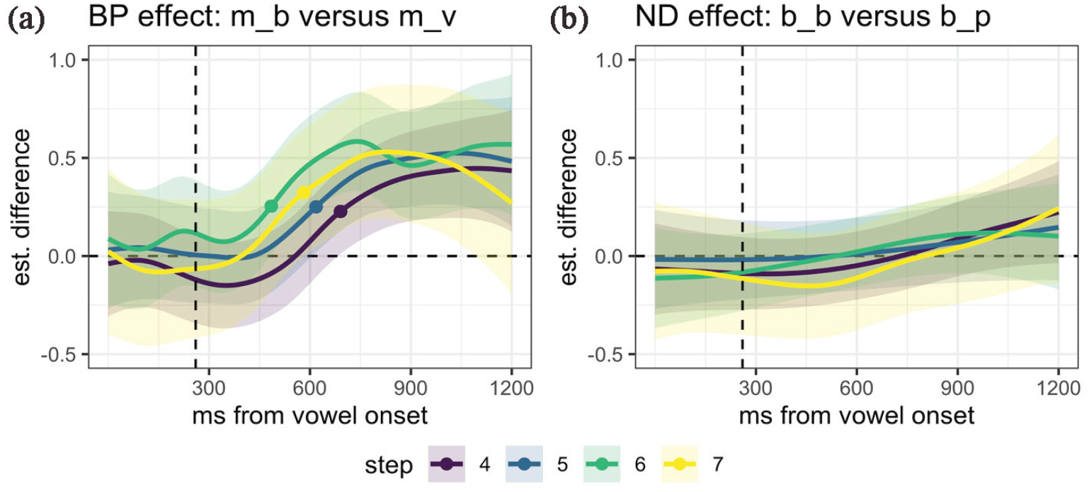
Difference smooths for consonant frame pairs (a: /mVb/ vs. /mVv/; b: /bVb/ vs. /bVp/). The circular point on each trajectory in panel (a) indicates when it has diverged from zero (see text). Step 4: 703 ms, Step 5: 618 ms, Step 6: 484 ms, Step 7: 582 ms). The dashed vertical line indicates the vowel offset (260 ms).
This BP effect was as early as 484 ms from target vowel onset. In contrast, the neighborhood density effect represented by the difference smooth comparing /bVb/ and /bVp/ frames in Figure 8, panel B did not diverge from 0 at any point in the analysis window. That is, we did not observe an ND effect online, lining up with listeners’ click responses, though conflicting with the moving window models.
In summary, the GAMM analysis allows us to confirm (1) a robust and rapid influence of biphone probability in online processing, and (2) a lack of a robust influence of neighborhood density, suggesting that the effects for ND in the moving window analysis are weak and transitory. We further saw that vowel acoustics were integrated with BP information, that is, more acoustic support for /ε/ (in an overall - /æ/-biased experiment) led to an earlier influence of biphone probability.
In Experiment 6, we probed the unexpected difference between the /m/- and /b/-initial frames further, to confirm that this effect is not attributable to BP or ND differences.
5 Experiment 6
Recall that the stronger /æ/ bias for /b/-initial frames observed in Experiment 5 was consistent with the small neighborhood density difference favoring /b/-initial compared with /m/-initial frames. However, its early timing as well as the difference in magnitude of the effect compared with the neighborhood density effect observed in Experiment 4 led us to hypothesize that this effect was not driven by the neighborhood density differences. Instead, we conjectured that the frame effect was driven by perceptual adjustments related to nasal consonants and their effects on judgments of vowel height. Experiment 6 was designed to confirm that the difference between /m/- and /b/-initial frames seen in Experiment 5 was unrelated to neighborhood density and biphone probability. In Experiment 6, we presented listeners with another /m/-initial and /b/-initial frame where both biphone probability and neighborhood density predicted the opposite of the observed difference between /m/- and /b/-initial frames seen in Experiment 5. If we replicate the nasal versus oral frame effect from Experiment 5 here, we can be sure that it was not driven by either biphone probability or neighborhood density differences.
5.1 Materials
The frames used in Experiment 6 were /mVv/ (used in Experiments 3 and 5) and /bVv/. To create the new /bVv/ frames, the initial /b/ from the continua used in Experiment 4 was cross-spliced, replacing the /m/ in the /mVv/ frames. As shown in Table 3, both biphone probability and neighborhood density predict that /bVv/ should show increased /ε/ responses relative to the /mVv/ frame. This is the opposite of the effect seen in Experiment 5 (where the /b/-initial frames showed decreased /ε/ responses), and accordingly, we can test if the effect observed there is independent of both biphone probability and neighborhood density.
Lexical statistics and biases for the continuum endpoints used in the Experiment 4.
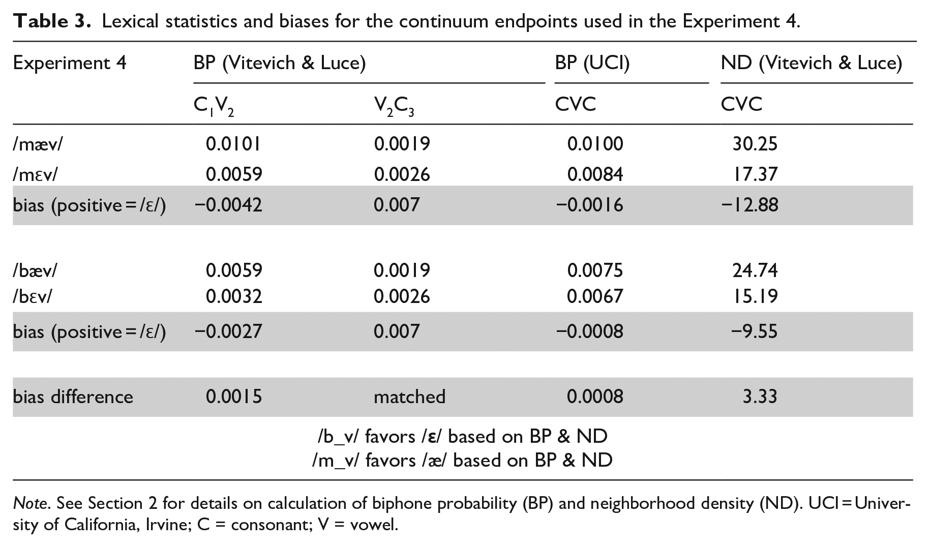
Note. See Section 2 for details on calculation of biphone probability (BP) and neighborhood density (ND). UCI = University of California, Irvine; C = consonant; V = vowel.
5.2 Participants and procedure
Thirty-two self-identified monolingual English-speaking participants were recruited to participate in Experiment 6. One participant was excluded by the metric described in Section 2.6, retaining 31 for analysis. Participants were recruited online, via the platform Prolific, and completed the experiment over the Internet. Participants were instructed to complete the experiment seated in a quiet room with a pair of headphones. Participants were paid $4 USD for this experiment, which took 15–20 min to complete. The experimental procedure was otherwise identical to that in Experiments 1–4.
5.3 Results and discussion
Listeners’ categorization responses were assessed by the same method and model structure as used in previous experiments. In contrast coding the frames, /mVv/ was mapped to −0.5 and /bVv/ was mapped to 0.5. Continuum step had a credible effect on responses, as seen in all previous experiments (β = 3.88, CrI = [3.26,4.50]; pd = 100%). In addition, consonant frame had a credible effect (β = −0.51, CrI = [−0.94, −0.06]; pd = 99%). Replicating the effect observed in Experiment 5, listeners showed decreased /ε/ responses for the /bVv/ frame, as shown in Figure 9. There was some evidence for an interaction between consonant frame and the quadratic term for continuum step (pd = 94); evident in the larger separation based on frame in the middle region of the continuum. The interaction between the linear term for step and frame was not credible (pd = 63).
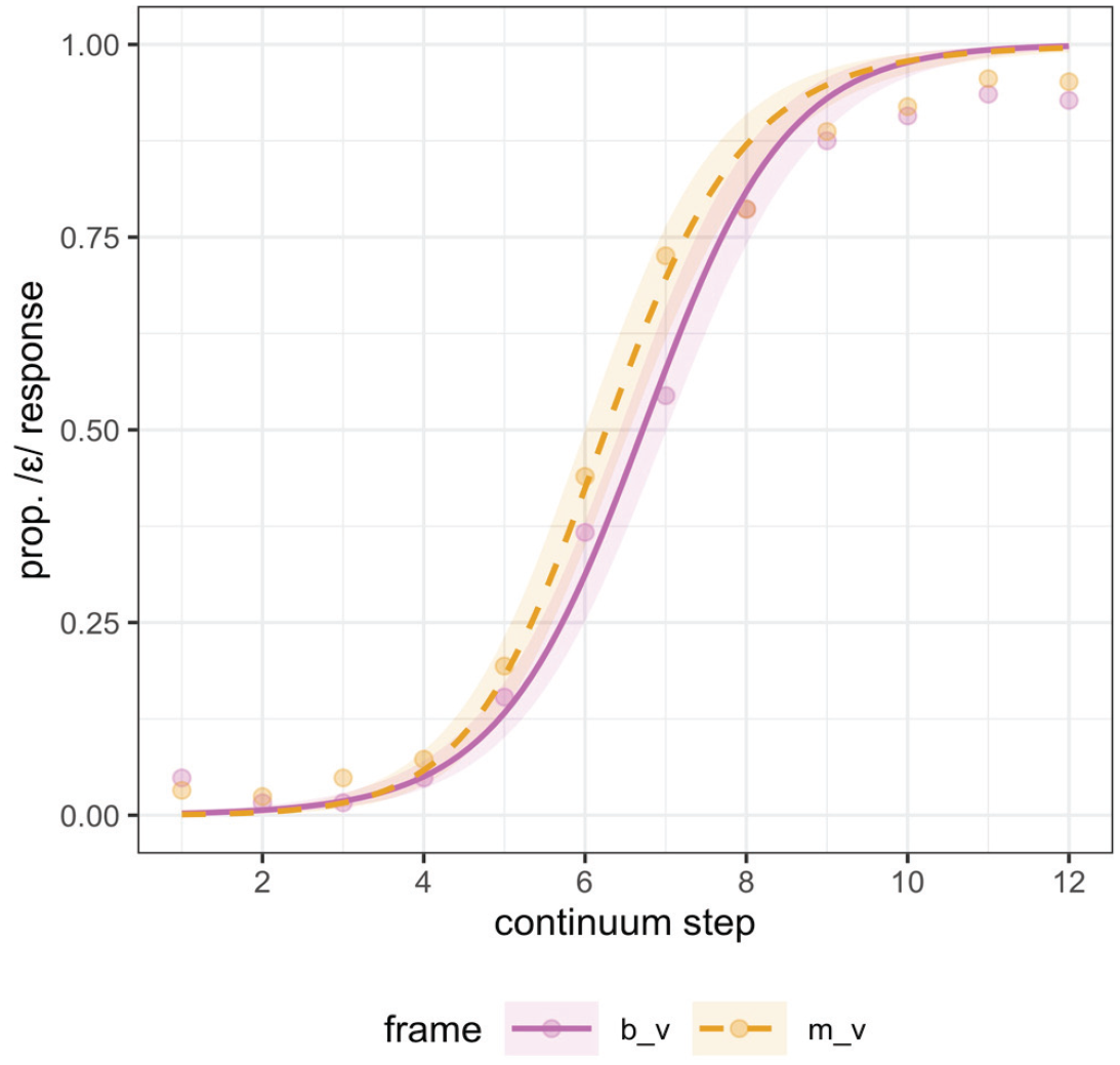
Experiment 6 categorization responses along the continuum, split by consonant frame.
The direction of the effect of consonant frame in this experiment, despite opposing neighborhood density and biphone probability effects, confirms that the robust difference between /m/-initial and /b/-initial frames in Experiment 5 was not driven by differences in neighborhood density (or biphone probability).
6 General discussion
In six experiments, we tested how differences in biphone probability and neighborhood density influence listeners’ categorization of a vowel continuum embedded in nonwords. Listeners in Experiments 1 and 3 shifted categorization to form a high probability sequence even when stimuli were controlled for neighborhood density. Listeners in Experiments 2 and 4 shifted categorization to favor a denser neighborhood even when stimuli were controlled for biphone probability (though the effect was weak in Experiment 4). Finally, in Experiment 5, we used eye-tracking and found evidence for a robust and early influence of biphone probability. In contrast, density effects did not affect categorization and showed only very weak, and delayed effects on looking behavior (in the moving window analyses, but not in the GAMM analysis). In one additional experiment, we probed an unexpected influence uncovered in Experiment 5. This effect resulted from mixing the stimuli from Experiments 3 and 4, and was not driven by either biphone probability or neighborhood density; instead, it was likely due to the influence of an initial nasal consonant.
Our results provide both direct and indirect evidence for a dissociation between biphone probability and neighborhood density effects. In Experiments 1–4, we showed that both biphone probability and neighborhood density exert an independent influence on offline categorization. That is, despite the correlation between biphone probability and neighborhood density in English, biphone probability effects on phonetic processing cannot be explained by differences in neighborhood activation alone as we show in Experiments 1 and 3. Similarly, neighborhood density effects on phonetic processing can also not be explained by differences in biphone probabilities alone, as we show in Experiments 2 and 4.
Categorization data from Experiment 5 also provided evidence for a dissociation, albeit indirectly. In Experiment 5, the mixing of stimuli from Experiments 3 and 4 increased the variability of frames (which had a clear effect on responses as confirmed in Experiment 6). Despite the inclusion of more variable frames in Experiment 5, the biphone probability effect on categorization was replicated from Experiment 3. However, neighborhood density influences, which were small in magnitude in Experiment 4, disappeared when an irrelevant dimension of variation (in the initial consonant) was introduced into Experiment 5. That is, biphone probability effects were robust across online and offline tasks, and not affected by the increased variability in Experiment 5. In comparison, the increased variability in frames and task complexity in Experiment 5 led listeners to largely disregard neighborhood density differences in the stimuli. Together, these categorization results are consistent only with accounts where both biphone probability and neighborhood density independently influence processing, albeit in qualitatively distinct ways.
Independent contributions of BP and ND effects seen here provide clear constraints on existing models of spoken word recognition. This is problematic for models like TRACE that do not independently represent biphone probability information (cf. Pitt & McQueen, 1998). This is also incompatible with Norris et al.’s (2000) proposal that neighborhood density effects are rooted in biphone probability differences. Instead, to account for our results models like Merge (Norris, 1999; Norris et al., 2000) and Shortlist (Norris, 1994) must incorporate information from the lexicon to capture effects of ND on phonetic processing.
In addition, the categorization results from Experiment 5 suggest that biphone probability and neighborhood density affect processing at different times. A general consensus in the literature is that early influences in processing are not impacted by task factors (e.g., Miller & Dexter, 1988), including the presence of orthogonal variation in stimuli of the kind introduced in Experiment 5 (Green et al., 1997), as well as cognitive load (Bosker et al., 2017). Thus, based on robustness across tasks and stimulus variability, it is likely that biphone probability, but not neighborhood density, affects processing early.
The eye-tracking data from Experiment 5 directly confirmed that biphone probability effects are indeed early; biphone probability information was incorporated as early as 400–500 ms after the onset of the vowel, in the same time window as the vowel-internal formant effect. Furthermore, when the vowel formants were more /ε/-like (Steps 6 and 7 on the continuum), biphone probability information was integrated earlier in processing.
The time course of the biphone probability effect in our experiments is similar to the timing of the effect in Kingston et al.’s (2016) findings. In their experiments as well as in Experiment 5, biphone probability effects emerged less than 50 ms into the coda consonant (accounting for the time needed to program a saccade). Given that our biphone probability results cannot be attributed to lexical influences because our continuum endpoints were nonwords, and neighborhood density was matched, we take these converging time course results to strengthen our argument that biphone probability differences may be responsible for Kingston et al.’s findings in Experiment 4a.
The independence of the biphone probability effect, and its early timing, both preclude biphone probability effects from being an epiphenomenon of lexical feedback (cf. Newman et al., 1997). Instead, the rapid, independent biphone probability effects observed here are consistent with proposals that biphone probability affects the sensory activation of phones, and its influence varies as a function of the robustness of the speech signal (Norris et al., 2000; Pitt & McQueen, 1998; Pylkkänen et al., 2002).
In addition to dissociating biphone probability and neighborhood density effects on offline categorization performance, we also found robust evidence for an early biphone probability effect on online processing. What was less compelling was the evidence for a late neighborhood density effect during online processing. Recall that neighborhood density effects in Experiment 5 were not present in the categorization data, nor in the GAMM analysis, though they were observed late in both the saccadic and traditional moving window analysis. Future eye-tracking experiments will be required to confirm if neighborhood density effects are truly as delayed as might be expected if they are a result of feedback (Luthra et al., 2021; Newman et al., 1997), or only moderately so as expected if they feed forward to decision nodes (Norris et al., 2018). Note that in this paper, we use feedback to reference lexical influences on online processing only; this is distinct from some current proposals where feedback may be used to learn speech sound categories during acquisition (Nixon, 2020; Nixon & Tomaschek, 2021) and other perceptual learning (Norris et al., 2003, 2016).
In the aggregate, based on the lack of robustness of neighborhood density effects, we can rule out the possibility that it affects processing as early as biphone probability. Early biphone probability effects that are independent of neighborhood density, as we demonstrated in our experiments, are compatible with several proposals about the representation and acquisition of sound categories. Biphone probabilities could be learned purely from the clustering of acoustic tokens without access to word-level information (Feldman et al., 2013; Maye et al., 2002) as has been demonstrated computationally (Cairns et al., 1995; Norris, 1993). They can be learned when sound categories and words are learned jointly as well (Feldman et al., 2013) as Norris (1993) shows. Similarly, independent, and early biphone probability effects are also compatible with exemplar model architectures (Nosofsky, 1986; Shi et al., 2010) and a discriminative lexicon (Baayen et al., 2019). They are able to do so because the input in all these proposals is a long enough acoustic signal that encompasses biphone probability information.
In both exemplar and discriminative approaches, neighborhood density effects can be captured by competition among to-be-recognized items. Exemplars in denser neighborhoods may be presumed to be in a more densely populated exemplar cloud, though to our knowledge, possible metrics capturing this property have not been used in the literature to make explicit time course predictions. In a discriminative lexicon “activation diversity” has been proposed as a metric to capture the extent of the input’s contact with multiple items in the lexicon, and thus, represent uncertainty (Arnold et al., 2017; Tomaschek et al., 2021). To the extent that “uncertainty,” operationalized in some fashion, is correlated with slower processing, activation diversity in a discriminative approach may offer another lens into understanding what we have described in terms of activation and competition dynamics among lexical candidates. However, it is not clear what explicit time course predictions may arise from this approach. In addition, because activation diversity as a metric has been used to explain segmental durations in speech production (Tomaschek et al., 2021; Tucker et al., 2019), it is unclear how neighborhood density effects in perception, as explored in the present study, may be captured in these models (Arnold et al., 2017). In any case, exemplar models as well as discriminative learners are feedforward models. Thus, if neighborhood density effects stem from feedback instead of feedforward activation, this poses a problem for both.
In conclusion, we present new evidence for the dissociation of biphone probability and neighborhood density effects using a combination of categorization and online processing measured with eye-tracking. Our results offer support for the claim that biphone probability influences in perception are independent from that of neighborhood density, such that only biphone probability affects early, sensory processing of phones. Based on these results, we argue in favor of models that encode both biphone probability and neighborhood density, albeit with asynchronous timing effects on early processing. Further research will be needed to establish a precise time course for neighborhood density effects, and to determine how they combine with other known influences, such as word-hood and word frequency.
Footnotes
Acknowledgements
The authors thank Adam Royer and Kate Sandberg for recording the materials for the stimuli.
Funding
The author(s) disclosed receipt of the following financial support for the research, authorship, and/or publication of this article: This research was partially supported by NSF BCS-2214017 to M.S.