
Abstract
Researchers often need to justify their choice of sample size, particularly in fields such as animal and clinical research, where there are obvious ethical concerns about relying on too many or too few study subjects. The common approach is still to depend on statistical power calculations, typically carried out using simple formulas and default values. Over-reliance on power, however, not only carries the baggage of statistical hypothesis tests that have been criticized for decades, but also blocks an opportunity to strengthen the research in the design phase by learning about challenges in interpretation before the study is carried out. We recommend constructing a ‘quantitative backdrop’ in the planning stage of a study, which means explicitly connecting ranges of possible research outcomes to their expected real-life implications. Such a backdrop can facilitate a priori considerations of how potential results, for example represented by intervals, will ultimately be interpreted. It can also serve, in principle, to help select single values of interest for use in traditional power analyses, or, better, inform sample size investigations based on the goal of achieving an interval width narrow enough to distinguish values deemed practically or clinically important from those not representing practically meaningful effects. The latter bases calculations on a desired precision, rather than desired power. Sample size justification should not be seen as an automatic math exercise with a right answer, but as a nuanced a priori investigation of measurement, design, analysis and interpretation challenges. Construction of the quantitative backdrop provides a tangible starting place for such an investigative process.
Study proposals, particularly for animal and clinical research, typically require justification for a proposed sample size based on statistical power calculations, which are often carried out automatically under defaults in web applets or statistical software. The cost-benefit analysis of this effort to researchers needing funding is easy, and following the usual procedure typically requires little, if any, justification. In our view, however, the foundations of statistical power deserve less blind acceptance and more healthy interrogation by researchers and reviewers.
We see research design as an underemphasized part of the research process and support the expectation that researchers meaningfully justify sample size choices—particularly when there are ethical concerns, such as in animal research. When taken as more than default mathematical calculations, sample size investigations can motivate deeper evaluation of plans for study design, analysis and interpretation, and expose limitations early enough to promote improvement while taking advantage of the subject matter expertise and creativity of researchers. Before we discuss an alternative path, we visit some concepts we are implicitly trusting by relying on statistical power.
This short communication does not provide yet another tutorial of sample size calculations meant to return a clear-cut answer to the question of exactly how many participants are needed per group; instead, it is meant to spark more critical evaluation of measurement, design, analysis and interpretation in the research design phase, before resources (including animal lives) are used to carry out the study.
Before discussing power-related concepts, it is important to acknowledge that the underlying concepts are subtle and intricate, making it nearly impossible to simplify them sufficiently for a broad audience without losing technical correctness. This point actually underlies much of our criticism of power-based justifications because users, and even teachers, are often not choosing to rely on statistical power with adequate understanding or appreciation of the concepts involved. For example, in the following, we are referring to ‘test hypothesis’ rather than ‘null hypothesis,’ because the tested hypothesis should not automatically amount to a nil, zero or no-effect hypothesis. 1 We can and should also consider non-zero values, and we often do this already because our traditional 95% confidence intervals show all hypotheses (possible values for the true effect size) that would result in a p-value greater than 0.05 when tested using the same data and background model (Box 1).
The ‘coverage’ rate definition of a 95% confidence interval describes the procedure that generates observed intervals that contain (‘cover’) the true value 95% of the time—given all assumptions of the procedure are met. Another way to think about it is that 95% of the hypothetical confidence intervals constructed from theoretical data sets generated under the procedure (which includes design, model and analysis) contain the true value; 5% of such intervals are expected to be ‘errors’ in terms of excluding the true value, given all assumptions are met.
Confidence intervals can be created by inverting hypothesis tests: a 95% confidence interval includes all values for the test hypothesis (all possible values for the true effect size) that would result in p-values larger than 0.05 and would thus not be ‘rejected’ according to a strict decision rule, given the data and the statistical model with all background assumptions. The interval can thus be taken as conveying the effect sizes that are most compatible with the data and model and can therefore be termed a compatibility interval.5,15,16
Intervals matching classic confidence intervals can arise more generally as quantiles or percentiles summarizing the most common values of a distribution without any need for referencing a true value or defining an error rate. This is the motivation for using posterior intervals within Bayesian inference as summarizing the region of a posterior distribution with largest posterior density (typically the middle of a distribution). In a non-Bayesian setting, intervals can be used to summarize randomization distributions or sampling distributions, again with no reliance on true or hypothesized values or error rates. A 95% interval, for example, typically provides the interval excluding values beyond the 97.5 percentile and below the 2.5 percentile that would be considered ‘rare’ according to the chosen criterion.
We encourage this more general ‘summarizing a distribution’ interpretation that helps relax interpretation of the endpoints from hard-boundary thresholds to rather arbitrary and user-chosen summaries of a distribution of interest. Displaying intervals as a collection of segments representing different choices for percentiles (e.g., 95% and 80%) facilitates this view (Figure 1).
The goal is to have a more general interpretation of intervals beyond error and coverage rates that allows their (necessarily imperfect) use as a way to represent the values most compatible with the data and the model with all background assumptions in a way that also honors context-dependent knowledge.
Entering the hypothetical land of error rates
Opening up the baggage of statistical power starts with interrogating the concepts of type I and type II error rates. Under a hypothesis-testing statistical framework, errors are defined relative to a simple decision around whether to reject the test hypothesis—it is either rejected in error (‘reject when we should not’) or not rejected in error (‘fail to reject when we should’). The former is a type I error, the latter is a type II error, and power is the rate of rejection of an incorrect test hypothesis (‘rejecting when we should’), the non-error compliment to a type II error. Power calculations are based on long-run rates of these errors over hypothetical study replications: type I error rate (α), type II error rate (β) and power (1 – β).
Error rates (as opposed to single errors) are therefore conceptually based on a hypothetical collection of many decisions, a proportion of which are errors. The collection of decisions is hypothetical because the decisions would arise from many study replications that in real life are not conducted; thus error rates are hypothetical—and these are the fundamental ingredients underlying power calculations used to justify real-life research decisions. While we appreciate the theoretical attractiveness and mathematical convenience error rates offer, we question handing them too much authority. They seem to bring an air of objectivity and comfort to an otherwise challenging and messy research process; but their roots inhabit the same soil as statistical hypothesis tests that have been criticized for decades, for example for their rigid focus on often poorly justified null hypotheses and decision rules.2–5
Problems arising back in reality
When we leave the hypothetical land of a having a collection of data sets and associated decisions about rejecting a test hypothesis, we inevitably face issues: real-life error rates are unknown and difficult to fully conceptualize—we usually do not have data from multiple study replications, and we never know whether the decision about rejecting a hypothesis is in error for any individual study. In addition, theoretical error rates are only as trustworthy as the assumed model of the process that generated the real-life data—and this statistical model is inherently based on assumptions about reality that are usually violated in practice and uncertain by definition (otherwise they would not be called assumptions).
While similar cautions apply broadly for statistical methods, in power-related practices we often see blatant ignoring of the underlying model and its connection to theoretical error rates, leading to overconfident expectations about reality and questionable study design decisions. This is exemplified by misleading statements such as ‘we will be wrong 5% of the time’ if we reject a test hypothesis based on a p-value threshold of 0.05; this statement would only be true if the statistical model and all its assumptions were correct— but there are countless explicit and implicit assumptions that are part of a statistical model, 6 so a statement that uses the word ‘will’ is overconfident in almost all cases. The same applies to ‘we will obtain a statistically significant result in 80% of cases’ if power is 80%, which is misleading for the same reasons stated above. Further, power is not the ‘probability of obtaining a statistically significant result,’ as is often stated; it is this probability only if the true effect is exactly equal to the alternative hypothesis used for power calculation and if all other model assumptions are correct, which is typically far from reality.
In general, power calculations beg a lot of trust in unknowns and misunderstood concepts, and yet it is common to treat resulting sample size numbers as if they provide concrete and objective answers to inform crucial research decisions, often ones with ethical implications. We hope this glimpse into the baggage associated with error rates, and thus power, will spur some healthy skepticism; but motivating change must also acknowledge the unfortunate reality that incentives from peers, funding bodies and animal welfare committees promote the comfortable status quo (whether explicit or only assumed by the researchers) instead of rewarding curiosity about limitations of current methodological norms. Pushback against dichotomous statistical hypothesis testing has gained traction within analysis,4,5 but influence on use of power calculations has been limited, despite reliance on the same criticized theory and practices. 7 An over-focus on simple statistical power also inadvertently encourages ignoring more sophisticated design and analysis principles available to increase precision (and thus decrease, for example, number of animals used), because calculating statistical power for more complicated designs and analyses is often not straightforward or not implemented in default statistical procedures.
An alternative definition of success tied to research context
It is possible to let go of much of the baggage of error rates by shifting away from defining a research ‘success’ in terms of avoiding theoretical type I and type II errors toward a context-dependent success that honors inevitable gray area in interpretation instead of, for example, forcing use of single values for null and alternative hypotheses. A successful study should result in useful information about how compatible the data (and background assumptions) are with values large (or small) enough to be deemed practically important (e.g., clinically relevant) as compared with values too small (or large) to be considered practically important. We can do what we can in the design phase to make such a success possible, but of course there is no way to avoid results potentially consistent with the gray area between the two regions; this is not a problem, it simply highlights the challenges in interpretation that exist in real life but often are hidden behind use of default criteria and assumptions in common methods.
For example, suppose the effect of a new anti-hypertensive drug on average systolic blood pressure has to be a reduction of at least 10 units to be deemed clinically relevant, with a reduction of 6–10 units representing gray area (unclear clinical relevance), and fewer than 6 units clearly not clinically meaningful (though clearly not ‘no effect’). Then, a sample-size related goal might be to achieve a precision such that an interval is not wider than 4 units. That is, we aim for obtaining an interval that cannot overlap both clinically relevant (values greater than 10) and not relevant values (values under 6), which is only possible if an interval is narrower than 4 units (Figure 1). Note that such a successful research outcome can accompany very large or very small p-values and thus is not defined by ‘statistical significance.’
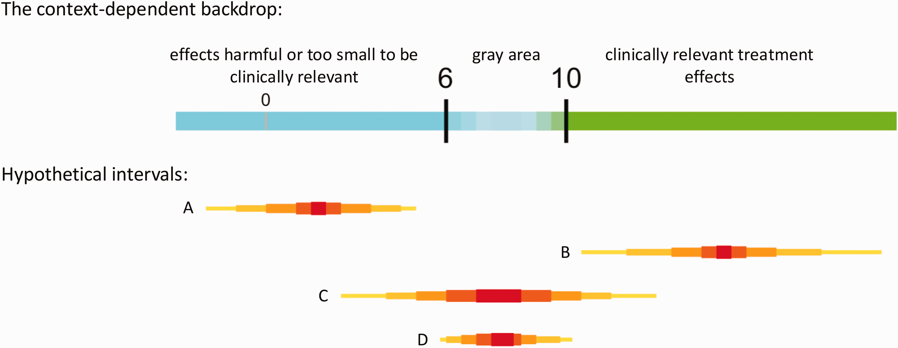
Example of a ‘quantitative backdrop’ with hypothetical intervals that could arise after data collection and analysis. The number-line backdrop is context-dependent and honors a realistic gray area in which clinical relevance is unclear. The backdrop facilitates meaningful interpretation of potential study results and highlights the goal of designing a study to provide an interval of values (those reasonably compatible with the data, given the model 5 ) in either the blue or green region, not both regions simultaneously. Intervals A and B would be successful in helping to distinguish between effects too small to be clinically relevant and those large enough to be clinically relevant. Interval C, on the other hand, would cover values in both regions, meaning the single study failed to distinguish between the two regions associated with different conclusions. We can aim to avoid scenario C by trying to restrict the width of the interval enough so that it cannot contain values on both sides of the gray area (smaller than 6 and greater than 10, for example). Note that even with a desired width, an interval may end up covering the gray area (see D), which, while not a ‘success’ as defined, is valuable information to inform future research and a reality of doing research that is often swept under the rug in commonly used power-based methods where interpretations are treated as black-and-white decisions. Sample size is only one ingredient affecting interval widths, and guidelines on justifying a sample size based on precision can be found elsewhere.8–12 Note that the depicted intervals are actually collections of intervals to better summarize a distribution and can be defined by sets of percentiles (e.g., 99%, 95%, 80%, 50%) deemed useful for the context.
As alluded to in the example, one strategy for a researcher to exert control over the width of a future interval (precision) is through choice of sample size; more information and technical guidance on choosing a sample size based on precision rather than power can be found elsewhere.8–12 Although precision-based approaches can be carried out in ways just as automatic and default as traditional power-based approaches, the focus on intervals invites use of context-dependent knowledge and expertise related to the treatment and proposed methods of measurement. In this spirit, we offer a larger framework for incorporating research context and interpretation of results a priori.13,14 The framework allows for a priori considerations of how different intervals will be interpreted in context, and although it can be used to support precision-based sample size investigations, it is not offered as simply a sample-size calculation method.
A picture can help clarify alternative definitions of success (Figure 1): intervals A and B clearly distinguish between regions of different practical implications, and both are considered study successes because all values in A are deemed too small to be clinically relevant, and nearly all values in B are large enough to be clinically relevant. Interval C, on the other hand, is not considered a success because it contains values in both regions, not supporting a conclusion in either direction. Narrower intervals (greater precision) help to avoid scenario C and facilitate successes (A and B). Even with a narrow interval, we can still land partially or fully in gray area (D); while potentially frustrating, such is the reality of doing research and D still provides valuable information to inform future studies or meta-analyses.
As Figure 1 conveys, this approach requires initial context-dependent work to draw the number line ‘backdrop’ delineating the regions. Assigning practical or clinical importance to values a priori can be compared with creating a backdrop in theatre productions—a picture hanging behind the action of a play to provide meaningful context. In research, a ‘quantitative backdrop’ provides a contextual basis in front of which study design, analysis and interpretation of results take place, 14 ideally without over-reliance on arbitrary default statistical criteria. While simple in construction, the process is not trivial and can be surprisingly challenging, partly because it is a novel exercise for most researchers and statisticians.
While the backdrop framework can help support and facilitate sample size investigations, it is broader than that and need not involve sample size calculations to be useful. For example, suppose researchers are planning to use the largest sample size possible given ethical, logistical or cost constraints and have done as much work as possible to decrease background variance through design and analysis decisions. The result of the planning exercise is an interval with an approximate width that can be compared with the quantitative backdrop to think about and articulate how intervals will be interpreted as their location moves relative to the backdrop. The exercise can help make decisions about whether the research is worth carrying out given the width of an interval that can possibly be achieved and can serve justification of interpretations after data collection and analysis if the a priori interpretations are appropriately documented (e.g., pre-registered).
Loosening our grip on interval endpoints
Our use of the term ‘interval’ thus far has been purposefully vague, as our definition of success does not depend on any particular method for obtaining intervals (e.g., confidence, credible, or posterior intervals), only that the researcher sufficiently trusts the interval and can justify its use to others (Box 1). We promote relaxing long-held views of what a statistical interval does, or should, represent and see interpreting confidence or credible intervals as compatibility intervals as a step in this direction.1,5,6,15,16 Compatibility encourages a shift from dichotomously phrased research questions (e.g., ‘is there a treatment effect?’) to the more meaningful ‘what values for a treatment effect are most compatible with the obtained data and the model with all background assumptions?’ (to which the answer would be the values included in the obtained interval). 16
We can also relax the rigidity with which interval endpoints are interpreted. When drawing an interval, the line must have ends, but values beyond the endpoints do not suddenly switch from being compatible with the data and assumptions, to incompatible. Values inside the interval are just considered more compatible, and values outside are less compatible, 5 and that applies whether we have a 95% or 80% or any other interval. Loosening our grip on the rigidity of endpoints can facilitate another shift from believing we are calculating the one and only sample size answer to undertaking an investigation that honors limitations and challenges. The technique of using a collection of different quantiles to display the intervals as in Figure 1 can help with this challenge.
The reality is that to carry out a sample size calculation based on precision (via math or computer simulation), we must input a specific interval width. This may at first seem inconsistent with the recommendation to relax interpretations of intervals and rigidity of endpoints. However, there is no conflict if we also relax our belief that there is a single correct answer to the sample size question and instead use the exercise to motivate a nuanced investigation to help understand challenges inherent in carrying out the study. This can include many calculations to reflect different levels of precision and varying sensitivity to assumptions.
As mentioned previously, precision-based methods can be used easily to carry out a typical power calculation in disguise, rather than the more holistic approach we are promoting. Several practices can help avoid using them as power calculations in disguise: (1) avoid using confidence intervals to carry out hypothesis tests by simply checking whether they contain a hypothesized value (usually the null hypothesis of no effect); (2) embrace the a priori work of developing the context-specific backdrop identifying the range of values to be considered practically, or clinically, relevant, as well as the gray area between; (3) create the backdrop using a scale that facilitates practical interpretation within context (e.g., not standardized effect sizes) and (4) contrary to common advice, do not simply use a previously obtained estimate to define the ranges of values in the backdrop (e.g., the 6 or the 10 in Figure 1).
The last point deserves further attention. It is common to use previous effect estimates (such as pilot study results) as the ‘(practically meaningful) alternative value’ in traditional power calculations, although this is not necessary or recommended. The practice has negative implications for sample size justification, 11 for example, because published effect estimates are often exaggerated. 17 Such practice can lead to sample sizes that are smaller than needed (if the previous estimate is larger than the smallest values deemed practically relevant) or larger than needed (if the previous estimate is smaller than what is deemed practically relevant). There is no reason a previous estimate should automatically be judged practically relevant—it can fall anywhere relative to the backdrop and should not change the a priori developed backdrop! Note, however, that previously obtained estimates of background variance (e.g., the width of previous intervals) are valuable for design decisions and sample size investigations.
Creating a quantitative backdrop is not an exercise in guessing the actual effect, but an exercise in explicitly defining and sharing the context within which an estimated effect will be interpreted. This can be confusing because it is counter to what is often taught and expected from funding agencies. Relative to the previous example, a pilot study may have produced an estimated reduction of three units, which, when considered relative to the backdrop, is not clinically relevant and therefore there is no reason to justify increasing the sample size to attempt to estimate an effect as small as three units with sufficient precision. The decision of what values will be judged practically relevant should thus be made based on knowledge of the subject matter (e.g., medical) and of the measurement scale, not on previous estimates of an effect of interest. Defining relevant values can, and should, be carried out before any pilot study, facilitating the exercise of specifying how potential pilot study results will be used for further planning.
Taking back the power shouldn’t be easy
A common question when considering this framework is: what if researchers do not have enough knowledge of how the outcome variable’s measurement scale is connected to practical implications to create the quantitative backdrop? That is, what if they are not able to identify values that would be considered large, or small, relative to practical implications? If this is the case, then we argue researchers should honestly declare that, with the currently available knowledge, it is impossible to come up with a justifiable sample size. In such a situation, using default power calculations will essentially just move the research challenge into the analysis and interpretation phase, after already using valuable resources for the experiment—if practical implications of possible outcomes are unclear before the experiment, they are usually still unclear after results are in. Instead, an inability to identify practical implications of possible outcomes in the planning stage of a study would highlight the exploratory nature of the research and a need for better understanding of the outcome variable, which could be a valuable research goal by itself.
Engaging in a sample size investigation as we are recommending will not feel easy. Investigating sample sizes, rather than calculating them using default power analysis settings will bring up hard questions, throw light on assumptions that were previously hidden, and create additional problems to address. We need constant reminders that statistical methods depend on a substantial set of background assumptions; and methods for justifying sample sizes are no exception.
Sample size investigation presents an opportunity for researchers to give up simple math calculations in exchange for taking back some of the authority and creativity blindly given over to statistical power for decades. We have a responsibility as scientists to work to understand and interrogate our chosen scientific methodologies to the best of our ability to avoid being fooled by our own assumptions. Embracing this challenge in the design phase of a study can lead to higher quality research, and ultimately to more efficient research spending and respect for human and animal lives.