Sage Journals: Discover world-class research

Abstract

Objectives

While there has been significant study of the relationship between police legitimacy and its key antecedents - procedural justice (PJ) and police effectiveness (PE) at the individual level, little attention has been paid to what impacts general evaluations of PJ and PE. Our paper focuses on these perceptions at places.

Methods

Our analyzes utilize survey data collected on 447 street segments in Baltimore City, MD, in two waves. We first used EFA to determine the latent structure of PJ and PE measures. We then used mixed effects OLS regression modeling techniques to examine the antecedents of a “scorecard” of perceptions of the police.

Results

The results of the EFA show a single latent structure that we term the scorecard for PJ and PE. While we find that experiences with the police and street conditions that the police are presumed to impact influence the scorecard, street conditions that are less likely to be influenced by police (collective efficacy and concentrated disadvantage) also have strong influence.

Conclusions

Both the research and policy-oriented literature often view the police as primarily responsible for their public image. Our data suggest that at the place level, such perceptions are also strongly impacted by factors primarily outside police influence.

Keywords

procedural justice police effectiveness crime hot spots micro geographic places

Introduction

Efforts designed to improve the relationship between the police and the public have gained greater urgency in recent years. Examples of police abuse of authority and police shootings, especially of minorities, have led to large scale protests against the police and calls in many cities for “defunding the police,” or at least reducing their role in American communities (e.g., Nix, Wolfe, and Campbell 2018; Vitale 2017). Policy makers and scholars have, to a great extent, focused their proposals for reform around what has come to be termed “police legitimacy” (President’s Task Force on 21^st Century Policing 2015), which focuses on the extent to which citizens trust the police and whether they are willing to obey police authority (Sunshine and Tyler 2003; Tyler 1990, 2004). Using a substantial body of basic research (e.g., Lind and Tyler 1988; Thibaut and Walker 1975), scholars led by Tom Tyler have proposed that short term changes in policing can have meaningful impacts on how the public perceives the police (e.g., Gau et al. 2012; Kochel, Park, and Mastrofski 2013; Reisig, Bratton, and Gertz 2007; Stoutland 2001; Tyler, Schulhofer, and Huq 2010; Tyler and Fagan 2008; Tyler and Huo 2002; Tyler and Wakslak 2004).

These researchers have assumed that there are two main mechanisms that can be marshaled by police to improve police legitimacy. In most studies, “procedural justice” (PJ) has been identified as the strongest antecedent of legitimacy. PJ refers to how police behave during their interactions with citizens. Giving voice to citizens, showing neutrality, treating citizens with respect, and evidencing trustworthy motives, are all seen as essential police behaviors for encouraging police legitimacy (Schulhofer, Tyler, and Huq 2011; Sunshine and Tyler 2003; Tyler 2004, 2009). Police effectiveness (PE) in terms of reducing crime and other problems is a second key antecedent of legitimacy, albeit generally identified as less important than PJ (e.g., Hinds and Murphy 2007; Jonathan-Zamir and Weisburd 2013; Murphy, Hinds, and Fleming 2008; Schulhofer, Tyler, and Huq 2011; Sunshine and Tyler 2003; Tyler 2004, 2009; Tyler, Schulhofer, and Huq 2010). While socio-demographic and other background characteristics may impact views of PJ and PE, they are hypothesized to develop primarily from experiences with the police, either through direct personal encounters, vicarious experiences through family, friends, and neighbors, or as a result of observing activities or outcomes that are associated with policing (e.g., Braga et al. 2014b; Nagin and Telep 2017; Tyler 1990).

At the same time, some scholars have challenged the assumption that police legitimacy can be significantly influenced by policing in the short run (Nagin and Telep 2017; White, Weisburd, and Wire 2018). These scholars suggest that perceptions of the police are a relatively stable factor, rooted in broader perspectives of the law, justice, and historical treatment. Similar to traditions and morals that become embedded in families and communities’ daily lives, according to this view, perceptions of the police develop, in large part, from accumulated vicarious experiences (Augustyn 2016; Rosenbaum et al. 2005) and socialization from generations of interactions with and beliefs about the police (Wolfe, McLean, and Pratt 2017). Nagin and Telep (2017) argue that perceptions of police legitimacy result primarily from an “accumulation of a lifetime of cultural, community, and familial influences” (Nagin and Telep, 2017:7), not from short term experiences. This ongoing debate in the literature raises important questions about the relative roles of police-related versus non-police related considerations in shaping public views of the police, or, in other words, the amount of influence the police have over their public image.

While perceptions of the police have generally been studied at the individual level (e.g., see reviews by Brown and Benedict 2002; Cao and Wu 2019; Decker 1981; Mazerolle et al. 2013a), changes in policing over the last two decades have led to a shift in the orientation of policing from individuals to places. Especially in the case of proactive policing, place-based approaches have become a key strategy of the police that has been buttressed by a strong body of evidence regarding the effectiveness of hot spots policing strategies (see review by Weisburd and Majmundar 2018). For police managers, the question that they are often confronted with is “how can I improve assessments of policing at high crime places?” or “how can I prevent negative reactions to policing in those places where police work is concentrated?” For scholars, the importance of places in crime prevention raises questions not only about how individual attitudes towards PJ and PE are formed, but what street-level characteristics influence average street-level attitudes. This focus echoes recent investigations of the idea of “group-level PJ” (Jonathan-Zamir, Perry, and Weisburd 2021; O’Brien, Tyler, and Meares 2020).

While the key antecedents of police legitimacy are assumed to be heavily influenced by what the police are perceived to be doing and how they are doing it (which is the justification for training police in PJ for example; see Weisburd et al. 2022), there has been little systematic study of what in fact influences place-based evaluations of PJ and PE. This is the focus of our paper. We begin by discussing the significance of PJ and PE in understanding police legitimacy, and then explain the importance of analyzing the antecedents of PJ and PE at the street-segment level. We then review three categories of potential street-level influences on assessments of PJ and PE (experiences with the police, street conditions within police influence, and street conditions largely outside police influence), and detail the specific variables in each category included in our analysis. Based on a factor analysis, we create a combined summary measure of PJ and PE, which we term the “scorecard of policing.” Relying upon two waves of surveys, each including over 3,000 responses on 447 street segments, we examine how changes over a six-year period in characteristics of street segments and perceptions of residents of these street segments in Baltimore City, Maryland, influence street-level scorecard values.

Why are Citizen Evaluations of Procedural Justice and Police Effectiveness Important?

Since Tom Tyler's seminal publication in 1990, Why people obey the law, the concept of “police legitimacy,” commonly defined as “the belief that the police are entitled to call upon the public to follow the law and help combat crime, and that members of the public have an obligation to engage in cooperative behaviors” (Tyler 2004:86–87),¹ has been the subject of thousands of research and policy-oriented publications (for reviews see President’s Task Force on 21^st Century Policing 2015; Weisburd and Majmundar 2018). This exceptional interest developed, in large part, from the appealing idea that outcomes such as compliance and cooperation with the police, acceptance of police authority, willingness to empower the police, and even long-term law obedience, are heavily influenced by public perceptions of the police as a legitimate authority (Mazerolle et al. 2013a; Tyler 2004, 2009).

Given the iconic status of police legitimacy in research and policy discussions, it is not surprising that a key question that has been occupying researchers concerns the roots of legitimacy: how citizens develop trust in the police and willingness to obey police directives. Following Tyler's work (e.g., Sunshine and Tyler 2003; Tyler 2004, 2009), studies addressing this question have typically contrasted subjective views of the fairness embedded in police treatment (PJ) with perceptions of police effectiveness (PE). These studies usually find that both types of evaluations are strongly correlated with the broader view of police legitimacy, while of the two, PJ is more closely related to legitimacy (see reviews by Jackson et al. 2015; Mazerolle et al. 2013a; Nagin and Telep 2017, 2020; Weisburd and Majmundar 2018). At the same time, a question that has received surprisingly little attention concerns how individuals develop their general assessments of police PJ and PE (although see for example Bradford, Jackson, and Stanko 2009; Gau et al. 2012; Pickett, Nix, and Roche 2018; Roché and Roux 2017), and more specifically – the extent to which such evaluations develop from police-related versus non police-related considerations. Alward and Baker (2021:33–34) recently note for example in regard to PJ, “(d)espite the importance of procedural justice for successful police and court processes, additional research is needed to better understand the antecedents of procedural justice perceptions”.

Importantly, in asking how assessments of PJ and PE develop, we are not referring to the four factors (giving voice, showing neutrality, treating people with dignity and respect, and demonstrating trustworthy motives) that have come to be recognized as the constituent elements of PJ (which have been studied extensively as “antecedents” or “predictors” of PJ; e.g., Elliott, Thomas, and Ogloff 2011; Lind, Tyler, and Huo 1997), but to the way these assessments, as well as evaluations of PE, are formed in the first place based on what citizens see, hear, and experience in their daily lives. We are also not concerned here with how assessments of police-provided PJ and PE develop in a specific encounter (e.g., Terpstra and van Wijck 2021; Worden and McLean 2017), but with general evaluations of how fair and effective the police are perceived to be (for a distinction between general and specific PJ see for example Mazerolle et al. 2013b).² Thinking beyond individual experiences, if we accept that general “scores” of police fairness and effectiveness influence views of police legitimacy, understanding how these scores develop, and particularly the extent to which they reflect police conduct versus contextual features beyond police influence, becomes a key issue in understanding the bedrock on which police legitimacy lies.

The Street as the Unit of Analysis

The terms “procedural justice” (PJ), “police effectiveness” (PE) and “police legitimacy” originate from psychological models. Thus, these attitudes and the relationships between them are typically discussed as psychological traits and processes, and analyzed at the individual level. However, there is a long tradition in criminology that assesses community attitudes toward the police (see review by Sampson 2002). Émile Durkheim first raised the importance of community-level attitudes in his proposals regarding a “collective consciousness,” which underlies individuals’ sense of solidarity, belonging and identity, and in essence binds them together into collective units. Collective consciousness is a social phenomenon, not an individual one, which “has a life of its own,” and is reflected, for example, in social norms and institutions. Individuals internalize the shared norms, beliefs and attitudes, and, in turn, behave accordingly in their daily lives (Durkheim 2014; Némedi 1995; Smith 2014). Treating evaluations of policing as a collective trait is also supported by a recent observation made by O’Brien, Tyler, and Meares (2020). These researchers argue that while the concept of PJ was originally developed to characterize intragroup dynamics (whereby authorities and citizens are viewed as individuals interacting within the same social group), it can also be used to characterize intergroup dynamics, in which authorities and citizens constitute two distinct social groups, and their engagement is a form of contact between the groups (also see Jonathan-Zamir, Perry, and Weisburd 2021).

In turn, communities are closely coupled with places. The significant role of the place in forming communities can be traced back to the Chicago school (e.g., Shaw and McKay 1969), and is in line with Raudenbush and Sampson’s (1999) argument that certain phenomena occur at the place level, should be measured at that level, and have an independent existence at the place level above and beyond that of individual-level characteristics or views. In the present study we acknowledge the importance of place, but treat the street as a collective (see Weisburd, Groff, and Yang 2012), as this level of analysis has become central in police policy and practice. With the growth of proactive policing strategies focused on micro geographies (e.g., hot-spots policing; see Braga et al. 2014a; Weisburd and Telep 2014), the question of how policing will impact general attitudes at specific places has become particularly salient.

We are not the first to recognize the importance of the street level for assessing public sentiments of the police. Wheeler and colleagues (2020) have argued that understanding street-level attitudes is important both for practitioners who apply interventions at this small geographic level, and to researchers who seek to understand the effects of local characteristics on public views of the police. They claim that by focusing on the street level, researchers may be able to identify effects that are masked by the larger neighborhood context. Moreover, the street level may be more consistent with residents own views of their environment or “neighborhood” (Slovak 1986; Smith, Frazee, and Davison 2000; Weisburd, Groff, and Yang 2012; Wheeler et al. 2020), and better reflects micro-level patterns of crime (Steenbeek and Weisburd 2016). Indeed, using geocoded data of a three-wave citizen survey in a single city in the United States, Wheeler et al. (2020) found that the variation in public attitudes toward the police that can be attributed to the micro-geographical level (nearest intersection to home address) is much larger than that attributed to the neighborhood level (about 60% versus 10%). Negative views of the police were found to be clustered in small “hotspots,” very much like hotspots of crime. In sum, if much of policing today is focused at the micro-geographic level, it is important to understand the impacts of policing on the collective of people living in those places.

Potential Street-Level Influences on Assessments of Police Fairness and Effectiveness

Three categories of factors may influence general evaluations of the police in terms of fairness and effectiveness: experiences with the police, street conditions for which the police could reasonably be held responsible, and street conditions largely beyond police influence. This categorization is inspired by the three models proposed over two decades ago by Reisig and Parks (2000) for explaining satisfaction with the police. More generally, our hypotheses regarding the specific factors in each category develop from this body of work, and in this sense, we integrate the literature on confidence/satisfaction with the police with Tyler's legitimacy model [see Gau et al. (2012) for a similar approach]. We consider a broad array of factors that theoretically could impact general scores of PJ and PE due to what people see, hear, and experience in their local community (e.g., Braga et al. 2014b; Tyler and Trinkner 2017). We are particularly interested in whether those factors can plausibly be influenced by policing itself.

Experiences with Police

The first and most apparent hypothesis is that general evaluations of police-provided PJ and PE develop in interactions with police officers, where individuals develop first-hand impressions of what the police are doing and how they are doing it (see Bradford, Jackson, and Stanko 2009; Mazerolle et al. 2013b; Skogan 2006). This assumption is at the core of the first model proposed by Reisig and Parks (2000) (“experience with police”) and a critical underpinning of the legitimacy model (Nagin and Telep 2017, 2020). Indeed, experiences with the police have often been central to analyses predicting satisfaction with the police and with the quality of their service (e.g., Correia, Reisig, and Lovrich 1996; Dai, Hu, and Time 2019; Homant, Kennedy, and Fleming 1984; Kochel 2012; Weitzer and Tuch 2002; Wu, Sun, and Triplett 2009). Their effect was found to be particularly important in the broader perspective of an accumulation of both direct and vicarious experiences with the police, including stories people hear from neighbors, family and friends, and the media (Augustyn 2016; Barragan et al. 2016; Brunson 2007; Carr, Napolitano, and Keating 2007; Gau and Brunson 2010; Hohl, Bradford, and Stanko 2010; Pickett, Nix, and Roche 2018; Rosenbaum et al. 2005; Warren 2011; Weitzer and Tuch 2006).

In our analyses we measure direct/vicarious experiences with the police at the micro-geographic level using two variables: percentage of street residents who filed a complaint against the police while living on the street, and percentage of residents who were arrested in the past year. Filing a complaint is a behavioral expression of subjective dissatisfaction with the police. Clearly, one may file a complaint that eventually proves to be unjustified. However, his/her subjective assessment of a particular encounter is precisely what is expected to impact the more general evaluations of PJ and PE. We recognize of course that not all negative experiences with the police lead to complaints, but argue that this measure provides an important indication of the extent to which unsatisfactory experiences with the police are prevalent at the street level. Involuntary or enforcement-oriented contacts such as arrest, in turn, were found to be associated with more negative attitudes toward the police (Cao, Frank, and Cullen 1996; Li, Ren, and Luo 2016; Reisig and Correia 1997; Schafer, Huebner, and Bynum 2003; Skogan 2005; Tyler, Fagan, and Geller 2014; Weitzer and Tuch 2005).

More generally, we recognize that these two variables do not capture the full array of potential encounters with the police, but argue that they represent highly influential experiences, both due to their formality and legal implications, and because of their negative context. In one of the few studies predicting assessments of PJ, Roché and Roux (2017) found that police-initiated contacts significantly undermined assessments of police fairness. Moreover, as argued by Skogan (2006), the effects of police-citizen encounters are asymmetrical, whereby negative encounters are far more influential than positive ones. In turn, we might expect that neighbors will hear about (or see) such experiences, and accordingly they will influence broader street-level attitudes.

Street Conditions Presumably Impacted Directly by Policing

Reisig and Parks (2000) capture neighborhood conditions in two of their models: “quality of life” and “neighborhood context.” The first centers on subjective, individual-level perceptions of neighborhood conditions; the second centers on neighborhood-level census data and crime rates, as well as aggregated citizen survey data. In this category we draw from both models, and focus on what people see and experience on their street and could reasonably hold the police accountable for, such as social and physical disorder, crime and fear of crime, and extent of visual police presence (Bridenball and Jesilow 2008; Cao, Frank, and Cullen 1996; Dowler and Sparks 2008; Reisig and Parks 2000; Ren et al. 2005; Sampson and Bartusch 1998; Skogan 2009). Indeed, a unique study in which perceptions of PJ and PE were treated as dependent variables found that perceptions of disorder and police visibility had statistically significant effects on both assessments (Bradford, Jackson, and Stanko 2009).

Such factors may influence the general scores assigned the police either through an accountability mechanism – “the police are not doing their job” (Bridenball and Jesilow 2008; Luo, Ren, and Zhao 2017; Skogan 2009; Zhao et al. 2014), or through increased fear of crime, victimization, or social breakdown, for which the police are again held responsible (Bradford, Jackson, and Stanko 2009; Brunton-Smith, Jackson, and Sutherland 2014; Covington and Taylor 1991; Luo, Ren, and Zhao 2017; Reisig and Parks 2000; Xu, Fiedler, and Flaming 2005; Zhao, Lawton, and Longmire 2015). Finally, it may be that higher crime rates lead to more police presence and activity in these areas, which in turn, increases the potential for negative or involuntary encounters with local residents (Wheeler et al. 2020; Wu, Sun, and Triplett 2009).

In the category of conditions which police can presumably impact, we include subjective views of social and physical disorder [see Hinkle and Yang (2014) for a review of the importance of subjective views of neighborhood disorder], fear of crime, residents’ reports of victimization in the past year, visual police presence, and crime (Bradford and Myhill 2015; Dai and Johnson 2009; Haberman et al. 2016; Hawdon and Ryan 2003; Homant, Kennedy, and Fleming 1984; Jackson et al. 2009; Jackson and Bradford 2009; Koenig 1980; Kwak and McNeeley 2019; Luo, Ren, and Zhao 2017; McNeeley and Grothoff 2016; Reisig and Giacomazzi 1998; Sindall, Sturgis, and Jennings 2012; Skogan 2009; Sprott and Doob 2009; Wu, Sun, and Triplett 2009; Zhao, Lawton, and Longmire 2015). In these street-level conditions we also take into account our study design, which sampled streets according to whether they were at time of sampling a “cold” or “cool” spot, a drug crime hotspot, a violent crime hotspot, or a hotspot characterized by both drugs and violence (see below).

Street Conditions Largely Beyond Police Influence

In our final category we consider street conditions that the police have little or no direct control over, and accordingly are typically not held accountable for. Reisig and Parks (2000) considered these conditions as part of their “neighborhood context” model. In our models below, we examine collective efficacy and concentrated disadvantage at the street-segment level. Collective efficacy reflects a shared sense of trust and cohesion among community members and their ability to intervene and work together to address community problems (Sampson, Raudenbush, and Earls 1997), or in other words, the opposite of an anomic orientation about one's environment (Nix et al. 2015). While the research evidence shows a positive relationship between collective efficacy and trust in/satisfaction with the police (Brick, Taylor, and Esbensen 2009; Jackson and Bradford 2009; Kubrin and Weitzer 2003; LaFree 1998; Ren et al. 2005; Sampson 2002; Sargeant, Wickes, and Mazerolle 2013; Schafer, Huebner, and Bynum 2003; Silver and Miller 2004; Wells et al. 2006; Zhao et al. 2014), unlike crime, disorder, or visual police presence, collective efficacy is generally not considered a place characteristic within direct influence of the police or an outcome we expect from the police (Sampson 2012; for an opposite view, see Yesberg and Bradford 2021).

Why should collective efficacy impact views of the police at the street-segment level? Pickett, Nix, and Roche (2018) propose that adverse neighborhood circumstances, including low collective efficacy, especially when experienced for prolonged periods of time and/or early in life, contribute to the development of a particular type of a relational justice schema: people have little concern for others, cannot be trusted, and do not generally treat each other fairly. By extension, this schema could impact views of police fairness. In one of the few studies where global perceptions of police-provided PJ was the dependent variable, Pickett, Nix, and Roche (2018) found that perceived collective efficacy was indeed associated with the endorsement of a relational justice schema, and, in turn, with perceiving the police as procedurally just.

Concentrated disadvantage typically includes indicators such as income, racial composition, education, and employment. Accordingly, concentrated disadvantage has traditionally been seen as a structural variable reflecting social disorganization and related to the ability of communities to bring informal social controls to prevent and control crime (e.g., Sampson and Bartusch 1998). Although the police do not have direct control over these conditions, they were nevertheless found to affect satisfaction with the police (e.g., Apple and O’Brien 1983; Dunham and Alpert 1988; Reisig and Parks 2000; Sampson, Raudenbush, and Earls 1997; Weitzer 1999; Wu, Sun, and Triplett 2009). In a notable attempt to treat general PJ as a dependent variable, Gau et al. (2012) found direct effects of concentrated disadvantage on individual-level measures of PJ.

Current Study

The data used in the current study were obtained as part of a large project that began in 2012 in Baltimore City, Maryland. Baltimore City has a population of over 600,000 people living within 92.1 square miles (US Census Bureau 2016). The city includes a large minority population with 64 percent being African American, and has a poverty rate of 24 percent—much higher than the national rate of 15.1 percent (US Census Bureau 2015). Despite a significant decline in violent crime since the mid-1990s, the violent crime rate in Baltimore City at the initiation of the study was still nearly four times the national average (City Data 2012).

Identification of the Sample

Sample selection began with the full population of 25,045 street segments and geocoded calls for service (match rate = 98.8%) from the Baltimore City Police Department (BCPD) for 2012, to create aggregate counts of violent crime and drug crime calls at the street level. Calls for service were used for identification of the sample in order to focus on citizen perceptions of crime problems on the streets that they lived on. Crime hot spots were defined as streets that were in the top 3% for violent or drug related calls for service in order to assure a sample of very high crime streets.³ Three categories of crime hot spots were created—drug hot spots, violent crime hot spots, and combined violent/drug hot spots (those streets that met the minimum threshold for both drug and violent calls).

As our interest was in street-level characteristics, we sought to collect data on a minimum number of subjects at each street segment (rather than sampling randomly from all segments). Because there is a finite population of households on each street segment, we had to consider the likely response rate of a survey in relationship to this finite population. Assuming a response rate of 35 percent, a minimum population of 20 or more occupied households on the street was likely to yield about 7 surveys. This criterion reduced the sampling frame to 4,630 street segments. Adjusting for the finite population correction, this size sample has a standard error of 82.7% of what it would be compared to the same size sample from a large or infinite population.⁴ We believe that this sample goal represented a useful compromise between the loss of sampling frame and the size sample needed to describe street-level characteristics.

Hot spot street segments were sampled from the three categories of crime hot spots through a random sampling procedure developed in Model Builder (in ArcGIS) that prevented any two sampled streets from being within a one-block buffer area. Once the sample of residential street segments was selected, field researchers conducted a physical census of each street segment to identify any unusual barriers that would alter the street segment setting (e.g., bridges, alleys), and to confirm that the segment included the required minimum number of occupied dwelling units. If street segments did not meet the sampling criteria after the census, streets were replaced as needed to reach the sample goals.

The comparison group of “non-hot spot” street segments was sampled following the same procedures carried out for the hot spot street segments. Based on a review of the distribution of crime calls on these “non-hot spot” streets, the non-hot spot streets were further divided into “cold spots” (three or fewer crime calls for service for drug or violent crime) and “cool spots” (four or more calls for service for drug or violent crime, but less than the threshold for a hot spot). The final sample of street segments in the study consisted of 46 cold spots, 100 cool spots, 120 drug hot spots, 126 violent hot spots, and 55 combined drug and violent crime hot spots.⁵ As shown in Figure 1, the five street segment types appear to be spatially heterogeneous, though the crime hot spots are more likely to be located in the central areas of the city.

Figure 1.

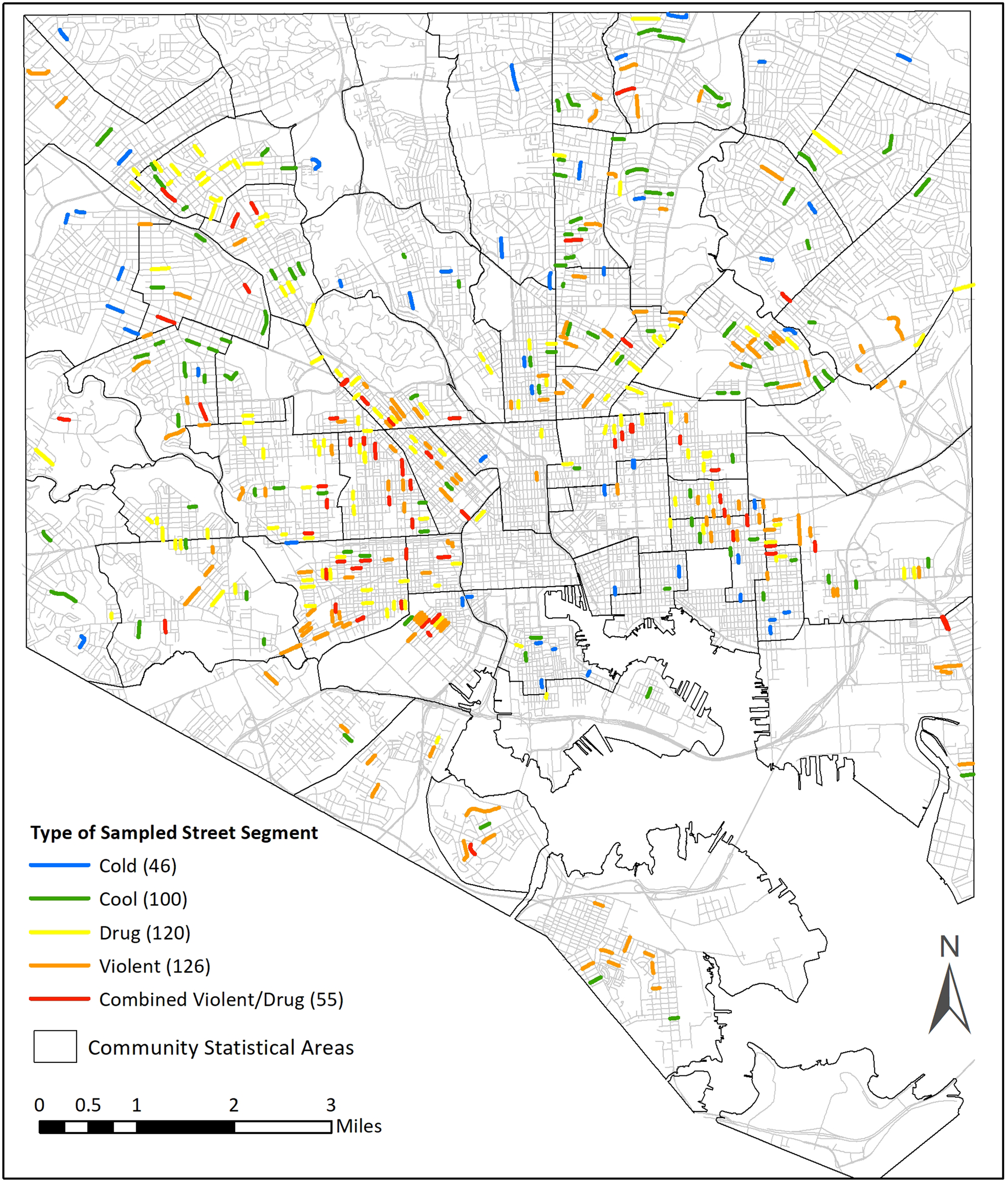
Study sample of street segments by crime type.

We recognize that the over-sampling of crime hot spots leads to a sample of places that includes a much larger number of hot spots than would be included had the study randomly sampled streets from the full population of street segments. At the same time, given our interest in perceptions of policing, the inclusion of large numbers of streets with a strong police presence seems particularly important. Fully 86.4% of the population of residential streets did not meet the criteria for a hot spot, meaning that if the streets had been sampled randomly, only a small number of crime hot spots as we define them would have been included in the sample.

Data Collection

Door-to-door residential surveys and physical observations were conducted from August, 2013 to June, 2014 for the first wave of the study. All baseline estimates are taken from this wave of data collection. Wave 2 data were gained from a survey conducted between April, 2017 and March, 2018.

Residential dwelling units were randomly sampled, and trained field researchers interviewed the first adult resident contacted (21 years or older) who had lived on the street for at least three months.⁶ Respondents were compensated $15 for their participation, and the survey took about 20–25 min to complete. The contact rate for the first wave of the survey was 71.2% and cooperation rate was 60.5%, and for the time 2 wave the contact and cooperation rates were 78.9% and 58%, respectively. These are above average response rates for door-to-door surveying (Babbie 2007; Holbrook, Krosnick, and Pfent 2008).

A total of 3,723 residential surveys were conducted in wave 1, with an average of eight surveys completed on each street, and 3,127 were conducted in the time 2 wave with an average of seven surveys completed on each street. The median number of occupied households on each street was 38 households in both wave 1 and wave 2. At least seven surveys on each street were completed for 98 percent of the sampled streets in wave 1 and 87 percent of the sample in wave 2. As noted earlier, relying on the finite population correction, these samples are equivalent to 9 surveys in wave 1 and about 8 surveys in wave 2 in an infinite population.⁷

Dependent Variable: The “Scorecard” of Procedural Justice and Effectiveness

The citizen survey included items designed to measure general macro-level assessments of PJ and PE on the street on which the respondent lived. All items used a 4-point Likert scale with response options of strongly disagree, disagree, agree, and strongly agree. We used exploratory factor analysis (EFA) with individual survey responses to identify whether the latent structure for these items was consistent with the initial conceptualization that informed the items’ construction using Stata's (Version 16) principal axis factoring procedure (see Table 1). The results suggested a single latent structure that we term the scorecard for citizen perceptions of PJ and PE. We based this on the scree plot, the number of eigenvalues greater than 1, and an examination of the structure for a two-factor solution. Only the first factor had an eigenvalue greater than one. For wave 1, the eigenvalues were: 3.30, 0.10, 0.00, −0.09, −0.10, −0.15. For wave 2, the eigenvalues were: 3.09, 0.07, 0.05, −0.09, −0.13, −0.16. Two-factor solutions for both wave 1 and wave 2 with both orthogonal (Varimax) and oblique (Promax) rotations produced structures that were neither simple (i.e., each item loading on a single factor) nor theoretically meaningful.

Table 1.

Principal Axis Factor Analysis for Scorecard of PJ and PE from Wave 1 and Wave 2.

Item (Eigenvalue)	Factor Loading
Scorecard of PJ and PE – Wave 1 (λ = 3.30)
1. Police officers treat people fairly. (PJ)	0.79
2. In general, the police care about your problems on your block. (PJ)	0.81
3. In general, police officers treat people with respect. (PJ)	0.76
4. In general, the police do a good job preventing crime. (PE)	0.77
5. The police do a good job controlling drug activity. (PE)	0.75
6. The police do a good job enforcing traffic laws. (PE)	0.53
Scorecard of PJ and PE – Wave 2 (λ = 3.09)
1. Police officers treat people fairly. (PJ)	0.73
2. In general, the police care about your problems on your block. (PJ)	0.79
3. In general, police officers treat people with respect. (PJ)	0.78
4. In general, the police do a good job preventing crime. (PE)	0.73
5. The police do a good job controlling drug activity. (PE)	0.73
6. The police do a good job enforcing traffic laws. (PE)	0.51

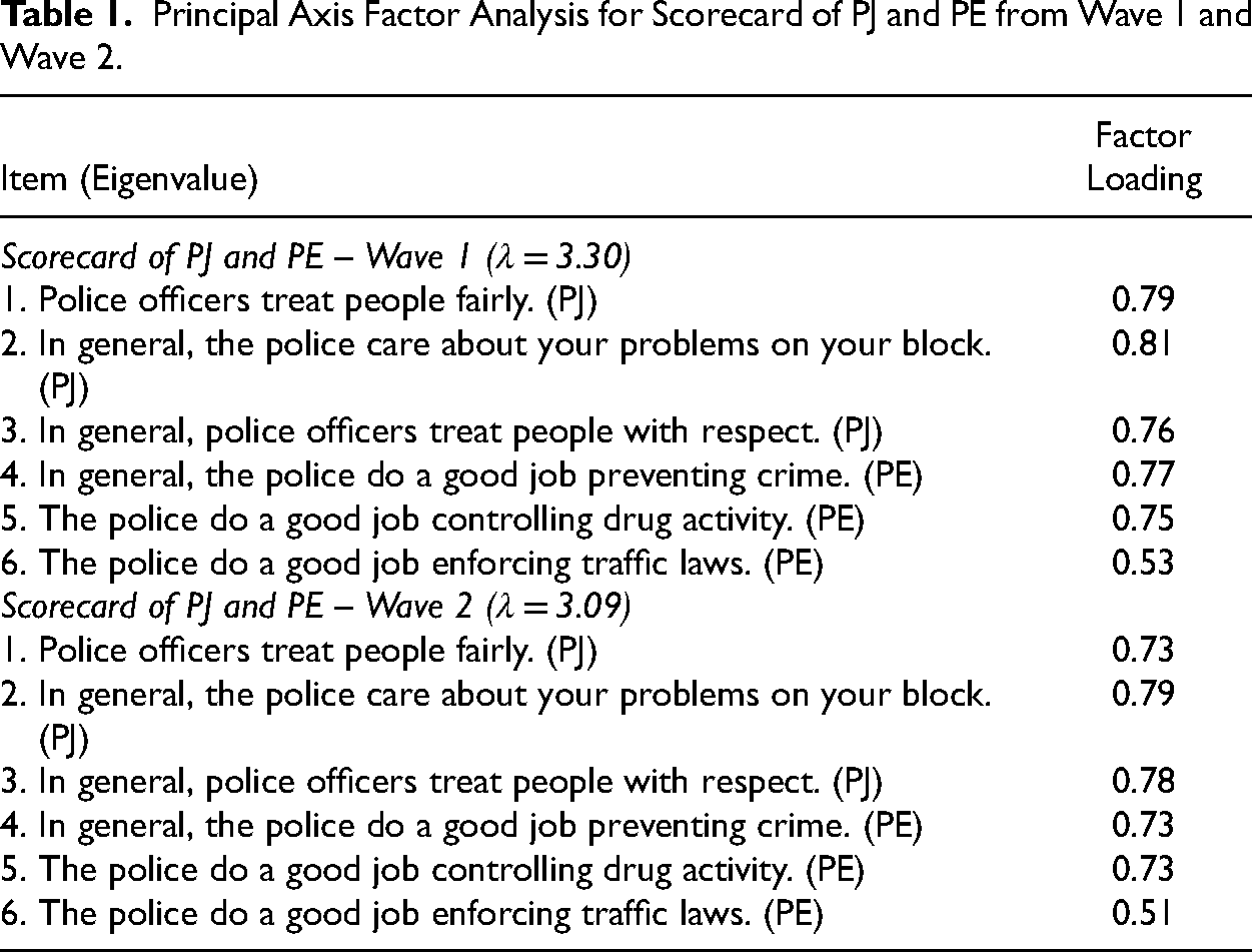
We recognize that PJ and PE are theoretically distinct, and are generally treated by researchers as two separate factors (see review above). At the same time, and as identified by several researchers, in this body of work the conceptual differentiation between constructs is not always supported by statistical analyzes, suggesting that survey respondents may not always fully distinguish between notions such as “fairness” and “effectiveness” (see Gau 2011; Kochel 2013, 2018; Maguire and Johnson 2010; Reisig, Bratton, and Gertz 2007). We thus found it important to ensure the construct and discriminant validity of our scales, and relied on the results of the EFA, which, as already noted, suggest a single latent structure for PJ and PE in this data.

To ensure consistent scaling across waves, our final scorecard measure of public perception of the police is a simple mean of the scores across the six items (α = 0.88 for wave 1; α = .86 for wave 2). These mean scores were highly correlated with factor scores. For wave 1, the correlation was 0.995. For wave 2, the correlation was 0.994. These high correlations reflect the high and similar factor loadings across items for the single factor solution. The individual mean scores were aggregated to create street-level means for our analyzes.

Independent Variables

Following our earlier discussion, we divide the measures into those that reflect experiences with the police, those that reflect conditions on the streets that can be influenced by the police, and those variables that reflect characteristics of the streets that are not within direct influence of the police. We note at the outset that we include the police scorecard estimates for time 1 as an independent variable. This allows us to estimate a residualized difference in differences model, in which our primary concern is what produces change at street segments between wave 1 and wave 2. The independent variables are measured as change variables between wave 1 and wave 2, except in the case of concentrated disadvantage, which is found here (and in prior studies) to be relatively stable across time (Sampson 2009, 2012; Sampson and Morenoff 2006), and mean age and percent female, which are included as demographic control measures from time 1. The use of change variables enables us to examine how changes in these characteristics between waves influenced changes in the scorecard of policing.

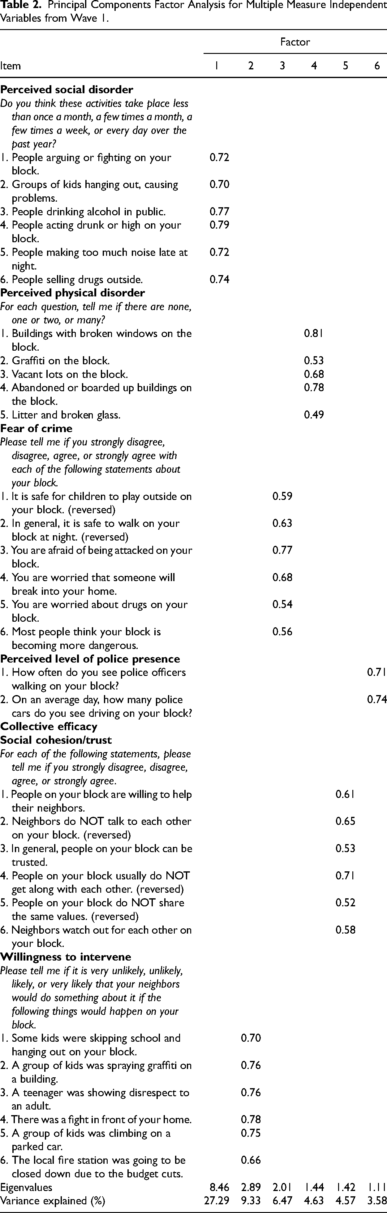
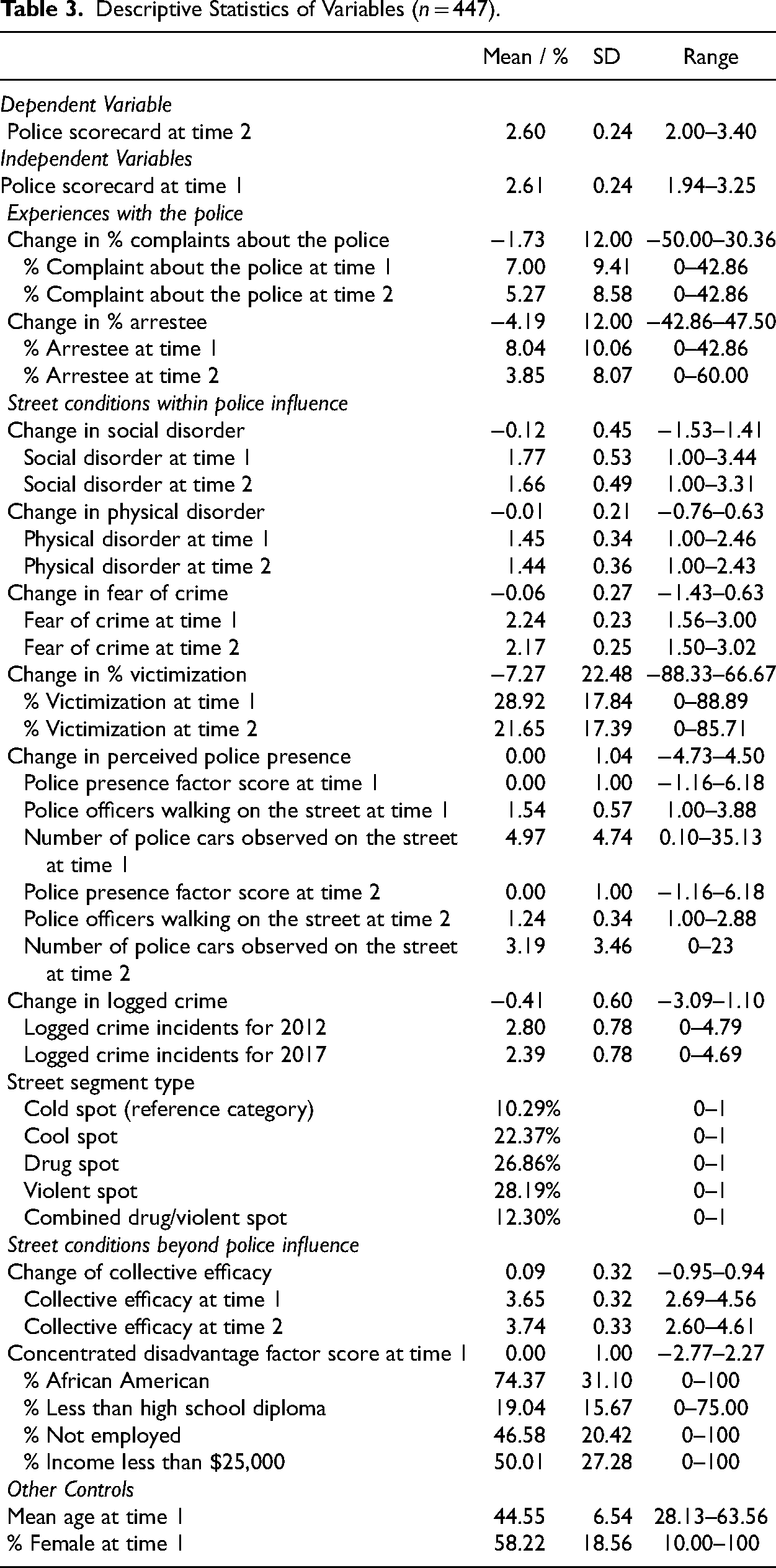
Because we discussed our reasoning for including specific measures earlier, we describe here only the measurement of these variables. Due both to the large number of possible covariates reflecting the theoretical constructs in our model (and the potential for multicollinearity across covariates), and our desire to ensure construct and discriminant validity, we used principal components factor analysis at the individual level to identify composite variables when several street-level variables measured a single theoretical construct (See Table 2 for a full listing of measures included in composite variables). Table 3 provides descriptive statistics of all the variables included in this study.⁸

Table 2.

Principal Components Factor Analysis for Multiple Measure Independent Variables from Wave 1.

	Factor
Item	1	2	3	4	5	6
Perceived social disorder
Do you think these activities take place less than once a month, a few times a month, a few times a week, or every day over the past year?
1. People arguing or fighting on your block.	0.72
2. Groups of kids hanging out, causing problems.	0.70
3. People drinking alcohol in public.	0.77
4. People acting drunk or high on your block.	0.79
5. People making too much noise late at night.	0.72
6. People selling drugs outside.	0.74
Perceived physical disorder
For each question, tell me if there are none, one or two, or many?
1. Buildings with broken windows on the block.				0.81
2. Graffiti on the block.				0.53
3. Vacant lots on the block.				0.68
4. Abandoned or boarded up buildings on the block.				0.78
5. Litter and broken glass.				0.49
Fear of crime
Please tell me if you strongly disagree, disagree, agree, or strongly agree with each of the following statements about your block.
1. It is safe for children to play outside on your block. (reversed)			0.59
2. In general, it is safe to walk on your block at night. (reversed)			0.63
3. You are afraid of being attacked on your block.			0.77
4. You are worried that someone will break into your home.			0.68
5. You are worried about drugs on your block.			0.54
6. Most people think your block is becoming more dangerous.			0.56
Perceived level of police presence
1. How often do you see police officers walking on your block?						0.71
2. On an average day, how many police cars do you see driving on your block?						0.74
Collective efficacy
Social cohesion/trust
For each of the following statements, please tell me if you strongly disagree, disagree, agree, or strongly agree.
1. People on your block are willing to help their neighbors.					0.61
2. Neighbors do NOT talk to each other on your block. (reversed)					0.65
3. In general, people on your block can be trusted.					0.53
4. People on your block usually do NOT get along with each other. (reversed)					0.71
5. People on your block do NOT share the same values. (reversed)					0.52
6. Neighbors watch out for each other on your block.					0.58
Willingness to intervene
Please tell me if it is very unlikely, unlikely, likely, or very likely that your neighbors would do something about it if the following things would happen on your block.
1. Some kids were skipping school and hanging out on your block.		0.70
2. A group of kids was spraying graffiti on a building.		0.76
3. A teenager was showing disrespect to an adult.		0.76
4. There was a fight in front of your home.		0.78
5. A group of kids was climbing on a parked car.		0.75
6. The local fire station was going to be closed down due to the budget cuts.		0.66
Eigenvalues	8.46	2.89	2.01	1.44	1.42	1.11
Variance explained (%)	27.29	9.33	6.47	4.63	4.57	3.58

Table 3.

Descriptive Statistics of Variables (n = 447).

	Mean / %	SD	Range
Dependent Variable
Police scorecard at time 2	2.60	0.24	2.00–3.40
Independent Variables
Police scorecard at time 1	2.61	0.24	1.94–3.25
Experiences with the police
Change in % complaints about the police	−1.73	12.00	−50.00–30.36
% Complaint about the police at time 1	7.00	9.41	0–42.86
% Complaint about the police at time 2	5.27	8.58	0–42.86
Change in % arrestee	−4.19	12.00	−42.86–47.50
% Arrestee at time 1	8.04	10.06	0–42.86
% Arrestee at time 2	3.85	8.07	0–60.00
Street conditions within police influence
Change in social disorder	−0.12	0.45	−1.53–1.41
Social disorder at time 1	1.77	0.53	1.00–3.44
Social disorder at time 2	1.66	0.49	1.00–3.31
Change in physical disorder	−0.01	0.21	−0.76–0.63
Physical disorder at time 1	1.45	0.34	1.00–2.46
Physical disorder at time 2	1.44	0.36	1.00–2.43
Change in fear of crime	−0.06	0.27	−1.43–0.63
Fear of crime at time 1	2.24	0.23	1.56–3.00
Fear of crime at time 2	2.17	0.25	1.50–3.02
Change in % victimization	−7.27	22.48	−88.33–66.67
% Victimization at time 1	28.92	17.84	0–88.89
% Victimization at time 2	21.65	17.39	0–85.71
Change in perceived police presence	0.00	1.04	−4.73–4.50
Police presence factor score at time 1	0.00	1.00	−1.16–6.18
Police officers walking on the street at time 1	1.54	0.57	1.00–3.88
Number of police cars observed on the street at time 1	4.97	4.74	0.10–35.13
Police presence factor score at time 2	0.00	1.00	−1.16–6.18
Police officers walking on the street at time 2	1.24	0.34	1.00–2.88
Number of police cars observed on the street at time 2	3.19	3.46	0–23
Change in logged crime	−0.41	0.60	−3.09–1.10
Logged crime incidents for 2012	2.80	0.78	0–4.79
Logged crime incidents for 2017	2.39	0.78	0–4.69
Street segment type
Cold spot (reference category)	10.29%		0–1
Cool spot	22.37%		0–1
Drug spot	26.86%		0–1
Violent spot	28.19%		0–1
Combined drug/violent spot	12.30%		0–1
Street conditions beyond police influence
Change of collective efficacy	0.09	0.32	−0.95–0.94
Collective efficacy at time 1	3.65	0.32	2.69–4.56
Collective efficacy at time 2	3.74	0.33	2.60–4.61
Concentrated disadvantage factor score at time 1	0.00	1.00	−2.77–2.27
% African American	74.37	31.10	0–100
% Less than high school diploma	19.04	15.67	0–75.00
% Not employed	46.58	20.42	0–100
% Income less than $25,000	50.01	27.28	0–100
Other Controls
Mean age at time 1	44.55	6.54	28.13–63.56
% Female at time 1	58.22	18.56	10.00–100

Experiences with the police

We measure change in complaints about the police focusing on the change in the percent of respondents on the street who “had filed a complaint about the police while living on the block” between the two waves. We also asked the respondents whether they were arrested in the past year, and measured change in the percent of people reported being arrested between the two waves. We recognize that there may be significant measurement error in these two variables because of the relatively low average base rates at the street segment level. At the same time, the variation across segments is quite large, ranging for complaints from −50 to 30 percent, and for arrests from −43 to 47 percent (see Table 3).

Conditions on the streets that can be attributed to the police

We measured change in perceived social disorder by asking respondents a series of questions regarding social disorder on the street. Response options included: every day, a few times a week, a few times a month, or less than once a month. Individual mean scores were created for the 6-item scale (α = 0.88 for wave 1; α = 0.89 for wave 2) that were aggregated to create street-level means. We then subtracted the score at wave 1 from the score at wave 2.

Change in perceived physical disorder was measured using five items in the survey that asked respondents how many physical disorders were present on their street. The questions were measured on a three-point scale consisting of none, one or two, and many. Individual mean scores were created for the 5-item scale (α = 0.74 for wave 1; α = 0.77 for wave 2), then aggregated for street-level means. Again, the means for wave 1 were then subtracted from wave 2.

We measured change in fear of crime using six items.⁹ The questions were measured on a four-point Likert scale ranging from strongly disagree to strongly agree, and referenced the street on which a respondent lived. Individual mean scores were again created for the 6-item scale (α = 0.79 for wave 1; α = 0.81 for wave 2) that were then aggregated for creating street-level means, and then wave 1 scores were subtracted from wave 2 scores.

Change in victimization was measured as the change in the percent of citizens on a street that reported being victimized in the past year in each wave.

Change in police presence was measured as the difference between wave 1 and wave 2 of a factor score developed from two measures asking how often the citizen sees police walking on their street (every day, a few times a week, a few times a month, or less than once a month) and the number of police cars they see driving on their block on an average day (Bradford, Jackson, and Stanko 2009).¹⁰

Change in crime is measured by subtracting the logged crime incidents for the sample selection year of the study (2012) from the logged crime incidents for 2017, the year wave 2 data were primarily collected. Finally, taking the design of the sample into consideration, we also accounted for the street segment type from the original sampling frame, with cold streets serving as the reference category.¹¹

Characteristics of the streets beyond police influence

For change in collective efficacy, wave 1 scores of collective efficacy were subtracted from wave 2 scores. Collective efficacy (Sampson, Raudenbush, and Earls 1997) consists of two scales (each including six items): social cohesion/trust (α = 0.76 for wave 1; α = 0.80 for wave 2), and willingness to intervene (α = 0.86 for wave 1; α = 0.87 for wave 2).¹² Questions were asked about the street on which a person lived. For the collective efficacy measure, individual mean scores were created for each scale, then aggregated to create street-level means, and finally combined to create a single, street-level scale of collective efficacy.

Our concentrated disadvantage measure at the street-segment level consists of percent African American, percent with less than high school diploma, percent not employed, and percent earning an annual income of less than $25,000. The survey provided direct measures of social and economic disadvantage, which we aggregated from individual survey responses from time 1 to the street level (see Weisburd, White, and Wooditch 2020).¹³

We also take into account the mean age of respondents on the street and percent of female respondents at time 1.¹⁴

Analytic Strategy

Mixed effects ordinary least squares (OLS) regression modeling techniques performed in Stata 16 were used to examine the variables that influence the street-level police scorecard in the time 2 survey wave. Because the baseline scorecard is included in the model, the remaining variables are predicting residualized change in the time 2 scorecard. We noted earlier our logic in explaining the police scorecard at the unit of places. However, in order to assess whether using the street-level scorecard is empirically justified, we first estimated a random effects model in which individuals correspond with level 1 in the model, while the street segments serve as the level 2. In the unconditional model, the reported likelihood ratio test for the variance component of the random effects was significant (χ² = 15.87, p < 0.001), indicating significant variation across the street segment means for the scorecard, justifying the use of the street-level scorecard of PJ and PE as the dependent variable. Further statistical support for the analysis of outcomes at the street segment level is gained when we examine the independent variables based on individual perceptions. These variables – social disorder, physical disorder, fear of crime, and collective efficacy – also have significant variability across the street segment means.¹⁵

To take into account the fact that the street segments in each wave are nested within larger communities, we use Community Statistical Areas (CSAs), which are developed by the Baltimore City Department of Planning and Baltimore Data Collaborative. The Collaborative divided the city of Baltimore into 55 CSAs to be consistent with perceived neighborhood boundaries. CSAs are often used for the purpose of social planning and tracking trends in city conditions and demographics, and are commonly used in community research across a number of disciplines (e.g., see Gomez 2016; Merse, Buckley, and Boone 2008; Weisburd, White, and Wooditch 2020). The CSAs are shaded in the map in Figure 1.¹⁶

The full model estimated can be represented as: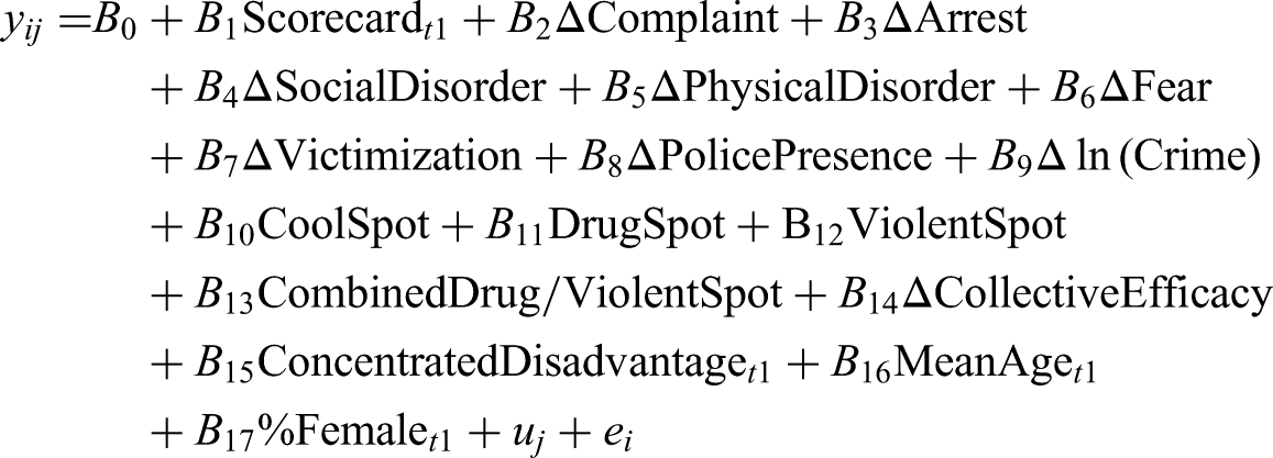

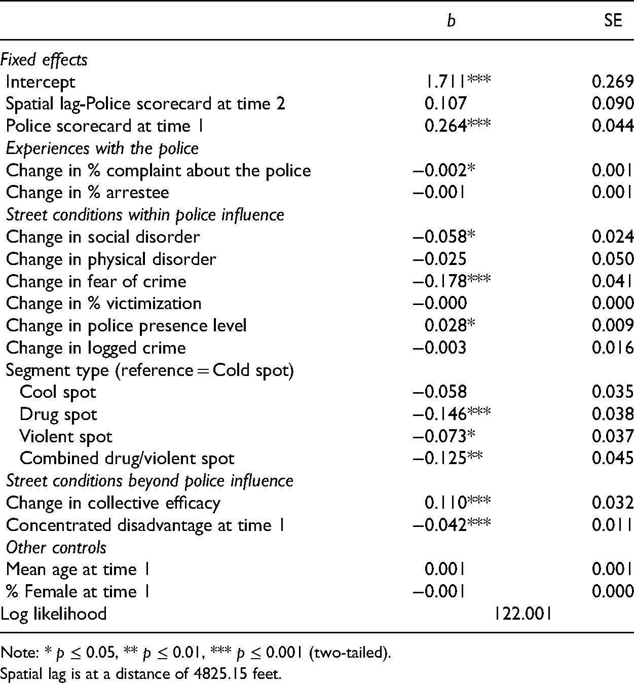
\begin{aligned} y_{i j} = & B_{0} + B_{1} Scorecar d_{t 1} + B_{2} Δ Complaint + B_{3} Δ Arrest \\ + B_{4} Δ SocialDisorder + B_{5} Δ PhysicalDisorder + B_{6} Δ Fear \\ + B_{7} Δ Victimization + B_{8} Δ PolicePresence + B_{9} Δ \ln (Crime) \\ + B_{10} CoolSpot + B_{11} DrugSpot + B_{12} ViolentSpot \\ + B_{13} CombinedDrug / ViolentSpot + B_{14} Δ CollectiveEfficacy \\ + B_{15} ConcentratedDisadvantag e_{t 1} + B_{16} MeanAg e_{t 1} \\ + B_{17} % Femal e_{t 1} + u_{j} + e_{i} \end{aligned}

The intercept is represented by

B_{0}

, and the scorecard at wave 1 by

B_{1} Scorecar d_{t 1}

. The independent variables described above follow with Δ used to represent measures represented as change between wave 1 and wave 2. Finally, we include a random effect (

u_{j}

) for the CSAs to take into account the nesting of streets within communities, and the street-level error term (

e

). In the unconditional model in which street segment and community correspond with level 1 and level 2 respectively, the reported likelihood ratio test for the variance component of the random effects was significant (χ² = 39.17, p < 0.001).

While our hot spot streets were spread through the city widely, and were sampled to be at a minimum one block distant from one another, we also tested for spatial dependence of the dependent variable. Using ArcMap 10.6, we estimated the residuals from the full mixed model and performed Moran's I for spatial autocorrelation. The result (−0.017) was not statistically significant (p = 0.405). In turn, since our sample represents a very small proportion of the streets in the city (1.7%), and the minimum distance for calculating the spatial lag term for the dependent variable is very large (4825.6 feet), we think that the mixed model approach is appropriate. However, as a sensitivity test for our analyzes, we also estimated the models using spatial lag regression in Geoda 12.1. The results follow closely the main models reported below (see Appendix A).

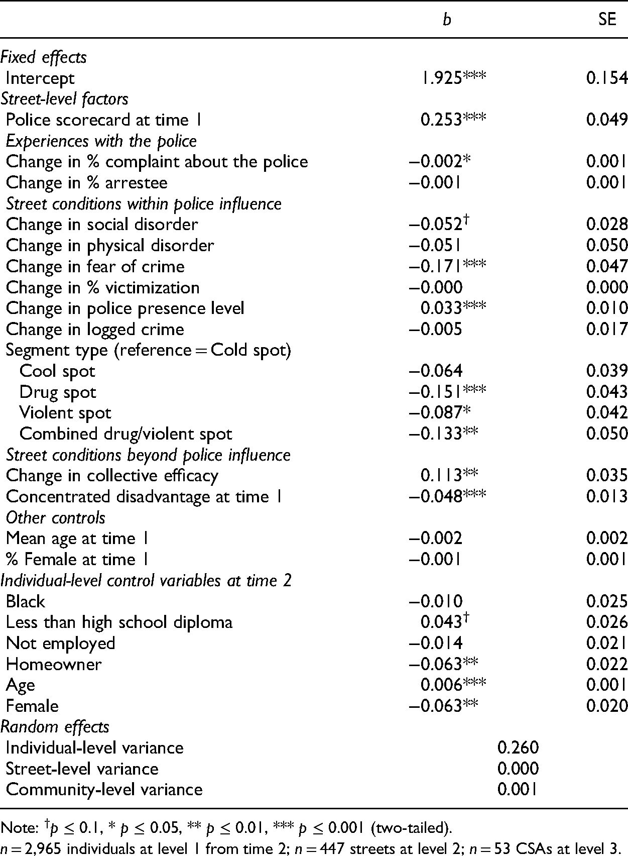
As a sensitivity test, we ran our models predicting individual level scorecard outcomes. While our study was designed as a longitudinal study of street segments and not necessarily of individual change across time, we thought it important to assess whether our findings reflected some type of ecological fallacy, whereby averaging lead to erroneous findings at the street segment level (Robinson 1950). To do this, and to maintain a sufficient sample size, we estimate a three-level multilevel model, where level 3 includes the CSAs, level 2 includes all street-level independent variables, and level 1 includes individual socio-demographic measures (including race, education, home ownership, age and gender) measured at time 2. The main findings of this sensitivity test follow closely those reported in our analyzes at the place level (see Appendix B). We also conducted sensitivity analyzes on independent variables that were time 2 minus time 1 change scores. Instead of using the change score, we ran models that included the time 2 and time 1 variables individually (see Appendix C). Again, the results are generally consistent with our main findings below.¹⁷

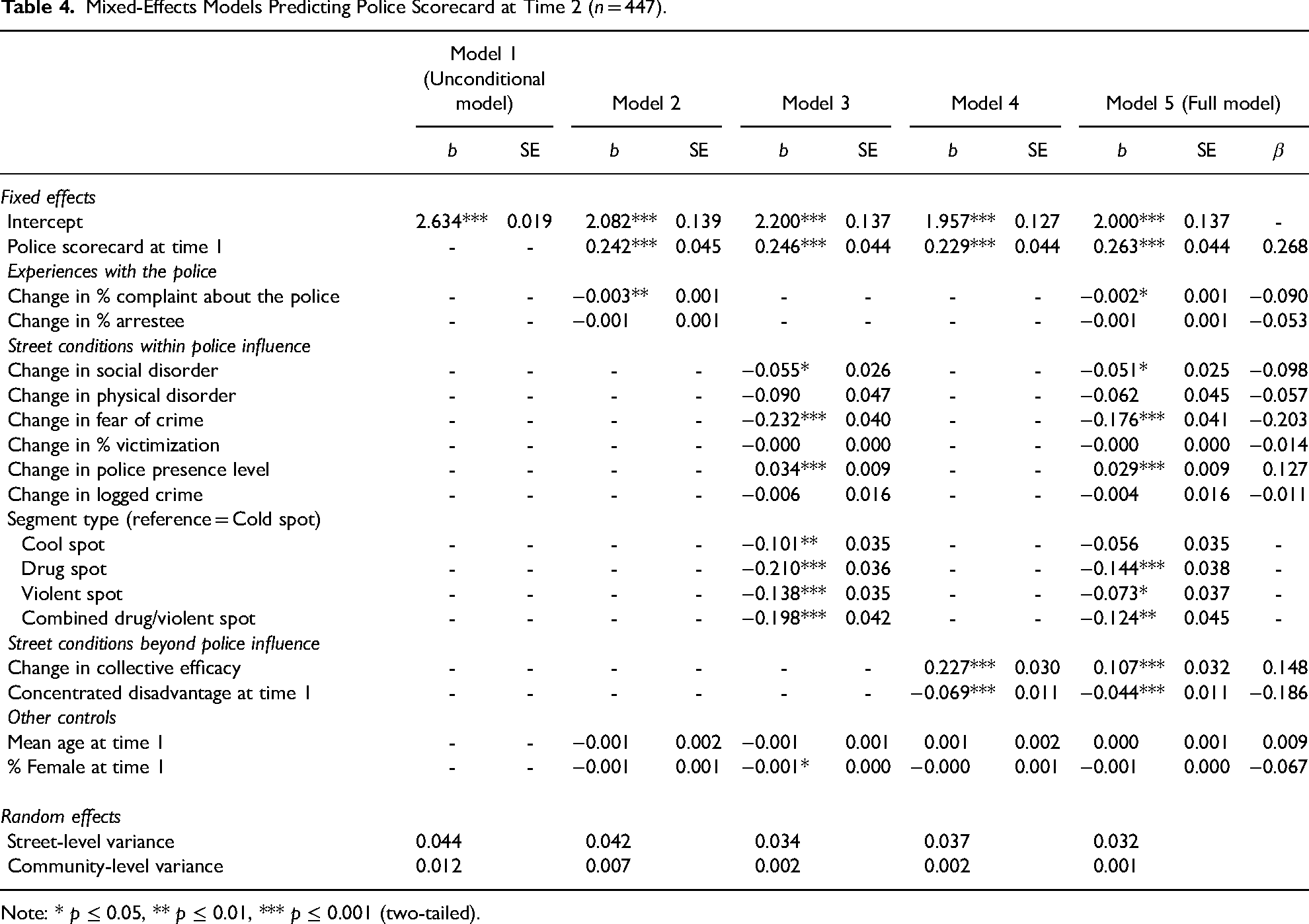
Table 4 reports a series of models. Model 1 is the unconditional model; models 2 thru 4 are the models showing the three sets of variables described above separately. Model 5 represents the full model.¹⁸ In the full model we also report standardized coefficients (β) for the scaled variables to facilitate comparison of coefficients across independent variables.

Table 4.

Mixed-Effects Models Predicting Police Scorecard at Time 2 (n = 447).

	Model 1 (Unconditional model)		Model 2		Model 3		Model 4		Model 5 (Full model)
	b	SE	b	SE	b	SE	b	SE	b	SE	β
Fixed effects
Intercept	2.634***	0.019	2.082***	0.139	2.200***	0.137	1.957***	0.127	2.000***	0.137	-
Police scorecard at time 1	-	-	0.242***	0.045	0.246***	0.044	0.229***	0.044	0.263***	0.044	0.268
Experiences with the police
Change in % complaint about the police	-	-	−0.003**	0.001	-	-	-	-	−0.002*	0.001	−0.090
Change in % arrestee	-	-	−0.001	0.001	-	-	-	-	−0.001	0.001	−0.053
Street conditions within police influence
Change in social disorder	-	-	-	-	−0.055*	0.026	-	-	−0.051*	0.025	−0.098
Change in physical disorder	-	-	-	-	−0.090	0.047	-	-	−0.062	0.045	−0.057
Change in fear of crime	-	-	-	-	−0.232***	0.040	-	-	−0.176***	0.041	−0.203
Change in % victimization	-	-	-	-	−0.000	0.000	-	-	−0.000	0.000	−0.014
Change in police presence level	-	-	-	-	0.034***	0.009	-	-	0.029***	0.009	0.127
Change in logged crime	-	-	-	-	−0.006	0.016	-	-	−0.004	0.016	−0.011
Segment type (reference = Cold spot)
Cool spot	-	-	-	-	−0.101**	0.035	-	-	−0.056	0.035	-
Drug spot	-	-	-	-	−0.210***	0.036	-	-	−0.144***	0.038	-
Violent spot	-	-	-	-	−0.138***	0.035	-	-	−0.073*	0.037	-
Combined drug/violent spot	-	-	-	-	−0.198***	0.042	-	-	−0.124**	0.045	-
Street conditions beyond police influence
Change in collective efficacy	-	-	-	-	-	-	0.227***	0.030	0.107***	0.032	0.148
Concentrated disadvantage at time 1	-	-	-	-	-	-	−0.069***	0.011	−0.044***	0.011	−0.186
Other controls
Mean age at time 1	-	-	−0.001	0.002	−0.001	0.001	0.001	0.002	0.000	0.001	0.009
% Female at time 1	-	-	−0.001	0.001	−0.001*	0.000	−0.000	0.001	−0.001	0.000	−0.067

Random effects
Street-level variance	0.044		0.042		0.034		0.037		0.032
Community-level variance	0.012		0.007		0.002		0.002		0.001

Note: * p ≤ 0.05, ** p ≤ 0.01, *** p ≤ 0.001 (two-tailed).

Findings

Reflecting the relative stability of attitudes toward the scorecard on street segments, the scorecard in wave 1 has the strongest impact of any of the independent variables on the scorecard at wave 2 (β = 0.27, p < 0.001).

Looking at our measures of experiences with the police, we find that when there is an increase in the proportion of complaints, there is a significant decrease in the scorecard, though this effect is modest (β = −0.09, p < 0.05). Change in the percent of people reported being arrested is not statistically associated with the scorecard at wave 2, though it is in the expected direction (p = 0.168).

Several of the measures that reflect street conditions over which the police can presumably have influence have statistically significant impacts on the scorecard. The largest effect is produced by fear of crime (β = −0.20, p < 0.001). Increases in perceived social disorder also led to a decrease in the scorecard (β = −0.10, p < 0.05) and increases in police presence led to increases in street-level evaluations of the scorecard (β = 0.13, p < 0.001). Change in victimization does not significantly impact upon the scorecard. Street segment type has an overall statistically significant impact on the scorecard (p < 0.001),¹⁹ with the impact of the drug hot spots, violent hot spots, and combined drug/violent crime hot spots particularly associated with low scorecard values. Change in crime, however, is not a statistically significant variable in the model.²⁰

While many of the measures that reflect experiences with the police, or conditions the police may reasonably be seen to impact, are significantly related to the scorecard, our model also shows important influences for variables that are likely to be primarily influenced by forces outside of police influence. Concentrated disadvantage has the third largest standardized score (β = −0.19) in the model, with higher levels of concentrated disadvantage significantly associated with lower scorecard values in wave 2 (p < 0.001). Change in collective efficacy has a slightly smaller standardized effect (β = 0.15) and is also highly significant (p < 0.001), with increasing levels of collective efficacy associated with higher scorecard values. Finally, neither of our demographic control variables are statistically significant in the full model.

Looking at models 2–4, we can see that the three dimensions we examine remain relatively stable in terms of their influences, whether they are examined individually or within the larger model. All the significant measures when measuring a domain individually remain statistically significant in the overall model, and the measures that are not statistically significant do not attain statistical significance in the full model.

Discussion

Scorecard values in wave 1 of our survey were strongly predictive of scorecard values in wave 2. This finding suggests that average place-level evaluations of PJ and PE are to some degree stable traits. This supports scholars that emphasize the degree to which such values are, in large part, determined historically and not simply by the immediate situational features of police behavior or social or environmental changes (Nagin and Telep 2017; White, Weisburd, and Wire 2018). At the same time, our study points to a number of more immediate changes at the street-segment level that do influence average evaluations of PJ and PE across places, measured as a scorecard of policing in our study.

We find evidence that some experiences with the police (those leading to formal complaints) have an effect on average place-level evaluations of the scorecard. Our model assumed that the impacts of such variables would be both direct and vicarious. When someone has a bad experience with the police and files a complaint, we made the assumption that this may also be communicated to one's immediate neighbors, who share those similar experiences. Our findings suggest that this may be the case, with increasing levels of complaints between the two waves of the survey leading to decreasing PJ/PE scores at the street level. This finding follows other research that identifies negative encounters with the police as particularly important in forming opinions about the police (e.g. Skogan 2006). At the same time, the percent of people who had been arrested does not significantly affect the scorecard. This might be the case because arrests are often neither visible (i.e., when taking place inside a private dwelling) nor discussed openly due to a sense of shame. At the same time, we should note that the effect of change in percent of arrestees on the street is in the expected direction, even though it did not achieve statistical significance. In a larger sample arrests might have emerged as a significant antecedent of PJ and PE.

Factors that can be seen as potentially within police influence but not necessarily part of the immediate experience of citizens with the police, were found to be strongly related to the scorecard in wave 2. Increased perceived police presence, increased levels of fear at the street segments, and increases in social disorder, all significantly influenced the scorecard values. We suspect that this is part of the “accountability mechanism” noted earlier. When local residents are less fearful, see more police around, or perceive social disorder as reduced, they may naturally give credit (or at least partial credit) to the police, which, in turn, impacts shared views of the scorecard of policing. Our analyses show this outcome at a collective level, reflecting average changes in perceptions of people who live on a street.

It is interesting in this regard that we do not find that changes in objective levels of crime (at least as measured by the police) influence the scorecard of PJ and PE, while our sampling categories of hot spots do have an impact. One reason for this may be that citizens do not look at crime numbers, but rather at what they see as the safety or security of their streets. While marginal changes in crime may not be very visible to people who live on a street, living on a street that was defined as a hot spot in our study was likely to be easily observable. We also do not find significant impacts for physical disorder. We think this finding is consistent with Robert Sampson’s (2012) observation that the meaning of physical disorder may vary community to community, or in our case street to street, with people on different streets viewing street-level physical disorder as less or more serious.

Our model points to the strong impact of measures primarily outside of police influence in forming general evaluations of police fairness and effectiveness at the street segment. Increases in average place levels of collective efficacy and lower concentrated disadvantage lead to increased levels of the scorecard of PJ and PE. These findings are consistent with a large body of research reviewed earlier that shows a positive relationship between collective efficacy and satisfaction with the police (e.g., Bradford and Myhill 2015; Kochel 2012; Nix et al. 2015, Sargeant, Wickes, and Mazerolle 2013), and concentrated disadvantage and negative attitudes toward the police (Apple and O’Brien 1983; Dunham and Alpert 1988; Reisig and Parks 2000; Sampson, Raudenbush, and Earls 1997; Weitzer 1999; Wu, Sun, and Triplett 2009). At the same time, they provide new insight into how general street-level evaluations of police fairness and effectiveness are formed. Our findings suggest that street-level perceptions are also strongly influenced by factors not directly influenced by standard models of policing. This is in line with recent findings by Pickett, Nix, and Roche (2018), which show that more general relationships, such as teacher- or parent-provided PJ may, over time and through a relational justice schema, impact perceptions of police-provided PJ. General assessments of police fairness and effectiveness in this context are only partially determined by the police.

These findings raise important questions about the meaning of street-level attitudes toward the police and the way they should be interpreted by researchers, policy makers, and practitioners. Our analyses suggest that there is significant variability across micro communities (such as street segments) in attitudes toward the police, and we suspect towards criminal justice institutions more generally. Just like assessing citizen attitudes across neighborhoods, communities, and cities is an important focus for scholars, explaining variability at the micro-geographic level should become a more prominent area of research. Our study is the first that we are aware of to take this approach in terms of PJ and PE, but there is growing awareness of the importance of considering collective or group-level PJ (Jonathan-Zamir, Perry, and Weisburd 2021; O’Brien, Tyler, and Meares 2020).

Both the research and policy-oriented literature often view the police as largely responsible for their public image (e.g., President’s Task Force on 21^st Century Policing 2015; Reisig and Parks 2000; Rosenbaum et al. 2005; Skogan 2009; Tyler 2004, 2009; Weitzer and Tuch 2006). Thus, the police may be criticized if public evaluations of their effectiveness or fairness have deteriorated, or praised if citizens view them more positively. Our data suggest, however, that average place-based perceptions of police conduct should be interpreted with caution, recognizing that such perceptions may be rooted, to varying degrees, in factors outside the influence of the police. Police practitioners must recognize that the micro geographies that have become the focus of many proactive policing strategies are affected not simply by what they do at these places, but also by the average social and demographic characteristics of places. In a world in which housing is highly stratified by race and class (reflected by our measure of concentrated disadvantage), historical features of places play a key role in understanding their assessments of how the police behave and how effective they are. This is not a new observation (e.g., Cao, Frank, and Cullen 1996; Sampson and Bartusch 1998; Skogan 2009), but it is reinforced by our study findings.

We think that our study has provided new evidence about the mechanisms underlying place- based evaluations of police fairness and effectiveness. At the same time, we want to note some specific limitations of our study before concluding. While we have a rich dataset to draw from, we were not able to fully measure the nature of experiences of citizens with police at the street-segment level. Complaints and arrests provide proxies for negative experiences. We do not have proxies for positive experiences. More generally, it would clearly be valuable to have observations of encounters with the police in future studies at the place level. In turn, our focus on a sample weighted towards crime hot spots has an advantage of focusing on places where police/citizen interactions are common. However, it may be the case that somewhat different relationships would be observed in a sample weighted toward low crime streets. Finally, despite our attempts to account for change over time, we recognize that our study, like other observational studies, is limited in the causal conclusions that can be reached.

Conclusions

Police scholars and policy makers have placed much emphasis on the ability of the police to influence general assessments of police fairness and effectiveness, and by influencing these attitudes – the overall perceived legitimacy of policing. Despite the strong acceptance of this model, there has been little examination of how the main antecedents of police legitimacy – perceptions of PJ and PE – are formed, particularly at the micro place level, and whether the police can influence such perceptions. Our study focused on these perceptions at the local level of street segments, where interactions between neighbors are likely to be most pronounced, and where policing is often focused. We find support for a model of PJ and PE that recognizes that the police can impact street-level perceptions. Yet, we also find that key antecedents of general evaluations of police fairness and effectiveness at the street level are typically outside the influence of the police. In particular, collective efficacy and concentrated disadvantage play an important role in producing street-level perceptions.

Footnotes

Acknowledgments

We would like to thank Justin Ready, Brian Lawton and Amelia Haviland for their help in conceptualizing the project, and Breanne Cave, Matthew Nelson, Sean Wire, and Victoria Goldberg for their work in supporting data collection.

Declaration of Conflicting Interests

The author(s) declared no potential conflicts of interest with respect to the research, authorship, and/or publication of this article.

Funding

The author(s) disclosed receipt of the following financial support for the research, authorship, and/or publication of this article: This work was supported by the National Institue on Drug Abuse, (grant number R01DA032639). The content is solely the responsibility of the authors and does not necessarily represent the official views of the National Institute on Drug Abuse or NIH.

ORCID iDs

David Weisburd

Tal Jonathan-Zamir

Clair White

Kiseong Kuen

Notes

Author Biographies

David Weisburd is Distinguished Professor of Criminology, Law and Society at George Mason University and Walter E. Meyer Professor of Law and Criminal Justice at the Hebrew University. He is also co-founder and Executive Director of the Center for Evidence Based Crime Policy. Professor Weisburd is well known for his research on policing and crime hot spots. He has received many international prizes including the Stockholm Prize in Criminology (2010), the Sutherland (2014) and Vollmer Awards (2017) from the American Society of Criminology, the Israel Prize (2015), and the Rothschild Prize (2022) in Social Sciences.

Tal Jonathan-Zamir is a Senior Lecturer at the Institute of Criminology, Faculty of Law, the Hebrew University of Jerusalem. Her research focuses on policing, particularly police-community relations, police legitimacy and procedural justice from various perspectives, and more recently – the effects of the COVID-19 pandemic on police-community relations in Israel. Her research has been published in a number of journals including Justice Quarterly, Criminal Justice and Behavior, Law & Society Review, British Journal of Criminology, and Policing: A Journal of Policy & Practice.

Clair White is an Assistant Professor at the University of Wyoming. Her research interests include crime and place/communities, policing, and the criminal justice system's response to mental health problems. Currently her work focuses on police responses to mental health crisis calls, as well as other public health issues and social problems at crime hot spots. Her research has been published in a number of journals including Prevention Science, British Journal of Criminology, American Journal of Preventive Medicine, Criminology & Public Policy, Policing: A Journal of Policy & Practice, and American Journal of Community Psychology.

David B. Wilson is a professor of criminology, law, and society at George Mason University. His research interests focus on the effectiveness of juvenile and offender rehabilitation and crime prevention efforts, program evaluation methodology, and meta-analysis. He was awarded the Marcia Guttentag Award for Early Promise as an Evaluator by the American Evaluation Association in 1999 and the Frederick Mosteller Award for Distinctive Contributions to Systematic Reviewing and in 2021 appointed as a Fellow of the American Society of Criminology.

Kiseong Kuen is a doctoral student in the Department of Criminology, Law and Society at George Mason University and research assistant for the Center for Evidence-Based Crime Policy. His research interests include policing, police legitimacy, crime and place, social problems at crime hot spots, and evidence-based crime policy.

Appendix A. Maximum likelihood spatial lag model predicting police scorecard at time 2

	b	SE
Fixed effects
Intercept	1.711***	0.269
Spatial lag-Police scorecard at time 2	0.107	0.090
Police scorecard at time 1	0.264***	0.044
Experiences with the police
Change in % complaint about the police	−0.002*	0.001
Change in % arrestee	−0.001	0.001
Street conditions within police influence
Change in social disorder	−0.058*	0.024
Change in physical disorder	−0.025	0.050
Change in fear of crime	−0.178***	0.041
Change in % victimization	−0.000	0.000
Change in police presence level	0.028*	0.009
Change in logged crime	−0.003	0.016
Segment type (reference = Cold spot)
Cool spot	−0.058	0.035
Drug spot	−0.146***	0.038
Violent spot	−0.073*	0.037
Combined drug/violent spot	−0.125**	0.045
Street conditions beyond police influence
Change in collective efficacy	0.110***	0.032
Concentrated disadvantage at time 1	−0.042***	0.011
Other controls
Mean age at time 1	0.001	0.001
% Female at time 1	−0.001	0.000
Log likelihood	122.001

Note: * p ≤ 0.05, ** p ≤ 0.01, *** p ≤ 0.001 (two-tailed).

Spatial lag is at a distance of 4825.15 feet.

Appendix B. Mixed-effects models predicting individual-level police scorecard at time 2

	b	SE
Fixed effects
Intercept	1.925***	0.154
Street-level factors
Police scorecard at time 1	0.253***	0.049
Experiences with the police
Change in % complaint about the police	−0.002*	0.001
Change in % arrestee	−0.001	0.001
Street conditions within police influence
Change in social disorder	−0.052^†	0.028
Change in physical disorder	−0.051	0.050
Change in fear of crime	−0.171***	0.047
Change in % victimization	−0.000	0.000
Change in police presence level	0.033***	0.010
Change in logged crime	−0.005	0.017
Segment type (reference = Cold spot)
Cool spot	−0.064	0.039
Drug spot	−0.151***	0.043
Violent spot	−0.087*	0.042
Combined drug/violent spot	−0.133**	0.050
Street conditions beyond police influence
Change in collective efficacy	0.113**	0.035
Concentrated disadvantage at time 1	−0.048***	0.013
Other controls
Mean age at time 1	−0.002	0.002
% Female at time 1	−0.001	0.001
Individual-level control variables at time 2
Black	−0.010	0.025
Less than high school diploma	0.043^†	0.026
Not employed	−0.014	0.021
Homeowner	−0.063**	0.022
Age	0.006***	0.001
Female	−0.063**	0.020
Random effects
Individual-level variance	0.260
Street-level variance	0.000
Community-level variance	0.001

Note: ^†p ≤ 0.1, * p ≤ 0.05, ** p ≤ 0.01, *** p ≤ 0.001 (two-tailed).

n = 2,965 individuals at level 1 from time 2; n = 447 streets at level 2; n = 53 CSAs at level 3.

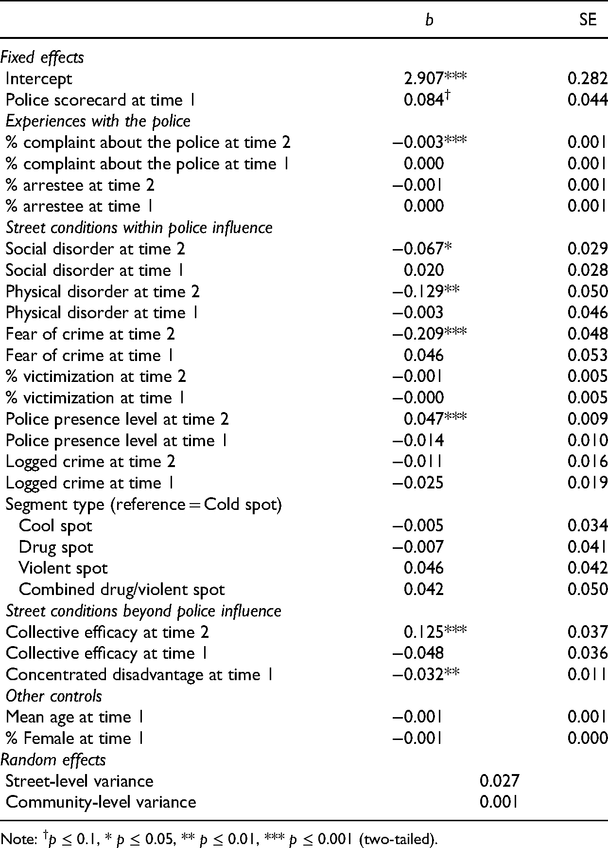
Appendix C. Mixed-effects models using time 1 and time 2 variables instead of change variables

	b	SE
Fixed effects
Intercept	2.907***	0.282
Police scorecard at time 1	0.084^†	0.044
Experiences with the police
% complaint about the police at time 2	−0.003***	0.001
% complaint about the police at time 1	0.000	0.001
% arrestee at time 2	−0.001	0.001
% arrestee at time 1	0.000	0.001
Street conditions within police influence
Social disorder at time 2	−0.067*	0.029
Social disorder at time 1	0.020	0.028
Physical disorder at time 2	−0.129**	0.050
Physical disorder at time 1	−0.003	0.046
Fear of crime at time 2	−0.209***	0.048
Fear of crime at time 1	0.046	0.053
% victimization at time 2	−0.001	0.005
% victimization at time 1	−0.000	0.005
Police presence level at time 2	0.047***	0.009
Police presence level at time 1	−0.014	0.010
Logged crime at time 2	−0.011	0.016
Logged crime at time 1	−0.025	0.019
Segment type (reference = Cold spot)
Cool spot	−0.005	0.034
Drug spot	−0.007	0.041
Violent spot	0.046	0.042
Combined drug/violent spot	0.042	0.050
Street conditions beyond police influence
Collective efficacy at time 2	0.125***	0.037
Collective efficacy at time 1	−0.048	0.036
Concentrated disadvantage at time 1	−0.032**	0.011
Other controls
Mean age at time 1	−0.001	0.001
% Female at time 1	−0.001	0.000
Random effects
Street-level variance	0.027
Community-level variance	0.001

Note: ^†p ≤ 0.1, * p ≤ 0.05, ** p ≤ 0.01, *** p ≤ 0.001 (two-tailed).

References

Alward

L. M.

Baker

. 2021. “Justice-involved Males’ Procedural Justice Perceptions of the Police and Courts: Examining the Spill-Over Effect.” Criminal Justice Studies 34(1):33-47.

Apple

O’Brien

. 1983. “Neighborhood Racial Composition and Residents’ Evaluation of Police Performance.” Journal of Police Science and Administration 11(1):76-84.

Armstrong

T. A.

Katz

C. M.

Schnebly

S. M.

. 2015. “The Relationship Between Citizen Perception of Collective Efficacy and Neighborhood Violent Crime.” Crime and Delinquency 61(1):121-42. https://doi.org/10.1177/0011128710386202

Augustyn

M. B.

2016. “Updating Perceptions of (in)Justice.” Journal of Research in Crime and Delinquency 53(2):255-86.

Babbie

Earl R.

2007. The Practice of Social Research. 11th ed. Belmont: Wadsworth.

Barragan

Sherman

Reiter

Tita

G. E.

. 2016. ““Damned if you do, Damned if you Don’t”: Perceptions of Guns, Safety, and Legitimacy among Detained gun Offenders.” Criminal Justice and Behavior 43(1):140-55.

Bradford

Jackson

Stanko

E. A.

. 2009. “Contact and Confidence: Revisiting the Impact of Public Encounters with the Police.” Policing and Society 19(1):20-46.

Bradford

Myhill

. 2015. “Triggers of Change to Public Confidence in the Police and Criminal Justice System: Findings from the Crime Survey for England and Wales Panel Experiment.” Criminology and Criminal Justice 15(1):23-43.

Braga

A. A.

Papachristos

A. V.

Hureau

D. M.

. 2014a. “The Effects of hot Spots Policing on Crime: An Updated Systematic Review and Meta-Analysis.” Justice Quarterly 31(4):633-63.

10.

Braga

A. A.

Winship

Tyler

T. R.

Fagan

Meares

T. L.

. 2014b. “The Salience of Social Contextual Factors in Appraisals of Police Interactions with Citizens: A Randomized Factorial Experiment.” Journal of Quantitative Criminology 30(4):599-627.

11.

Brick

B. T.

Taylor

T. J.

Esbensen

F. A.

. 2009. “Juvenile Attitudes Towards the Police: The Importance of Subcultural Involvement and Community Ties.” Journal of Criminal Justice 37(5):488-95.

12.

Bridenball

Jesilow

. 2008. “What Matters: The Formation of Attitudes Toward the Police.” Police Quarterly 11(2):151-81.

13.

Brown

Benedict

. 2002. “Perceptions of the Police: Past Findings, Methodological Issues, Conceptual Issues and Policy Implications.” Policing: An International Journal of Police Strategies and Management 25:543-80.

14.

Brunson

R. K.

2007. ““Police Don’t Like Black People”: African-American Young Men’s Accumulated Police Experiences.” Criminology and Public Policy 6(1):71-101.

15.

Brunton-Smith

Jackson

Sutherland

. 2014. “Bridging Structure and Perception: On the Neighbourhood Ecology of Beliefs and Worries About Violent Crime.” The British Journal of Criminology 54(4):503-26.

16.

Cao

Frank

Cullen

F. T.

. 1996. “Race, Community Context, and Confidence in the Police.” American Journal of Police 15(1):3-22.

17.

Cao

. 2019. “Confidence in the Police by Race: Taking Stock and Charting new Directions.” Police Practice and Research 20(1):3-17.

18.

Carr

P. J.

Napolitano

Keating

. 2007. “We Never Call the Cops and Here is why: A Qualitative Examination of Legal Cynicism in Three Philadelphia Neighborhoods.” Criminology; An Interdisciplinary Journal 45(2):445-78.

19.

City Data. 2012. Crime in Baltimore, available online at http://www.city-data.com/crime/crime-Baltimore-Maryland.html (accessed 13 December 2017).

20.

Correia

M. E.

Reisig

M. D.

Lovrich

N. P.

. 1996. “Public Perceptions of State Police: An Analysis of Individual-Level and Contextual Variables.” Journal of Criminal Justice 24(1):17-28.

21.

Covington

Taylor

R. B.

. 1991. “Fear of Crime in Urban Residential Neighborhoods: Implications of Between-and Within-Neighborhood Sources for Current Models.” The Sociological Quarterly 32(2):231-49.

22.

Dai

Time

. 2019. “Understanding Public Satisfaction with the Police: Military Background and Interactions Between Higher Education and Prior Contact with the Police.” Policing: An International Journal 42(4):571-84.

23.

Dai

Johnson

R. R.

. 2009. “Is Neighborhood Context a Confounder?” Policing: An International Journal of Police Strategies and Management 32(4):595-612.

24.

Decker

S. H.

1981. “Citizen Attitudes Toward the Police: A Review of Past Findings and Suggestions for Future Policy.” Journal of Police Science and Administration 9(1):80-7.

25.

Dowler

Sparks

. 2008. “Victimization, Contact with Police, and Neighborhood Conditions: Reconsidering African American and Hispanic Attitudes Toward the Police.” Police Practice and Research: An International Journal 9(5):395-415.

26.

Dunham

R. G.

Alpert

G. P.

. 1988. “Neighborhood Differences in Attitudes Toward Policing: Evidence for a Mixed-Strategy Model of Policing in a Multi-Ethnic Setting.” The Journal of Criminal Law and Criminology 79(2):504-23.

27.

Durkheim

2014. The Division of Labor in Society. New York: Free Press.

28.

Elliott

Thomas

S. D.

Ogloff

J. R.

. 2011. ““Procedural Justice in Contacts with the Police: Testing a Relational Model of Authority in a Mixed Methods Study.” Psychology.” Public Policy, and Law 17(4):592-610.

29.

Ferraro

K. F.

LaGrange

R. L.

. 1987. “The Measurement of Fear of Crime.” Sociological Inquiry 57(1):70-97.

30.

Gau

J. M.

2011. “The Convergent and Discriminant Validity of Procedural Justice and Police Legitimacy: An Empirical Test of Core Theoretical Propositions.” Journal of Criminal Justice 39(6):489-98.

31.

Gau

J. M.

Brunson

R. K.

. 2010. “Procedural Justice and Order Maintenance Policing: A Study of Inner-City Young Men’s Perceptions of Police Legitimacy.” Justice Quarterly 27(2):255-79.

32.

Gau

J. M.

Corsaro

Stewart

E. A.

Brunson

R. K.

. 2012. “Examining Macro-Level Impacts on Procedural Justice and Police Legitimacy.” Journal of Criminal Justice 40(4):333-43.

33.

Gomez

M. B.

2016. “Policing, Community Fragmentation, and Public Health: Observations from Baltimore.” Journal of Urban Health 93:154-67. https://doi.org/10.1007/s11524-015-0022-9

34.

Haberman

C. P.

Groff

E. R.

Ratcliffe

J. H.

Sorg

E. T.

. 2016. “Satisfaction with Police in Violent Crime hot Spots: Using Community Surveys as a Guide for Selecting hot Spots Policing Tactics.” Crime and Delinquency 62(4):525-57.

35.

Hawdon

Ryan

. 2003. “Police-resident Interactions and Satisfaction with Police: An Empirical Test of Community Policing Assertions.” Criminal Justice Policy Review 14(1):55-74.

36.

Hinds

Murphy

. 2007. “Public Satisfaction with Police: Using Procedural Justice to Improve Police Legitimacy.” Australian and New Zealand Journal of Criminology 40(1):27-42.

37.

Hinkle

J. C.

2015. “Emotional Fear of Crime vs. Perceived Safety and Risk: Implications for Measuring “Fear” and Testing the Broken Windows Thesis.” American Journal of Criminal Justice 40(1):147-68. https://doi.org/10.1007/s12103-014-9243-9

38.

Hinkle

J. C.

Yang

S. M.

. 2014. “A new Look into Broken Windows: What Shapes Individuals’ Perceptions of Social Disorder?” Journal of Criminal Justice 42(1):26-35.

39.

Hohl

Bradford

Stanko

E. A.

. 2010. “Influencing Trust and Confidence in the London Metropolitan Police: Results from an Experiment Testing the Effect of Leaflet Drops on Public Opinion.” The British Journal of Criminology 50(3):491-513.

40.

Holbrook

A. L.

Krosnick

J. A.

Pfent

. 2008 “The Causes and Consequences of Response Rates in Surveys by the News Media and Government Contractor Survey Research Firms.” Pp. 449-528 in Advances in Telephone Survey Methodology, edited by Lepkowski

J. M.

Tucker

Brick

M. J.

Leeuw

E. D.

Japec

Lavrakas

P. J.

Link

M. W.

Sangster

R. L.

. New York: Wiley.

41.

Homant

R. J.

Kennedy

D. B.

Fleming

R. M.

. 1984. “The Effect of Victimization and the Police Response on Citizen’s Attitudes Toward Police.” Journal of Police Science and Administration 12:323-32.

42.

Jackson

Bradford

. 2009. “Crime, Policing and Social Order: On the Expressive Nature of Public Confidence in Policing.” The British Journal of Sociology 60:493-521.

43.

Jackson

Bradford

Hohl

Farrall

. 2009. “Does the Fear of Crime Erode Public Confidence in Policing?” Policing: A Journal of Policy and Practice 3(1):100-11.

44.

Jackson

Tyler

T. R.

Hough

Bradford

Mentovich

. 2015 “Compliance and Legal Authority.” Pp. 456-62 in International Encyclopedia of the Social and Behavioral Sciences edited by Wright

J. D.

. Oxford: Elsevier.

45.

Jonathan-Zamir

Perry

Weisburd

. 2021. “Illuminating the Concept of Community (Group)-Level Procedural Justice: A Qualitative Analysis of Protestors’ Group-Level Experiences with the Police.” Criminal Justice and Behavior 48(6):791-809.

46.

Jonathan-Zamir

Weisburd

. 2013. “The Effects of Security Threats on Antecedents of Police Legitimacy: Findings from a Quasi-Experiment in Israel.” Journal of Research in Crime and Delinquency 50(1):3-32.

47.

Kochel

T. R.

2012. “Can Police Legitimacy Promote Collective Efficacy?” Justice Quarterly 29(3):384-419.

48.

Kochel

T. R.

2013. “Robustness of Collective Efficacy on Crime in a Developing Nation: Association with Crime Reduction Compared to Police Services.” Journal of Crime and Justice 36(3):334-52.

49.

Kochel

T. R.

2018. “Police Legitimacy and Resident Cooperation in Crime Hotspots: Effects of Victimisation Risk and Collective Efficacy.” Policing and Society 28(3):251-70.

50.

Kochel

T. R.

Park

Mastrofski

S. R.

. 2013. “Examining Police Effectiveness as a Precursor to Legitimacy and Cooperation with Police.” Justice Quarterly 30(5):895-925.

51.

Koenig

D. J.

1980. “The Effects of Criminal Victimization and Judicial or Police Contacts on Public Attitudes Toward Local Police.” Journal of Criminal Justice 8(4):243-49.

52.

Kubrin

C. E.

Weitzer

. 2003. “Retaliatory Homicide: Concentrated Disadvantage and Neighborhood Culture.” Social Problems 50(2):157-80.

53.

Kwak

McNeeley

. 2019. “Neighbourhood Characteristics and Confidence in the Police in the Context of South Korea.” Policing and Society 29(5):599-612.

54.

LaFree

G. D.

1998. Losing Legitimacy. Boulder: Westview Press.

55.

Lawrence

D. S.

Christoff

T. E.

Escamilla

J. H.

. 2017. “Predicting Procedural Justice Behavior: Examining Communication and Personality.” Policing: An International Journal 40(1):141-54.

56.

Ren

Luo

. 2016. “Is bad Stronger Than Good? The Impact of Police-Citizen Encounters on Public Satisfaction with Police.” Policing: An International Journal of Police Strategies and Management 39(1):109-26.

57.

Lind

E. A.

Tyler

T. R.

. 1988. The Social Psychology of Procedural Justice. New York: Plenum Press.

58.

Lind

E. A.

Tyler

T. R.

Huo

Y. J.

. 1997. “Procedural Context and Culture: Variation in the Antecedents of Procedural Justice Judgments.” Journal of Personality and Social Psychology 73(4):767-80.

59.

Luo

Ren

Zhao

J. S.

. 2017. “The Effect of Micro-Level Disorder Incidents on Public Attitudes Toward the Police.” Policing: An International Journal of Police Strategies and Management 40(2):395-409.

60.

Maguire

E. R.

Johnson

. 2010. “Measuring Public Perceptions of the Police.” Policing: an International Journal of Police Strategies and Management 33(4):703-30.

61.

Markowitz

F. E.

Bellair

P. E.

Liska

A. E.

Liu

. 2001. “Extending Social Disorganization Theory: Modeling the Relationships Between Cohesion, Disorder, and Fear.” Criminology; An Interdisciplinary Journal 39(2):293-319.

62.

Mastrofski

S. D.

Jonathan-Zamir

Moyal

Willis

J. J.

. 2016. “Predicting Procedural Justice in Police–Citizen Encounters.” Criminal Justice and Behavior 43(1):119-39.

63.

Mazerolle

Antrobus

Bennett

Tyler

T. R.

. 2013b. “Shaping Citizen Perceptions of Police Legitimacy: A Randomized Field Trial of Procedural Justice.” Criminology; An Interdisciplinary Journal 51(1):33-63.

64.

Mazerolle

Bennett

Davis

Sargeant

Manning

. 2013a. “Procedural Justice and Police Legitimacy: A Systematic Review of the Research Evidence.” Journal of Experimental Criminology 9(3):245-74.

65.

McNeeley

Grothoff

. 2016. “A Multilevel Examination of the Relationship Between Racial Tension and Attitudes Toward the Police.” American Journal of Criminal Justice 41(3):383-401.

66.

Merse

C. L.

Buckley

G. L.

Boone

C. G.

. 2008. “Street Trees and Urban Renewal: A Baltimore Case Study.” The Geographical Bulletin 50:65-81.

67.

Murphy

Hinds

Fleming

. 2008. “Encouraging Public Cooperation and Support for Police.” Policing and Society 18(2):136-55.

68.

Nagin

D. S.

Telep

C. W.

. 2017. “Procedural Justice and Legal Compliance.” Annual Review of Law and Social Science 13:5-28.

69.

Nagin

D. S.

Telep

C. W.

. 2020. “Procedural Justice and Legal Compliance: A Revisionist Perspective.” Criminology and Public Policy 19(3):761-86.

70.

Némedi

1995. “Collective Consciousness, Morphology, and Collective Representations: Durkheim’s Sociology of Knowledge, 1894–1900.” Sociological Perspectives 38(1):41-56.

71.

Nix

Wolfe

S. E.

Campbell

B. A.

. 2018. “Command-level Police Officers’ Perceptions of the “War on Cops” and De-Policing.” Justice Quarterly 35(1):33-54.

72.

Nix

Wolfe

S. E.

Rojek

Kaminski

. 2015. “Trust in the Police: The Influence of Procedural Justice and Perceived Collective Efficacy.” Crime and Delinquency 61:610-40.

73.

O’Brien

T. C.

Tyler

T. R.

Meares

T. L.

. 2020. “Building Popular Legitimacy with Reconciliatory Gestures and Participation: A Community-Level Model of Authority.” Regulation and Governance 14(4):821-39.

74.

Pickett

J. T.

Nix

Roche

S. P.

. 2018. “Testing a Social Schematic Model of Police Procedural Justice.” Social Psychology Quarterly 81(2):97-125.

75.

President’s Task Force on 21st Century Policing. 2015. Final report of the President’s Task Force on 21st Century Policing. Office of Community Oriented Policing Services.

76.

Ramachandran

K. M.

Tsokos

C. P.

. 2009. Mathematical Statistics with Applications. London: Academic Press.

77.

Raudenbush

S. W.

Sampson

R. J.

. 1999. “Ecometrics: Toward a Science of Assessing Ecological Settings, with Application to the Systematic Social Observation of Neighborhoods.” Sociological Methodology 29(1):1-41.

78.

Reisig

M. D.

Bratton

Gertz

M. G.

. 2007. “The Construct Validity and Refinement of Process-Based Policing Measures.” Criminal Justice and Behavior 34(8):1005-28.

79.

Reisig

M. D.

Correia

M. E.

. 1997. “Public Evaluations of Police Performance: An Analysis Across Three Levels of Policing.” Policing: An International Journal of Police Strategies and Management 20(2):311-25.

80.

Reisig

M. D.

Giacomazzi

A. L.

. 1998. “Citizen Perceptions of Community Policing: Are Attitudes Toward Police Important?” Policing: An International Journal of Police Strategies and Management 21(3):547-61.

81.

Reisig

M. D.

Parks

R. B.

. 2000. “Experience, Quality of Life, and Neighborhood Context: A Hierarchical Analysis of Satisfaction with Police.” Justice Quarterly 17(3):607-30.

82.

Ren

Cao

Lovrich

Gaffney

. 2005. “Linking Confidence in the Police with the Performance of the Police: Community Policing can Make a Difference.” Journal of Criminal Justice 33(1):55-66.

83.

Robinson

W. S.

1950. “Ecological Correlations and the Behavior of Individuals.” American Sociological Review 15:351-7.

84.

Roché

Roux

. 2017. “The “Silver Bullet” to Good Policing: A Mirage: An Analysis of the Effects of Political Ideology and Ethnic Identity on Procedural Justice.” Policing: An International Journal 40(3):514-28.

85.

Rosenbaum

D. P.

Schuck

A. M.

Costello

S. K.

Hawkins

D. F.

Ring

M. K.

. 2005. “Attitudes Towards the Police: The Effects of Direct and Vicarious Experience.” Police Quarterly 8(3):343-65.

86.

Sampson

R. J.

2002. “Transcending Tradition: New Directions in Community Research, Chicago Style.” Criminology; An Interdisciplinary Journal 40(2):213-30.

87.

Sampson

R. J.

2009. “Racial Stratification and the Durable Tangle of Neighborhood Inequality.” The ANNALS of the American Academy of Political and Social Science 621(1):260-80. https://doi.org/10.1177/0002716208324803

88.

Sampson

R. J.

2012. Great American City: Chicago and the Enduring Neighborhood Effect. Chicago: University of Chicago Press.

89.

Sampson

R. J.

Bartusch

D. J.

. 1998. “Legal Cynicism and (Subcultural) Tolerance of Deviance: The Neighborhood Context of Racial Difference.” Law and Society Review 32:777-804.

90.

Sampson

R. J.

Morenoff

J. D.

. 2006 “Durable Inequality: Spatial Dynamics, Social Processes, and the Persistence of Poverty in Chicago Neighborhoods.” Pp. 176-203 in Poverty Traps edited by Bowles

Durlauf

S. N.

Hoff

. Princeton: Princeton University Press.

91.

Sampson

R. J.

Raudenbush

S. W.

. 1999. “Systematic Social Observation of Public Spaces: A new Look at Disorder in Urban Neighborhoods.” American Journal of Sociology 105(3):603-51.

92.

Sampson

R. J.

Raudenbush

S. W.

Earls

. 1997. “Neighborhoods and Violent Crime: A Multilevel Study of Collective Efficacy.” Science (New York, N.Y.) 277:918-24.

93.

Sargeant

Wickes

Mazerolle

. 2013. “Policing Community Problems: Exploring the Role of Formal Social Control in Shaping Collective Efficacy.” Australian and New Zealand Journal of Criminology 46(1):70-87.

94.

Schafer

J. A.

Huebner

B. M.

Bynum

T. S.

. 2003. “Citizen Perceptions of Police Services: Race, Neighborhood Context, and Community Policing.” Police Quarterly 6(4):440-68.

95.

Schulhofer

S. J.

Tyler

T. R.

Huq

A. Z.

. 2011. “American Policing at a Crossroads: Unsustainable Policies and the Procedural Justice Alternative.” Journal of Criminal Law and Criminology 101(2):335-74.

96.

Shaw

C. R.

McKay

. 1969. Juvenile Delinquency and Urban Areas. Chicago: University of Chicago Press.

97.

Silver

Miller

L. L.

. 2004. “Sources of Informal Social Control in Chicago Neighborhoods.” Criminology; An Interdisciplinary Journal 42(3):551-84.

98.

Sindall

Sturgis

Jennings

. 2012. “Public Confidence in the Police: A Time-Series Analysis.” The British Journal of Criminology 52(4):744-64.

99.

Skogan

W. G.

2005. “Citizen Satisfaction with Police Encounters.” Police Quarterly 8(3):298-321.

100.

Skogan

W. G.

2006. “Asymmetry in the Impact of Encounters with the Police.” Policing and Society 16(2):99-126.

101.

Skogan

W. G.

2009. “Concern About Crime and Confidence in the Police: Reassurance or Accountability?” Police Quarterly 12(3):301-18.

102.

Slovak

J. S.

1986. “Attachments in the Nested Community: Evidence from a Case Study.” Urban Affairs Quarterly 21(4):575-97.

103.

Smith

K. S.

2014. Emile Durkeim and the Collective Consciousness of Society: A Study in Criminology. London: Anthem Press.

104.

Smith

W. R.

Frazee

S. G.

Davison

E. L.

. 2000. “Furthering the Integration of Routine Activity and Social Disorganization Theories: Small Units of Analysis and the Study of Street Robbery as a Diffusion Process.” Criminology; An Interdisciplinary Journal 38(2):489-524.

105.

Sprott

J. B.

Doob

A. N.

. 2009. “The Effect of Urban Neighborhood Disorder on Evaluations of the Police and Courts.” Crime and Delinquency 55(3):339-62.

106.

Steenbeek

Weisburd

. 2016. “Where the Action is in Crime? An Examination of Variability of Crime Across Different Spatial Units in The Hague, 2001–2009.” Journal of Quantitative Criminology 32(3):449-69.

107.

Stoutland

S. E.

2001. “The Multiple Dimension of Trust in Resident/Police Relations in Boston.” Journal of Research in Crime and Delinquency 38(3):226-56.

108.

Sunshine

Tyler

T. R.

. 2003. “The Role of Procedural Justice and Legitimacy in Shaping Public Support for Policing.” Law and Society Review 37(3):513-48.

109.

Tabachnick

B. G.

Fidell

L. S.

. 2007. Using Multivariate Statistics. 5th ed. Boston: Pearson Education, Inc.

110.

Tankebe

2013. “Viewing Things Differently: The Dimensions of Public Perceptions of Police Legitimacy.” Criminology; An Interdisciplinary Journal 51(1):103-35.

111.

Terpstra

B. L.

van Wijck

P. W.

. 2021. “The Influence of Police Treatment and Decision-Making on Perceptions of Procedural Justice: A Field Study.” Journal of Research in Crime and Delinquency. https://doi.org/10.1177/00224278211030968

112.

Thibaut

Walker

. 1975. Procedural Justice: A Psychological Analysis. New Jersy: Lawrence Erlbaum Associate.

113.

Tyler

T. R.

1990. Why People Obey the law. New Haven: Yale University Press.

114.

Tyler

T. R.

2004. “Enhancing Police Legitimacy.” The Annals of the American Academy of Political and Social Science 593(1):84-99.

115.

Tyler

T. R.

2009. “Legitimacy and Criminal Justice: The Benefits of Self-Regulation.” Ohio State Journal of Criminal Law 7:307-59.

116.

Tyler

T. R.

Fagan

. 2008. “Legitimacy and Cooperation: Why do People Help the Police Fight Crime in Their Communities.” Ohio State Journal of Criminal Law 6(1):231-76.

117.

Tyler

T. R.

Fagan

Geller

. 2014. “Street Stops and Police Legitimacy: Teachable Moments in Young Urban Men’s Legal Socialization.” Journal of Empirical Legal Studies 11(4):751-85.

118.

Tyler

T. R.

Huo

Y. J.

. 2002. Trust in the law: Encouraging Public Cooperation with the Police and Courts. New York: Russell Sage Foundation.

119.

Tyler

Jackson

. 2013. “Future challenges in the study of legitimacy and criminal justice.” Yale Law School, Public Law Working Paper, 264.

120.

Tyler

T. R.

Schulhofer

Huq

. 2010. “Legitimacy and Deterrence Effects in Counterterrorism Policing: A Study of Muslim Americans.” Law and Society Review 44:365-401.

121.

Tyler

T. R.

Trinkner

. 2017. Why Children Follow Rules: Legal Socialization and the Development of Legitimacy. Oxford: Oxford University Press.

122.

Tyler

T. R.

Wakslak

C. J.

. 2004. “Profiling and Police Legitimacy: Procedural Justice, Attributions of Motive, and Acceptance of Police Authority.” Criminology; An Interdisciplinary Journal 42(2):253-82.

123.

US Census Bureau. 2015. U.S. Census, State, and County QuickFacts, available online at http://quickfacts.census.gov/qfd/states/24/24510.html (accessed 20 July 2015).

124.

US Census Bureau. 2016. Table 1. Annual Estimates of the Population of Metropolitan and Micropolitan Statistical Areas: April 1, 2010 to July 1, 2016 (CSV). 2016 Population Estimates. United States Census Bureau, Population Division, March 2016, available online at https://factfinder.census.gov/faces/tableservices/jsf/pages/productview.xhtml?src=bkmk (accessed 23 March 2017).

125.

Vitale

A. S.

2017. The End of Policing. New York: Verso.

126.

Warren

P. Y.

2011. “Perceptions of Police Disrespect During Vehicle Stops: A Race-Based Analysis.” Crime and Delinquency 57(3):356-76.

127.

Weisburd

Groff

E. R.

Yang

S. M.

. 2012. The Criminology of Place: Street Segments and our Understanding of the Crime Problem. Oxford: Oxford University Press.

128.

Weisburd

Majmundar

(Eds) 2018. Proactive Policing: Effects on Crime and Communities. Washington, DC: The National Academies Press.

129.

Weisburd

Telep

C. W.

. 2014. “Hot Spots Policing: What we Know and What we Need to Know.” Journal of Contemporary Criminal Justice 30(2):200-20.

130.

Weisburd

Telep

Vovak

Zastrow

Braga

Turchan

. 2022. “Reforming the Police Through Procedural Justice Training: A Multicity Randomized Trial at Crime hot Spots.” Proceedings of the National Academy of Sciences. https://doi/10.1073/pnas.2118780119

131.

Weisburd

White

Wooditch

. 2020. “Does Collective Efficacy Matter at the Micro Geographic Level?: Findings from a Study of Street Segments.” The British Journal of Criminology 60(4):873-91. https://doi.org/10.1093/bjc/azaa007

132.

Weitzer

1999. “Citizens’ Perceptions of Police Misconduct: Race and Neighborhood Context.” Justice Quarterly 16(4):819-46.

133.

Weitzer

Tuch

S. A.

. 2002. “Perceptions of Racial Profiling: Race, Class, and Personal Experience.” Criminology; An Interdisciplinary Journal 40(2):435-56.

134.

Weitzer

Tuch

S. A.

. 2005. “Determinants of Public Satisfaction with the Police.” Police Quarterly 8(3):279-97.

135.

Weitzer

Tuch

S. A.

. 2006. Race and Policing in America: Conflict and Reform. Cambridge: Cambridge University Press.

136.

Wells

Schafer

J. A.

Varano

S. P.

Bynum

T. S.

. 2006. “Neighborhood Residents’ Production of Order: The Effects of Collective Efficacy on Responses to Neighborhood Problems.” Crime and Delinquency 52(4):523-50.

137.

Wheeler

A. P.

Silver

J. R.

Worden

R. E.

Mclean

S. J.

. 2020. “Mapping Attitudes Towards the Police at Micro Places.” Journal of Quantitative Criminology 36(4):877-906.

138.

White

Weisburd

Wire

. 2018. “Examining the Impact of the Freddie Gray Unrest on Perceptions of the Police.” Criminology and Public Policy 17(4):829-58.

139.

Winship

Radbill

. 1994. “Sampling Weights and Regression Analyses.” Sociological Methods and Research 23(2):230-57.

140.

Wolfe

S. E.

McLean

Pratt

T. C.

. 2017. “I Learned It by Watching You: Legal Socialization and the Intergenerational Transmission of Legitimacy Attitudes.” The British Journal of Criminology 57(5):1123-43.

141.

Worden

R. E.

McLean

S. J.

. 2017. Mirage of Police Reform: Procedural Justice and Police Legitimacy. Oakland, CA: University of California Press.

142.

Sun

I. Y.

Triplett

R. A.

. 2009. “Race, Class or Neighborhood Context: Which Matters More in Measuring Satisfaction with Police?” Justice Quarterly 26(1):125-56.

143.

Fiedler

M. L.

Flaming

K. H.

. 2005. “Discovering the Impact of Community Policing: The Broken Windows Thesis, Collective Efficacy, and Citizens’ Judgment.” Journal of Research in Crime and Delinquency 42:147-86.

144.

Yesberg

J. A.

Bradford

. 2021. “Policing and Collective Efficacy: A Rapid Evidence Assessment.” International Journal of Police Science & Management 23(4):417-30.

145.

Zhao

J. S.

Lawton

Longmire

. 2015. “An Examination of the Micro-Level Crime–Fear of Crime Link.” Crime and Delinquency 61(1):19-44.

146.

Zhao

Tsai

Ren

Lai

. 2014. “Public Satisfaction with Police Control of Disorder Crime: Does the Public Hold Police Accountable?” Justice Quarterly 31(2):394-420.

Are the Police Primarily Responsible for Influencing Place-Level Perceptions of Procedural Justice and Effectiveness? A Longitudinal Study of Street Segments

Abstract

Objectives

Methods

Results

Conclusions

Keywords

Introduction

Why are Citizen Evaluations of Procedural Justice and Police Effectiveness Important?

The Street as the Unit of Analysis

Potential Street-Level Influences on Assessments of Police Fairness and Effectiveness

Experiences with Police

Street Conditions Presumably Impacted Directly by Policing

Street Conditions Largely Beyond Police Influence

Current Study

Identification of the Sample

Data Collection

Dependent Variable: The “Scorecard” of Procedural Justice and Effectiveness

Independent Variables

Experiences with the police

Conditions on the streets that can be attributed to the police

Characteristics of the streets beyond police influence

Analytic Strategy

Findings

Discussion

Conclusions

Footnotes

Acknowledgments

Declaration of Conflicting Interests

Funding

ORCID iDs

Notes

Author Biographies

Appendix A. Maximum likelihood spatial lag model predicting police scorecard at time 2

Appendix B. Mixed-effects models predicting individual-level police scorecard at time 2

Appendix C. Mixed-effects models using time 1 and time 2 variables instead of change variables

References