
Abstract
In non-linear models, the effect of a given variable cannot be gauged directly from the associated coefficient. Instead, researchers typically compute the average effect in the population to assess the substantive significance of the variable of interest. Based on the average response, analysts often make policy recommendations that are to be implemented at the individual level (i.e. the unit of analysis level). Such extrapolations, however, can lead to gross generalizations or incorrect inferences. The reason for this is that the mean may obscure a large variation in individual effects, in which case the real-world applicability of the average value is limited. Correctly interpreting the average response may prevent unwarranted extrapolations but does not solve the problem of the lack of practical relevance. Particularly when cases carry special meaning (e.g. countries), the political and socioeconomic relevance of research findings should be assessed at the individual level. This article outlines the conditions under which aggregation to mean is problematic, and advocates a case-centered approach to model evaluation. Specifically, we advise researchers to compute and report the quantity of interest for each case in the data. Only by seeing the full spread of cases can the reader assess how well the average summarizes the population. Our approach allows researchers to draw more meaningful inferences, and makes the connection between research and practical applications more realistic.
Keywords
Introduction
In non-linear models, the effect of a given factor cannot be gauged directly from the associated coefficient. Instead, researchers typically compute the average effect in the population to assess the substantive significance of the variable of interest. Based on the average response, analysts often make policy recommendations that are to be implemented at the individual level (i.e. the unit of analysis level). 1 As an illustration, if economic development is found to have – on average – a negative effect on civil war onset, the recommendation to a country seeking to stave off civil war would be to implement sound economic policies. However, policy recommendations for individual cases based on the average response can lead to gross generalizations or incorrect inferences. Specifically, the mean may obscure a large variation in individual effects, in which case the real-world applicability of the average effect is limited. Correctly interpreting the average effect may prevent unwarranted extrapolations but does not solve the problem of the lack of practical relevance. We outline the conditions under which aggregation to mean is not advised, and advocate a case-centered approach to model evaluation. Particularly when cases carry special meaning (e.g. countries, supreme court justices), we advise researchers to compute and report the effect for each case in the data. Only by seeing the full spread of cases can the reader assess how well the average summarizes the population. In sum, our approach allows researchers to draw more meaningful inferences, and makes the connection between research and practical applications more realistic.
Translating research results into meaningful practical recommendations is not straightforward. For example, Ward et al. (2010) warn about the perils of ‘policy by p-value’, that is, a policy informed by predicted effects that are statistically significant but too small to be substantively meaningful. In this article, we caution against the perils of policy by average effect. There are both practical and substantive concerns to automatically using the mean to summarize the population. Practically, there are distributional forms that render measures of central tendency less useful (e.g. uniform, bimodal, skewed distribution). Distributional form aside, ‘the concept of a “central value” is less meaningful’ when the observations are spread out, ‘in which case no single central value can be representative’ (Gelman and Hill, 2007: 467). These conditions are common in political science research. Many social science outcomes follow non-normal distributions (e.g. the probability of civil war onset, the household income in developed countries), and the dispersion of individual responses (e.g. predicted probabilities, marginal effects) has no predetermined pattern and may vary from one analysis to the next.
Substantively, focusing solely on the average response is problematic when our cases are of immediate interest. Using Hanmer and Kalkan’s (2013: 267) taxonomy, we have two types of data: With large n studies, such as those based on survey data, [. . .] any individual case is anonymous and does not carry any special meaning. With studies based on a legislative body, a set of countries, and so on, the individual cases are entities in which we might have a special interest. For example, we might want to predict what could have influenced the probability that Hillary Clinton (in her time as a senator) would have supported an immigration bill, the number of environmental regulations Ireland will enforce, which countries are likely to fall into a civil war.
When cases carry special meaning, the practical relevance of our findings (i.e. the social, political, or economic significance) should be assessed at the individual level. Discussions of specific cases, in turn, ought to be based on what the model says about that particular case rather than on conjectures derived from the average response.
These concerns are laid bare in non-linear model analyses where the characteristics of individual cases play a big role. Specifically, in models with a limited dependent variable (e.g. binomial, ordered, or multinomial logit, etc.), the idiosyncratic features of individual observations have a significant impact on the magnitude of estimated effects. The higher the heterogeneity of the cases in the data, the less meaningful the average effect is. Some may argue that researchers are well aware of the non-constant nature of effects in non-linear models, and of the fact that extrapolations from the population average to individual cases are tenuous. This knowledge, however, is not reflected in practice. Most studies report only the average effect, which obfuscates the underlying distribution of cases. At the very least, the current practice places an undue burden on non-technical readers who are expected to know about classes of models associated with non-constant effects. 2
Consider the real data results from a logistic regression on civil war onset, which we discuss in more detail later. The average probability of war onset is 1.6%, and the average effect of doubling GDP per capita is −0.3 percentage points. 3 What can we infer from these quantities of interest? The low onset probability suggests that civil wars are unlikely to occur, and thus countries should not be particularly concerned. Similarly, doubling a country’s GDP, which is no small feat, does not seem effective in preventing violent civil unrest. Arguably, a risk reduction of less than half of a percentage point (i.e. from 1.6% to 1.3%), does not justify acting in practice.
These conclusions are hard to square with the extensive literature on civil wars, which argues they are the most common type of conflict, are very costly, and should not be ignored (Pettersson et al., 2019). At the domestic level, their destructive nature is reflected in the high death toll for the combatants, as well as the high number of terrorist attacks on civilians (Lacina, 2006; Polo and Gleditsch, 2016). At the international level, peacekeeping and state-building efforts entail high financial and personnel costs (Fortna, 2004; Gilligan and Stedman, 2003).
The interest of scholars and policy-makers in understanding and preventing civil wars starts to make sense only when we unpack the average response and consider individual cases. Specifically, there are countries with a probability of civil war onset higher than 50%, for which improved economic performance can reduce the risk by up to 10 percentage points. Indonesia in 1950 is one such example. The onset probability for this case is 53% (significantly higher than the 1.6% population average), while the expected decrease in the probability of civil war onset is 9 percentage points (compared to the −0.3 average value). It is precisely the countries on the brink of civil war, such as 1950 Indonesia, which are the focus of international efforts. Thus, there are contexts where the interest lies not with the average response, but with cases otherwise labeled as ‘outliers’. In these contexts, policy initiatives based on the average effect are counterproductive.
For analyses where aggregation to mean is problematic, we advise a case-centered approach. Examining the quantity of interest at the case level provides greater leverage and helps avoid two common problems. First, depicting a wide range of effects by a single value can lead to gross generalizations or incorrect inferences. By gross generalizations we mean that the magnitude of individual effects is (severely) misrepresented by at least an order of magnitude. Incorrect inferences refer to cases where individual effects have the opposite sign than that of the average effect, or when subgroups exhibit opposite trends (e.g. the effect size increases with
Second, aggregate effects may obscure the link between research and practical applications. The aforementioned average effect of GDP/capita on civil war onset, which indiscriminately pools stable and less stable countries, is of little practical relevance. In fact, its interpretation is as simple as it is uninformative. The 0.3 reduction in the onset probability indicates that, on average, doubling the GDP of all countries in the world reduces the global risk of civil war by less than half of a percentage point. Crucially, the average does not represent a reasonable value for the change in the individual risk of civil war of a given country, based solely on its own economic performance. Yet this is the relevant information for practical applications, since governments do not control other countries’ economic policies. The limited real-world applicability of the average effect brings into question its substantive significance.
Technical considerations
The mean value is not necessarily representative for the observations at large or specific subgroups. This is particularly the case for marginal effects in non-linear models, where the effect magnitude is case-specific and can vary a lot without us realizing it.
4
We illustrate this point using logistic regression results from several Monte Carlo experiments. Our generic model is
A bivariate case
Table 1a shows the regression results for a bivariate model where
Figure 1b shows the effect of a 1-unit increase in
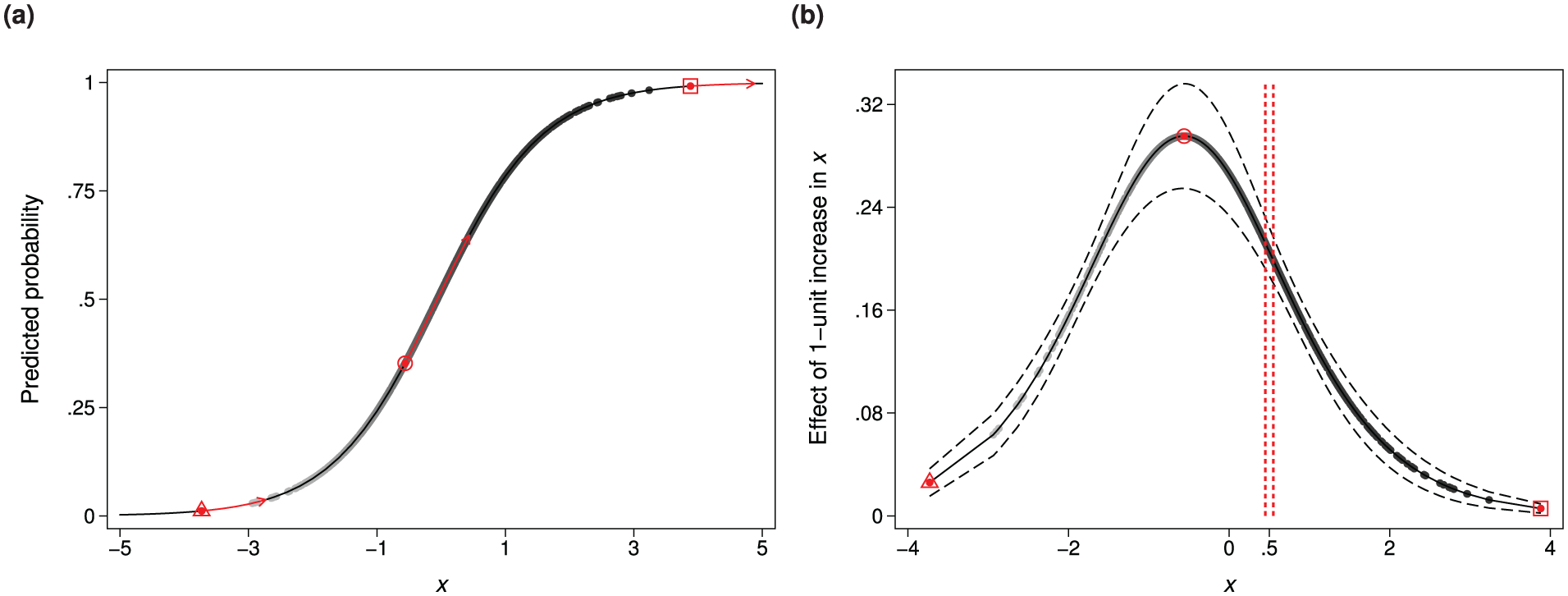
The effect of
Multivariate and alternative model specifications
Model b in Table 1 shows the regression results from an additive multivariate model (
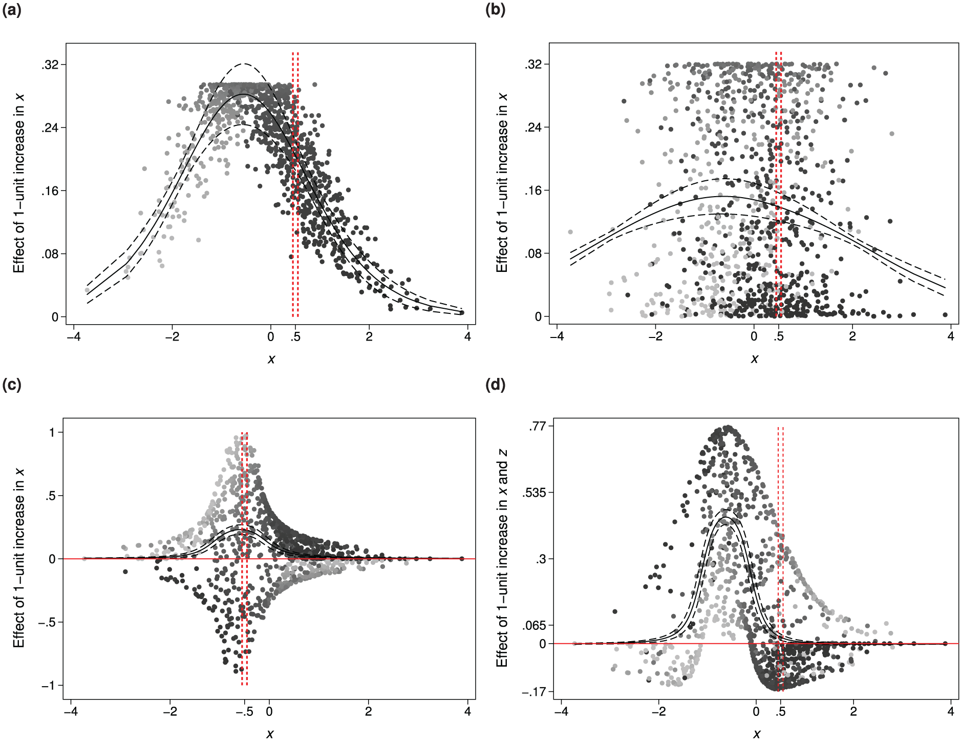
The effect of
Logistic regression results with simulated data.
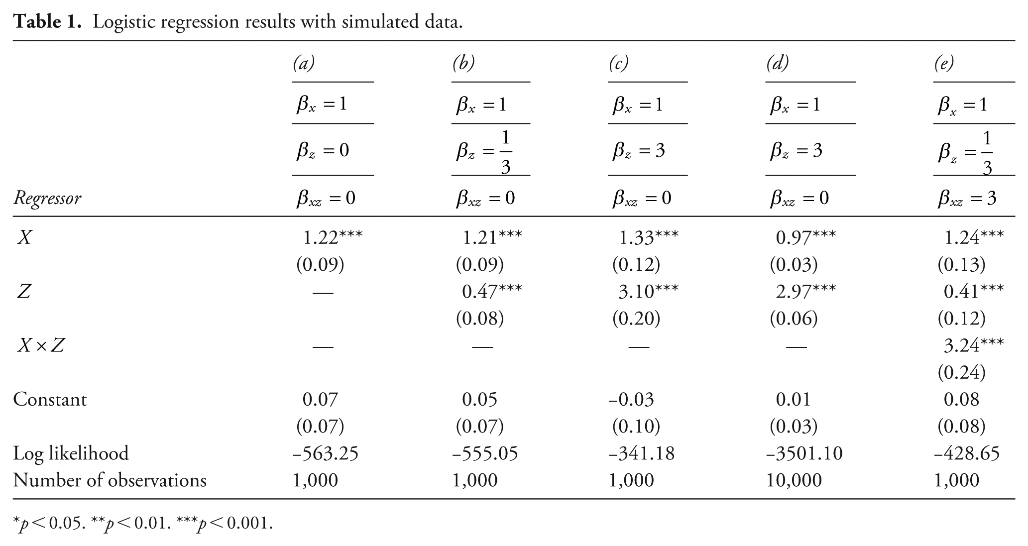
p < 0.05. **p < 0.01. ***p < 0.001.
Model 1a shows the regression results from a model where
The average effect deflation as
The effect of a 1-unit increase in
When
What explains the vertical variation in marginal effects at
So far, all our simulations have had the same sample size, i.e.
Lastly, we consider a scenario entailing interaction effects, for which
Figure 2c shows the conditional effect of a 1-unit increase in
Figure 2d shows the effect of a 1-unit increase in both
Potential criticisms
Researchers often acknowledge the horizontal variation in effects (over the range of
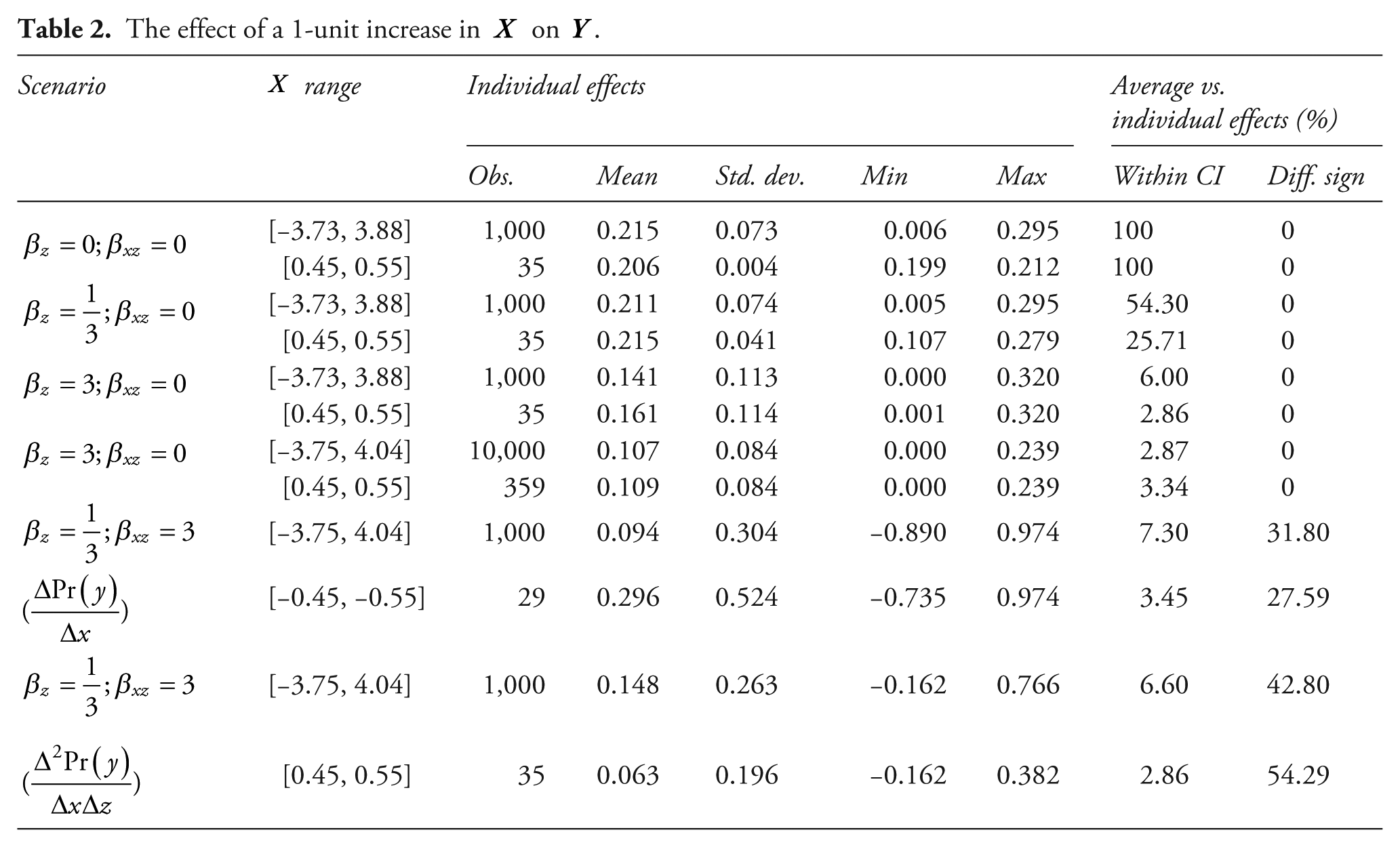
Others may point out that by using the average value as a fixed reference point, we neglect its variance. The argument would be that, while the point estimate of the mean does not match individual observations, the CI around it must contain a significant share of cases. Yet there is no theoretical reason to expect that it does. The CI captures uncertainty in the estimation of the average effect due to sampling uncertainty, not variation of cases around the mean. Other factors, such as sample size, also affect the CI width. The second to last column in Table 2 provides strong evidence for this. While all observations fall within the CI of the average effect when
One may also argue that by de-emphasizing the average effect we place too much weight on outliers. First, thinking of observations in terms of outliers is theoretically problematic when cases are of individual relevance. Going back to the civil war example, should we dismiss countries with high risk of conflict as noise? Second, there are analyses where ‘outliers’ are more representative for the cases at large than the mean. Using the data from the model where
Real data examples
Making inferences about individual cases based on the average response (under the assumption that the mean summarizes the population well), is not a theoretical problem but rather a practical issue with substantive implications. Using real data from three published studies, we showcase that reporting solely the average effect can lead to gross generalizations or incorrect inferences. The upcoming analyses are meant to exemplify some of the practical problems associated with the average effect, not to single out the respective studies.
Wealth and the risk of civil war
The first example reproduces Muchlinski et al.’s (2016) analysis of civil war onset, which we referenced in the introduction. The data consist of country-years between 1945 and 2000. The dependent variable, Civil war onset, is a dummy coded 1 when a civil war breaks out, and 0 otherwise. Following Muchlinski et al., we control for a host of potential determinants: ln(GDP/capita) records countries’ gross domestic product per capita, log-transformed; ln(Population) indicates the size of the population; ln(% Mountainous terrain) captures countries’ terrain ruggedness; Prior war is coded 1 if a country had experienced another war in the past; Non-contiguous territory is a dummy variable identifying countries that have non-adjacent territories; Oil exports/GDP captures countries’ reliance on oil as a proportion of the GDP; New state is a dummy identifying states that are less than two years old; Political instability is coded 1 if Polity records a change to 77 or 88 in the previous three years; Democracy is a regime dummy that equals 1 if the Polity score for a given country-year is a 6 or above; lastly, Ethnic fractionalization and Religious fractionalization are indexes that capture countries’ heterogeneity on the respective dimensions.
Table 3 reports the results from a logistic regression. Using the coefficient estimates and covariates’ observed values, we compute two of the most common substantive quantities of interest, that is, predicted probabilities and marginal effects (see Figure 3). Specifically, the solid line in Figure 3a graphs the average predicted probability and its 95% CI over the range of ln(GDP/capita). Departing from the standard approach, we also plot the individual probabilities for all cases in the data. These are indicated by solid circle marks. There are a couple of points worth noting. First, the spread of individual probabilities is substantively wider than what the average value and its CI imply. While the average predicted probability is 1.6% (1.3, 1.9), the individual probabilities range from 0.1% to 53.2%. Moreover, the 95% CI of the average probability includes only 26% of the cases. Put differently, 74% of the observations lie outside of the mean’s CI.
The determinants of civil war onset.
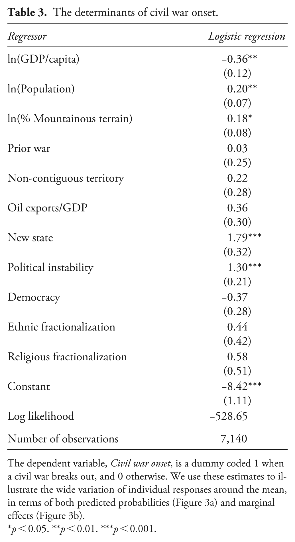
The dependent variable, Civil war onset, is a dummy coded 1 when a civil war breaks out, and 0 otherwise. We use these estimates to illustrate the wide variation of individual responses around the mean, in terms of both predicted probabilities (Figure 3a) and marginal effects (Figure 3b).
p < 0.05. **p < 0.01. ***p < 0.001.
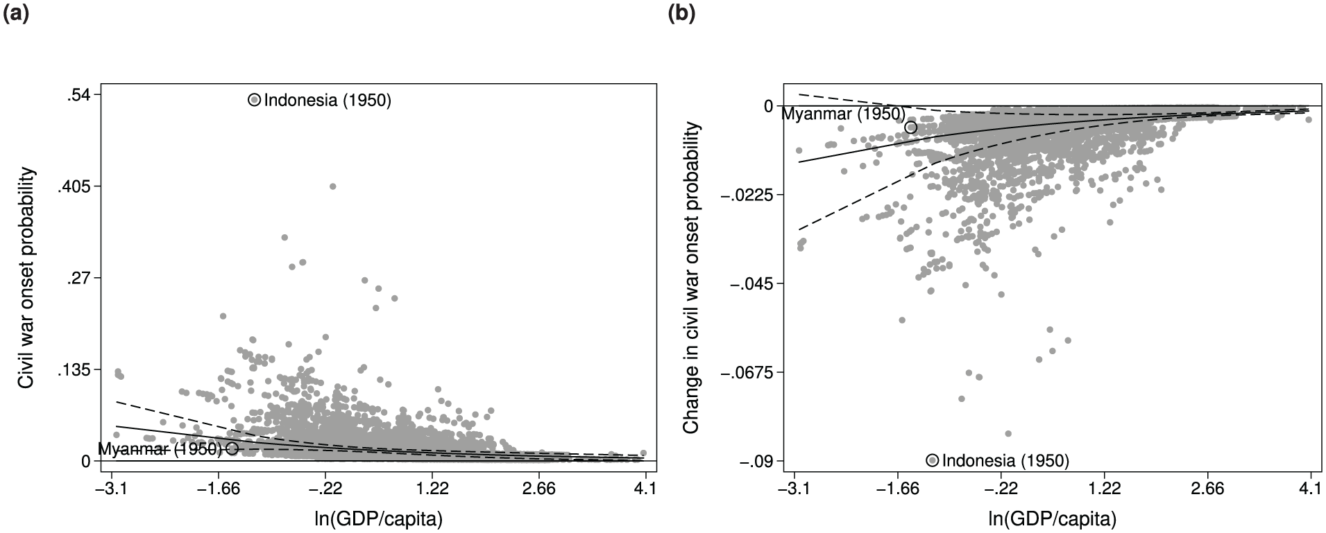
Conventional predicted probability and marginal effect plots.
For the marginal effect plot, Figure 3b, we compute the effect of a 1-unit increase in ln(GDP/capita), while the other variables are set at their observed values. As an indicator of state capacity, GDP is one of the best predictors of civil war onset (its coefficient is large and statistically significant), and one that is actionable (in contrast to ethnic and religious fractionalization, terrain ruggedness, etc.). The average marginal effect is −0.5 percentage points (−0.7, −0.2). While statistically significant, this is not a substantively meaningful effect. Arguably, a decrease in the probability of war onset from 1.6% to 1.1%, does not warrant acting in practice. Notably, a 1-unit increase on the logged scale corresponds to tripling GDP per capita on the untransformed scale: ln (GDP/capita) + 1 = ln (GDP/capita) + ln (e1) = ln (GDP/capita × 2.7). Thus, the meager effect is not an artifact of a small increase in wealth. In terms of the number of cases within the 95% CI of the average effect, less than half of the observations are included (43%).
Substantive considerations
For any given value of wealth, there can be quite a spread in the quantity of interest; this is the vertical variation we discussed in the technical section. For instance, Indonesia in 1950 has the highest risk of civil war onset, 53%, as well as the largest marginal effect, −9 percentage points. Indonesia’s high risk of civil war is not a deterministic outcome of its relative low level of wealth, but rather a consequence of its particular characteristics captured by the other covariates. Indeed, there are many cases that feature similar levels of wealth, for which the probability of war onset and the effect of wealth are near 0. For instance, in 1950, Myanmar was poorer than Indonesia. But its risk of civil war is about 0.5%, and the counterfactual 1-unit increase in ln(GDP/capita) decreases the risk by only 1.8 percentage points. These two cases are highlighted in Figure 3.
Given the wide variation in individual effects, the average marginal effect does not represent a reasonable value for the change in the risk of civil war for any given country – not even on average. Specifically, it is not the case that if we were to repeatedly increase GDP in a long sequence of counterfactual experiments, the mean prediction for individual cases would be close to −0.5 (the population average). In fact, the mean prediction for our cases are the scattered values outlined in the marginal effect plot (e.g. −9 for 1950 Indonesia). An insidious problem stemming from a deflated mean is that it may lead policy makers to overlook an effective strategy simply because it is not optimal in different country contexts. A medical analogy would be the case of a patient forgoing a personalized treatment based on their genetic profile, because the effectiveness of that treatment in the population at large is relatively low.
The correct interpretation of the average effect may prevent unwarranted extrapolations, but does not solve the problem of the lack of practical relevance. Specifically, the worldwide propensity of civil war, which indiscriminately pools stable and less stable countries, is of little real-world relevance. For concreteness, the mean value represents the average change in the global risk of civil war, if all countries were to increase their wealth by the same amount. While convenient for practical calculations, such a concerted effort is not a realistic counterfactual. Moreover, it is not the case that one country can offset another country’s (in)action. Specifically, the average risk would be different if two countries, A and B, increase their wealth by the same amount n, compared to when A’s wealth increases by 2×n while B’s wealth stays the same. Ultimately, from the average effect we cannot infer a country’s risk of civil war conditional solely on its economic performance. Yet this is the relevant information for practical applications, since governments do not have control over economic policies in other countries.
In sum, the average can obscure a large variation in the values that created that score. On the one hand, one cannot really criticize the mean for not showing the full spread of the underlying data points. On the other hand, we need to acknowledge that the mean does not always summarize the population well. This can be of significant relevance for practical case applications, especially when cases carry special meaning.
Wealth, weather shocks, and political violence
In the previous section, we showed that the mean value can lead to gross generalizations (i.e. the average response misrepresents individual effects by several orders of magnitude). More problematically, the average value can also lead to incorrect inferences (i.e. individual effects having the opposite sign than that of the average effect, or subgroups of cases exhibiting opposite trends). We illustrate this problem using a model of peace, repression, and civil war from Bagozzi et al. (2015), which in turn is a replication of Besley and Persson (2009).
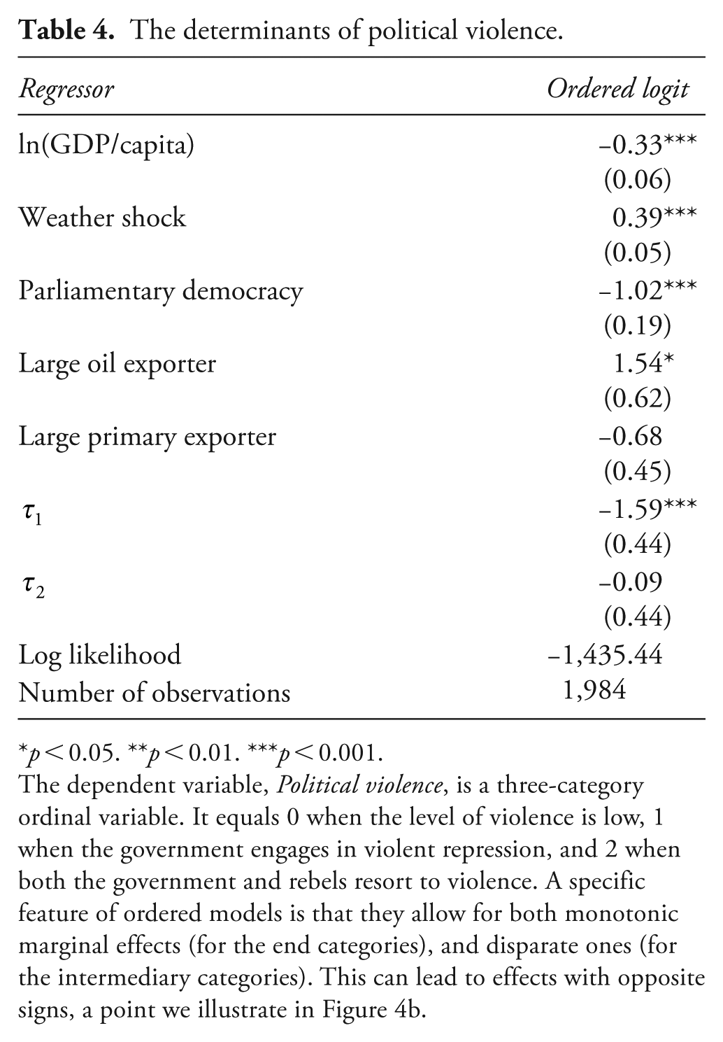
The dependent variable, Political violence, is a three-category ordinal variable. Specifically, it equals 0 when the level of violence is low, 1 when the government engages in violent repression, and 2 when both the government and rebels resort to violence (i.e. civil war). The explanatory variables are the same as in Bagozzi et al. (2015): ln(GDP/capita) is the standard indicator for economic development; Weather shock is a count of the number of floods and heat waves that countries experience each year; Parliamentary democracy captures the institutional setup; Large primary exporter equals 1 if, in a given year, more than 10% of a country’s GDP is generated by product exports, and 0 otherwise; lastly, Large oil exporter equals 1 if more than 10% of a country’s GDP is generated by oil exports.
Table 4 reports the results from an ordered logistic analysis. A key finding in Besley and Persson (2009) is that wealth decreases the probability of violence. This finding is illustrated by the average effect plots in Figure 4, which show the effect of a 1-unit increase in ln(GDP/capita) while holding the other covariates at their observed values. More specifically, the solid lines outline the mean effect and the dashed lines are the 95% CI. Specifically, Figure 4a indicates that, on average, wealth has a positive effect on the probability of peace. Conversely, increasing GDP decreases the probability of both repression, Figure 4b, and civil war, Figure 4c. In all three scenarios, the magnitude of the effect decreases as wealth increases. 10
The determinants of political violence.
p < 0.05. **p < 0.01. ***p < 0.001.
The dependent variable, Political violence, is a three-category ordinal variable. It equals 0 when the level of violence is low, 1 when the government engages in violent repression, and 2 when both the government and rebels resort to violence. A specific feature of ordered models is that they allow for both monotonic marginal effects (for the end categories), and disparate ones (for the intermediary categories). This can lead to effects with opposite signs, a point we illustrate in Figure 4b.
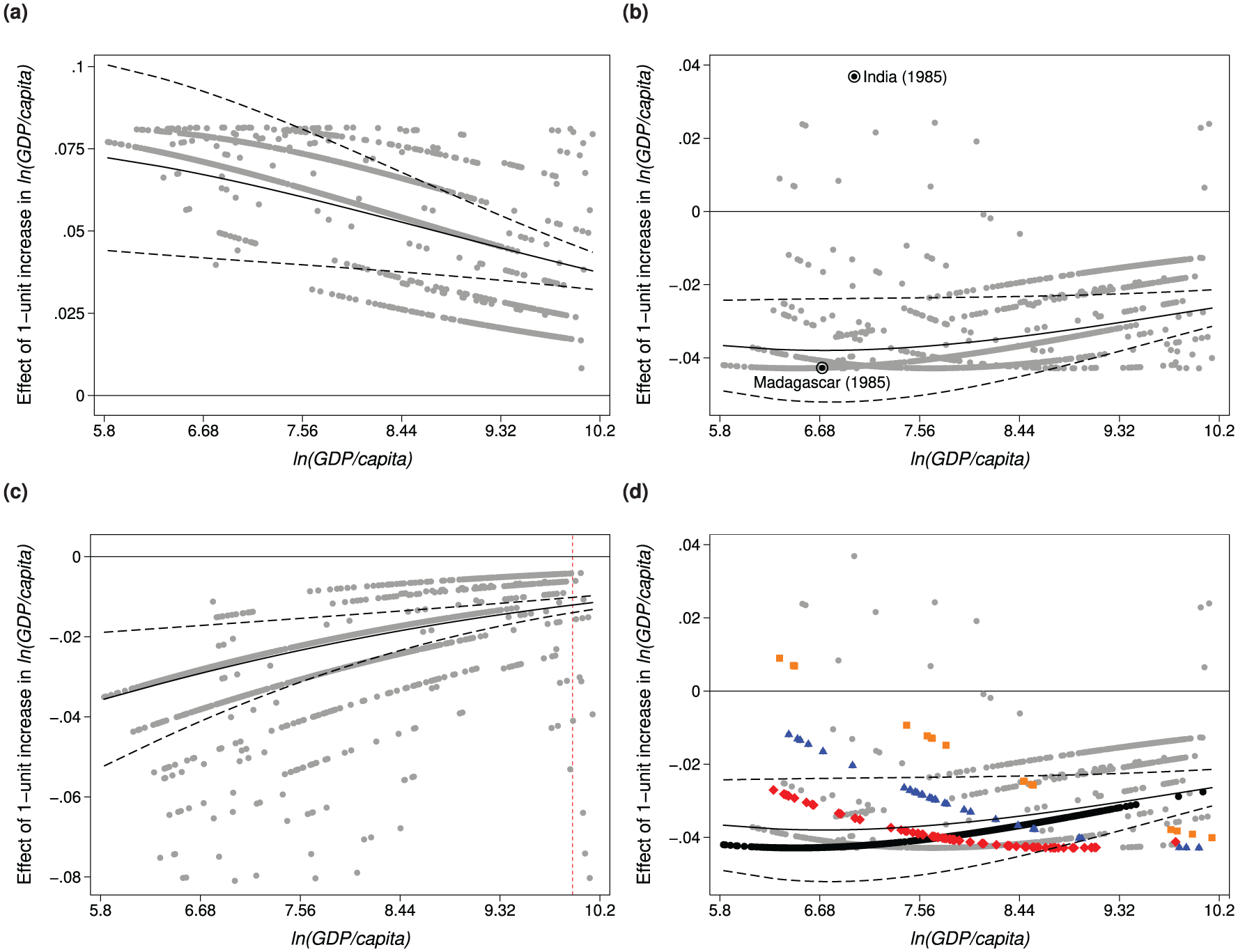
The effect of ln(GDP/capita) on the probability of political violence.
Besides the average effect, we also plot the effect for all cases in the data (the gray dots). The wide variation in individual effects provides a more nuanced picture of the effect of wealth on political violence. As an illustration, let us consider the effect of wealth on the probability of civil war for ln(GDP/capita) values higher than 9.96. This is the area to the right of the vertical dotted line in Figure 4c. We focus on this wealth interval because the CI is at its narrowest, which would suggest that the uncertainty around the average value is low. The average effect for the 13 cases within this interval is −3.3 (−4.0, −2.5). But the observations are spread out (the range is [−8, −0.4] percentage points), and only one is contained by the average effect’s 95% CI. What is more, the subsample’s standard deviation is twice the size of the one for the entire sample, 2.58 vs. 1.25. Importantly, we would not be aware of the magnitude of the vertical variation in individual effects, if we had plotted only the average effect.
The discrepancy between the average and individual effects is most striking in the repression scenario, Figure 4b. While the average effect is always negative, there are cases with positive marginal effects at both low and high values of wealth. For a concrete example, consider India and Madagascar which had similar GDP/capita levels in 1985. Because of country specific attributes, increasing wealth decreases the risk of government repression in Madagascar by 4.3 percentage points. By contrast, the same economic boost increases the risk in India by 3.7 points. These diametrically different effects are both statistically significant (p < 0.01). More generally, for the level of wealth India had in 1985, the average effect is −3.8 percentage points. Given the opposite direction, it is ill-advised to make policy recommendation for India based on the average effect. 11
Opposite effects aside, there are subgroups of cases with a different effect pattern than the average trend. Figure 4d highlights four such subgroups. The cases in the respective subgroups differ solely in their experience with natural disasters (i.e. they have identical values on all other attributes). Recall that Weather shock is a count of the number of floods and heat waves that countries experience in a given year. As a reference point, the black dots indicate the cases that were spared by extreme weather events. Since these observations represent about 40% of the data, the average effect line closely follows their trajectory. For this subgroup, increasing GDP/capita reduces the probability of repression, and the magnitude of the effect decreases as wealth increases.
The average pattern, however, is not representative for the subgroup of countries that have experienced natural disasters. Specifically, in red with diamond marks are the countries that experienced 2 weather shocks; in blue with triangle marks are the countries with a score of 3; and, in orange with square marks are the countries with a score of 4. In contrast to the diminishing magnitude of the average effect, the size of the effect increases with the levels of ln(GDP/capita) in countries affected by natural disasters. Moreover, the rate of change (i.e. the slope of the effect line) becomes steeper with the frequency of weather shocks. By looking solely at the average effect, we would be aware of neither opposite effects nor opposite trends in our data.
Democratic survival in post-civil war settings
In this section, we replicate an analysis from Graham et al. (2017) on the impact of inclusive institutions on democratic survival, conditional on states’ experience with civil conflict. The dependent variable, Democracy, equals 1 if the executive and legislature are fairly elected, and a majority of adults have the right to vote. It is coded 0 otherwise. Besides a number of control variables (Ethno-linguistic fractionalization, Regional polity, GDP/capita, GDP growth, Fuel dependence, Population, Past democratic breakdowns, and Democracy age), the analysis includes three two-way interactions between Post-civil war and Inclusive, Dispersive, and Constraining power-sharing. The estimation model is a probit, and the regression results are presented in Table 4, Model 1 (Graham et al., 2017: 699). According to the authors, the findings show that constraining powersharing helps democratic survival generally, inclusive powersharing only in post-civil war settings, whereas dispersive powersharing may be detrimental for democracy.
Figure 5a shows the average effect of post-conflict status on the probability of democratic survival across the range of inclusive powersharing (from the 5th to the 95th percentile). More specifically, this figure shows the difference in the predicted probability of democratic survival for countries with and without a recently ended civil war, which the authors report in the top plot of Figure 3 (Graham et al., 2017: 700). 12 The difference in probability allows us to directly assess at what levels of inclusiveness the conditional effect is statistically significant. By constrast, when examining the individual probabilities side by side, we cannot tell whether the two are distinct when their CIs overlap (Gelman and Stern, 2006; Radean, 2023b). The average conditional effect is small and statistically insignificant at low levels of inclusive powersharing, but increases quickly with inclusiveness.
Figure 5b shows the same effect with the individual effects superimposed. As a reference point, we identify the Pakistan case that the authors reference. The dotted vertical line delineates the below and above average inclusiveness levels. 13 There are a couple of things worth noting. First, with the highest value of 6 percentage points, the average effect absconds substantively large effects in the population (min = −21, max = 53). In fact, the putative null effect at low levels of inclusiveness (with a nominal level of less than 1 percentage point) is an artifact of large positive and negative effects (some as high as |21| percentage points) canceling each other out. Second, 30% of individual effects have the opposite sign than that of the average. We highlight four such observations, representing conflict-free and post-conflict states (names in italics) at below and above average level of inclusive power-sharing. Given the high share of observations that buck the trend, policy recommendations based on the average effect are tenuous.
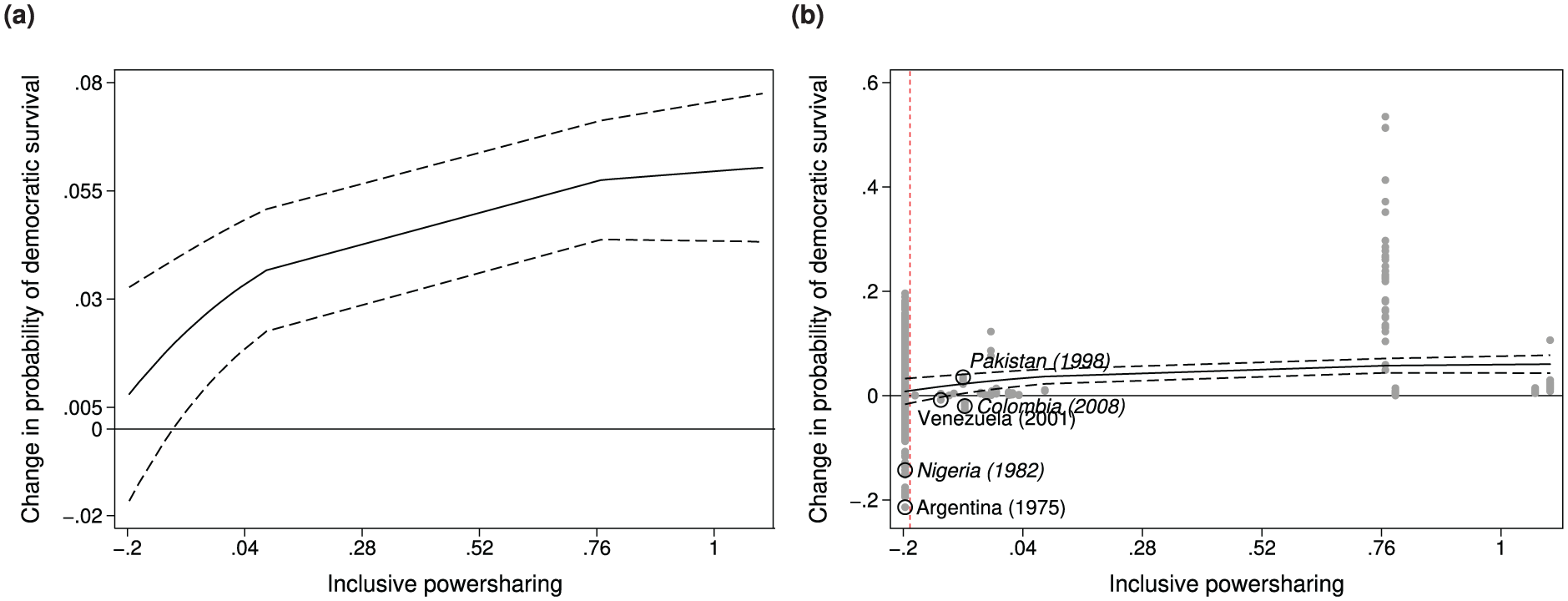
The conditional effect of past civil war experience on democratic survival.
On the basis of the average response in the population, the authors make policy recommendations for both domestic institution-builders and international organizations. More specifically, they name half a dozen countries to which the study’s findings should apply, but no individual effects are reported. This includes out-of-sample cases, for which it is not even possible to estimate individual responses since we do not have the necessary information (i.e. the value of model covariates). As an example, the authors argue that, considering the efforts to ‘stabilize democratic transition in Burma’, international actors should rethink their push for inclusive powersharing and decentralized institutions (Graham et al., 2017: 702). Yet Burma is a dictatorship for the entire timeframe of the study (1975 to 2010). Given the available information, we cannot use the model estimates to assess democratic Burma’s odds of survival. While some country attributes are not affected by the democratization process (e.g. ethno-linguistic fractionalization), others are bound to change. At the very least, the constraining dimension of powersharing (i.e. the extent institutions constrain political leaders) would change as Burma transitions from dictatorship to democracy. Of course, one may impute not-yet-observed values using valuations of country experts, or by employing some other technique. But this would then be a forecasting exercise, which is not the case here.
Conclusion
To convey the substantive importance of their research findings, political scientists commonly compute the average effect in the population. There are instances, however, when a single value is too generic to be meaningful when applied to specific cases. In particular, the mean can obscure a large variation in individual effects, and may lead to gross generalizations or incorrect inferences. Crucially, we cannot tell a priori whether individual responses are close to the mean or dispersed, and often used heuristics can be misleading (e.g. the CI width of the average effect).
To improve empirical practice, we make two recommendations to substantive researchers:
The problem we highlight in this article is not a small sample issue, and collecting more data would not necessarily help. Similarly, correctly interpreting the average effect may prevent unwarranted extrapolations, but does not solve the problem of the lack of practical relevance. Case in point: what practical recommendations can we draw from the finding that doubling the GDP of all countries in the world reduces the global risk of civil war by less than half of a percentage point?
Our recommendations are particularly relevant for analyses where cases carry special meaning. In such instances, discussions about practical or substantive significance ought to take place at the individual level. This type of analysis is common in political science. In international relations, the canonical data comprise countries extant at a given time. In American state politics, the unit of analysis are the 50 US states. This is also the case in comparative politics research that focuses on party politics or legislative behavior.
A good rule of thumb when deciding the appropriate level for model evaluation, is to think about the level at which policy recommendations make sense (e.g. individual, subgroup, population). If the study is about the effect of an initiative to increase voter turnout, we cannot and should not focus on the idiosyncratic responses of individual voters. In this case, it is the average response that is of immediate interest. Conversely, if we assess the effect of wealth on the likelihood of civil war onset, we are interested in individual responses – particularly those of countries on the brink of civil war. In this case, the average response is not particularly informative.
Lastly, we address a couple of possible concerns. One potential criticism is that researchers are well aware of the limitations of the average effect. If that were the case, making policy recommendations based on the average response would be the exception; yet it is the norm. Another concern is that case-level estimates are less reliable, since they are more sensitive to model specifications than the average value. That is a valid concern. However, using a robust but disparate average value, possibly with an opposite sign, is not the solution. The better approach is to conduct sensitivity analyses checking whether the case effect of interest is robust, and we urge researchers to do so. The appropriate robustness test for practical relevance is the effect strength stability, not the standard significance-robustness test. This means testing whether the estimated effect size is substantively different across various model permutations, rather than whether the estimated effect keeps its sign and significance status (Neumayer and Plümper, 2017).
Some may also point out that not all researchers are interested in discussing specific cases. But analysts who present evaluations of substantive effects or policy recommendations, implicitly demonstrate an interest in making a connection between research and practical applications. Our recommendations help assess the distance between theory and practice, and make applications to specific cases more realistic. While rooted in technical considerations, our concerns are substantive in nature. In analyses where the mean is not a representative central value, its practical significance is brought into question. Due to a lack of substantive relevance, researchers have been advised against making big claims about small and practically inconsequential effects – even if they are statistically significant (Esarey and Danneman, 2015; Gross, 2015; Rainey, 2014). Pushing the argument further, we argue that the substantive significance concern extends to situations where researchers focus on non-actionable average effects.
Footnotes
Acknowledgements
We thank Dominik Duell, Justin Esarey, Daniel W Hill Jr, Sara MT Polo, and Jonathan Slapin for their helpful comments and suggestions.
Funding
The authors received no financial support for the research, authorship, and/or publication of this article.