
Abstract
Have great wars become less violent over time, and is there something we might identify as the long peace? We investigate statistical versions of such questions, by examining the number of battle-deaths in the Correlates of War dataset, with 95 interstate wars from 1816 to 2007. Previous research has found this series of wars to be stationary, with no apparent change over time. We develop a framework to find and assess a change-point in this battle-deaths series. Our change-point methodology takes into consideration the power law distribution of the data, models the full battle-deaths distribution, as opposed to focusing merely on the extreme tail, and evaluates the uncertainty in the estimation. Using this framework, we find evidence that the series has not been as stationary as past research has indicated. Our statistical sightings of better angels indicate that 1950 represents the most likely change-point in the battle-deaths series – the point in time where the battle-deaths distribution might have changed for the better.
Introduction
Is the world becoming more peaceful? The question is both deceptively simple and quite controversial. Authors such as Gat (2006), Goldstein (2011) and Pinker (2011) have argued that the world is becoming steadily more peaceful, and a multidimensional quilt of research has contributed pieces of layers with similar stories and conclusions. 1 Parts of these arguments concern wars and armed conflicts, and there, the concept of ‘the long peace’ (Gaddis, 1989) has gained the weight of repeated respectful use, to signal the relatively few large interstate wars in the period after World War II (WWII).
While the empirical pattern constituting the long peace is not in itself disputed, some recent investigations have questioned whether the pattern can be said to constitute a statistically established trend (see e.g. Cirillo & Taleb, 2016; Clauset, 2017, 2018; Braumoeller, 2019). Could this long period of relative peace simply be a random occurrence in an otherwise homogeneous war-generating process, or does it represent a significant change, a trend towards peace? Cirillo & Taleb (2016), Clauset (2017, 2018) and Braumoeller (2019) answer the last question negatively: they find that the long peace is not a sufficiently unusual pattern when considering the variability inherent in long-term datasets of historical wars. The question investigated by these authors is essentially statistical in nature, and we follow in the same vein. We approach a similar question, with similar data, but with somewhat different statistical tools.
We see our contribution as two-fold. First, we introduce a set of statistical methods to the peace research community, some of them new. We have attempted to make the presentation of the methods accessible to most peace researchers. Technical details, of separate interest also to specialists in statistics, are placed in the Online appendix. Second, we present new results and conclusions that partly challenge previous works and may generate hypotheses that can form the basis of future investigations. We find evidence that a sequence of war sizes from the last two centuries is not entirely homogeneous. In this sequence, the point of maximal change is found in 1950, corresponding to the Korean war. The upper quartile of the battle-deaths distribution decreases substantially, from 63,545 before the Korean war to 14,943 after. Note that there is considerable uncertainty around these estimates and that the conclusion is open to interpretation. Our change-point analysis gives a very wide 95% confidence interval for the point of change, but it also places considerable confidence on only a small handful of wars, including the Korean war, which is the maximum likelihood estimate. The uncertainty is discussed in detail below. We differ from parts of the literature by not focusing exclusively on WWII as the potential point of change, but by applying change-point methodology to investigate distributional changes in a time series of wars. We also investigate the role of covariates, in particular democracy.
In the next section we draw on the existing literature to sharpen the question we will be considering. We also present the data we will use and discuss the overall analysis framework. Then in the following section, we present the relevant statistical methods in more detail. Next, we present our main results: first we perform a homogeneity test, and as this indicates non-homogeneity we go forward with change-point methodology, and crucially also present the degree of change. Then we investigate the effect of democracy. In the final section, we discuss our findings: we examine the robustness of our approach to various choices and its relationship with previous works, and also consider potential theoretical mechanisms.
War sizes and onset times in the CoW data
Modelling wars
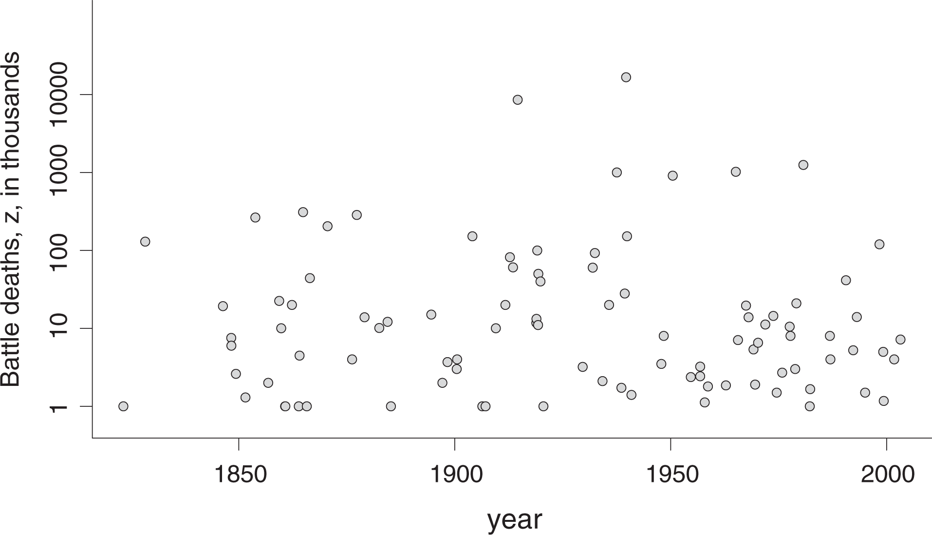
Efforts to uncover trends in armed conflict have a long history and date back at least to the seminal contributions of Lewis Fry Richardson (1948, 1960). Richardson assembled datasets of historical wars and sought to uncover long-term patterns by statistical modelling of various quantities, for example the time between wars and also the number of fatalities in each war. We will consider the Correlates of War (CoW) interstate conflict dataset (Sarkees & Wayman, 2010), see Figure 1, which we discuss in a bit more detail below. For now, consider a general war dataset consisting of

for a number n of historical wars, where xi
is the onset time of war i and zi
the number of fatalities; henceforth we will call zi
the size of war i. Richardson’s analyses of historical wars led him to two important statistical insights: the between-war times the war sizes zi
can be modelled as i.i.d. with a power law distribution.
Both the time between wars and the size of each war are relevant for investigating whether the world has become more peaceful. A peaceful world could be characterized by fewer wars (i.e. longer time between wars), smaller wars, or both. Note a potential caveat concerning the assumed connection between a decline in war sizes and arguments about whether the world is becoming more peaceful. Fazal (2014) argues that the risk of dying in war has declined because of the revolution in military medicine: war may see just as many casualties as before but fewer deaths, since modern medicine is able to save more lives. We will not explore this hypothesis in our article.
Trends in the number of interstate wars have been studied by, for example, Harrison & Wolf (2012), Gleditsch & Pickering (2014), Cirillo & Taleb (2016), Braumoeller (2019) and Clauset (2018). Harrison & Wolf (2012) claim that interstate wars have become more frequent over time, while Gleditsch & Pickering (2014) criticize their approach and claim that wars are in fact becoming less frequent. Clauset (2018) finds that the time between wars in the CoW data is adequately modelled by a simple exponential distribution, a finding that supports insight (i) of Richardson above. Clauset (2018) takes this finding as an indication of a lack of trend in the war timings data. In the Online appendix we provide a short investigation of the between-war waiting times di in the CoW dataset and find that the observed waiting times are more consistent with an exponential-gamma mixture model than with a simple exponential model. This indicates that the waiting times in the CoW dataset are more variable than expected under an exponential model. For the rest of the article we will leave the waiting times aside and focus on the war sizes.
Richardson’s second insight has possibly received even more attention than the first one. Power laws are a particular class of probability distributions, with

and a positive parameter θ. This means that the probability of observing an event, in our case a war, of size larger than z is inversely proportional to z raised to θ. If θ is large this probability quickly decreases with z, but if θ is smaller
Richardson’s insights concerning power laws are discussed by Pinker (2011) in his international best-seller The Better Angels of Our Nature. There, he argues that violence in a wide sense, including crime, torture, animal cruelty and war, has declined. Power laws also form the basis of empirical investigations that challenge Pinker’s conclusions about the decline of war and the long peace. In Cederman, Warren & Sornette (2011), a sequence of 118 war sizes from 1495 till 1997 is modelled with power law distributions. The authors find a shift in the power law parameter in 1789, indicating larger wars after that year compared to the period before. Cirillo & Taleb (2016) build their own database of war deaths from year 1 to the present. They use statistical models with power law tails and find that their dataset is well enough described by a single, stationary model. Clauset (2017, 2018) examines the CoW data discussed below, models the size of interstate wars with power laws, and finds that he cannot reject the null hypothesis of no change. Indeed, he argues that the current trend would have to persist for 150 years until we could statistically claim that the world had become more peaceful.
Now we have decided on a quantity of interest, war sizes, and have found a class of appropriate statistical distributions to model this quantity. Still, there is a major question to resolve: should we normalize the war sizes by population size or should we consider the absolute number of fatalities instead? Here, normalization refers to dividing the number of fatalities by the population size, typically the world population. Pinker (2011) forms most of his arguments around relative quantities, such as deaths per 100,000. Clauset (2017, 2018) discusses the choice of normalization in some length, and decides to analyse the absolute numbers. The choice of normalization in fact translates into different questions: are we interested in making claims about the absolute sizes of wars? Or the risk of dying in wars? And in the latter case, with respect to which segment of the population should this risk be defined? All these questions are valid and interesting, but naturally the answers to one of them will not be directly relevant for the others. We have chosen to consider the absolute numbers. For the proponents of the long peace theory this is a conservative choice since normalizing by world population inflates the size of ancient wars compared to more recent wars.
Further, there is a choice between different datasets. Naturally, we would prefer a dataset stretching as far as possible back in time, with measurements of high quality and constructed with careful and precise definitions. The previously mentioned study by Cederman, Warren & Sornette (2011) combines data from Levy (1983), the CoW project (Singer & Small, 1994) and the PRIO/UCDP Armed Conflict Database (ACD) (Gleditsch et al., 2002). The dataset has a long time span, but is unfortunately limited to wars involving ‘major powers’. The quality of the reported battle-deaths number can also be an issue. Even for recent wars involving developed countries the estimates of the number of battle-deaths can be contested. The Falklands war, for instance, is included in the CoW interstate wars dataset with 1,001 battle-deaths, even though the actual number is most likely closer to 900 (Reiter, Stam & Horowitz, 2016).
We have used the Correlates of War (CoW) interstate conflict dataset (Sarkees & Wayman, 2010). This dataset contains onset dates xi and the number of battle-deaths zi for all interstate wars with more than 1,000 battle-deaths in the period 1816 to 2007, comprising a total of 95 wars. The dates xi range from 1823.27 (the Franco-Spanish war) to 2003.22 (invasion of Iraq). Figure 1 displays these data, with zi on the log10-scale. The choice of the CoW dataset is motivated by its widespread use (Clauset, 2017, 2018; Fagan et al., 2018; Spagat & van Weezel, 2018), which enables comparisons with other approaches. Also, the CoW dataset is considered to be of good quality, despite the issue mentioned above.
Finally, there are several different statistical frameworks for assessing whether a certain sequence of observations, war sizes in our case, supports a trend, or not. The possible options include regression models with respect to time, homogeneity tests and change-point analyses. We have not investigated regression models as these would impose too much of a constraint on the type of change present (also a quick look at Figure 1 clearly indicates that there is no simple linear time trend).
Homogeneity tests are a general class of methods which aim at testing a null hypothesis of stationarity, that is, to test whether the observed sequence is consistent with a single, stationary statistical model or whether there is sufficient deviation from the model as to indicate that there has been a change. Most of the results in Clauset (2017, 2018) are based on tests of homogeneity, where Clauset does not find sufficient evidence to reject the null hypothesis of no change. Tests of homogeneity seem attractive because they can potentially discover many types of deviations from the stationary model. However, for partly the same reason, they can often have low power in discovering actual changes. There are many homogeneity tests to choose between, which differ in, for example, the assumptions made, the choice of test statistic and the choice of alternative hypothesis; see Hjort & Koning (2002) and Cunen, Hermansen & Hjort (2018) for partial reviews and methods. We present a general homogeneity test in the methods section.
If the null hypothesis of homogeneity is rejected, there may be reasons to believe that the data are inconsistent with a completely stationary model. The rejection of the hypothesis does not necessarily give any indication on where the change took place, nor what type of changes the data support. Change-point analysis is a framework for investigating a certain type of ‘trend’: an abrupt change in the distribution of the data, with particular emphasis on where the change took place. There is a long tradition in social and political science for studying shifts in history, and for examining conditions for the potential for shifts (see Tilly, 1995; Marx, 1871; Spengler, 1918; and e.g. Beck, 1983; Mitchell, Gates & Hegre, 1999; Western & Kleykamp, 2004; Spirling, 2007; Blackwell, 2018). Change-point methods have been applied to sequences of war sizes in Cederman, Warren & Sornette (2011), and very recently in Fagan et al. (2018) and Braumoeller (2019).
Methods
In the first subsection, we construct a non-parametric homogeneity test. Since this test indicates non-homogeneity (see the results section), we proceed with our change-point framework. First, we present parametric models for the war sizes, before presenting our change-point method. In the last subsection, we explain the inclusion of covariates.
Testing constancy over time
Suppose a sequence of observations
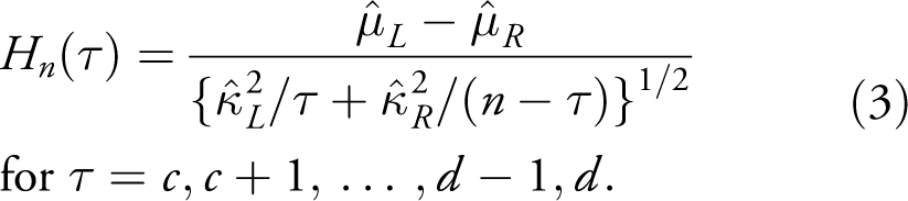
Here
Importantly, the Hn plot may be utilized for the one-sided case where a change is assumed to have a given direction, on a priori grounds, thus yielding bigger detection power than with a two-sided version. Also, the method works for non-parametrically defined μ. In order to find the p-value for the test, one needs to work out the distribution of the Hn process. We present these derivations in the Online appendix. There we also investigate a different homogeneity test based on a weighted Kolmogorov-Smirnov statistic.
Models with power law tails
In order to use the change-point method from Cunen, Hermansen & Hjort (2018) we need a parametric model for the war sizes, zi
. As discussed above, we want to use a model with power law behaviour. One general option is to use the power law distribution directly, see Equation (2). For most datasets, the power law distribution will not fit well for the entire dataset, but only for observations larger than a certain threshold, that is,
Another option is to model the entire dataset, which in our case only has wars of sizes 1,001 and more (see Online appendix Section D), with a distribution that fulfils the power law requirement in the tails. Generally speaking, the distribution function
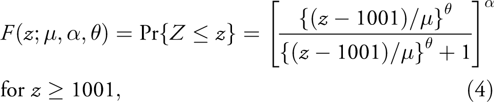
with parameters
There are other distributions with power law tails, and the choice between these models should ideally not influence the reported results to a great extent, as long as the chosen model has a reasonably good fit to the data. In the Online appendix, we examine goodness of fit, some model selection with the focused information criterion, and also report results using other parametric models.
Change-point methods
When faced with a sequence of observations, change-point methodology is used to search for where the point of maximal distributional change occurs. More formally, we have observations
There are many ways in which to search for a change-point in a sequence of data; see Frigessi & Hjort (2002) for a broad introduction to a special journal issue on discontinuities. Here we employ change-point machinery developed in Cunen, Hermansen & Hjort (2018), both for spotting a potential change-point and, crucially, for assessing its uncertainty. To assess uncertainty and present our result, we use confidence curves (see Schweder & Hjort, 2016). The confidence curves can be understood as graphical generalizations of confidence intervals. They present the uncertainty at all levels of confidence, instead of just a single confidence interval at some arbitrary level of confidence (typically 95%). See the results section for more on the interpretation of confidence curves.
In the Online appendix we provide a short technical overview of the change-point method we have used. The version of the method used here only allows for a single change-point in the sequence of data. Importantly, the method involves maximum likelihood estimators of the model parameters,
The change-point method of Cunen, Hermansen & Hjort (2018) also allows us to construct confidence curves for the degree of change associated with the change-point. The degree of change is a one-dimensional parameter, called ρ, defined as a function of the model parameters on both sides of τ, and meant to capture the size and direction of the change. Usually it will be in the form of a ratio or a difference; here we will study the ratio between quantiles of war sizes on each side of τ. Confidence curves for the degree of change,
In our analysis, we will use the change-point method briefly discussed here along with the inverse Burr model described in the previous section. In addition to the choice of distribution, the modeller also needs to decide on which parameters of the distribution should be allowed to be (potentially) influenced by the change-point. For the model in Equation (4), we allow θ and μ to change, but assume the same α across the change-point. We then end up with a total of six parameters to estimate: the change-point τ, along with
Covariates
The change-point method above is sufficiently general to support the inclusion of covariates influencing the model parameters, for example democracy scores, as we will see. For simplicity of presentation, we will present the inclusion of a single covariate to the inverse Burr model described above; in the Online appendix we give a more general treatment.
Assume that we have covariate information wi
for each war. In this illustration, the covariate is the mean democracy score of the countries involved in each war, measured the year before the war started. To measure democracy, we utilize the Polity index from the Polity IV dataset (Marshall & Jaggers, 2003). The Polity index scores regimes on a
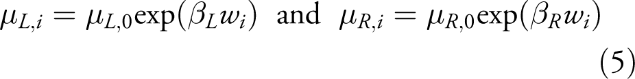
for i = 1,…,90.
Note that some of the wars have missing democracy scores. We remove these observations and end up with 90 wars for this analysis. The full model has now become moderately complex, with parameters
When introducing covariates in this change-point model, there are some issues to consider. First, one can either assume that the covariate effect has changed across the change-point, or that it has remained constant (so
Results
Testing constancy
For the sequence of log-battle-deaths The relative change Hn
plot of Equation (3)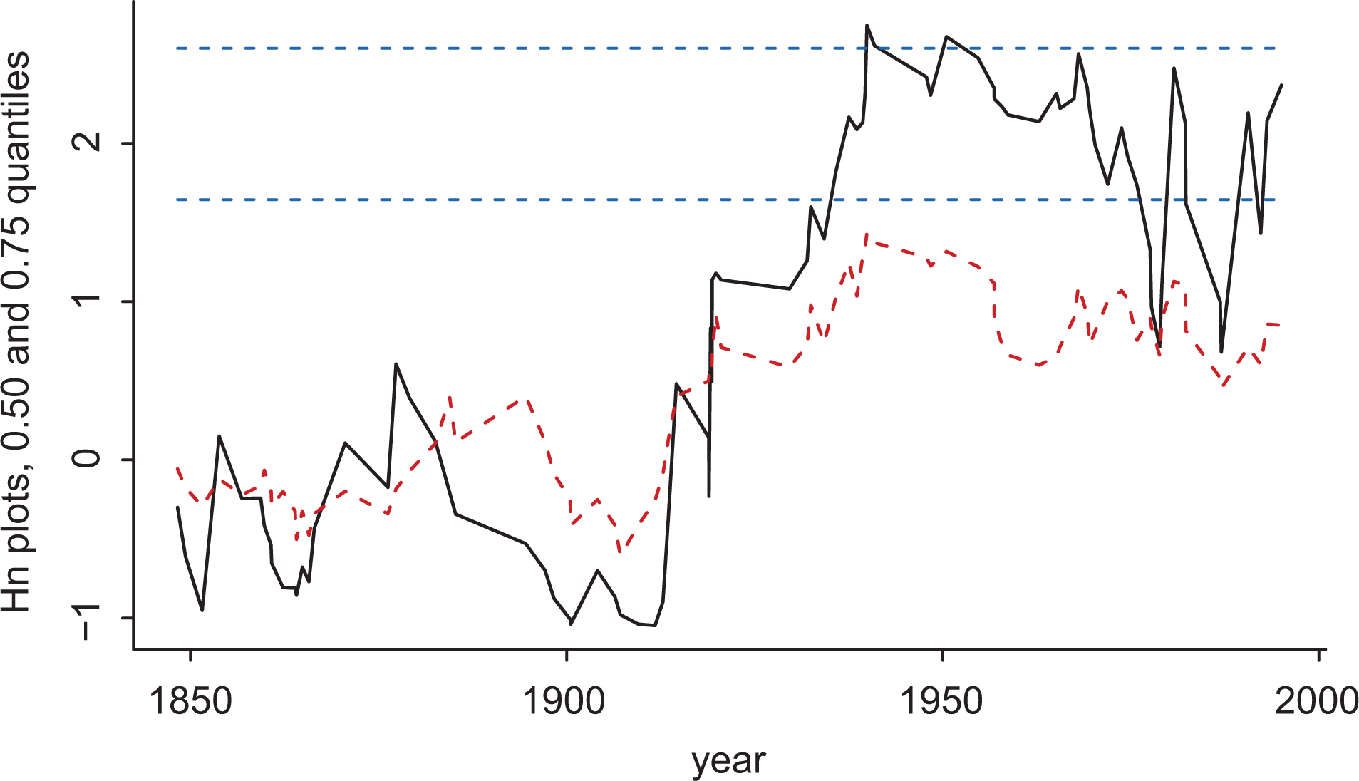
The p-values, for monitoring the no-change hypothesis with respect to quantiles, become even smaller for higher quantiles than 0.75. Thus the battle-death distribution has not remained constant over time. More specifically, plots such as those in Figure 2 reveal that there are clearer changes in the upper parts of the distribution than in the lower parts.
Change-point results
Our change-point method provides the maximum likelihood estimate for the change-point at
The full uncertainty around the point estimate is given by the confidence curve in Figure 3. The potential change-point values are on the horizontal axis, while the degree of confidence is on the vertical axis. The confidence curve hits zero at the point estimate (1950), and we can read off confidence intervals at all levels. Note that these intervals can consist of disjoint parts. Clearly there is uncertainty in the change-point position; we see that the 95% confidence interval, indicated by the red horizontal line in the figure, encompasses the whole range of possible change-point values. The 80% interval encompasses only 30 war-onset-times however, most of them from 1939 to 1992, but with ‘gaps’. Note that the analysis places considerable confidence on three war-onset-times in the dataset in addition to the point estimate, especially 1965.103 (the Vietnam war), 1939.669 (WW2) and 1982.236 (the Falklands war).
For the inverse Burr model in Equation (4), the estimated parameters are:
Here we use
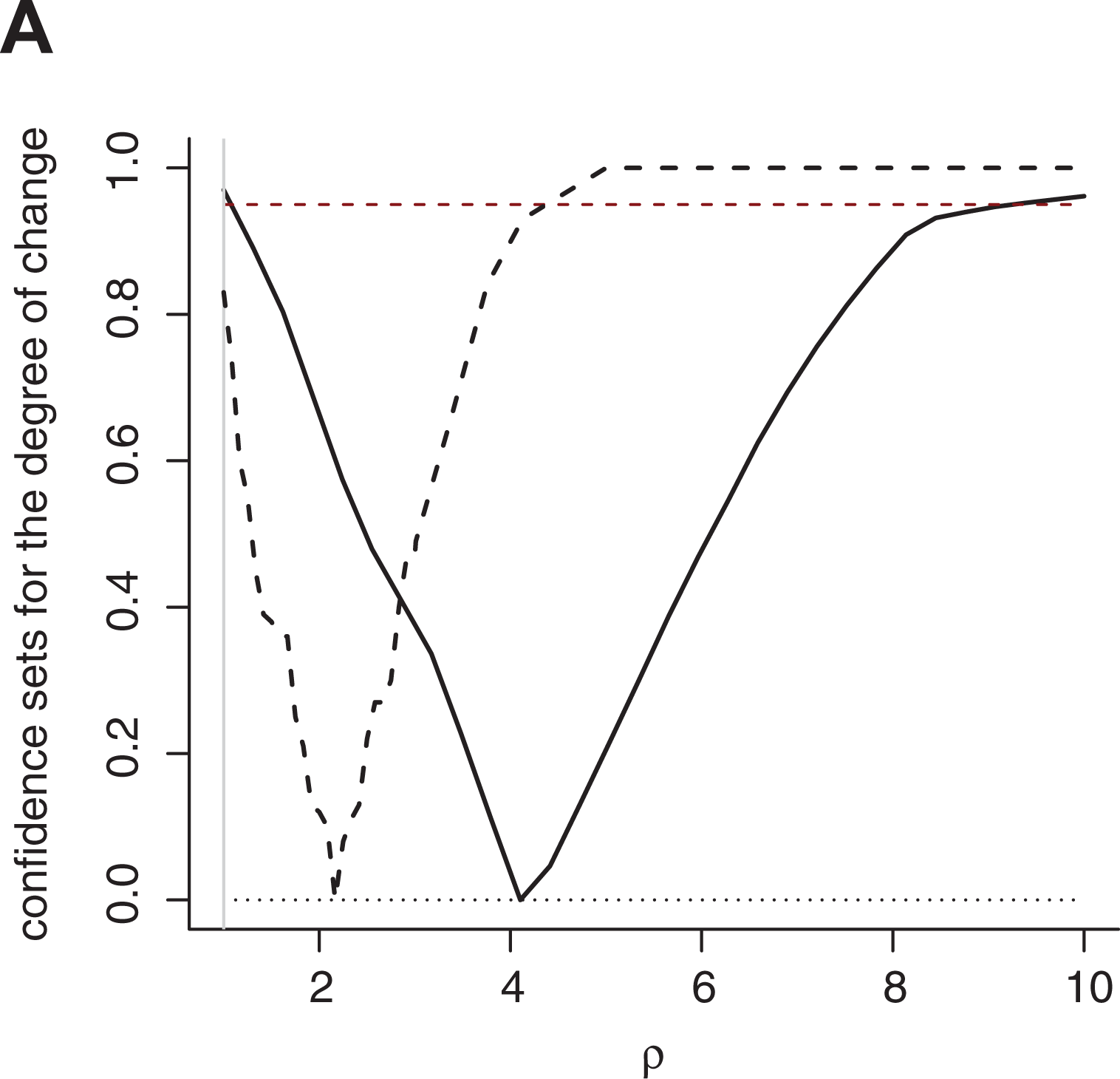
Figure 4A gives the confidence curves for the two degree of change parameters described above. These are computed with the simulation based method described in Section C of the Online appendix. The confidence curves reveal that the ratio between upper quartiles is significantly larger than 1 on the 95% level, whereas the ratio of medians is larger than 1 only at somewhat lower confidence levels. Thus, the upper quartiles on each side of the potential change-point are significantly different on a 5% level. This analysis is not conditional on a given change-point value, but takes into account the uncertainty in the change-point position.
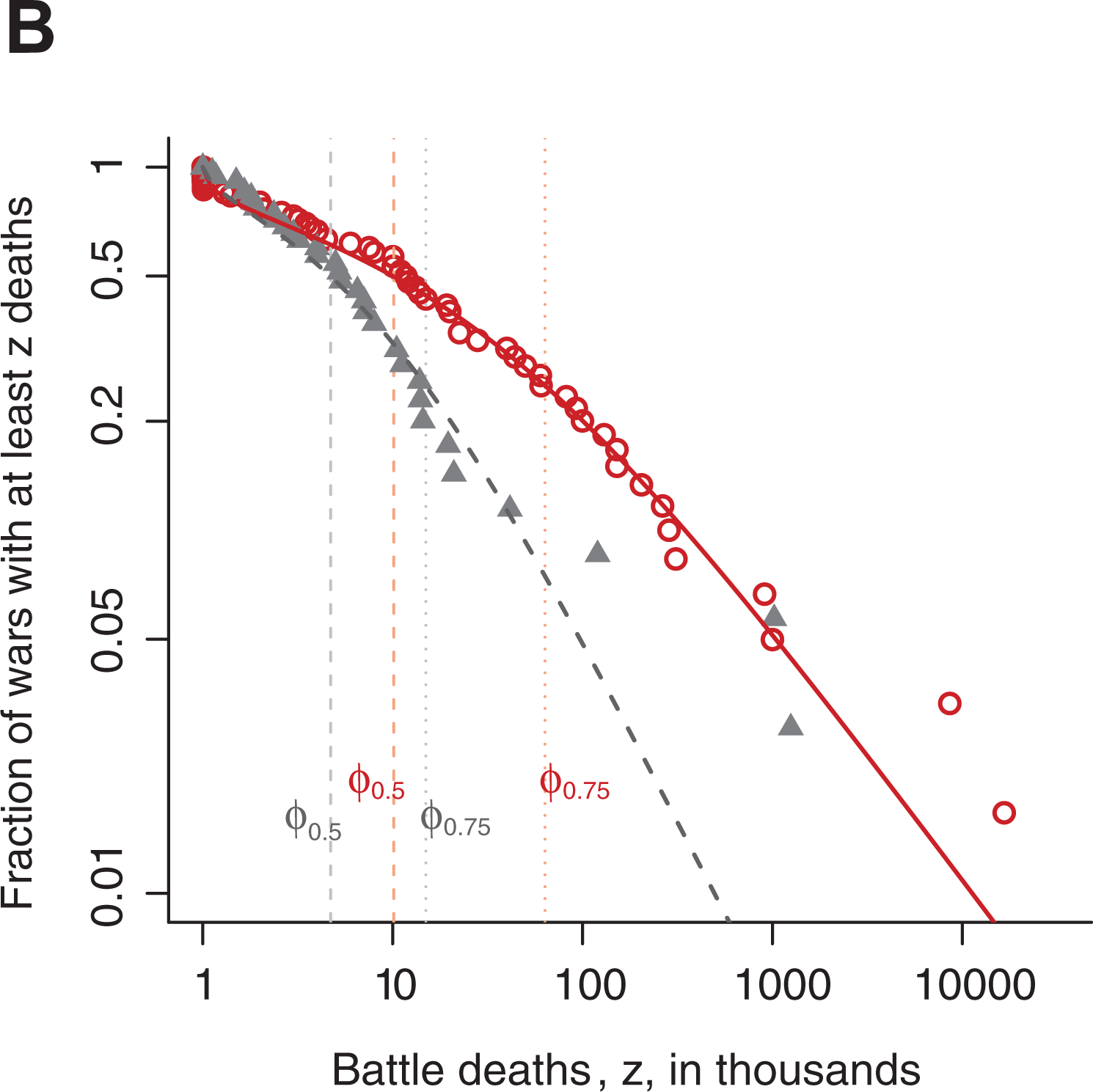
Figure 4B gives a different way to visualize the change in distribution at the estimated change-point. The red dots are wars taking place before the Korean war, and the black dots are the wars after. The lines are the fitted complement cumulative distribution functions (CDFs), That is, 1 minus the fitted CDFs, on the log-log scale for the inverse Burr distribution on each side of the estimated change-point. The vertical dashed lines indicated the fitted medians and upper quartiles, and again we observe that the difference between the two distributions is larger for the higher quantiles. We also see that for Confidence curve for the change-point using the inverse Burr model Confidence curves for the degree of change, using the inverse Burr model log-log plot of the complement CDFs for war sizes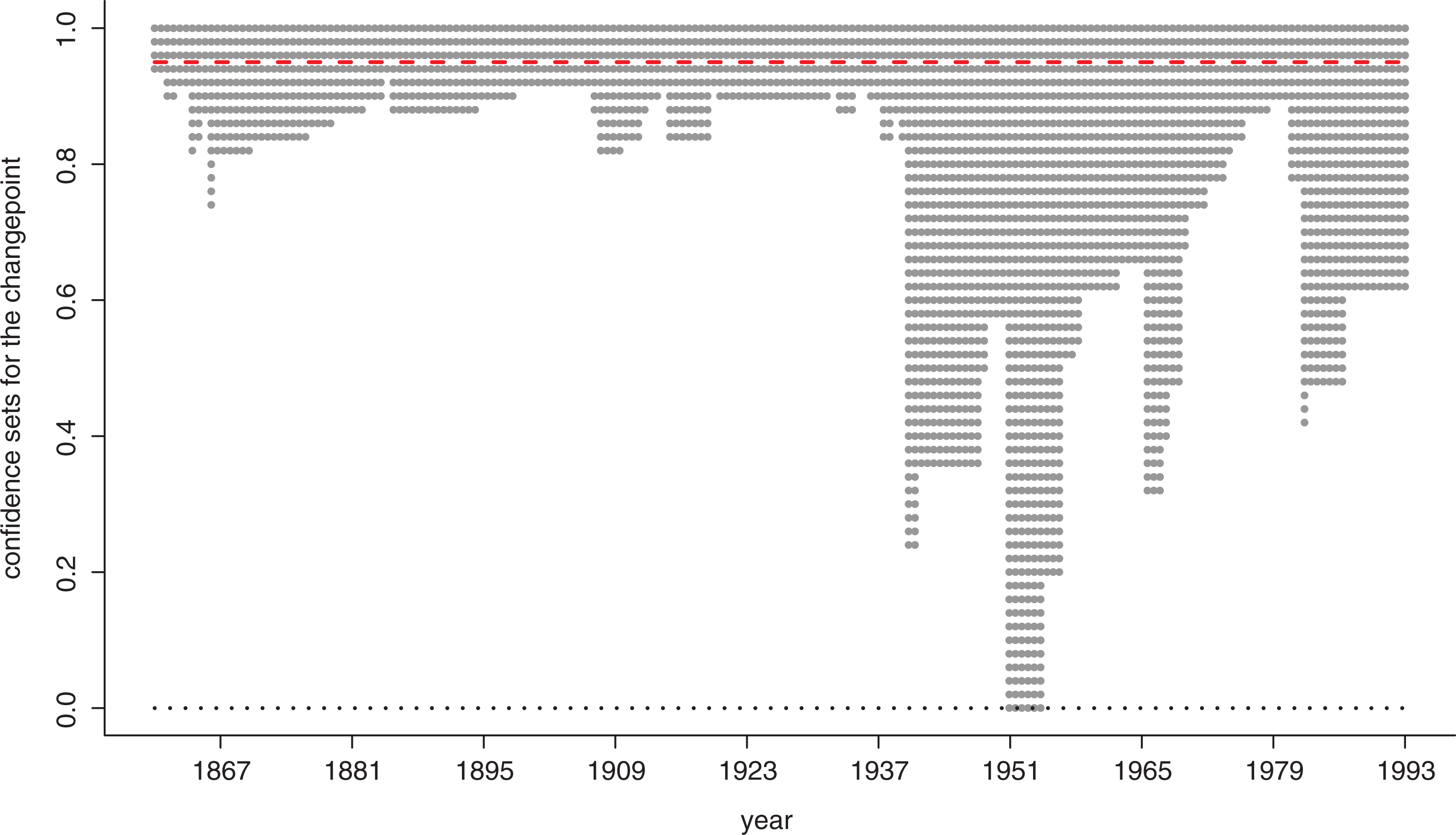
Covariate results
We include the democracy covariate and allow the effect of democracy to change across the change-point. The inclusion of the covariate changes the point estimate of the change-point somewhat, from 1950.483 to 1967.431 (the Six Day war). The Korean war is still given high confidence and we have therefore performed follow-up analysis taking the 1950.483 change-point as given. When it comes to parameters Regression with inverse Burr model and mean democracy as covariate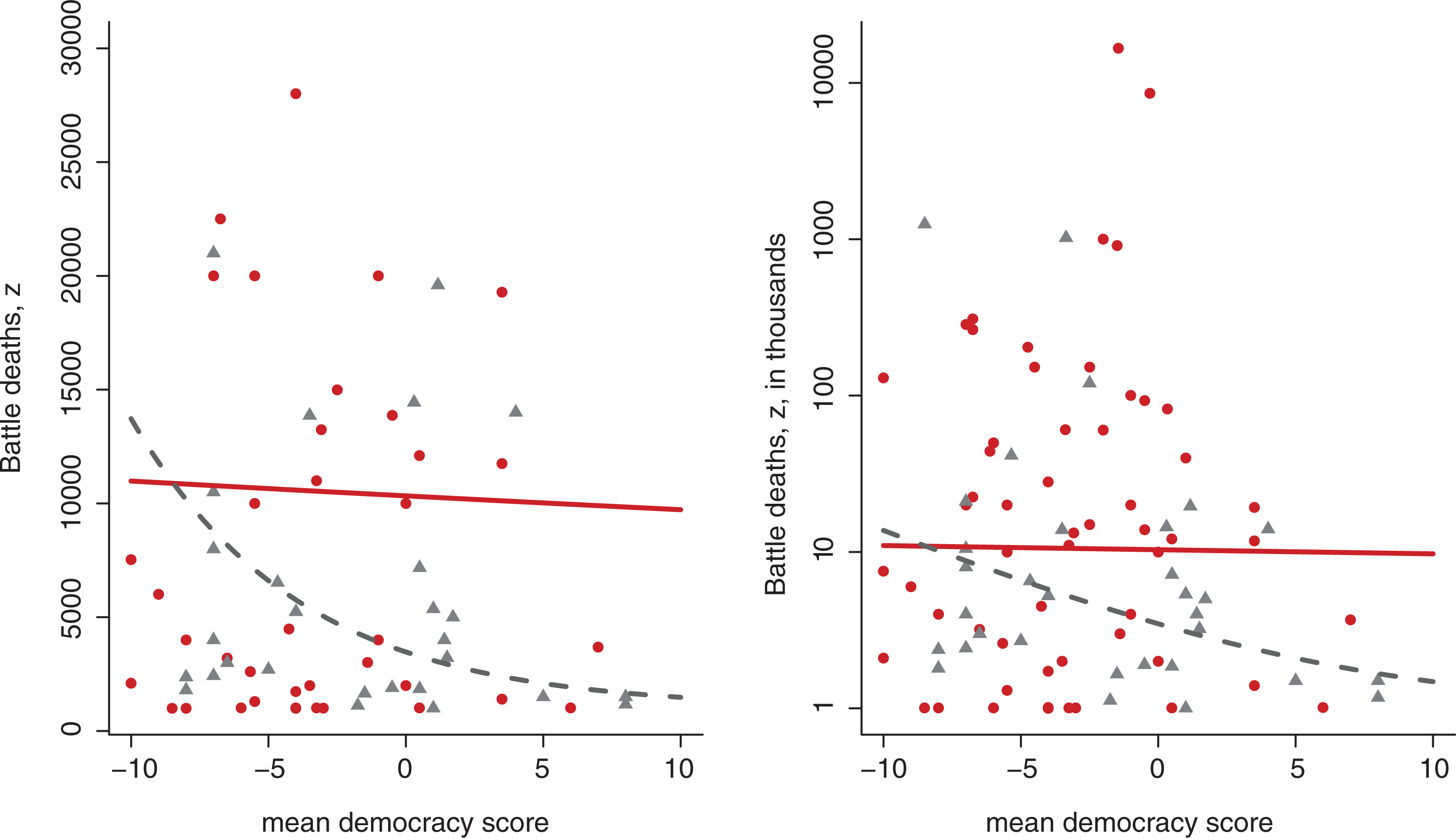
Discussion
Recent contributions, reviewed above, argue that there is no clear evidence of change in the sizes or the times between interstate wars since 1816. In contrast, we find evidence that a change in the distribution of war sizes has taken place, and that it may have happened in the years after WWII, rather than in 1945 which is the assumed change-point within the current literature. We stress that the results from the change-point analysis are open to interpretation. On one hand there is considerable uncertainty in the change-point position: the 95% interval for τ covers the entire range of possible change-point positions. Some readers will thus interpret Figure 3 as favouring the ‘no-change’ hypothesis. On the other hand, the figure also indicates that all the most likely candidates for the change-point positions are found either at or after WWII. Moreover, the degree of change analysis shows a significant decrease in battle-deaths after the change, at least when considering the upper quartiles. The change in the parameters of the distribution of battle-deaths thus manifests itself in smaller wars in the period after the change-point. On the whole, we interpret our analyses as supporting a decrease in battle-deaths at some point in the time span we are considering. The exact position of the shift remains somewhat uncertain, but the most likely candidate is the Korean war.
Our claim rests upon two distinct analyses. First, we presented a non-parametric test of homogeneity. The test suggests that the sequence of war sizes has not been homogeneous when considering the higher quantiles of the war size distribution; see the results for the upper quartiles in Figure 2. With this test the null hypothesis of no change is rejected at the 5% level. Second, we have conducted a change-point analysis. Here, we needed a parametric model for the data, and we found suitable models among the class of models with power law tails.
We have also introduced the use of covariates – pointing towards further modelling efforts including mechanisms and explanations. In addition to enriching the long peace debate by generating hypotheses concerning the long-term characteristics of interstate wars, we have also introduced models and methods to the peace research literature. In the rest of this section, we will discuss our findings on various levels. First, we will take a critical look at our approach and report on some robustness checks we have conducted. Then we will explore connections between our contribution and related articles, both in terms of methods and results. Finally, we will discuss our findings in light of the general peace research literature, and in particular consider some theoretical explanations.
Robustness of our approach
Statistical analyses require a series of assumptions and some level of abstraction to get from a real world question to a statistical question. Here, we return to some of the choices we discussed in the beginning and attempt to assess their influence on our results.
For our statistical modelling we have been guided by previous works using power law distributions. There have been a few attempts to give a theoretical justification to the power law behaviour of war sizes (see e.g. Cederman, 2003), but for most authors, including Richardson, the power law models have been used as essentially descriptive models, that is, as ‘lower dimensional representations’ allowing us to assess potential regularities given the inherent variation in the data. In that case, it is particularly important that the model fits well to the data – that the distribution of war sizes according to the model is close to the actually observed war size distribution. We have therefore conducted various goodness of fit evaluations, for example the log-log plot in Figure 4. We see that the data in general have a good fit to the inverse Burr models on each side of the change-point. The clearest deviation from the model is found for the very largest wars, especially among those taking place after 1950. The three largest wars in this period have more battle-deaths than expected under the model. This particular aspect of the data was not successfully accounted for by any of the models we considered (see the corresponding figures in the Online appendix) and would necessitate a more complex model than those considered so far. We have also conducted some goodness of fit tests. On both sides of 1950, the observed data were consistent with having been generated by the fitted inverse Burr distributions (
Several models within the class of distributions with power law tails provide adequate fit to the data. In order to investigate the sensitivity of our results to the modelling assumptions, we present results for similar change-point analyses assuming two different models for the data in the Online appendix: the simple power law distribution and the inverse Pareto distribution. The inverse Pareto, like the inverse Burr, models the full sequence of 95 war sizes, and we obtained very similar results to those presented in Figures 3 and 4: the same point estimate for the change-point,
The different estimated change-points, for the full battle-deaths distribution and only the large wars (the simple power law analysis), underscores an important aspect inherent to any change-point exercise. What constitutes a change-point when analysing some aspects of the available data will not necessarily be recognized as a change-point when examining other relevant data. Thus it should not be seen as a paradox that the Vietnam war in 1965 can be a change-point for the extreme tail of the battle-death distribution, whereas perhaps the Korean war in 1950 is more of a change-point when examining more complex models involving the full battle-death distribution.
Some readers might question our choice of using a change-point framework at all. As mentioned in the beginning, change-point methods assume a very particular form of change, an abrupt shift in the distribution generating the data. In the case of our change-point method, we have in addition assumed that only a single such shift takes place. Is it realistic to assume that the long peace emerged in that way? Hardly, but a single change-point model could be considered a reasonable approximation to various other patterns, for example to more gradual changes. We are inclined to interpret the change-points we identify here as the culmination of a process that has unfolded over some time. This could apply to several of the mechanisms discussed below.
Connections to other analyses
There are several recent contributions with clear connections to our article. Many of these also analyse the CoW interstate conflict dataset (Clauset, 2017, 2018; Spagat & van Weezel, 2018; Fagan et al., 2018; Braumoeller, 2019), while Cederman, Warren & Sornette (2011) and Cirillo & Taleb (2016) use datasets with a longer time span (from year 1494, and year 1, respectively). Cirillo & Taleb (2016) and Spagat & van Weezel (2018) normalize the war sizes with respect to world population, while Clauset (2017, 2018) and Cederman, Warren & Sornette (2011) analyse the absolute numbers. Fagan et al. (2018) conduct analyses of both absolute and relative numbers. As expected, analyses using relative war sizes find a clearer decline of war than those focusing on absolute numbers.
Parametric models within the class of distributions with power law tails are used in Cederman, Warren & Sornette (2011), Cirillo & Taleb (2016) and Clauset (2017, 2018), while Fagan et al. (2018) and Spagat & Weezel (2018) use non-parametric approaches. Clauset (2017, 2018) also investigated a certain semi-parametric model. The articles also differ in their choice of framework for investigating potential trends. Cirillo & Taleb (2016) and Clauset (2017, 2018) use types of homogeneity tests. Spagat & van Weezel (2018) test for differences in the probability of observing wars of a certain size across specific potential years-of-change, namely 1945 and 1950. Initially, Cederman, Warren & Sornette (2011) also investigate a single, specific year-of-change, 1789, but the authors proceed by searching for a change-point along the full sequence of wars. Their approach differs from ours: they do not make use of a formal change-point method and their method does not provide any measures of uncertainty. Fagan et al. (2018) use a formal change-point method based on work by Killick, Fearnhead & Eckley (2012) and Haynes, Fearnhead & Eckley (2017), but their approach has several differences from ours. Their methodology relies on an algorithm which introduces distributional changes in the data sequence when the change-point leads to a sufficiently large increase in the fit to the data. The fit is measured by some cost function, which the user has to define, along with some penalty function (against introducing unnecessary change-points). In contrast, our change-point method treats the change-point as a parameter in the model and we therefore analyse it in a parallel manner as we would ordinary model parameters. Our method also allows investigating the magnitude and direction of the change, which Fagan et al. (2018) do not provide. On the other hand the method in Fagan et al. (2018) naturally allows for multiple change-points, while we have only investigated the introduction of a single potential change-point.
As mentioned in the beginning, Cirillo & Taleb (2016) and Clauset (2017, 2018) test a null hypothesis of stationarity, and do not find sufficient statistical evidence to reject it. Cederman, Warren & Sornette (2011) find a shift towards larger wars in 1789, while Spagat & van Weezel (2018) find a shift towards smaller wars after 1950. Fagan et al. (2018) find multiple change-points in the sequence of wars between 1816 and 2007, notably around 1950. Braumoeller (2019), using a non-parametric change-point model, finds no change-point in war intensity – measured as battle-deaths per combatant population – or in war severity – measured as total battle-deaths. Braumoeller (2019) does find a change-point in the rate of which wars are initiated, but if anything this indicates that the Cold War period was more not less warlike than other periods.
How can all these results be reconciled with each other, and with ours? First of all it is important to realize that they do not necessarily stand in stark opposition to each other. The studies differ in the time span considered and in the specific research question they treat, through their choices of, for example, normalization and statistical framework. Also, as usual, non-rejections do not imply that the null hypothesis is true. Further, the homogeneity tests used in Cirillo & Taleb (2016) and Clauset (2017, 2018) differ from the one we use. The test in Clauset (2017, 2018) investigates whether the observed dataset as a whole is sufficiently different from simulated data from a stationary model. Our test focuses on specific aspects of the distribution of the data, specifically the upper quartile for instance. This sharper focus likely increases the statistical power. This focus is also shared by our degree of change investigations where we study changes in the medians and upper quartiles.
There is no clear consensus among the studies mentioned here, but neither is there any strong incompatibility, despite the differences in methodology. Each should be considered as providing some evidence to the full picture, which remains to be fully understood. In further work, we hope to draw on these studies and devote energy into the development of more realistic models for the underlying processes behind the war characteristics we observe, incorporating explicit theoretical mechanisms.
Mechanisms
So far, we have not discussed the mechanisms that may underlie the patterns our analysis has revealed. In this, our exercise is similar to the path-breaking work of Richardson (1960) and the aforementioned articles by Clauset (2018, 2017), Cirillo & Taleb (2016) and Fagan et al. (2018), which mainly focus on modelling battle-deaths and uncovering potential trends. 2 A full investigation of mechanisms is beyond the scope of this article. Nonetheless, we will discuss a set of plausible mechanisms that could help explain the change-point our analysis revealed. We base this discussion on existing theoretical work.
There exists a large literature attempting to explain the production of wars at the systems level. Of particular relevance are the contributions by Cederman and co-authors. Cederman (2003) builds an agent-based model for war and state formation that reproduces the power law distribution of war. He argues that ‘technological change and contextually activated decision-making go a long way toward explaining why power laws emerge in geopolitical systems’ (Cederman, 2003: 147). As mentioned above, Cederman, Warren & Sornette (2011) find a change-point in 1789, with a subsequent increase in the severity of war. They discuss potential explanations driving the shift, and argue that it was driven by a revolution in the technology of statecraft, especially in the ability of states to extract resources and organize their militaries.
Our analysis identified 1950 and the Korean war as the most likely change-point in the distribution of battle-deaths in international wars. A change-point in the period around and following the Korean war fits well with the thesis developed by Pinker (2011: Ch. 5). Here the mechanism underlying the change-point would be the cultural, political and moral shift that took place across especially the Western world. War went from being an appropriate part of statecraft, ‘the continuation of policy by other means’ (Clausewitz, 1989), to something inappropriate or even evil (Mueller, 1989). This shift began in the post-Korean war world, and is particularly associated with the Vietnam war period. As informal evidence for the argument Pinker (2011) lists a multitude of songs and movies from that period with clear and explicit anti-war themes, themes that were much less present in earlier periods.
In addition to this norms-based mechanism, we consider two other mechanisms particularly plausible. The first centers around the development of nuclear weapons. When the USSR conducted its first atomic weapons test in 1949, the two superpowers, the USA and the USSR, created the basis by which war could escalate to a point where the world would face total annihilation. The development of the system of mutual assured destruction led all key actors to fear that low intensity conflict could escalate into thermonuclear war (Kahn, 1965). This restraining effect could operate as a mechanism reducing the intensity of international conflicts. We could label this the ‘George Orwell Mechanism’. In his essay ‘You and the Atomic Bomb’ (October 1945), Orwell predicted that power would be consolidated in the hands of the superpowers due to the atomic bomb, and that these two would perpetually threaten atomic war against each other, without actually risking it. As a result, large-scale wars would end and instead we would see the rise of a new form of smaller wars. The restraining effect of nuclear weapons could by itself be an important mechanism, but this mechanism may have been further strengthened by the system of international governance, and especially the United Nations, which was developed to help defuse conflicts before they escalated out of control (Goldstein, 2011).
A second mechanism centers around the role of democracy. Democracies very rarely go to war against each other, a tendency labelled the democratic peace (see e.g. Maoz & Russett, 1993). Moreover, Mitchell, Gates & Hegre (1999) show that the relationship between democracy and war has become more pronounced over time, indicating that democracy could be particularly useful for studying change-points in the history of interstate wars. In the section ‘Covariate results’ in this article, we do indeed find an increasingly pacifying effect of democracy, though this analysis is only indicative, and the results should be treated with caution. In the period before 1950, democracy seems to have no effect on the number of battle-deaths. After 1950, however, the wars between more democratic countries have become much less violent. The increasing effect of democracy on conflict coupled with a simultaneous increase in the number of democracies in the world could translate into a more peaceful world in the aggregate.
Supplemental Material
Supplemental Material, SDI896843_appendix - Statistical sightings of better angels: Analysing the distribution of battle-deaths in interstate conflict over time
Supplemental Material, SDI896843_appendix for Statistical sightings of better angels: Analysing the distribution of battle-deaths in interstate conflict over time by Céline Cunen, Nils Lid Hjort and Håvard Mokleiv Nygård in Journal of Peace Research
Footnotes
Replication data
Acknowledgements
We appreciate comments from Aaron Clauset, Jens Kristoffer Haug, Steven Pinker and Michael Spagat. We are also very grateful for the detailed and constructive comments from three anonymous reviewers.
Funding
We are grateful to the NRC funded five-year project FocuStat, and to several of its participants for active discussions, in particular Gudmund Hermansen and Emil Stoltenberg, and to the NRC funded ‘Young Research Talent’ project MiCE (project no. 275400).
Notes
References
Supplementary Material
Please find the following supplemental material available below.
For Open Access articles published under a Creative Commons License, all supplemental material carries the same license as the article it is associated with.
For non-Open Access articles published, all supplemental material carries a non-exclusive license, and permission requests for re-use of supplemental material or any part of supplemental material shall be sent directly to the copyright owner as specified in the copyright notice associated with the article.