Sage Journals: Discover world-class research

Abstract

Using the latest spatial econometric techniques and data pertaining to 144 countries over the period 1993–2007, this article tests and compares four frequently used spatial econometric models and eight matrices describing the mutual relationships among the countries, all within a common framework, which helps clarify the impact of neighboring countries on military expenditures. Furthermore, it utilizes two different data sources. Due to this setup, it provides one of the most thorough spatial analyses of military expenditures so far. Furthermore, it confirms but also challenges the results of several previous studies. Military spending measured as a ratio of GDP in one country indeed depends primarily on the spending of other countries, but in a limited number of cases, it also depends on control variables that can be observed in other countries, among which are the level of GDP, the occurrence of international wars, and the political regime. The most likely specification of the matrix describing the relationships among countries is the first-order binary contiguity matrix based on land or maritime borders, extended to include two-sided relationships among the five countries that are permanent members of the UN Security Council and one-sided relationships to all other countries. Finally, cross-sectional approaches are rejected in favor of dynamic spatial panel data approaches due to their controls for habit persistence, country, and time-period fixed effects.

Keywords

country spillovers defense burden military expenditures spatial interaction

Introduction

As noted by Collier & Hoeffler (2007) and many others, the need for security is a crucial reason for spending scarce government budgets on military force. Security is difficult to quantify though, but models of arms races (Richardson, 1960) and alliances (Sandler & Hartley, 2001) suggest that security is influenced by the military expenditures of the country itself and that of other countries. In particular, there is a large literature devoted to trying to explain the logarithm (log) of the ratio of the military expenditure of a country to its gross domestic product (GDP), often called the defense burden. This will be determined by the defense burden in neighboring countries, and possibly other variables in these countries. These co-determinants in the dependent variable, the explanatory variables, and/or the error term from neighboring countries are called spatial lags following the spatial econometrics literature, a growing subfield in econometrics dealing with spatial interactions among geographical units, in this case countries. Two crucial issues involved in specifying a spatial econometric model are the choice of the type of spatial lags and the choice of a weight matrix that specifies who a country’s neighbors are. Up to now most studies only consider one type of spatial lag and do not test different weight matrices against each other. Additional but non-spatial issues are whether or not to control for habit persistence, whether to take the defense burden or the level of military expenditures as the dependent variable, and whether country and time fixed effects need to be controlled for. These issues are introduced in the next section.

The objective of this study is to establish a rationale for the different spatial lags and spatial weight matrices, apply a testing procedure that can identify which types of spatial lags in combination with which type of spatial weight matrix best fit the data, and provide a clearer understanding of the impact of neighboring countries on military expenditure. Accordingly, this study considers four spatial econometric models specifications and eight potential specifications of the spatial weight matrix in an empirical analysis. Using a Bayesian comparison approach developed by LeSage (2014, 2015), we test these 32 (4 × 8) combinations within a common framework.

As the theoretical background for extending empirical models of military expenditures with spatial lags, and to place the results into perspective, we also present a simple economic model. Departing from a neo-classical welfare model that makes security an integral component (Smith, 1989, 1995), we extend the security function to include the military expenditures and economic, political, and strategic factors that mark other countries (Brueckner, 2003). In addition, we test for the existence of country spillover effects, defined as the marginal impact of a change in one explanatory variable in country j on the defense burden or military expenditures of country i (i ≠ j). These spillover effects can be derived from the reduced form of a spatial econometric model (we provide mathematical details in the next section) and offer useful additions to the direct effects that measure only the marginal impact on the dependent variable pertaining to the focal country itself.

In the next two sections, we detail our spatial econometric methodology for military expenditure contexts, together with the basic economic-theoretical background explanation for spatial lags. After introducing the explanatory variables, data and sources, and the different spatial weight matrices being examined, we present the results of our empirical analysis. The final section concludes.

Spatial lags and weights

Basically, there are three main types of spatial lags that can be used to explain the defense burden of a country (LeSage & Pace, 2009; Elhorst, 2014). First, an endogenous spatial lag measures whether the defense burden of country i depends on the defense burden of other countries j (j ≠ i), or vice versa, resulting in the spatial autoregressive (SAR) model that appears in several studies. For example, Quiroz Flores (2011) uses cross-section data from the World Bank (WB) to explain the defense burden indicator across 168 countries in the year 2000. Goldsmith (2007) also uses cross-section data, in this case from 129 countries in 1991 extracted from the Correlates of War (COW) project, but also anticipates that the indicator depends on the value observed in the previous year, which helps control for habit persistence. Finally, Skogstad (2016) employs time-series cross-section data, or a spatial panel, related to 124 countries over a period of 16 years (1993–2008) from the Stockholm International Peace Research Institute (SIPRI). Panel data allow one to control for country- and time-specific effects (Baltagi, 2004).

Second, a spatial lag among the error terms might be pertinent if countries share similar unobserved characteristics or face similar unobserved institutional environments. Models that rely on this lag are known as spatial error models (SEM), but they remain rather unpopular. As Beck, Gleditsch & Beardsley (2006: 30) explain, ‘The spatial lagged error model is odd (at least in many applications), in that space matters in the “error process” but not in the substantive portion of the model.’ Goldsmith (2007: 422) examines the plausibility of SEM in addition to the SAR model, but only as a ‘first-cut of the topic’.

Third, exogenous spatial lags can measure whether the defense burden of country i depends on the explanatory variables of other countries j (j ≠ i). If the number of explanatory variables is K, the maximum number of lags of this type is also K. Models containing these lags take the designation of a spatial lag of X (SLX). Although exogenous spatial lags are widely used, they are less common in the context of spatial econometric models. One exception is Phillips (2014) who relies on an unbalanced spatial panel of 135 developing countries taken from the COW project over the period 1950–2006 to investigate whether a country bordering a civil war zone spends more on military expenditures than a country that is not in such a situation.

Accordingly, K + 2 spatial lags are possible. In addition to the SAR, SEM, and SLX models with one type of spatial lag, alternative models combine two or even three types of spatial lags. We introduce these combination models in the section on spillovers.

Another crucial issue for explaining military expenditures using variables observed in other countries is determining which set of countries might affect the focal nation. Generally, mutual relationships among countries are modeled by the so-called spatial weight matrix W, whose elements can depend on geographical, economic, or political distances between countries. Goldsmith (2007) explores two specifications: a binary contiguity matrix based on land or maritime borders and an inverse distance matrix based on the great circle distance between the capital cities of countries. Skogstad (2016: 33) includes three additional specifications, based on whether countries have ‘the ability to project their military power worldwide’, and Quiroz Florez (2011) uses two principles to construct seven potential specifications. For example, if the geographical distance between the capital cities between countries is less than cut-off points of 1,000, 2,000, 4,000, or 8,000 km, the countries might be assumed to be neighbors. A second principle is based on alliance membership.

As these various approaches imply, one of the biggest problems in empirical spatial econometric research is choosing among different model specifications and specifications of W. Too many studies only consider one type of spatial lag, resulting in just an SAR, SEM, or SLX model, without testing model specifications against one another or considering potential extensions that include additional types of spatial lags. The endogenous spatial lag offers a well-accepted explanation of the military defense burden that is embedded in economic-theoretical literature (as detailed further in the section on theory), but its impact might be overestimated, whether due to the omission of exogenous spatial lags or of country- and time-specific effects, as demonstrated by Corrado & Fingleton (2012) and Lee & Yu (2010) using Monte Carlo simulations. In an effort to advance this research stream, we consider combinations of different types of spatial lags, test the model specifications against one another, and determine whether country- and time-specific effects are jointly significant.

A related issue is the choice of the spatial weight matrix. The aforementioned studies consider different specifications of this matrix, so this choice is of crucial importance. However, none of the cited studies test the suggested specifications against one another. Generally, they present and discuss the results for the different specifications mainly to check whether they are robust to the choice of the specification; they do not identify which specification is most likely.

Spatial model of military expenditures

A spatial econometric model is a linear regression model extended to include spatial lags in the dependent variable, the explanatory variables, the error term, or some combination thereof. Including all spatial lags yields a so-called general spatial nesting model

D_{t} = ρ W D_{t} + X_{t} β + W X_{t} θ + μ + ξ_{t} + u_{t}

u_{t} = λ W u_{t} + ∊_{t}

where D_t denotes an N × 1 vector of the log of the defense burden indicator, that is, military expenditure (M) as a ratio of GDP (Y) for every country (i = 1,…, N) in the sample during time period t (t = 1,…, T); X_t is an N × K matrix of exogenous explanatory variables associated with the K × 1 vector β; W is an N × N non-negative spatial weight matrix describing the neighbors of a country, whose diagonal elements are 0 because a country cannot be its own neighbor; and WD_t represents the endogenous spatial lag, WX_t the exogenous spatial lags, and Wu_t the spatial lag among the error terms. The scalars ρ and λ, as well as the K × 1 vector of parameters θ, measure the strength of these spatial lags. Furthermore, μ is a vector of country fixed effects, ξ_t is a time fixed effect, and ε_t is a vector of error terms. Whether we should include country and time fixed effects is a question to be tested.

Theory

The rationale for this spatial econometric model derives from Smith (1989, 1995) and Brueckner (2003). According to Smith, nation states can be represented as rational agents that maximize a social welfare function U_i depending on security S_i and civilian output C_i:

U_{i} = U (S_{i}, C_{i})

Other studies also depart from a social welfare model (e.g. Collier & Hoeffler, 2007; Dunne & Perlo-Freeman, 2003a,b; Nordhaus, Oneal & Russett, 2012). Maximizing the social welfare function is subject to a budget constraint on military spending and a security function that determines security in terms of the country’s own and other countries’ military forces. The budget constraint takes the form:

Y_{i} = P_{c} * C_{i} + P_{m} * M_{i}

where Y_i represents the national income or GDP of country i, and P_c and P_m are the prices of civilian output C_i and real military spending M_i. According to Smith (1995), security, similar to utility or welfare, is unobservable and thus can be measured by the military expenditures of the country, in combination with other economic, political, or strategic variables, denoted X_i. Following literature on strategic interactions among governments (see Brueckner, 2003), the level of security in a particular country also depends on the military expenditures of other countries and their economic, political, and strategic variables. For example, the (perceived) security of a country might diminish if a neighboring country increases its military expenditures, gets involved in an international or civil war, or undergoes a political regime change (we explain these variables in more detail in the next section). If WM_i and WX_i denote the counterparts of M_i and X_i observed in neighboring countries, we can formalize the security function as:

S_{i} = S (M_{i}, W M_{i}, X_{i}, W X_{i})

Maximizing the social welfare function in Equation (2), subject to the budget constraint in Equation (3) and the security function in Equation (4), yields the following military expenditure demand function:

M_{i} = M (W M_{i}, Y_{i}, W Y_{i}, X_{i}, W X_{i})

which represents a reaction function – that is, country i’s best response to the choices of other countries regarding their military expenditures, income levels, and other control variables.

The magnitude of the slope of this reaction function, represented by the spatial autoregressive parameter ρ in Equation (1), is of interest for the current study. According to Goldsmith (2007), this magnitude depends on three factors. First, in Richardson’s (1960) classical arms race, the greater a country’s arms stock, the greater its neighbors’ stocks will be. Second, alliances might mitigate this factor, because a state with a high stock may be surrounded by neighbors with low stocks, and a 0 coefficient occurs because its arms stock has no effect on the stocks of its neighbors. In this scenario, a nation is not alarmed when neighboring countries increase their arms stocks, and no spiraling arms race is initiated. When several neighboring countries form an alliance, some members might even avoid making additional investments in defense or cut back their defense expenditures, in a form of free-riding behavior (Sandler & Hartley, 2001). Third, if a country can distinguish offensive from defensive arms build-ups by its neighbors, several countries may maintain minimal defensive forces, as long as no offensive action takes place.

Dynamics

In addition to a static model, Goldsmith (2007) considers a dynamic version that includes the temporal lag of the dependent variable, D_t– ₁, to control for habit persistence. That is, military expenditure measured by the defense burden indicator is subject to budgetary inertia because spending depends on decisions made in previous periods and might be subject to bureaucratic institutions (DiGiuseppe, 2015). According to Goldsmith, the coefficient of this variable was 0.802 when using distance weights and 0.715 when using contiguity weights; for DiGiuseppe, it ranged from 0.852 to 0.997. In both studies, the coefficient was highly significant (1% level). Beck, Gleditsch & Beardsley (2006) also discuss the possibility of including a one-period lag in the spatially lagged dependent variable, which may be denoted WD_t– ₁. Korniotos (2010) applies this model to explain annual consumption growth in US states during the period 1966–98 and interprets the coefficients of the temporal and space-time lags of the dependent variable as measures of the relative strength of internal and external habit persistence. This extension reads as

D_{t} = τ D_{t - 1} + ρ W D_{t} + η W D_{t - 1} + X_{t} β + W X_{t} θ + μ + ξ_{t} + u_{t}, and

u_{t} = λ W u_{t} + ∊_{t}

also known as the dynamic general spatial nesting model (Firmino Costa da Silva, Elhorst & da Mota Silveira Neto, 2017). Yildrim & Öcal (2016) use this model to explain the impact of military expenditures on economic growth.

Expenditures and defense burden

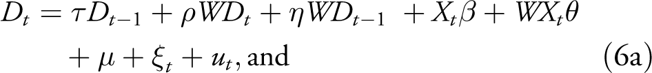
Some discussion in prior literature pertains to whether to employ the log of a state’s military expenditure while controlling for its economic size or the ratio of a state’s military expenditure to its GDP (see DiGiuseppe, 2015). When two countries are of comparable size (e.g. United States and Russia; Namibia and Angola), one country likely adjusts its defense burden to match that of the other country. However, if the sizes of two neighboring countries vary more substantially (e.g. United States and Mexico), this adjustment mechanism seems unlikely. The impact of an increase in M in Mexico on that of the United States likely differs from the impact of an increase in M in the United States on that of Mexico. 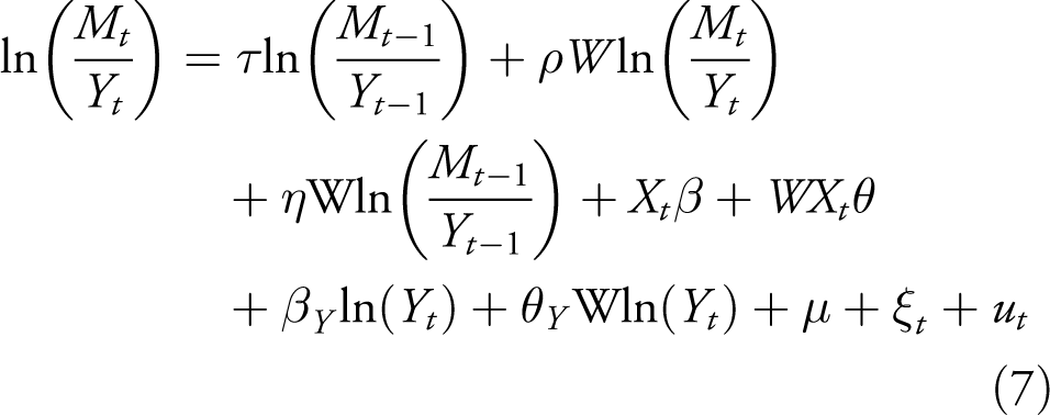We can rewrite Equation (5) as $\frac{M_{i}}{Y_{i}} = M (W \frac{M_{i}}{Y_{i}}, Y_{i}, W Y_{i}, X_{i}, W X_{i})$ ; similarly, Equation (1a) can be rewritten as

ln (\frac{M_{t}}{Y_{t}}) = τ ln (\frac{M_{t - 1}}{Y_{t - 1}}) + ρ W ln (\frac{M_{t}}{Y_{t}}) + η Wln (\frac{M_{t - 1}}{Y_{t - 1}}) + X_{t} β + W X_{t} θ + β_{Y} ln (Y_{t}) + θ_{Y} Wln (Y_{t}) + μ + ξ_{t} + u_{t}

where the economic size of a country denoted by Y is separated from the other explanatory variables X, the notation ‘ln’ indicates that military expenditures and the level of GDP are expressed in natural logarithms, and the (natural) log ratio between M and Y serves as the dependent variable.¹ Then we can rewrite Equation (7) as

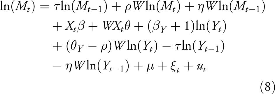
ln (M_{t}) = τ ln (M_{t - 1}) + ρ W ln (M_{t}) + η W ln (M_{t - 1}) + X_{t} β + W X_{t} θ + (β_{Y} + 1) ln (Y_{t}) + (θ_{Y} - ρ) W ln (Y_{t}) - τ ln (Y_{t - 1}) - η W ln (Y_{t - 1}) + μ + ξ_{t} + u_{t}

showing that the spatial autoregressive coefficients ρ and η reflect both the impact of the ratio of military expenditure to GDP observed in neighboring countries at time t and t–1 on that of the focal country (Equation (7)) and the impact of the level of military expenditure observed in neighboring countries on that of the focal country (Equation (8)). The same principle applies to the coefficients β and θ of the X and WX variables. Only with respect to the GDP variable is there a notable difference. If β_Y = 0 in Equation (7), then in Equation (8), the level of military expenditure increases proportionally with its level of GDP in the short term; it increases less than proportionally if −1 < β_Y < 0 and more than proportionally if β_Y > 0. One issue (raised by one reviewer) is whether temporal lags of GDP (ln(Y_t) and Wln(Y_t−1)) should also be included. We test this by showing what happens if the coefficients of these variables are set to zero.²

To further understand the impact of GDP observed in neighboring countries, we also need to introduce direct and spatial spillover effects.

Spillovers

Spatial econometric models often focus on country spillover effects, such as whether a change to the level of GDP in a particular country affects the defense burden ratio or level of military expenditures in neighboring countries. Comparisons of point estimates, such as those derived from non-spatial models that do not account for spatial lags in neighboring countries, with the findings of spatial econometric models, or of different spatial econometric models mutually, may lead to erroneous conclusions. As LeSage & Pace (2009) demonstrate, a partial derivative interpretation can offer a more valid basis for testing this hypothesis, but only for cross-sectional data. Departing from a dynamic general spatial nesting model based on spatial panel data, Elhorst (2014) shows that the matrix of partial derivatives of the expected value of the dependent variable with respect to the kth independent variable for i = 1,…, N is given by the N ×N matrix,

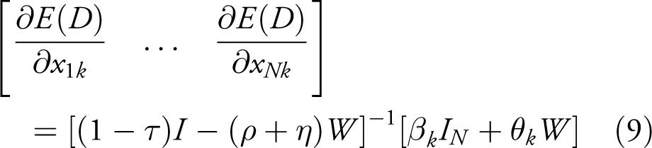
[\begin{matrix} \frac{\partial E (D)}{\partial x_{1 k}} & \dots & \frac{\partial E (D)}{\partial x_{N k}} \end{matrix}] = {[(1 - τ) I - (ρ + η) W]}^{- 1} [β_{k} I_{N} + θ_{k} W]

whose diagonal elements represent long-term impacts on the dependent variable of unit 1 up to N if the kth explanatory variable in the own country changes, while its off-diagonal elements represent the long-term impacts on the dependent variable if the kth explanatory variable in other countries changes. These impacts are independent of t, provided that the spatial weight matrix W does not change over time, and error terms drop out due to the use of expectations. LeSage & Page (2009) define the direct effect as the average diagonal element of the full N × N matrix expression on the right-hand side of Equation (9); the indirect effect (i.e. country spillover effects for the current study) is the average row or column sum of the off-diagonal elements. Short-term direct and country spillover effects can be obtained by setting τ = η = 0.

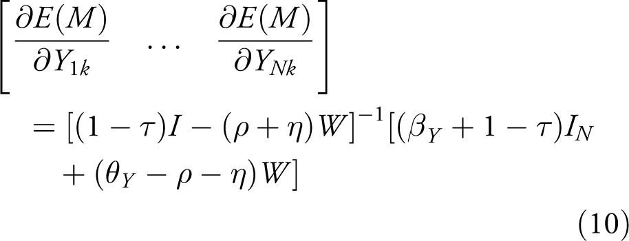
Departing from this partial derivative interpretation, we also can identify the impact of a change in the level of GDP observed in a particular country on the military expenditure level of other countries, replacing it with

[\begin{matrix} \frac{\partial E (M)}{\partial Y_{1 k}} & \dots & \frac{\partial E (M)}{\partial Y_{N k}} \end{matrix}] = {[(1 - τ) I - (ρ + η) W]}^{- 1} [(β_{Y} + 1 - τ) I_{N} + (θ_{Y} - ρ - η) W]

Table I.

Spatial econometric models with different combinations of spatial lags and flexibility for country spillover effects

Model	Spatial lag(s)	Restriction(s)	Flexibility and country spillovers
SAR, Spatial autoregressive model*	WY	θ=0, λ=0	Constant ratios, global
SEM, Spatial error model	Wu	θ=0, ρ=0	Zero by construction
SLX, Spatial lag of X model	WX	ρ=λ=0	Fully flexible, local
SAC, Spatial autoregressive combined model**	WY, Wu	θ=0	Constant ratios, global
SDM, Spatial Durbin model	WY, WX	λ=0	Fully flexible, global
SDEM, Spatial Durbin error model	WX, Wu	ρ=0	Fully flexible, local

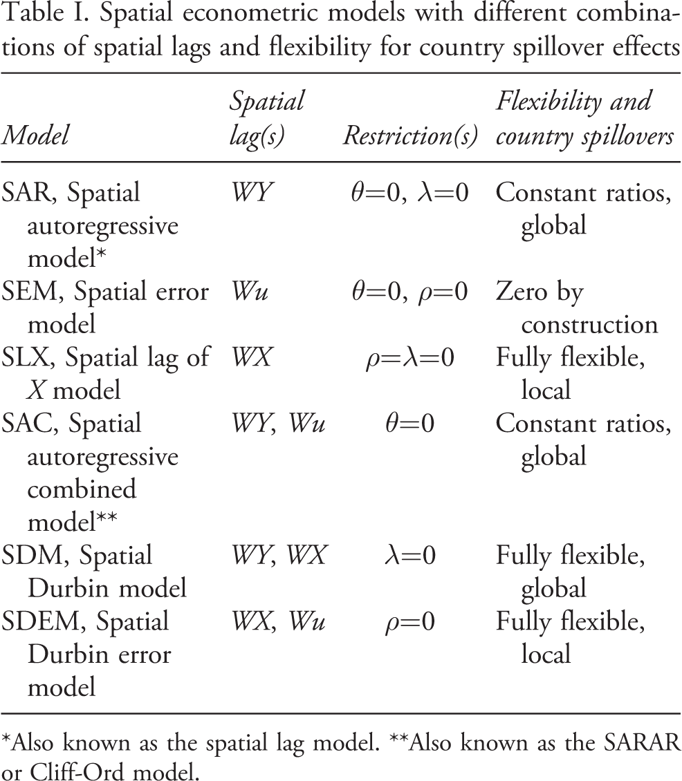
*Also known as the spatial lag model. **Also known as the SARAR or Cliff-Ord model.

The preceding discussion assumes that all spatial lags are included. In Table I we provide an overview of some simpler and more commonly used models in spatial econometrics literature, including their ability to calculate country spillovers. In particular, a limitation of SEM is that it imposes restrictions on the parameters (θ = 0, ρ = 0), so the off-diagonal elements of the matrix expression on the right-hand side of Equation (9) – that is, the country spillover effects – are reduced to 0. Accordingly, SEM cannot effectively measure the effects of spillovers (see also Beck, Gleditsch & Beardsley, 2006). For the SAR and SAC models, a proportionality relationship arises between the direct and spillover effects; if the ratio of spillover to direct effects for variable k equals a certain number, it equals this number for any other variable (Elhorst, 2010). From an empirical perspective, this link is unlikely. Therefore, only in models that include exogenous spatial lags (SLX, spatial Durbin model [SDM], spatial Durbin error model [SDEM]) can the spillover effects take different values across variables, in relation to their corresponding direct effects. Reinforcing the economic-theoretical derivation of the military expenditure demand function in Equation (5), this rationale provides a second reason to consider exogenous spatial lags observed in neighboring countries.

Finally, country spillover effects could be local or global. Local spillovers occur when ρ = 0 and θ ≠ 0, and countries are connected. If two countries i and j are unconnected, such that w_ij = 0, a change in x_ik of country i cannot affect the dependent variable of country j, and vice versa. Global spillovers instead occur when ρ ≠ 0 and θ = 0, regardless of whether countries are connected, so a change to x_ik of country i due to the spatial multiplier matrix (I–ρW)⁻¹ gets transmitted to all other countries, even if w_ij = 0. If military conflicts or the tension between countries at a local level can spread to other countries across the continent or around the world, even if they are not directly involved in the conflict, then the SDM or SAR specifications make more sense, due to their ability to capture such global spillovers. If other countries do not get involved though, the SDEM specification may be more appropriate, in that it captures only local country spillovers. The choice between local and global spillovers also relates to the specification of W. A sparse spatial weight matrix with only a limited number of non-zero elements, such as a binary contiguity matrix, is more likely to occur in combination with a global spillover model (ρ ≠ 0), whereas a dense spatial weight matrix in which many off-diagonal elements are non-zero (e.g. inverse distance matrix) is more likely in combination with a local spillover model (ρ = 0, θ ≠ 0). The choice of model and spatial weight matrix thus might be improved if they take place within a common framework.

Data, variables, and spatial weight matrices

The sample consists of 144 countries (see the Online appendix), over the period 1993–2007, for which we gathered data on the defense burden indicator from several sources: the WB, SIPRI, and the COW project. We also check the sensitivity of the results to the datasets. Spatial econometric research requires that the spatial panel be balanced; missing observations should be avoided as far as possible. This is because most software available for estimating spatial panels (Matlab, R, Stata) is written for complete datasets. Unfortunately, our datasets have missing observations: 1.5% of them in the COW and 7.1% in the WB/SIPRI dataset. By implementing trends from one dataset to the other, though, we construct a complete set of 2,160 observations (N = 144, T = 15), thereby assuming that the development of military expenditures over time in both datasets are comparable with each other. Due to this we were able to enlarge the sample from 120 to 144 countries. Yet for various reasons, some countries still are missing.³ Countries with adjacent neighbors that are not in the sample are indicated in the Online appendix; we detail how we dealt with this issue subsequently. Nevertheless, the sample is appropriate in that it contains multiple countries that frequently are engaged in tensions, such as Cuba, Israel, Lebanon, Iran, Syrian, Kuwait, Vietnam, Mali, Ethiopia, both Congos, and Colombia. We also collected data from multiple continents (Europe, Asia, Africa, North and South America, and Australia), so we can investigate whether the strength of the direct and country spillover effects differ across continents.

Similar to previous studies, we consider three categories of explanatory variables: economic, political, and strategic. The economic factors are GDP and population. The (log of the level of) GDP variable follows from the derived military demand function in Equation (5). We converted the GDP data into US 2005 dollars. In addition, we can measure the size of a country by its population, in line with prior literature that highlights the benefits of such a measure, including scale effects (Dunne & Perlo-Freeman, 2003a,b; Groot & van den Berg, 2009), security (Collier & Hoeffler, 2002), and public good effects (Fordham & Walker, 2005). However, the correlation coefficient between these two variables is high (approximately 0.63), so we decided to exclude this variable.⁴ Instead, if a country in the sample is adjacent to a country that is not part of the sample (see footnote 3), we control for the (log of the) population size of the non-sampled country relative to that of the sampled country. Countries that have not been sampled often represent serious threats to their neighbors, especially if they are relatively large. Therefore, this alternative variable might shed new light on the potential threat. The population data came from the Penn World Tables.⁵

For the political factors, we use the political regime of a country, which often functions as a determinant of military expenditures. Maizels & Nissanke (1986) suggest that the nature of the state is an important determinant; a military dictatorship likely maintains a larger military establishment than a democracy. Many studies adopt similar reasoning (e.g. Collier & Hoeffler, 2007; Goldsmith, 2007; Groot & van den Berg, 2009; Mulligan, Gil & Sala-i-Martin, 2004). Fordham & Walker (2005) provide a more thorough reasoning, based on international relations theory and Kantian liberalism, arguing that liberal states allocate fewer resources to their militaries than autocratic states. Furthermore, domestic political pressures can lead to these differences. Higher military expenditures during peacetime may adversely affect the nation as a whole, because resources allocated to military purposes come at the expense of support for highly valued social goods, such as education. Such military spending also might threaten civil liberties and political freedom – values with high standing in democratic countries. Therefore, most people in democratic countries likely oppose high military spending. In contrast, in autocratic states, small groups of people benefit from preparations for war, if they have the power to influence or control military decisions, and the military can function in a suppressive role, eliminating potential competitors of a dictator (Groot & van den Berg, 2009). It is thus in the best interest of the dictator to support the military and allocate substantial resources to military budgets. We accordingly expect a positive relationship between military expenditures and more autocratic regimes, but a negative relationship with democratic regimes. To describe the political regime of each country, we use the Polity2 variable from the Polity IV project dataset (Marshall, 2014). This indicator ranges from –10 to +10, where –10 indicates strongly autocratic and +10 is strongly democratic.

Finally, strategic factors involving relations between two or more countries may affect military spending. Previous studies indicate a significant relationship of international wars (e.g. Collier & Hoeffler, 2002, 2007; Dunne & Perlo-Freeman, 2003a,b; Goldsmith, 2007) and also suggest the impact of the closely related variable of civil war. According to Collier & Hoeffler (2002), civil wars are now many times more common than interstate wars, and the risk of rebellion may be more influential on levels of military expenditure than is the threat of an international war. The effects of internal and external wars might differ (Fordham & Walker, 2005), so we distinguish them. Specifically, we extracted data from the Major Episodes of Political Violence dataset, as provided by the Center of Systemic Peace. For the occurrence of international wars, we use the Inttot variable, which sums the magnitude scores for international violence and warfare. For civil wars, the Civtot variable is composed of both civil and ethnic violence and warfare. The scores for both types range from 0 (no war) to 10 (greatest), defined by the systematic and sustained use of lethal violence by organized groups that result in at least 500 directly related deaths over the course of an episode of war (Marshall, 2010).

For this study, we use three principles to construct eight spatial weight principles:

Sharing a common land or maritime border (Goldsmith, 2007; Skogstad, 2016) implies the first-order binary contiguity matrix, W1. Maritime borders are based on the United Nations Convention on the Law of the Sea and additional sources further explaining this convention.

The influence of a country might go beyond its immediate neighbors, as implied by the inverse distance matrix by Goldsmith (2007) and the different cut-off points by Quiroz Florez (2011). Therefore, we also consider a second-order binary contiguity matrix, W2.

A country may respond to the threat of even more distant countries, which is also the main reason that elements of the weight matrix within a certain radius of a country are not always set to 0. We accordingly include a third-order binary contiguity matrix, W3.

Quiroz Florez (2011) considers spatial weight matrices based on alliances, which also might be covered by the spatial autoregressive parameter ρ in Equation (1), corresponding to one of the factors in Goldsmith’s (2006) model that cause countries to maintain minimal defensive forces. As an alternative, we can construct a so-called Enemy matrix, according to countries that are each other’s sworn enemies, using data from the Uppsala Conflict Data Program.

A large overlap arises between Enemy and W1, so we combine these matrices, such that w_ij is set to equal 1 if the corresponding element in one of these two underlying matrices also equals 1. This matrix accordingly is denoted W1 + Enemy.

Skogstad (2016) notes countries’ ability to project their military power worldwide. The five superpowers in the world, the United States, Russia, China, United Kingdom, and France, also are the permanent members of the UN Security Council. Therefore, we construct a matrix in which all five countries interact, then combine it with the first-order binary contiguity matrix to form W1 + Superpowers.

The dominance of the United Kingdom and France largely stems from their historical and continuing role as colonizers of overseas territories. To distinguish each main country from its overseas territories, we base our contiguity matrices on immediate neighbors of the United Kingdom and France within Europe. Another way instead to model dominance is to assume that the five superpowers react to foreign threats everywhere, regardless of the country involved. To operationalize this potential relationship, we assume each country part of the dataset is a ‘neighbor’ of these five dominant countries, but not vice versa. Combined with the first-order binary contiguity matrix, this approach produces the matrix W1 + Dominance.⁶

An overall matrix combines the principles of first-order binary contiguity, enemy, and superpowers: W1 + Enemy + Superpowers.

Finally, all the matrices are row normalized, which is standard in spatial econometrics literature when the elements of W have a binary (0/1) character.

Results

Table II contains the Bayesian posterior model probabilities of the different models (SAR, SDM, SEM, SDEM), in combination with the eight proposed spatial weight matrices. We calculated these probabilities for both static and dynamic versions of the model specifications; the latter also contain the defense burden indicator lagged in time, space, and both space and time (Equations (6a) versus (1a)). With these probabilities we can simultaneously identify the most likely spatial econometric model and the most likely spatial weight matrix. The probabilities are based on the log-marginal likelihood obtained by integrating out all parameters of the model over the entire parameter space on which they are defined. In addition, they are normalized such that the probabilities of all 32 combinations sum to 1. This normalization is based on the (non-linear) property that the Bayesian posterior model probability increases if the log-marginal

Table II.

Simultaneous Bayesian comparison of model specifications and spatial weight matrices

Data	Model	W1	W2	W3	Enemy	W1 + Enemy	W1 + Superpowers	W1 + Dominance	W1 + Enemy + Superpowers	Row total
COW Static model	SAR	0.1449	0.0000	0.0000	0.0000	0.0224	0.1435	0.2838	0.0244	0.6190
	SDM	0.0054	0.0000	0.0000	0.0000	0.0026	0.0052	0.0119	0.0028	0.0279
	SEM	0.0625	0.0000	0.0000	0.0000	0.0098	0.0676	0.1603	0.0111	0.3113
	SDEM	0.0074	0.0000	0.0000	0.0000	0.0033	0.0073	0.0202	0.0036	0.0418
COW Dynamic model	SAR	0.2335	0.0000	0.0000	0.0000	0.0315	0.2547	0.4171	0.0350	0.9719
	SDM	0.0002	0.0000	0.0000	0.0000	0.0000	0.0002	0.0004	0.0000	0.0009
	SEM	0.0043	0.0000	0.0000	0.0000	0.0016	0.0056	0.0118	0.0018	0.0252
	SDEM	0.0004	0.0000	0.0000	0.0000	0.0001	0.0004	0.0010	0.0001	0.0020
WB/SIPRI Static model	SAR	0.0016	0.0061	0.5162	0.0020	0.0019	0.0015	0.0016	0.0019	0.5328
	SDM	0.0081	0.0004	0.0520	0.0294	0.0055	0.0072	0.0081	0.0047	0.1155
	SEM	0.0013	0.0044	0.2510	0.0040	0.0013	0.0013	0.0013	0.0013	0.2660
	SDEM	0.0084	0.0003	0.0235	0.0275	0.0053	0.0076	0.0086	0.0086	0.0857
WB/SIPRI Dynamic model	SAR	0.0382	0.0645	0.2365	0.0353	0.0390	0.0383	0.0381	0.0390	0.5288
	SDM	0.0001	0.0002	0.0259	0.0287	0.0001	0.0001	0.0001	0.0001	0.0551
	SEM	0.0411	0.0480	0.0835	0.0387	0.0382	0.0413	0.0411	0.0382	0.3701
	SDEM	0.0001	0.0002	0.0181	0.0272	0.0001	0.0001	0.0001	0.0001	0.0459

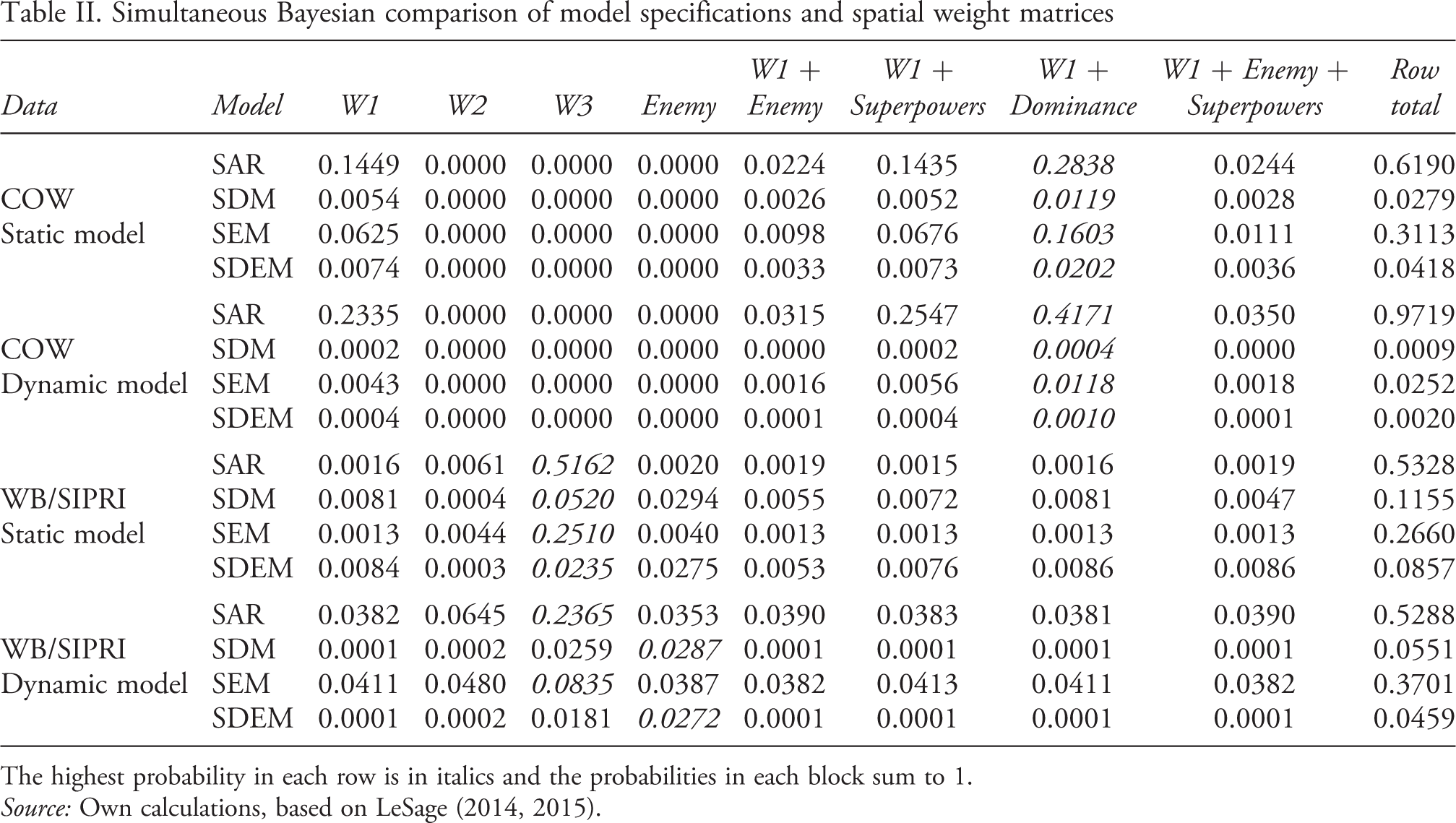
The highest probability in each row is in italics and the probabilities in each block sum to 1.

Source: Own calculations, based on LeSage (2014, 2015).

likelihood value of one model or one W exceeds that of another model or W. Full details can be found in LeSage (2014); the Matlab code used to carry out these comparisons is available in LeSage (2015).

The results in Table II show that the SAR model outperforms the other models in almost all 32 cases, for both the WB/SIPRI and COW datasets. Row totals for this model range from 0.5288 based on the first, to 0.9717 for the second dataset. This result is striking, especially considering that the SAR model is much simpler than the SDM specification and requires that the coefficients of all exogenous spatial lags are jointly insignificant (θ = 0). This finding corroborates previous approaches by Goldsmith (2007), Quiroz Flores (2011), and Skogstad (2016). The spatial interaction among countries appears driven only by the endogenous spatial lag, and countries adapt their defense burden ratio (or military expenditures) to those of their neighbors but not to other variables observed in neighboring countries. Thus the extension of the security function with the WX variable in Equation (4) seems unnecessary.

The most likely spatial weight matrix differs across the two datasets. The COW dataset favors the first-order binary contiguity matrix, whose performance improves when combined with the dominant position of the five superpowers and the proposition that they react to military activities all over the world. This matrix outperforms others no matter which spatial econometric model is used. The WB/SIPRI dataset instead favors the third-order binary contiguity matrix, in line with Quiroz Florez (2011), who also uses WB data and sets the elements of the weight matrix equal to 0 only outside a certain radius of a country. However, since the SAR model produces global country spillover effects, it is more likely to occur in combination with a sparse spatial weight matrix. In view of this, we determined the average number of neighbors of each country in the sample based on these two W matrices. It equals 9.3 for the W1 + Dominance matrix and 35.5 for the W3 matrix; in both cases the average number of adjacent neighbors based solely on land or maritime borders is 4.7. Departing from the principle of sparsity, the W1 + Dominance matrix thus seems to offer a better choice than the W3 matrix.

In Table III we report the estimation results of the dynamic SAR specification, based on the COW dataset and the W1 + Dominance matrix. The model parameters were estimated using the bias-corrected maximum likelihood estimator developed by Lee & Yu (2010).⁷ The results confirm some of the results of previous studies. For

Table III.

Results of the dynamic SAR model, with defense burden ratio as the dependent variable, COW data, and W = W1 + Dominance

Determinants	Coefficients	Short-term effects		Long-term effects		Short-term effects SDM		Short-term effects SAR military expenditures
Determinants	Coefficients	Direct	Spillover	Direct	Spillover	Direct	Spillover	Direct	Spillover
W*Ln(M/GDP) _t (ρ)	0.633*** (25.38)
Ln(M/GDP) _t (τ)	0.244*** (7.44)
Ln(M/GDP) _t _–1 (η)	–0.061 (–0.95)
Ln(GDP) (β_Y )	–0.284*** (–3.89)	–0.285** (–3.22)	–0.088** (–2.76)	–0.823** (–3.20)	–0.798^† (–1.73)	–0.285** (–3.07)	–0.089 (–0.46)
Ln(Population non-sampled/Population sampled country) (β)	0.538* (1.95)	0.552 (1.57)	0.169 (1.53)	1.594 (1.57)	1.535 (1.24)	0.527 (1.48)	0.509 (0.69)	0.359 (1.14)	0.136 (1.13)
International war (β)	0.067* (1.88)	0.069^† (1.76)	0.021^† (1.65)	0.200^† (1.74)	0.192 (1.31)	0.062 (1.52)	–0.032 (–0.35)	0.061^† (1.75)	0.023^† (1.69)
Civil war (β)	0.009 (0.71)	0.008 (0.61)	0.003 (0.59)	0.024 (0.60)	0.024 (0.53)	0.011 (0.76)	0.029 (0.84)	0.002 (0.12)	0.001 (0.12)
Political regime (β)	–0.008** (–2.25)	–0.009^† (–1.77)	–0.003^† (–1.71)	–0.024^† (–1.77)	–0.023 (–1.36)	–0.009^† (–1.80)	–0.016 (–1.43)	–0.008* (–1.97)	–0.003^† (–1.86)
Effect of GDP on M		0.727** (8.22)	0.244** (4.87)	0.246 (0.96)	0.236 (0.85)	0.715** (7.70)	–0.090 (0.46)	0.102 (1.33)	–0.159 (–0.90)
Observations	2,016					2,016
R²	0.779					0.800
Log-likelihood	–925.9					–924.1

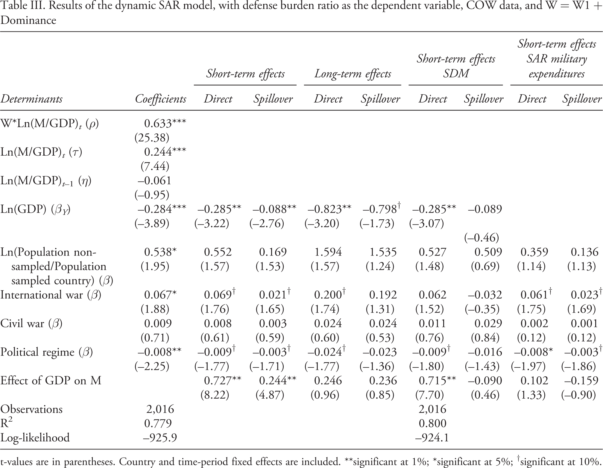
t-values are in parentheses. Country and time-period fixed effects are included. **significant at 1%; *significant at 5%; ^†significant at 10%.

example, the defense burden indicator strongly depends on its value in the previous year, or internal habit persistence; its coefficient amounts to 0.633 and is highly significant (1% level). We find no evidence of what Korniotis (2010) labels external habit persistence; the coefficient of the defense burden observed in neighboring countries in the previous period is negative but insignificant (–0.061, t-value = –0.95). However, countries respond to the defense burden set in neighboring countries in the same year, such that the coefficient ρ takes a positive value of 0.244 and is highly significant (t-value = 7.44), in line with the common feature of horizontal interaction among countries (Brueckner, 2003). The inclusion of the endogenous spatial lag has a downward effect on the internal habit persistence parameter, which helps explain why studies that do not control for an endogenous spatial lag tend to find slightly higher values for the persistence parameter (e.g. DiGiuseppe [2015] versus Goldsmith [2007]). A necessary and sufficient condition for stationarity, τ + ρ + η = 0.633 + 0.244 − 0.061 = 0.816 < 1, also is satisfied. To investigate the (null) hypothesis whether country fixed effects may be replaced by a common intercept and thus are jointly insignificant, we performed a likelihood ratio (LR) test. The results (349.6, with 143 degrees of freedom [df], p < 0.01) indicate that this hypothesis must be rejected. Similarly, the hypothesis that the time-period fixed effects are jointly insignificant must be rejected (34.2, 13 df, p < 0.01). Therefore, we included these factors in all regressions. This finding also implies that the parameter estimates in previous studies that do not control for fixed effects, because they employ cross-sectional data, might be biased.

The coefficient estimates and short-term direct effects estimates derived from the parameter estimates using Equation (9) exhibit a plausible model structure. The direct effect of the GDP variable on the defense burden indicator is negative and significant but greater than –1; military expenditures increase with the level of GDP but less than proportionally. This result follows from the direct effect of GDP on the military expenditure (M) itself, as calculated using Equation (10). Non-sampled countries are experienced as threats to their neighbors, but the coefficient of this variable is not significant. The impact of an international war on a country’s military expenditure is positive and weakly significant, as well as greater in magnitude than that of civil wars (cf. Fordham & Walker, 2005). The direct effect of the political regime variable, –0.009, is small but weakly significant, implying that the defense burden indicator decreases with a higher level of democracy but increases with a higher level of autocracy (lower value on the –10 to +10 scale). This finding is in line with our expectation that relatively more autocratic regimes undertake higher military expenditures, and more democratic countries have relatively lower military expenditures. The five explanatory variables exhibit similar significance levels for the long-term direct effects, but their magnitudes almost triple.

Three of the five country spillover effects appear to be (weakly) significant in the short term, and one in the long term. It concerns the impact of GDP, political regime, and international wars. Military expenditures do not only increase with the level of GDP in the own country, but to a lesser extent also with that in neighboring countries. Countries also tend to spend more if they are adjacent to autocratic states or if neighboring states are involved in an international war. Conversely, they tend to spend less if they are adjacent to democratic states. These spillover effects are approximately one-third of the corresponding direct effects. This one-third is due to the proportionality relationship between the direct and spillover effects imposed by the SAR model. If we do not impose the restriction that the coefficients of all exogenous spatial lags are zero (θ ≠ 0) by estimating the dynamic SDM specification, which allows the country spillover effects to have the flexibility to take any value, they all lose their significance (see the column ‘Short-term effects SDM’ of Table III). However, in line with the Bayesian results in Table II, this model extension is no improvement over the dynamic SAR model: the hypothesis about whether it can be simplified to the dynamic SAR model, H₀: θ = 0, cannot be rejected (3.6, 6 df, p = 0.45). This implies that the empirical evidence in favor of the three significant country spillover effects in the short term hinges strongly on the previous finding that the spatial interaction among countries is driven only by the endogenous spatial lag.

The insignificant country spillover effects in the dynamic SDM also might reflect the focus on the defense burden, the data being used, or the restriction that the parameters are homogeneous across countries located on different continents. We report and discuss the results of three robustness checks, thereby focusing on short-term direct and country spillover effects. First, the defense burden indicator is replaced by military expenditures as the dependent variable, while the coefficients of ln(Y_t) and Wln(Y_t−1) are set to zero. The explanation behind this robustness check was set out below Equation (7), and the results are reported in the last column of Table III. As expected, the direct and country spillover effects are hardly affected by this. We find short-term effects that are similar in magnitude and significance levels. Only the short-term effects of GDP become much smaller. The reason is that the coefficients of ln(Y_t) and Wln(Y_t−1), when estimated, appear anything but zero and insignificant. Consequently, this zero restriction needs to be rejected.

The second check re-estimates the dynamic SAR specification with the WB/SIPRI dataset and replaces the spatial weight matrix by the third-order binary contiguity matrix, in line with the results in Table II. The first column of Table IV shows that the direct effects of the GDP and the political regime variables decrease in magnitude, and become less significant or even insignificant. Conversely, the direct effect of civil wars increases in magnitude and, just as the direct effect of international wars, becomes significant. The biggest change occurs in the country spillover effects. None of them is significant any more. According to this dataset, countries adapt their defense burden to that of their neighbors, but this has no effect on the country spillovers caused by the explanatory variables.

With our third robustness check, we note that such differences in emphasis also occur when researchers carry out separate analyses for countries located in Europe, Asia, America, and Asia (Gleditsch, 2002; Goldsmith, 2006, 2007; Quiroz Flores, 2011), in these cases based on the COW dataset.⁸ Since the choice of model and of W need to be made simultaneously, we repeated the Bayesian comparison approach and selected the most likely spatial econometric model and the most likely spatial weight matrix for each continent. The results differ per continent and are reported in Columns 2–5 of Table III. The direct effect of non-sampled countries, which was insignificant up to now, especially shows up in Europe. These countries were part of the former Yugoslavia; in the aftermath of that war, at the beginning of our observation period, they were still reporting very

Table IV.

Robustness checks for short-term direct and spillover effects

	(1) WB/SIPRI data		(2) Europe		(3) Asia		(4) America		(5) Africa
Determinants	Direct	Spillover	Direct	Spillover	Direct	Spillover	Direct	Spillover	Direct	Spillover
Ln(GDP)	–0.117^† (–1.76)	–0.002 (–0.10)	–0.298^† (–1.65)	–1.743* (–2.57)	–0.297 (–1.50)	–0.067 (–1.24)	0.532 (1.05)	2.273* (2.29)	–0.232^† (–1.91)	–0.248 (–0.24)
Ln(Population non-sampled/ Population sampled country)	0.192 (0.71)	0.002 (0.04)	1.862^† (1.84)	2.894 (0.80)	0.383 (0.54)	0.085 (0.49)	1.371 (1.28)	–0.198 (–0.08)	–0.288 (–0.50)	–0.432 (–0.14)
International war	0.070* (2.36)	0.001 (0.11)	0.088^† (1.71)	0.066 (0.34)	–0.045 (–0.50)	–0.010 (–0.45)	–0.162 (–0.51)	–0.362 (–0.81)	0.136** (3.47)	0.445^† (1.81)
Civil war	0.028* (2.53)	0.001 (0.13)			–0.006 (–0.18)	–0.001 (–0.18)	0.073 (1.10)	0.317* (2.05)	0.003 (0.18)	–0.080 (–0.61)
Political regime	–0.004 (–1.14)	–0.001 (0.13)	–0.006 (–0.64)	–0.010 (–0.23)	–0.003 (–0.33)	–0.001 (–0.29)	–0.015 (–0.43)	0.137* (2.26)	–0.011^† (–1.72)	–0.010 (–0.27)
Effect of GDP on M	0.883** (13.21)	0.013 (0.12)	0.702** (3.82)	–1.743* (–2.57)	0.713** (3.60)	0.161* (2.13)	1.532** (3.01)	2.273** (2.29)	0.768** (6.33)	–0.248 (–0.23)
Observations	2,016		476		616		280		616
R²	0.846		0.841		0.759		0.616		0.81

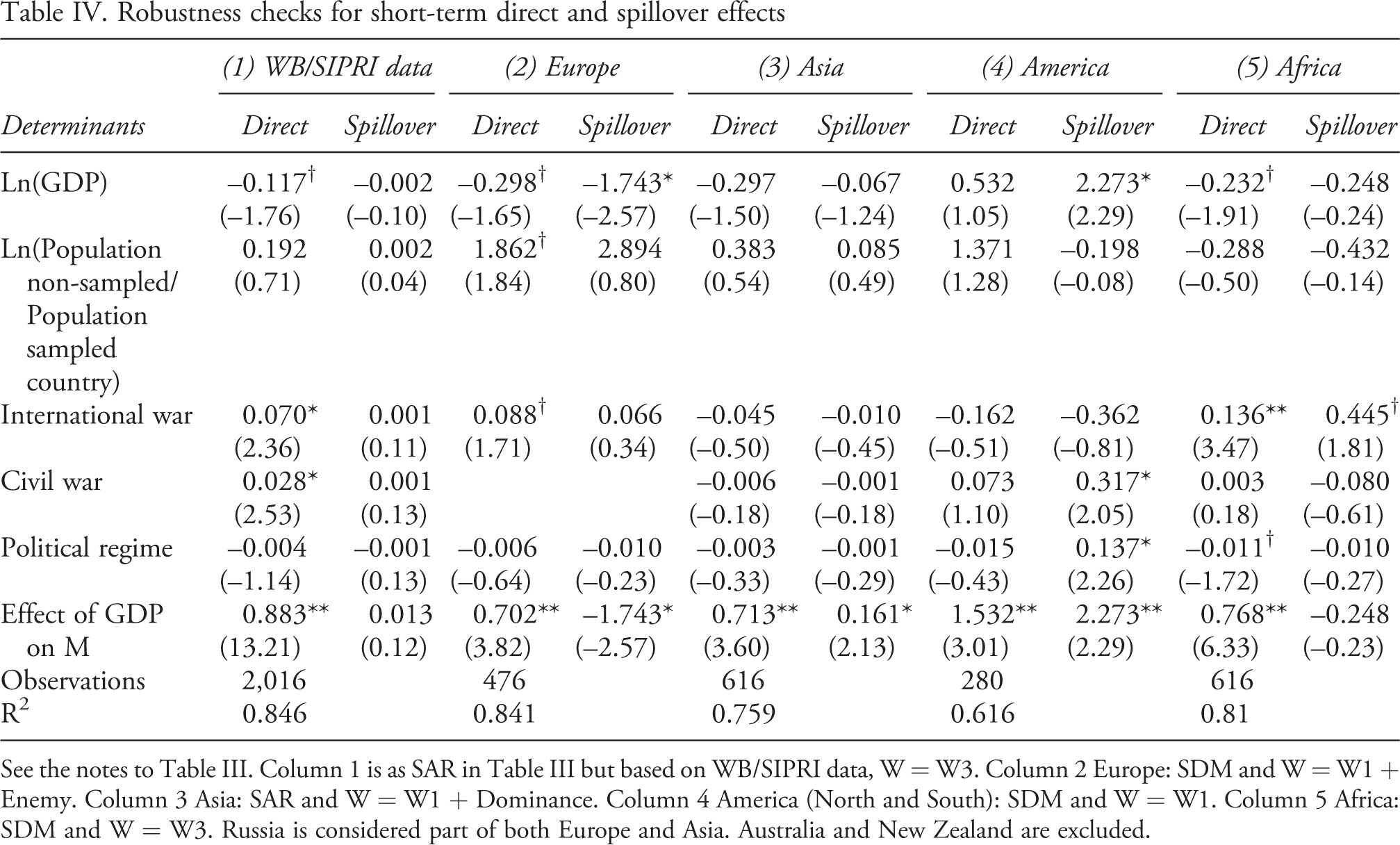
See the notes to Table III. Column 1 is as SAR in Table III but based on WB/SIPRI data, W = W3. Column 2 Europe: SDM and W = W1 + Enemy. Column 3 Asia: SAR and W = W1 + Dominance. Column 4 America (North and South): SDM and W = W1. Column 5 Africa: SDM and W = W3. Russia is considered part of both Europe and Asia. Australia and New Zealand are excluded.

high military expenditure levels, probably to protect themselves against countries surrounding them that were not part of the sample. The direct and country spillover effects of the GDP of countries located in the Americas are the only ones that appear significantly greater than 1. Apparently, American countries adapt their military expenditures more than proportionally to their own level of GDP and that of their neighbors, which is understandable considering that the average defense burden indicator on this continent is the lowest of all other continents during our sample period. However, in Europe, this country spillover effect is instead negative and significant. Apparently, European countries not only adapt their military expenditures less than proportionally to their level of GDP, but they even reduce it if their neighbors’ GDPs grow. As Sandler & Hartley (2001) argue, many European countries are members of an alliance (NATO), so they might not make additional investments in defense or reduce their defense expenditures to free-ride on their alliance partners. American countries are strongly affected by civil wars in neighboring countries (Mexico, Colombia, and Peru [until 1997]), in line with Phillips’s (2014) finding for developing countries. American countries are also weakly significantly affected by the political regimes of their neighbors. Like-minded countries on this continent, either autocratic or democratic, tend to push up each other’s military spending, similar to the result found for the GDP spillover effects. Finally, African countries are strongly affected by neighboring countries involved in an international war. In summary, when we conduct the analysis again, splitting the data across different continents, some or other country spillover effects become significant.

Conclusions

With this article, we have sought to gain better understanding of the impact of neighboring countries on military expenditures. The endogenous spatial lag appears to be the main driving force of spatial interaction effects; its coefficient takes a positive and significant value of 0.244. This positive value is in line with a common feature of horizontal interactions among governments (Brueckner, 2003) and with the SAR model applied in several previous studies (Goldsmith, 2007; Quiroz Flores, 2011; Skogstad, 2016). The evidence in favor of the SAR model is based on our application of a Bayesian comparison approach to four potential models (SAR, SEM, SDM, and SDEM), a method developed only recently.

The SAR model produces global spillover effects – that is, countries adapt their defense burden indicator or military expenditures to those of other countries, even if they are not neighbors – so the spatial weight matrix is likely to be sparse. The first-order binary contiguity matrix based on land or maritime borders, extended to include both the dominant position of the five countries that are permanent members of the UN Security Council and the proposition that they react to military activities of all countries, in combination with COW data, comes closest to this property of sparseness.

In contrast with the endogenous spatial lag, it is hard to find strong empirical evidence in favor of country spillover effects. Three variables – GDP, international wars, and political regime – produce (weakly) significant spillover in the short term, but this finding hinges strongly on the previous finding that the spatial interaction among countries is driven mainly by the endogenous spatial lag. We also find empirical evidence in favor of country spillover effects of civil wars when we conduct a separate analysis for American countries. Similarly, we find evidence in favor of spillover effects of the relative population size of non-sampled countries among European countries, of the political regime among American countries, and international wars among African countries.

We encourage the use of spatial panels rather than cross-sectional data in further research, because these data offer means to control for habit persistence and for country and time fixed effects. Both of these types of controls appear highly significant.

Footnotes

Replication data

The Online appendix, the dataset, codebook, and m-files for the empirical analysis in this article can be found at .

Acknowledgements

The authors thank Ron Smith (Birkbeck College) and Özlem Önder (Ege University), three anonymous reviewers, and Michael Brzoska (JPR’s Associate Editor) for their useful comments; they also thank Arjan Huizinga and Nannette Stoffers (University of Groningen) for their cooperation on a previous version of this article.

Funding

This research was supported by the Scientific and Technological Research Council of Turkey under grant number 112K020, for which the authors are indebted.

Notes

References

Baltagi

Badi H

(2004) Econometric Analysis of Panel Data. Chichester: Wiley.

Beck

Nathaniel

Gleditsch

Kristian Skrede

Beardsley

Kyle

(2006) Space is more than geography: Using spatial econometrics in the study of political economy. International Studies Quarterly 50(1): 27–44.

Brueckner

Jan K

(2003) Strategic interaction among governments: An overview of empirical studies. International Regional Science Review 26(2): 175–188.

Collier

Paul

Hoeffler

Anke

(2002) Military expenditure: Threats, aid, and arms races. World Bank Policy Research Working Paper no. 2927 (http://documents.worldbank.org/curated/en/162611468739486410/Military-expenditure-threats-aid-and-arms-races).

Collier

Paul

Hoeffler

Anke

(2007) Unintended consequences: Does aid promote arms races? Oxford Bulletin of Economics and Statistics 69(1): 1–27.

Corrado

Luisa

Fingleton

Bernard

(2012) Where is the economics in spatial econometrics? Journal of Regional Science 52(2): 210–239.

DiGiuseppe

Matthew

(2015) Guns, butter, and debt: Sovereign creditworthiness and military expenditure. Journal of Peace Research 52(5): 680–693.

Dunne

J Paul

Perlo-Freeman

Sam

(2003a) The demand for military spending in developing countries. International Review of Applied Economics 17(1): 23–48.

Dunne

J Paul

Perlo-Freeman

Sam

(2003b) The demand for military spending in developing countries: A dynamic panel analysis. Defence and Peace Economics 14(6): 461–474.

10.

Elhorst

J Paul

(2010) Applied spatial econometrics: Raising the bar. Spatial Economic Analysis 5(1): 9–28.

11.

Elhorst

J Paul

(2014) Spatial Econometrics: From Cross-Sectional Data to Spatial Panels. Heidelberg: Springer.

12.

Firmino Costa da Silva

Diego

Elhorst

J Paul

Neto

Raul da Mota Silveira

(2017) Urban and rural population growth in a spatial panel of municipalities. Regional Studies 51(6): 894–908.

13.

Fordham

Benjamin O

Walker

Thomas C

(2005) Kantian liberalism, regime type, and military resource allocation: Do democracies spend less? International Studies Quarterly 49(1): 141–157.

14.

Gleditsch

Kristian Skrede

(2002) All International Politics is Local: The Diffusion of Conflict, Integration, and Democratization. Ann Arbor, MI: University of Michigan Press.

15.

Goldsmith

Benjamin E

(2006) A universal proposition? Region, conflict, war, and the robustness of the liberal peace. European Journal of International Relations 12(4): 533–563.

16.

Goldsmith

Benjamin E

(2007) Arms racing in ‘space’: Spatial modelling of military spending around the world. Australian Journal of Political Science 42(3): 419–440.

17.

Groot

Loek

Berg

Vincent van den

(2009) Inequality in military expenditures and the Samuelson rule. Defence and Peace Economics 20(1): 43–67.

18.

Halleck Vega

Solmaria

Elhorst

J Paul

(2015) The SLX model. Journal of Regional Science 55(3): 339–363.

19.

Korniotis

George M

(2010) Estimating panel models with internal and external habit formation. Journal of Business and Economic Statistics 28(1): 145–158.

20.

Lee

Lung-fei

Jihai

(2010) Some recent developments in spatial panel data models. Regional Science and Urban Economics 40(5): 255–271.

21.

LeSage

James P

(2014) Spatial econometric panel data model specification: A Bayesian approach. Spatial Statistics 9(August): 122–145.

22.

LeSage

James P

(2015) Software for Bayesian cross section and panel spatial model comparison. Journal of Geographical Systems 17(4): 297–310.

23.

LeSage

James P

Kelley Pace

(2009) Introduction to Spatial Econometrics. Baton Rouge, LA: CRC/Taylor & Francis.

24.

Maizels

Alfred

Nissanke

Machiko K

(1986) The determinants of military expenditures in developing countries. World Development 14(9): 1125–1140.

25.

Marshall

Monty G

(2010) Major episodes of political violence (MEPV) and conflict regions, 1946–2008 (www.systemicpeace.org/warlist/warlist.htm).

26.

Marshall

Monty G

(2014) Polity IV project: Political regime characteristics and transitions, 1800–2013 (www.systemicpeace.org/polity/polity4.htm).

27.

Mulligan

Casey B

Gil

Ricard

Sala-i-Martin

Xavier

(2004) Do democracies have different public policies than nondemocracies? Journal of Economic Perspectives 18(1): 51–74.

28.

Nordhaus

William

Oneal

John R

Russett

Bruce

(2012) The effects of the international security environment on national military expenditures: A multicountry study. International Organization 66(3): 491–513.

29.

Phillips

Brian J

(2014) Civil war, spillovers and neighbors’ military spending. Conflict Managmenent and Peace Science 32(4): 425–442.

30.

Quiroz Flores

Alejandro

(2011) Alliances as contiguity in spatial models of military expenditures. Conflict Management and Peace Science 28(4): 402–418.

31.

Richardson

Lewis F

(1960) Arms and Insecurity: A Mathematical Study of Causes and Origins of War. Pittsburgh, PA: Boxwood.

32.

Sandler

Todd

Hartley

Keith

(2001) Economics of alliances: The lessons for collective action. Journal of Economic Literature 39(3): 869–896.

33.

Skogstad

Karl

(2016) Defence budgets in the post-Cold War era: A spatial econometric approach. Defence and Peace Economics 27(3): 323–352.

34.

Smith

Ron P

(1989) Models of military demand expenditure. Journal of Applied Econometrics 4(4): 345–359.

35.

Smith

Ron P

(1995) The demand for military expenditure. In: Hartley

Keith

Sandler

Todd

(eds) Handbook of Defense Economics, Volume 1. Amsterdam: Elsevier Science, 69–87.

36.

Yildrim

Jülide

Öcal

Nadir

(2016) Miltary expenditure, economic growth and spatial spillovers. Defence and Peace Economics 27(1): 87–104.

Supplementary Material

Please find the following supplemental material available below.

For Open Access articles published under a Creative Commons License, all supplemental material carries the same license as the article it is associated with.

For non-Open Access articles published, all supplemental material carries a non-exclusive license, and permission requests for re-use of supplemental material or any part of supplemental material shall be sent directly to the copyright owner as specified in the copyright notice associated with the article.

0.00 MB

Impacts of neighboring countries on military expenditures

Abstract

Keywords

Introduction

Spatial lags and weights

Spatial model of military expenditures

Theory

Dynamics

Expenditures and defense burden

Spillovers

Data, variables, and spatial weight matrices

Results

Conclusions

Footnotes

Replication data

Acknowledgements

Funding

Notes

References

Supplementary Material