
Abstract
Contributions to the quantitative civil war literature increasingly rely on geo-referenced data and disaggregated research designs. While this is a welcome trend, it necessitates geographic information systems (GIS) skills and imposes new challenges for data collection and analysis. So far, solutions to these challenges differ between studies, obstructing direct comparison of findings and hampering replication and extension of earlier work. This article presents a standardized structure for storing, manipulating, and analyzing high-resolution spatial data. PRIO-GRID is a vector grid network with a resolution of 0.5 x 0.5 decimal degrees, covering all terrestrial areas of the world. Gridded data comprise inherently apolitical entities; the grid cells are fixed in time and space, they are insensitive to political boundaries and developments, and they are completely exogenous to likely features of interest, such as civil war outbreak, ethnic settlement patterns, extreme weather events, or the spatial distribution of wealth. Moreover, unlike other disaggregated approaches, gridded data may be scaled up or down in a consistent manner by varying the resolution of the grid. The released dataset comes with cell-specific information on a large selection of political, economic, demographic, environmental, and conflict variables for all years, 1946–2008. A simple descriptive data assessment of population density and economic activity is offered to demonstrate how PRIO-GRID may be applied in quantitative social science research.
Introduction
While the quantitative study of armed conflict traditionally is carried out at the country level, contemporary empirical work increasingly uses geographic information systems (GIS) data to capture conflict dynamics at a subnational level. Recent contributions to the disaggregation trend in cross-country research focus on conflict zones (e.g. Braithwaite, 2006; Buhaug & Gates, 2002), conflict events (e.g. O’Loughlin & Witmer, 2011; Raleigh et al., 2010), and conflict onset locations (e.g. Braithwaite, 2005; Buhaug, 2010). Likewise, the habitual unit of analysis – the country – is increasingly replaced by grid cells (e.g. Buhaug & Rød, 2006; Raleigh & Urdal, 2007), geographically distinct ethnic groups (e.g. Buhaug, Cederman & Rød, 2008; Weidmann, 2009) or subnational administrative entities (e.g. Murshed & Gates, 2005; Østby, Nordås & Rød, 2009) to better capture local variation. In addition, a host of local factors plausibly affecting the risk and course of armed conflict have become available in a geo-referenced format, such as population size/density (CIESIN, 2005), settlement areas of politically relevant ethnic groups (Wucherpfennig et al., 2011), economic activity (Nordhaus, 2006), natural resource sites (e.g. Lujala, Rød & Thieme, 2007), and various climate statistics (e.g. GPCC, 2010).
So far, there have been few attempts to coordinate these efforts. As a result, relevant datasets come in different formats, with different spatial resolutions, and rely on different data structures and coordinate systems (e.g. vector versus raster, point versus polygon data, NetCDF versus shapefiles, etc.). Many of these datasets are not easily combined and converted to a common unit of analysis. It currently takes in-depth GIS skills to be able to exploit the rich data and opportunities offered by disaggregated research designs. Most social science scholars do not possess such skills.
This article presents a solution to the technical challenges incurred by using GIS data. PRIO-GRID is a spatio-temporal grid structure constructed to aid the compilation, management, and analysis of spatial data within a time-consistent framework. It consists of quadratic grid cells that jointly cover all terrestrial areas of the world. The basic (static) version of PRIO-GRID contains cell-specific information on a limited selection of core variables (e.g. cell ID, cell area, population, and terrain characteristics), which may be joined with yearly files containing time-varying information measured specifically for each geographic cell (e.g. country code/name, population size, ethnic composition, etc.). Although PRIO-GRID was designed with peace and conflict research in mind, its potential applicability extends well beyond the study of civil war.
In the following, we briefly review arguments for when and how spatial disaggregation is pertinent and describe how this has been carried out in earlier research. The main content of the article is the presentation of PRIO-GRID – its structure, content, and applicability. We offer some examples to highlight how PRIO-GRID may be used to investigate new location-sensitive questions and offer more precise empirical tests of prevalent theories of civil war. We also discuss the prevalence of spatial autocorrelation in geographic data.
Disaggregation: Motives and solutions
What causes civil war? Why do some civil wars last longer than others? Such questions have been subject to systematic scientific scrutiny for decades. Until recently, however, quantitative comparable analyses have been carried out almost exclusively at the level of independent states. Consequently, India – with all its geographic, cultural, political, and socio-economic facets – is treated as a homogenous entity in exactly the same manner as, say, Iceland. This assumption of unit homogeneity may be trivial in some settings but is clearly problematic in others. For example, by modeling civil war outbreak as a function of gross domestic product (GDP) per capita, country population size, ethno-linguistic fractionalization, and other conventional country-level correlates of civil war, we may deduce that India is at higher risk of civil war than Iceland, but we are unable to understand why only some parts of India have a recent history of violence, much less get credible estimates of the local conflict risk. As Buhaug & Lujala (2005) show, there are often significant discrepancies between national aggregates and local-level conditions, and conflict zones are rarely representative of the country at large. Indeed, Cederman & Gleditsch (2009: 488) argue that ‘many of the non-findings and conundrums in the existing cross-national research on civil war … follow at least partly from the near exclusive reliance on country-level attributes.’
As a result of advances in technology and data availability, there has been a wave of disaggregated conflict studies in recent years, perhaps best epitomized by the special issue of the Journal of Conflict Resolution on ‘Disaggregating Civil War’ in 2009. We refer to the introduction (Cederman & Gleditsch, 2009) and subsequent articles in that issue for reviews of the earlier literature, and Sambanis (2004) for a critical discussion of limits to country-level research. At this stage, we limit ourselves to briefly presenting a few alternative means of disaggregation. 1
We can identify three broad departures from the conventional country-level analysis of armed conflict. First, a number of recent publications focus on subnational groups and actors. For example, the Minorities at Risk project (Gurr, 1993) has collected data on 283 targeted politically active minorities and provides information on organizational structure and violent behavior for some of these groups. Öberg’s (2002) study of ethnic rebellion introduced a link between ethnic groups and rebel organizations, analyzed against a control group of 370 ethnic groups without an armed agent (Öberg, 2002: 97). More recently, Wimmer, Cederman & Min (2009) have constructed a catalogue of politically relevant ethnic groups for most countries in the world and coded these groups against the conflicts in the UCDP/PRIO Armed Conflict dataset.
Cunningham, Gleditsch & Salehyan (2009) introduce a new dataset, largely based on data from UCDP, focusing on variables specific to conflict organizations, such as troop size, organizational aspects, and technology. The Non-State Actor dataset is limited to organizations involved in conflict. It does not feature any control group, hence the dataset cannot be used to assess why some groups are involved in conflict and other are not. A complementary approach is offered by Carey, Mitchell & Lowe (2009), who focus on conflict organizations that are associated with the government, so-called Pro-Government Armed Groups.
A second set of contributions uses subnational administrative entities as the unit of observation (e.g. Østby, Nordås & Rød, 2009; Weidmann & Ward, 2010). Districts and provinces are easily identifiable, with clear geographic boundaries, and their political relevance is undisputed. This approach is quite similar to dividing the world into countries, just at a different scale. However, the composition and outline of political subunits are prone to change over time and their extent and function may vary substantially between countries. While these issues have been known for country-level studies, the magnitude of the problem is much larger for the subnational level. A geo-referenced, global time-series dataset on subnational units that will remedy some of these challenges is currently under development at ETH Zurich (Deiwiks, 2010). While that project is very useful on its own merits, the underlying data structure is not ideal for managing non-political variables and conducting comparative cross-national research.
The final category of disaggregated civil war studies substitutes countries with grid cells that allow for within-country variation (e.g. Buhaug & Rød, 2006; Raleigh & Hegre, 2009). This approach is sometimes referred to as quadrat sampling in spatial analysis, where data are collected using an overlay of a regular form, such as squares or hexagonal polygons (de Smith, Goodchild & Longley, 2007). Gridded data are inherently apolitical entities; they are fixed in time as well as space and are insensitive to political boundaries and developments. For this reason, the grid structure might be deemed worthless and irrelevant for conflict research. Yet, the stationary nature of the grid structure is a significant advantage, allowing for units of observation that are identical in shape and completely exogenous to the feature of interest (e.g. outbreak or incidence of civil war). Moreover, unlike other disaggregated approaches, gridded data may be scaled up or down by varying the resolution of the grid. Hence, we find the grid structure ideal to our objective: to generate a unified spatial data structure that can facilitate GIS-based research on civil war (as well as other phenomena of interest).
Table I illustrates the diversity in disaggregated approaches to the quantitative study of civil war. In the next section, we present the structure and content of PRIO-GRID, before offering a simple illustration of how it can be applied in social science research.
Selected disaggregated studies of civil war
Why standardization?
The departure from the singular country-year data structure has been multifaceted. The plethora of methodological approaches to the local study of civil war opens up possibilities for empirical triangulation and solid generalizations. However, the many alternative solutions found are ineffective for the field as a whole. Data collected by one project are often incompatible with data from other projects. Time and money are wasted trying to reconcile basic but arbitrary differences. The standardization we propose is limited to the ways in which gridded data are collected, managed, and stored, but it is important nonetheless.
GIS data come in a variety of different formats. A central distinction runs between raster data (analogous to bitmap or image pixels) and vector data. The latter type is further divided into point, line, and polygon data. Each data format has comparable advantages and disadvantages, and converting data between formats (e.g. from raster to vector) is complicated and may result in loss of information. An additional challenge concerns the unit resolution, which may range from exact geographic coordinates of point features (e.g. oil rigs) via rasterized data at various pixel resolutions (e.g. oil fields) to data available at federal state level (e.g. value of oil production). Various resampling techniques include aggregation of higher-resolution data by calculating mean values for each desired unit of observation, disaggregation of same values into smaller units, and recalculation of cell values by applying geospatial interpolation techniques (see Longley et al., 2005).
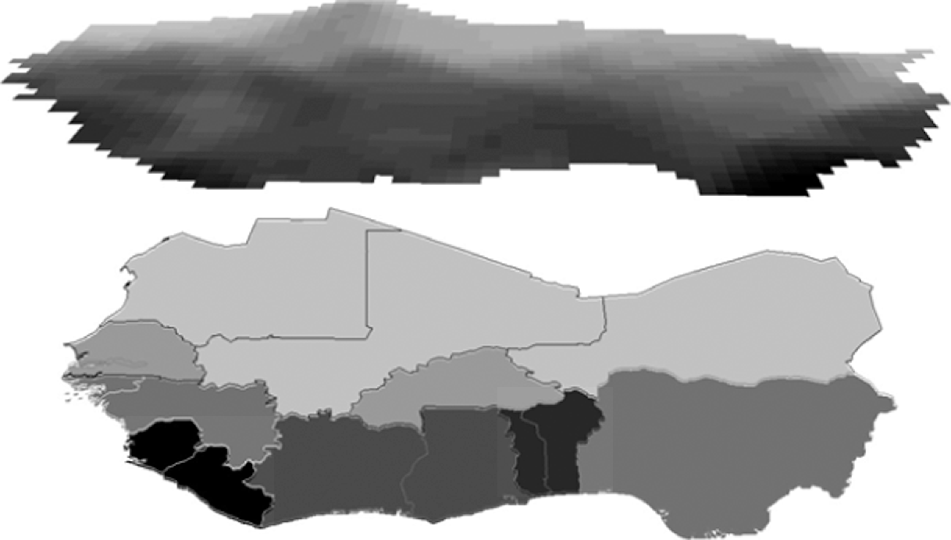
Figure 1 illustrates how high-resolution land class raster data are converted into a smaller set of observations in the vector-based grid system. Only trained GIS experts are able to combine such data and convert the variables to a common set of observations. By streamlining spatial data in a unified grid structure, we believe PRIO-GRID constitutes a useful point of departure for scholars working with spatial data.
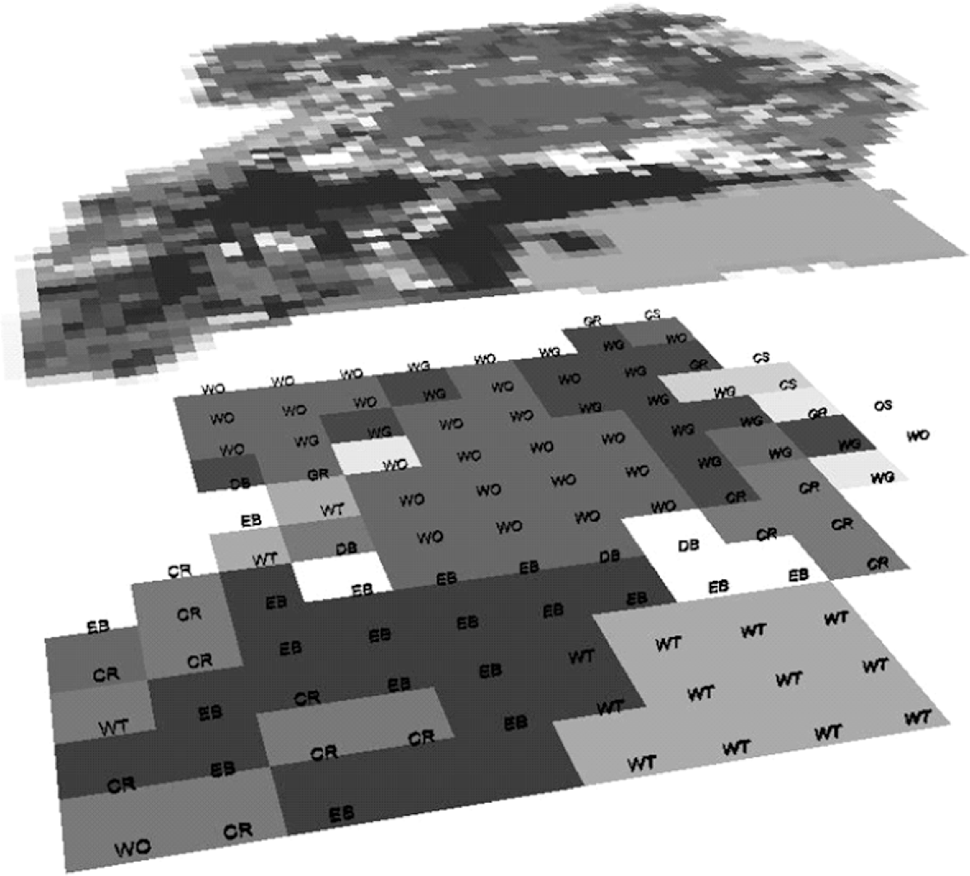
Conversions of a high-resolution land cover raster to grid structure
PRIO-GRID: Structure and content
PRIO-GRID is constructed by imposing a quadratic grid on the two-dimensional terrestrial plane using vector shapefiles, where each cell in the grid is represented by a square polygon vector feature. Each cell’s attributes are represented in the attached dBase (.dbf) attribute table, which includes the variables and values for each cell observation in the grid. 2 Spatially, the grid adheres to the dominant geographic coordinate system (the World Geodesic System, WGS84) where the arcs separating the grid cells are defined at exactly 0.5 decimal degree intervals latitude and longitude, originating from the southwestern corner of the coordinate grid (90°S, 180°W). The complete global grid matrix consists of 360 rows x 720 columns, amounting to 259,200 grid cells. A large majority of these cells carry little relevance in most applications as they cover oceans and other unpopulated areas, but 64,818 cells contain at least a tiny sliver of land (Antarctica excluded), that is, cell land area ≥ 0.01 km2 (slightly larger than a football pitch).
The chosen resolution is not coincidental: 0.5 decimal degrees latitude/longitude correspond to roughly 50 x 50 km at the equator. Hence, even very small countries such as Burundi or Bhutan are represented by multiple grid cells that allow within-country variation on spatial data. At the same time, the grid is sufficiently coarse to avoid excessively large data files (though nearly 65,000 observations in a single global cross-section hardly can be considered small). 3 The selected grid size also corresponds well with available GIS data on, for example, population size and other demographic components, infant mortality, and various climate statistics. Figure 2 gives a visualization of the spatial grid structure imposed on Southeast Asia.
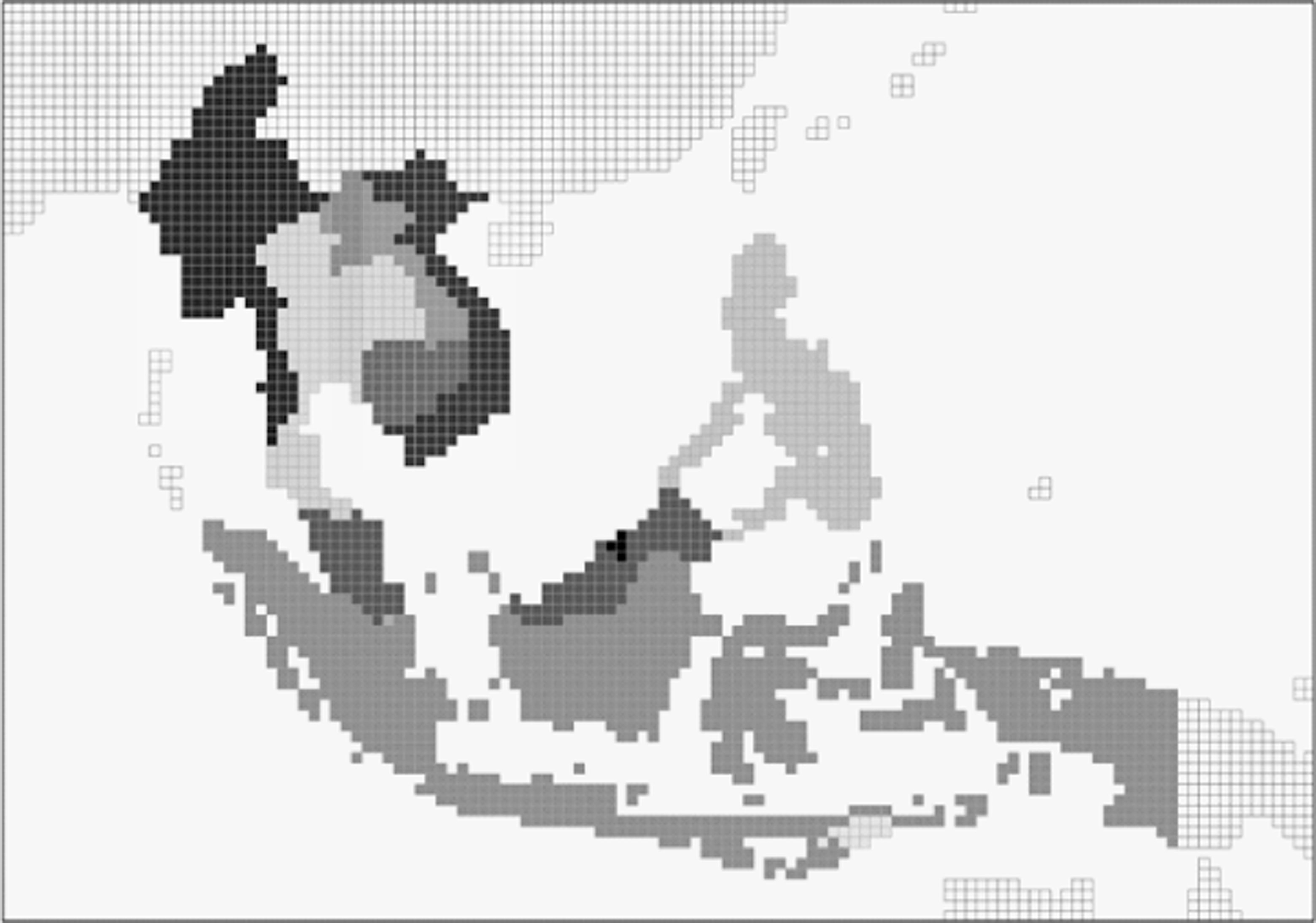
PRIO-GRID representation of Southeast Asia
PRIO-GRID consists of two sets of files. The first set is the static grid, which contains information on the outline and coordinate system of the grid, including a unique identifier for each cell (gid), stored in the attribute table. The static PRIO-GRID additionally contains a limited selection of time-invariant information. Among these are size of the landmass in each cell, expressed in square kilometers; cell-specific population size estimates, based on CIESIN’s (2005) Gridded Population of the World v. 3.0 dataset (four variables are provided, giving population estimates for 1990, 1995, 2000, and 2005, respectively); data on mountainous and closed forest terrain (expressed as percentage of cell area covered); estimates of the local level of economic activity, based on the G-Econ dataset (Nordhaus, 2006); and information on ethnic group settlements, represented by group ID variables for spatially distinct ethnic groups that are present in each cell, derived from the GeoEPR Dataset (Wucherpfennig et al., 2011). See the codebook (Tollefsen, 2012) for further details on the data included in PRIO-GRID.
The second set of files in PRIO-GRID contains time-varying indicators. 4 These files come in an annual format and are available for all years, 1946–2008. Each of the yearly grids presents a snapshot of the world for the corresponding year. A key component of the grid year files is the inclusion of country information, which allows combining measures of local conditions and events with country-level information (e.g. democracy score). Since the PRIO-GRID structure in effect is a two-dimensional spatial matrix, it contains no overlapping cells. Each grid cell can only belong to one country during a calendar year. This implies that some level of data manipulation was necessary in cases where a cell overlaps the boundary between countries and where a cell’s territory shifts from one country to another during a year. The former challenge was resolved by assigning cells to the country that covers the largest share of the cell area (plurality rule). In case of temporal overlap, a cell was assigned to the country that had legal ownership of the underlying territory on 1 January in the year of observation.
Spatial information on the outline of independent states was derived from the CShapes dataset (Weidmann, Kuse & Gleditsch, 2010). CShapes includes data on start and end date and shape of all country boundary changes since 1 January 1946 and is consistent with Gleditsch & Ward’s (1999) system membership list. This information was converted to the vector grid structure by allocating Gleditsch-Ward numeric country codes (gwcode) to all cells in correspondence with the plurality rule (Figure 3).
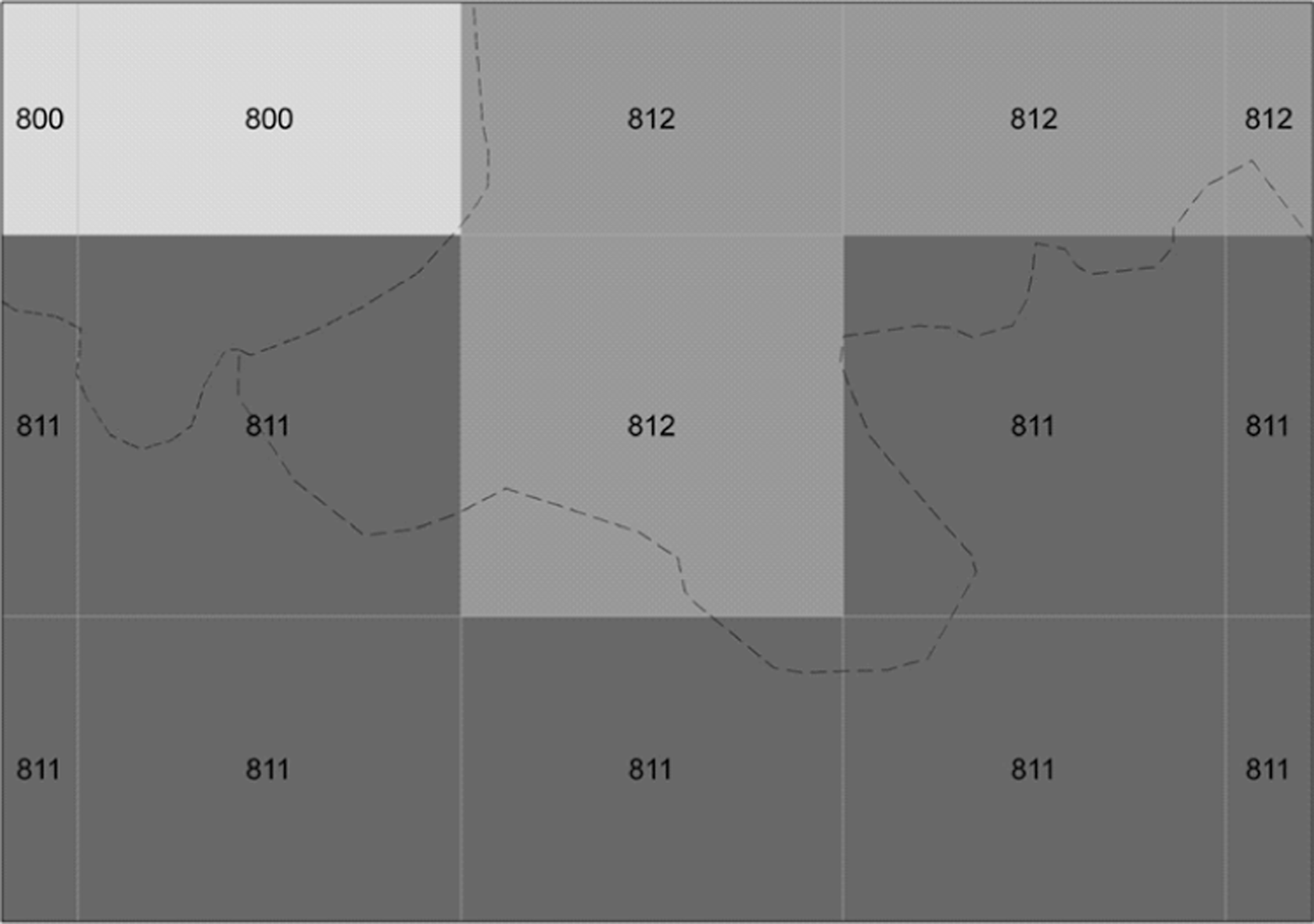
International borders and country assignment
The annual PRIO-GRID files contain a number of time-varying covariates. Among these, we find cell-specific information on the onset and incidence of armed conflicts, represented by a conflict ID variable that corresponds to the case identifier in the UCDP/PRIO Armed Conflict Dataset (Gleditsch et al., 2002; Harbom & Wallensteen, 2010). In case of multiple conflicts within a cell, all conflict IDs are listed in the attribute table. Data on spatial extent of the conflict zones were derived from the affiliated PRIO Conflict Site dataset (Hallberg, 2012). 5 Other data of potential interest to users include various climatic indicators that give cell-specific information on annual temperature and precipitation (see Theisen, Holtermann & Buhaug, 2011/12).
In addition to providing a default set of geo-referenced variables, the PRIO-GRID framework opens for easy expansion to include other GIS data. For example, the Demographic and Health Surveys (DHS) program now routinely registers GPS coordinates for the location of surveyed households. This opens up for generating a host of localized socio-economic indicators, including measures of economic vulnerability and intergroup inequalities (see Østby, Nordås & Rød, 2009).
The PRIO-GRID codebook (Tollefsen, 2012) includes user-friendly instructions on how to adapt and import additional data into the PRIO-GRID structure. Future releases of PRIO-GRID are likely to include a larger range of optional data. Moreover, there are concrete plans to release PRIO-GRID with other resolutions and let the user decide which grid size is more appropriate to her particular research objective. Alternative resolutions also facilitate sensitivity analysis and explicit consideration of possible biases relating to the modifiable areal unit problem (MAUP) and increasing spatial dependence with more refined data (see Openshaw, 1984).
A final benefit of PRIO-GRID is the opportunity to generate country aggregates, weighted by cell area or cell population, for example. While some data are unavailable in a geo-referenced format, the reverse is also true; some data come only as raster or gridded data. For example, there are good daily, monthly, and annual climate statistics at the global level, and measurements of temperature and precipitation are also available as geo-referenced data. However, these data are not released in a country-year format. Figure 4 illustrates how PRIO-GRID may be used to calculate country aggregate area-weighted estimates of total annual precipitation by spatially summarizing a precipitation layer (GPCC, 2010) into a CShapes layer containing the contemporaneous outline of states. Note that large countries, such as Nigeria, have substantial within-country variation in climate, implying that the country average rainfall estimate often is a poor proxy for local climatic conditions.
Aggregation from grid to national-level data
A note on spatial autocorrelation
According to Tobler (1970: 236) ‘Everything is related to everything else, but near things are more related than distant things.’ The assumption of independent and identically distributed (i.i.d.) observations made in inferential statistics often does not hold when working with geographic data. Positive spatial autocorrelation implies that similar values are clustered in space whereas negative autocorrelation denotes a larger heterogeneity in values (checkerboard pattern) than expected by chance. There are various ways to assess the extent of autocorrelation in the data.
A global spatial autocorrelation statistic (e.g. Moran’s I) provides information on the degree of similarity among the observations in the whole study area and is analogous to Pearson’s r. A complementary measure, the local Moran’s I, further reveals where clustering of (dis-) similar attributes are located (Longley et al., 2005).
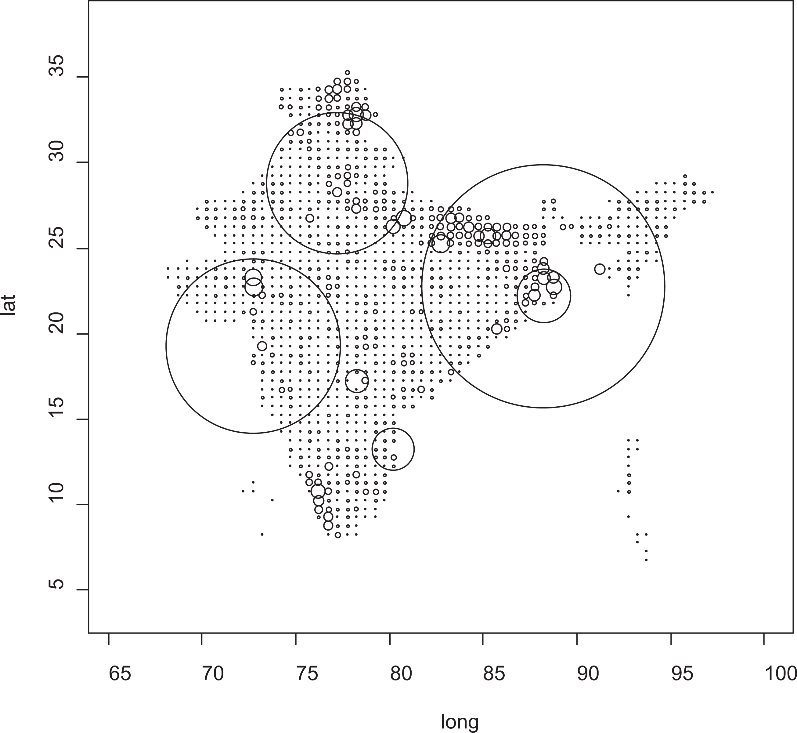
A spatially gridded dataset such as PRIO-GRID inevitably contains indicators with similar values among proximate grid cells. For example, a global Moran’s I test shows that the world’s population is concentrated in a small part of all inhabited land area (I = 0.61). To reveal where high or low values cluster locally we may apply a test for local spatial autocorrelation using the local Moran’s I. This would reveal whether the similarity in neighboring values is greater than what we should expect by chance. Figure 5 illustrates the settlement pattern in India. Unsurprisingly, we find a high degree of spatial clustering in parts of the study area – both highly densely populated areas and areas with scattered populations. The next section illustrates briefly how autocorrelation may bias regression coefficients and how this bias may be corrected.
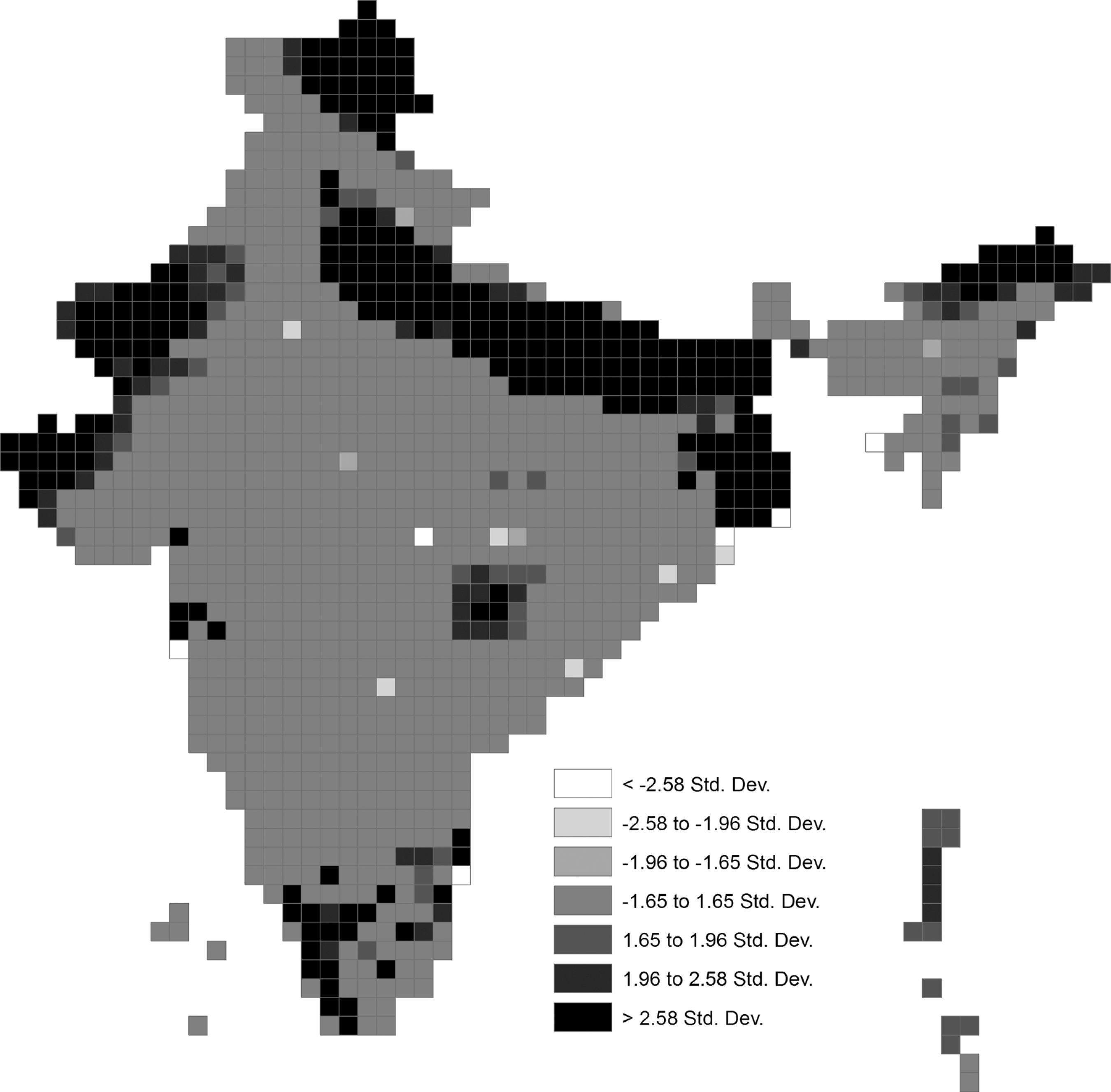
Z-scores from local Moran’s I spatial autocorrelation test
Demonstration of use
As a demonstration of PRIO-GRID, we investigate the spatial relationship between population density and economic activity in India. It is well established that economic development spurs urbanization; in fact, no country has ever experienced sustained economic growth without simultaneous growth in the urban population (UN, 2010). But a reverse effect is also at play: urban areas provide benefits for industries (economies of scale) through agglomeration and complementary services, a large pool of labor, and proximity to markets (Quigley, 1998). Regardless of which direction of causality is more important, we should expect population density and economic activity to be highly correlated in space (Figure 6).
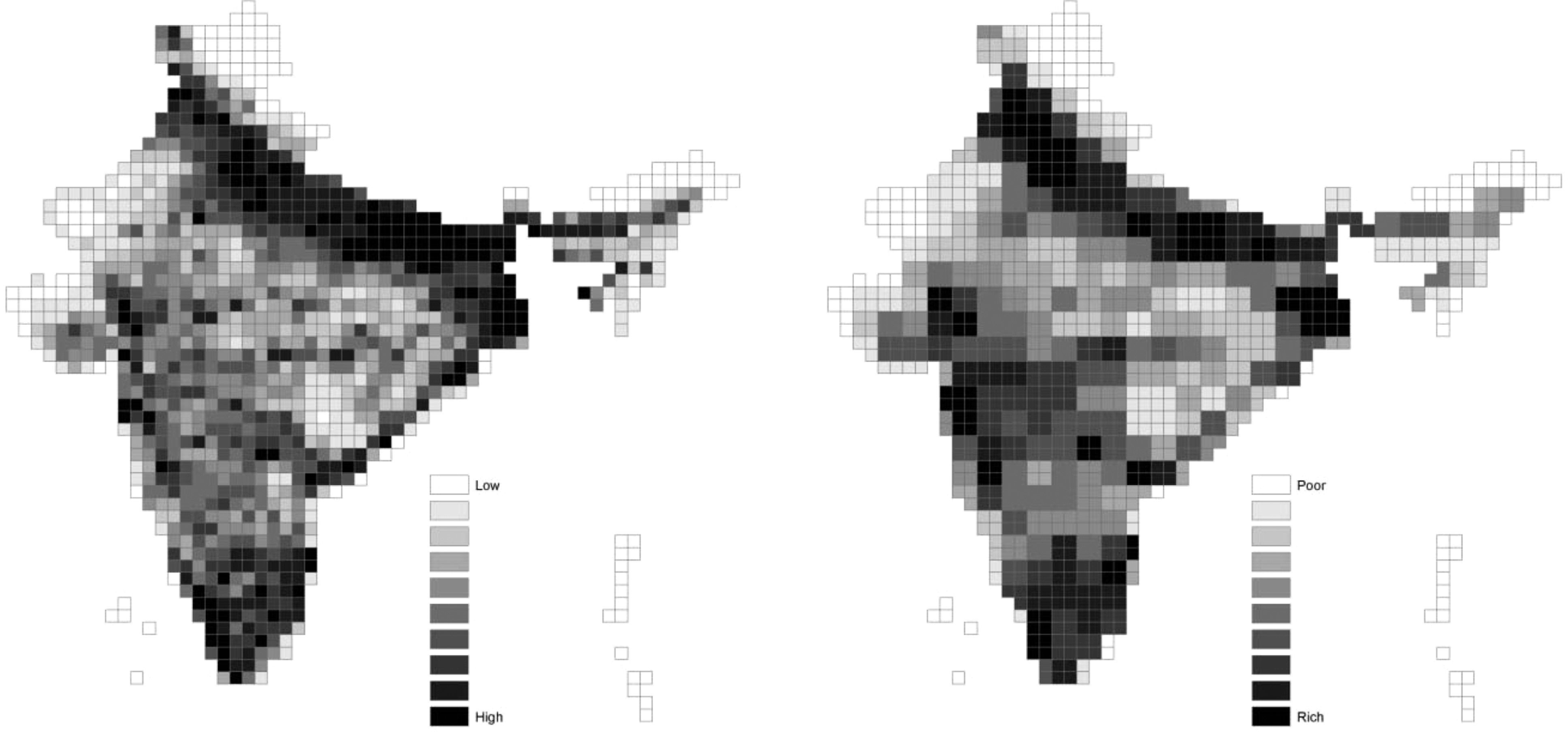
Population density and wealth dispersion in India, 1990
A visual inspection of economic and demographic data for India verifies that areas with high population density overlap with areas with high economic activity. If we want to estimate the effect of population density on local income, then, failing to control for spatial autocorrelation will return biased estimates. To illustrate, we run three simple regression models using the data shown in Figure 6: a naïve OLS model (1), a spatial error model (2), and a spatial lag model (3). All three models use the same dependent variable, PPP-adjusted Gross Cell Product (billion 1990 USD) (Nordhaus, 2006), which is regressed against cell population size (million), population squared, and cell area (1,000 km2). The sample consists of all grid cells in India for a single cross section (1990).
The rationales behind the spatial lag and error models are somewhat different. The spatial lag model assumes that there is a diffusion process where the economic activity of a given cell is dependent on the activity in adjacent cells. The spatial error model is based on an assumption of spatially correlated omitted variables. By decomposing the error term into a spatial part and a unique part, the unique component should be i.i.d. (Ward & Gleditsch, 2008: 39). Although we would have a preference for the spatial lag model in this context, the purpose of this exercise is not to identify key correlates of local economic activity (for which the model clearly is underspecified) but rather to demonstrate how failing to account for correlation structures in the data may bias regression estimates (Table II).
Determinants of local economic activity in India, 1990
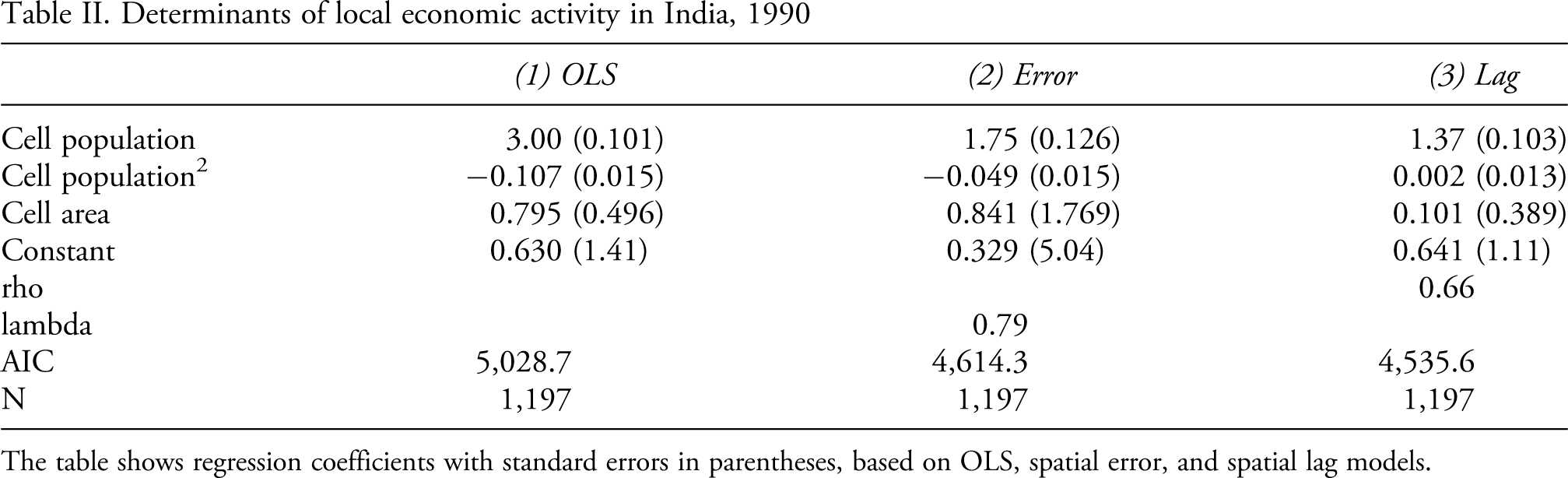
The table shows regression coefficients with standard errors in parentheses, based on OLS, spatial error, and spatial lag models.
All three models in Table II return a positive parameter estimate for population size. The magnitude of this effect varies between the models, however. The naïve Model 1, which completely ignores the spatial clustering in the data, suggests that the isolated effect of local population size on economic activity is quite strong, with an estimated addition of almost $3,000 per extra person in each cell (slightly less than the 2009 Indian average GDP/capita estimate and much more than the 1990 GDP/capita estimate). The spatial error model (2) returns a much more modest effect of almost $1,750 per extra person, which is closer to the 1990 PPP-adjusted average of $1,250. The coefficient for the spatial lag model (3), indicating an increase of $1,370 per extra head, is quite close to the 1990 estimate of GDP/capita for India. However, interpreting the estimate in this manner would imply assuming a constant population effect across space, which we know is not true. The spatial lag not only corrects for spatial interdependence, it also carries an effect onto the interpretation of the model (Ward & Gleditsch 2008: 44ff). When we take the spatial lag into account, we find that the relationship between economic activity and population is estimated to be more or less flat for large parts of the sample. Of the 1,197 cells in the sample, 593 have an estimated effect of less than $10 per extra person, while 750 observations have an estimated effect below $100. Only 106 cells have an estimated effect above the 1990 estimate of GDP/capita of $1,250. For five cells, the estimated effect for each additional citizen is an increase in GCP by more than $10,000. These are the cities of Kolkata (two cells), Delhi, Mumbai, and Madras (Figure 7). 6
Effect of population on economic activity in India, 1990
For more comprehensive empirical assessments using PRIO-GRID, we refer to Buhaug et al. (2011) and Theisen, Holtermann & Buhaug (2011/12).
Conclusion
The quantitative civil war scholarship is gradually recognizing the widespread disconnect between individual- and group-based theories of mobilization and political violence on the one side and country-level empirical analyses of armed conflict on the other. Most civil wars are highly local events and many have little impact on the society at large. Likewise, national data are often poor proxies for the conditions where conflicts occur, and their use may lead to ecological fallacy: inferring about individual behavior from aggregate data. As ever more geo-referenced data and user-friendly GIS applications develop, spatial disaggregation becomes more viable and attractive.
Spatial disaggregation is not without limitations, however. One challenge is the temporal dimension, which is restricted for many types of spatial data (notably for indicators derived from remote sensing); another is the demand for computational power when working with large datasets. Our recommendation is to let the research question and the theoretical approach determine whether gridded data or other subnational research designs are more appropriate than conventional country-level analysis. Accordingly, we offer PRIO-GRID as a supplement to conventional data structures in an effort to facilitate more detailed and spatially sensitive analyses of social phenomena and conditions that cannot be studied at the country level without loss of information.