
Abstract
This article introduces CShapes 2.0, a GIS dataset that maps the borders of states and dependent territories from 1886 through 2019. Our dataset builds on the previous CShapes dataset and improves it in two ways. First, it extends temporal coverage from 1946 back to the year 1886, which followed the Berlin Conference on the partition of Africa. Second, the new dataset is no longer limited to independent states, but also maps the borders of colonies and other dependencies, thereby providing near complete global coverage of political units throughout recent history. This article explains the coding procedure, provides a preview of the dataset and presents three illustrative applications.
In recent years, political science research has increasingly relied on Geographic Information Systems (GIS) as a tool to generate, visualize and analyze spatial data (Gleditsch and Weidmann 2012; Branch 2016). To a large degree, this development has been made possible by the growing availability of geocoded data on political units, actors and events. Contributing to these recent data collection efforts, this article introduces CShapes 2.0, a GIS dataset that maps country borders and capitals from 1886 through 2019. Our dataset builds on the previous CShapes dataset by Weidmann, Kuse, and Gleditsch (2010), which covers independent states from 1946 onward. Compared to the original CShapes dataset, version 2.0 offers two new features: First, it extends temporal coverage by tracing international borders all the way back to 1886, the year that followed the Berlin conference on the partition of Africa. Second, the new dataset is no longer limited to independent states, but also maps the borders of colonies and other dependent territories, thus providing near complete global coverage throughout recent history.
In this article, we compare the key features of CShapes 2.0 with those of other datasets, and describe the main coding decisions and the overall coding process. We also present a number of illustrative applications, using the dataset to examine historical trends in state size, derive population estimates within colonial empires and create a measure of historical border stability to examine its impact on interstate conflict.
Existing Spatial Datasets on Political Borders
Prior to the first release of the CShapes dataset in 2010, most GIS datasets only provided one-time snapshots of country borders, without accounting for border changes over time. Two prominent examples are the Natural Earth Natural Earth (2018) and the GADM boundary datasets (Global Administrative Areas 2012), which map current political borders across the globe. 1 Beyond these “static” data sources, there have also been a few efforts to map historical borders within certain world regions. Most notably, the Euratlas (Nuessli 2010) and the Centennia dataset (Reed 2008) trace political borders in Europe back to 0 AD and 1000 AD, respectively. However, to the best of our knowledge, CShapes to date remains the only available GIS dataset that maps historical borders across the globe.
Despite this key advantage, the original version of CShapes has some limitations. First, its coverage only extends from 1946 to the present. Second, it covers only independent states and excludes colonies and other dependencies, thus not accounting for large parts of the world during the colonial period. This makes the previous version unsuitable for studies that aim for broader global and historical coverage or for research on colonial rule and related topics. CShapes 2.0 addresses these two limitations by backdating borders to 1886, and by mapping colonial dependencies throughout this entire period. Figure 1 illustrates these improvements by comparing a map of Africa in 1946 based on the old and new version of the dataset: Whereas the previous version only contains four polygons for Africa in 1946, CShapes 2.0 covers all fifty-four states and dependencies on the continent.
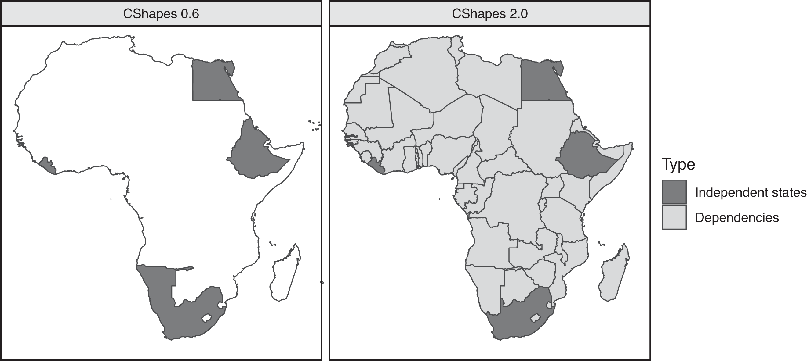
Comparing CShapes 0.6 and 2.0: Africa in 1946.
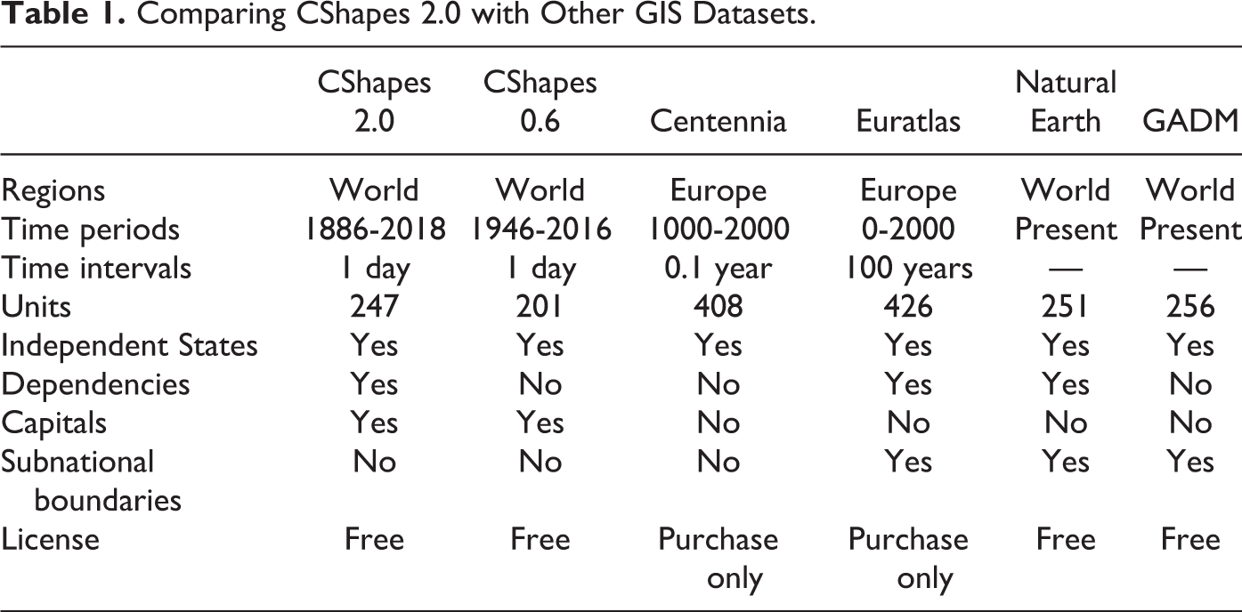
Table 1 summarizes the main differences between CShapes 2.0 and other widely used GIS datasets. Aside from being the only dataset that maps historical borders on a global scale, CShapes also offers a much higher temporal resolution than other historical datasets. For example, Euratlas maps political borders in 100 year intervals, while Centennia uses an interval of ten maps per year. In contrast, CShapes records the exact date of each territorial change and therefore effectively accounts for changes on a daily basis. Moreover, CShapes 2.0 is one of just two datasets that maps the borders of dependent territories over time. 2 Whereas some existing resources such as Euratlas also contain information on cities, CShapes is the only dataset that maps each country’s capital over time. However, it is important to note that CShapes is limited to international boundaries and does not map sub-national administrative boundaries. For the latter, other datasets such as GADM or Euratlas can be used. Lastly, while some datasets such as Centennia or Euratlas require users to purchase a license, CShapes 2.0 is freely available for academic and other non-commercial purposes.
Comparing CShapes 2.0 with Other GIS Datasets.
Coding Procedure
While CShapes 2.0 extends the coverage of its predecessor, it largely retains the data format of previous versions. For the period from 1886 to the present, the dataset represents states and dependencies as GIS polygons. Each polygon is linked to a row in an attribute table that contains further information, such as the time period during which the polygon is active, the territory’s political status and the name and location of its capital. Our representation of countries as time-varying polygons is based on a number of coding rules, which we describe in more detail in the following sections.
Defining States and Dependencies
In order to represent political units in space, we first have to define them. We consider two types of units: independent states and dependent territories. For the former category, most political science research has relied on two main datasets of independent states, each with its own definition of statehood: the Correlates of War (COW) list and the Gleditsch and Ward (1999) list of independent states (GW).
The COW list was first introduced by Russett, Singer, and Small (1968), and covers the period from 1816 to the present. During this period, COW lists all units that qualify as “system members” according to a set of criteria, which include diplomatic recognition by Britain or France in the period before 1920, and membership of the League of Nations or the United Nations in the periods thereafter. In addition, the COW list requires units to exceed a population threshold of 500,000 and also codes states as independent if they maintain diplomatic ties to at least two major powers (Russett, Singer, and Small 1968).
The second major dataset of independent states by Gleditsch and Ward (1999) is derived from COW but uses slightly different criteria: States must have relatively autonomous control over their territory, be recognized by other regional actors and their population must exceed 250,000 during the sample period (Gleditsch and Ward 1999). The GW list mostly covers the same set of states that are listed by COW, but generally uses less restrictive criteria for statehood, and often records much earlier independence dates than COW. For example, COW codes Canada as an independent state from 1920 onward, while GW sets its independence date to 1867. In addition, the GW list offers more expansive coverage of states outside of the European system and includes a number of additional states not listed by COW (for example: Tibet and Orange Free State). 3
Given the widespread use of both datasets in political science, we decided to ensure full compatibility with both the GW and COW list, as done in the previous version. In some cases, this resulted in a complicated double coding scheme, as the two datasets record very different independence dates for several states, in particular during the pre-1945 period. To accommodate these differences, we provide two separate versions CShapes 2.0 that are based either on the COW or GW coding of independent states. 4
Having discussed our coding of independent states, we now turn to their dependencies. We define as dependent territories those units that are under the control of an independent state, but that are not considered part of its core territory. These are typically non-adjacent territories that are ruled as colonies or protectorates. To gather information on dependencies, we rely on a second list of territorial entities, which is also taken from the COW project. The original COW list covered both independent states and other territorial units that were classified as dependencies (Russett, Singer, and Small 1968). These units were later removed from the main COW list, but others have relied on the initial coding to create a separate list of dependencies that extends from 1816 to the present (Wyckoff 1980; Bennett and Zitomersky 1982). Our dataset uses the latest version of this list, which was published as part of the Territorial Change dataset (Tir, Diehl, and Goertz 1998). The coverage of this list ends in 1993. However, this does not constitute a problem for our task, since by then all dependencies had either become part of core states or gained independence, which means they no longer exist as dependent units. While some dependencies continue to exist to the present day (for example, French Polynesia or New Caledonia), no new ones were created after 1993.
For each dependent territory, the COW list of dependencies indicates its political status, as well as the independent state it belongs to. For example, Hawaii is listed as a U.S.-colony from 1898 until 1959, when it became part of the United States. Nigeria is listed as British colony from 1914 until 1960, when it gained independence. 5 Our coding of dependent territories includes the following four categories from the original COW list: (1) colonies, (2) protectorates, (3) international mandates and (4) occupied territories. 6 In cases where a dependent territory gained independence, we code its dependency status up until the date of independence recorded by the COW or GW state list. To ensure consistency with our coverage of independent states, we have narrowed down the list of dependencies to those units with a population greater than 250,000 during the sample period. 7 Figure 2 shows the number of states and dependencies in our dataset over time.
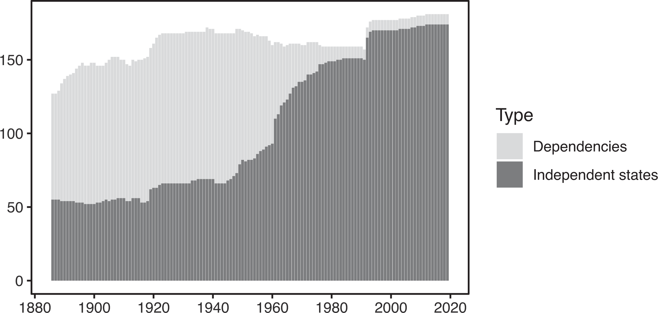
States and dependencies since 1886 (GW-based coding).
The Geographic Extent of States
Having defined the units that make up the international system, our next task is to map their geographic extent. As in the original CShapes dataset, we code a state’s territory primarily based on its internationally recognized boundaries. In most cases, this means that we code borders as they were defined in bilateral and multilateral agreements and shown on contemporaneous maps. One challenge, however, is that some borders lack international recognition or remain disputed. For example, Israel and Syria continue to dispute sovereignty over the Golan Heights, while India and Pakistan remain locked in a dispute over Jammu and Kashmir. In such instances, there may be multiple competing descriptions and maps of the same territories. 8
Instead of coding disputed territories separately, however, we assign them to a given state based on its de facto control over the region. In the case of the Golan Heights, this means that we assign the disputed territory to Israel, although its control over the region is not internationally recognized. In the case of Kashmir, we code the Line of Control as the existing border, although this border remains disputed by both India and Pakistan. In some cases, we lack clear evidence that any state exercised de facto control over a disputed region. The border between Oman and Saudi Arabia is a case in point. This border runs through mostly uninhabited desert land and remained disputed until well into the twentieth century. Negotiations between Britain and Saudi Arabia in 1935 failed, after which both sides continued to make conflicting claims, as shown on contemporaneous maps (Schofield 2016). Saudi Arabia and Oman finally settled on a border agreement in 1990, which closely followed the initial border proposed by Britain (Peterson 2020). Throughout the dispute, we found no clear evidence that either side successfully seized control of the disputed areas. In such instances, we simply backdate borders as they were eventually defined in the agreement that settled the dispute.
Another related issue arises with de facto states, such as Abkhazia and South Ossetia, both of which declared independence from Georgia in the early 1990s, but have not received international recognition. Similar examples include Biafra’s attempted secession from Nigeria in 1967 or the Republic of Serbian Krajina that split from Croatia in 1991. Because these entities do not count as independent states according to our definition, we do not code them as separate units and instead assign their claimed territory to the host state they are located in.
Lastly, an additional challenge in determining the geographic extent of states is that until the early twentieth century, some political units lacked precise borders that enclosed their territories. This was the case especially in parts of Africa, the Middle East and East Asia, where borders long remained poorly defined or non-existent. In these regions, colonial powers and local rulers often gradually defined their borders in successive agreements (Brownlie and Burns 1979). Although we would ideally be able to trace the gradual delineation of borders in these cases, our use of polygons in the dataset does not allow us to do so, since it requires us to represent states as closed spatial units. 9 In cases where state borders remain partially undefined, we therefore add a placeholder polygon that represents the borders as they were eventually defined. These polygons are flagged with a dummy variable to indicate that their borders were not yet fully defined, which enables users to remove or modify these observations if necessary.
Coding Territorial Changes
To account for changes in international borders over time, we need to precisely define what constitutes a territorial change. We distinguish between three types of territorial change, and have systematically gathered data for each type. First, territorial changes may occur due to the creation and dissolution of political units. An example of such a change is the collapse of the Austro-Hungarian empire in 1918 and the subsequent establishment of Austria and Hungary as successor states. A second type of territorial change occurs when states exchange sovereignty over territories as a whole. One example is Germany’s loss of German West Africa (Namibia) to South Africa under the Treaty of Versailles in 1919. In these instances, a territorial unit may change ownership, but its borders remain intact. Thirdly, territorial changes can occur if a part of a country’s core territory is transferred to another country, thus re-drawing the borders between them. An example for this is Germany’s loss of Alsace-Lorraine to France in 1919, which also occurred under the Treaty of Versailles.
To code changes due to the creation and dissolution of units, our coding relies on the GW and COW lists of states and the COW list of dependencies, which we use to track the historical lifespans of political units. For transfers of sovereignty over units as a whole, we also rely on the COW list of dependencies, which keeps track of changes in sovereignty over dependent territories. For border adjustments between existing units, we primarily rely on the Territorial Change Dataset (Tir, Diehl, and Goertz 1998), which lists all territorial transfers since 1816 that involved at least one independent state. For each change, the dataset indicates the gaining and losing side, and provides additional information on the territory that changed hands, such as the territory’s name and its approximate size. For feasibility reasons, we have restricted our coding efforts to transfers of territory larger than 100 × 100 km, as done in the previous version of CShapes. This threshold causes us to exclude a total of 138 smaller territorial changes identified by the Territorial Change Dataset in the post-1886 period. Of these cases, just a few territorial transfers narrowly missed the threshold. For example, Germany gained a total area of 9,702 square kilometers from Poland in 1922 following the Silesia Plebiscite, which is not recorded in our dataset. Similarly, a treaty between Peru and Chile in 1929 awarded an area of 8,498 square kilometers to Chile, which is also not coded. In contrast, one example of a territorial change that narrowly made it into the dataset is Hungary’s annexation of parts of Czechoslovakia in 1938 (11,826 square kilometers). Aside from just a few other close calls, the vast majority of changes that were excluded are either clearly above, or far below the threshold. 10 In addition to excluding territorial changes below the threshold, we also excluded wartime territorial changes, unless they were made permanent in treaties signed after the war. 11 In the latter case, we relied on the date of postwar agreements as the date of the change.
One limitation of the Territorial Change Dataset is that it only records changes involving independent states according to the COW definition. This excludes potential border changes between units that do not qualify as independent states according to COW. To address this, we gathered additional information, relying mainly on the Encyclopedia of International Boundaries by Biger (1995) and another encyclopedia of African Boundaries by Brownlie and Burns (1979). Both sources provide extensive coverage of border changes that include the colonial period and give detailed accounts of each change and the location of borders thereafter. In keeping with the coding rules of the Territorial Change Dataset, we used the precise date of treaties that confirm the reallocation of territory as the date of each change.
Geocoding
Using the information described in the previous section, we created a comprehensive list of all relevant territorial changes since 1886. This list served as basis for the identification of country periods during which the political status, the capital and borders of a territory remain unchanged. Conversely, any change in one of these attributes marks the beginning of a new period. After defining all country periods, we gathered detailed information on the location of territorial transfers, and on the historical circumstances under which each change took place. This information is summarized in our dataset’s documentation, which provides a detailed chronology of territorial changes per country and discusses our coding decisions in a number of ambiguous cases.
Our coding of country periods supported the collection of historical maps that depict the status quo of borders before each change. Figure 3 shows an example of such a map depicting borders in Europe in 1936. We geo-referenced these maps using GIS software and used them to draw and modify country borders. Border changes were coded in reverse chronological order. In other words, we started with the earliest observation in the original CShapes dataset, and adjusted country polygons to represent borders before each territorial change. 12 For countries that did not experience any changes in the previous period, such as Switzerland or Portugal, we simply backdated their borders to 1886. In cases where changes did occur, such as the border between France and Germany in 1919, we adjusted those portions of the border affected by each change in reverse chronological order.
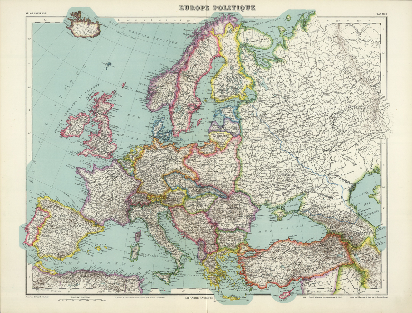
Map of Europe in 1936 used to code country borders (Vivien de Saint-Martin and Schrader 1937).
The final dataset covers 249 political units that are represented by 476 polygons over time. 152 countries have a single polygon during the entire period, while 97 countries have two or more. In total, our dataset covers 357 territorial changes. Of these changes, 159 are due to the creation and dissolution of units. 112 changes are transfers of sovereignty over dependent territories, for example due to the independence of former colonies. Lastly, 86 changes are boundary adjustments between existing units. Figure 4 gives a preview of our data, showing the changing political map of Southeast Europe between 1886 and 1946. 13
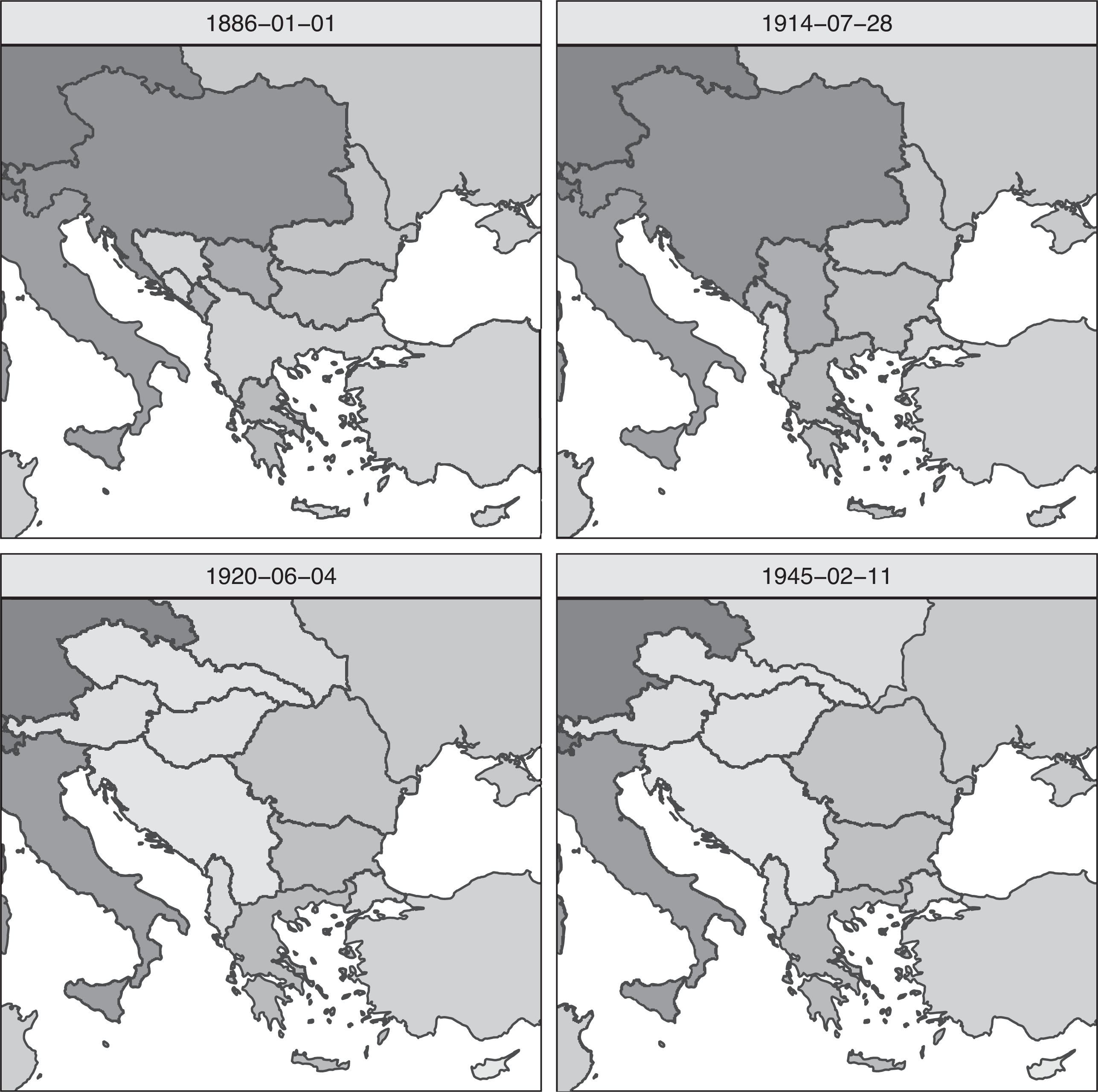
Border changes in Southeast Europe 1886-1946.
Applications
What can we learn from our new dataset? In this section, we present three illustrative applications: First, we examine general trends in state size since 1886. Second, we illustrate how CShapes 2.0 can be combined with other spatial datasets to compute new variables. Lastly, we use our data to derive a new indicator of border stability over time, and examine its relationship with interstate conflict. 14
Examining Trends in State Sizes
We begin with the question of state size, which has been the subject of a long-standing debate (Friedman 1977; Tilly 1990; Alesina and Spolaore 2003; Lake and O’Mahony 2004; Abramson 2017). While this debate has remained largely theoretical, a few studies have also examined the evolution of state sizes empirically. For example, Lake and O’Mahony (2004) estimate state sizes from 1816 to the present and find that the average state’s size increased until the late nineteenth century, after which it dropped continuously until the present. In contrast, a recent study by Abramson (2017) examines state sizes in Europe between 1100 and 1790, showing that most states decreased in size throughout this period.
To shed more light on this question, we use the CShapes dataset to examine historical trends in state size. Our analysis starts in 1886 and therefore covers most of the period studied by Lake and O’Mahony (2004). Following this study, we focus on independent states and define their territories based on their “core” areas, thus excluding colonial holdings overseas. Based on our coding of country borders, we calculated the average size of states in each year, as shown in Figure 5. The results show that state sizes initially increased throughout the 1890s and peaked in 1901, followed by a slight decline. After a renewed increase up to 1919, state sizes sharply declined until the present. In 2019, the average state was less than half the size of its counterpart in 1901.
This downward trend in state size, which matches Lake and O’Mahoney’s findings, could be driven by two separate developments. On the one hand, it may be the result of states losing parts of their territory or breaking up into multiple successor states, as happened in the case of Yugoslavia. On the other, the decrease could also be due to the large number of colonies that joined the club of independent states after World War II. Most colonies existed throughout the twentieth century with identical borders and were generally smaller than the average sovereign state. Therefore, the sharp decline in state size could be the result of a growing community of independent states rather than the actual “shrinking” of existing territorial units.
Lake and O’Mahoney discuss both possibilities and conclude that the overall trends in state size are mostly driven by changes in state borders rather than state birth or death. To support this claim, they show that the average size of new states has decreased consistently since 1816. However, while this trend indeed contradicts the nineteenth century increase in state size, it is still compatible with the twentieth century decline. More generally, it is unclear whether the average size of new states can account for the general trend, given that state births are quite rare and tend to cluster in certain historical periods. Using the new CShapes dataset, we adopt a more straight-forward approach that calculates the average size of any territorial unit (i.e. both independent states and colonial dependencies) across time. This combined measure enables us to rule out changes in average state size that were due to decolonization, as our dataset covers former colonies both before and after independence. The results, shown by the dotted line in Figure 5 point to a less conclusive trend. Although we still see a drop in state sizes following World War I and the Cold War, the average size of states remained mostly constant and even increased slightly between 1920 and 1965. This suggests that the sharp decline in state sizes after World War II was mostly the result of decolonization, rather than the widespread redrawing of boundaries. Still, even our combined measure shows that states today are smaller than they were in the early twentieth century owing to border change and territorial losses.
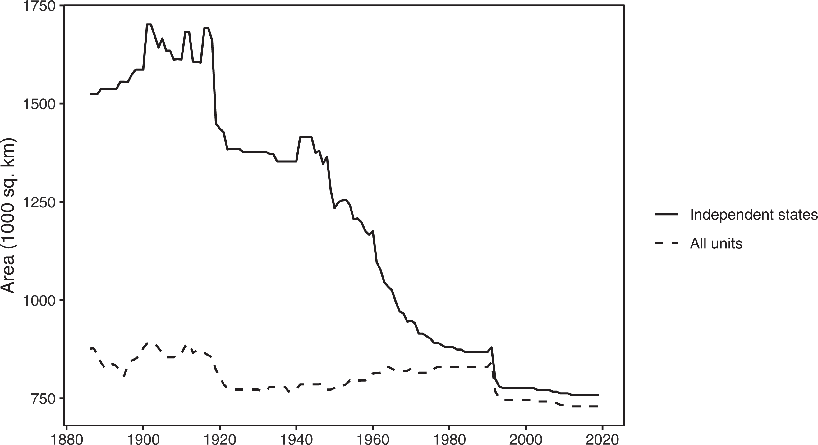
Average state sizes over time.
Spatial Population Estimates
In our second example, we use the CShapes polygons to compute historical population estimates for colonies. Population estimates are widely used in cross-country analyses, but existing datasets usually provide such estimates exclusively for independent states (e.g. Gleditsch 2002). In order to estimate the population within colonies over time, we use gridded population data from the HYDE database (Klein Goldewijk et al. 2011). The HYDE data provide historical population estimates measured within 5’ × 5’ grid cells, which are coded in ten year intervals since 1700. 15 We use population grids from 1890 to 2010, which we overlay with CShapes polygons at each point in time. We then use our country polygons as “cookie cutters” to extract and summarize population values within each country’s borders, as illustrated in Figure 6. For the purpose of this illustration, we calculate the total population within all British, French and other colonies across time. Our estimates show that from 1890 to 1940, the British colonial empire had a total population that was more than twice as large as all other colonial empires combined. At its peak, nearly 25 percent of the World’s population was part of the British empire, according to our spatial estimates. Following World War II, the total population within the British empire declined rapidly as a result of decolonization, followed by a similar decline among French and other colonies.
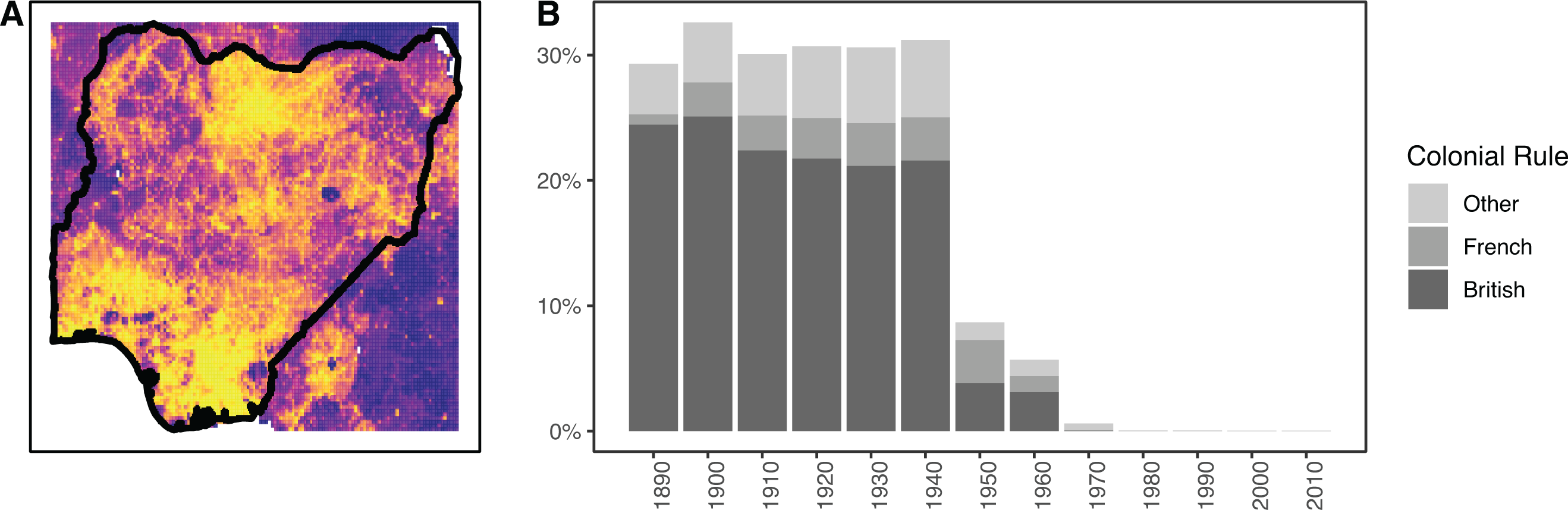
Computing historical population estimates. (A) Overlaying population data with CShapes polygons. (B) Estimated share of world population under colonial rule since 1890.
Border Age and Conflict Risk
In our third application, we illustrate how new variables derived from the dataset itself can also help to address important questions in conflict research. In this particular example, we explore how the historical stability of international borders affects the risk of interstate conflict. Previous research has highlighted the important role that borders play in coordinating interstate relations by clarifying the limits of state sovereignty and jurisdiction. According to this view, settled borders reduce uncertainty in international politics and create favorable conditions for economic exchange and cooperation between neighboring states. As states and local populations coordinate on existing borders, this is expected to increase the costs of conflict (Simmons 2005; Carter and Goemans 2011, 2014; Schultz 2015). Therefore, we may expect the risk of conflict between neighboring states to decrease over time, the longer their borders have remained in place.
We test this idea in an analysis at the level of border segments, which we derive from the CShapes 2.0 dataset. More precisely, we convert our time-varying country polygons into dyadic land borders, and then split these borders into 100 km segments that serve as our unit of analysis. To capture interstate conflict as our outcome variable, we use geocoded data on Militarized Interstate Dispute (MID) events from the MIDLOC dataset (Braithwaite 2010). Our analysis is limited to the period from 1993-2001, as MIDLOC only provides full coverage of MID events during this period. We define 20 km buffer zones around each border segment and assign MID events to a border segment if they fall within the segment’s surrounding buffer zone. 16 We then estimate a simple negative binomial model that uses the total number of MID events near each border segment as the dependent variable. Our main explanatory variable is a logged measure of the age of the border segment at the beginning of our period of observation. As control variables, we include logged measures of terrain ruggedness and population density, which are measured within a buffer zone around each border segment, as well as a logged measure of the total area of each buffer zone. Our model also features a dummy variable for borders drawn under colonial rule and for borders that belong to a democratic dyad. Finally, our specification includes a logged measure of each dyad’s age in years.
The results of our analysis are shown in Table 2. Model 1 only includes the explanatory variable, while Model 2 adds our controls. In both models, we find that MID events are less frequent nearby long-established border segments than around more recently established borders, which is in line with our hypothesis. These findings are of course only suggestive, as our analysis does not fully account for endogeneity and omitted variables. 17 However, our results are consistent with previous studies, which have shown that regions with historically unstable borders are more vulnerable to border disputes (Abramson and Carter 2016) and that new international borders tend to become less conflict-prone as time passes (Carter and Goemans 2014). While the latter study finds that this effect is limited to borders that are based on previous administrative boundaries, our results suggest that the positive effects of border stability may apply to any type of international boundary.
Count Models: MID Events (1993-2001).
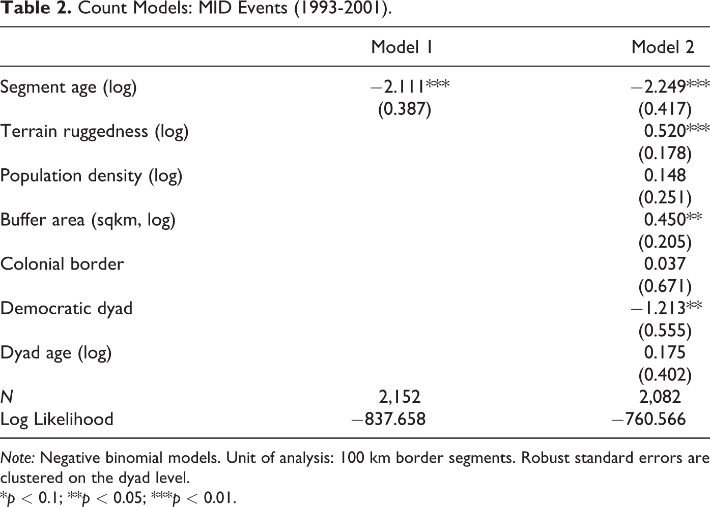
Note: Negative binomial models. Unit of analysis: 100 km border segments. Robust standard errors are clustered on the dyad level.
*p < 0.1; **p < 0.05; ***p < 0.01.
The cshapes R Package 2.0
CShapes 2.0 also comes with an updated R package called cshapes that allows users to take advantage of our dataset even if they lack specialized GIS skills. The package gives users access to the latest version of our dataset that covers country borders from 1886 to the present, and includes functions that enable users to extract data on country borders at any point in time during that period. These functions can be used to create historically accurate maps and to compute various between-country distance measures that are commonly used in statistical applications. Furthermore, the new package no longer relies on R’s sp standard for spatial data, but instead uses the new simple features (sf) data representation, which is intended to replace sp and is generally more user-friendly (Pebesma 2018). The new cshapes R package and future updates is distributed using the Comprehensive R Archive Network (CRAN).
Conclusion and Outlook
In this article, we have introduced CShapes 2.0, a GIS dataset that maps the borders and capitals of states and dependent territories from 1886 to the present. To our knowledge, CShapes 2.0 is the only GIS dataset that keeps track of historical border changes on a global scale and offers a much higher temporal resolution than other historical GIS datasets. Using CShapes does not require specialized GIS skills, as the accompanying R package makes it easy to produce historically accurate maps and to compute between-country distance measures. Unlike other historical GIS datasets, CShapes 2.0 is available free of charge for academic and other non-commercial purposes. In three illustrative applications, we have shown how the new data can be used to examine trends in state size and to produce spatial estimates of populations under colonial rule. We have also examined the relationship between the age of a border and the risk of interstate conflict, finding that the likelihood of militarized conflict between neighboring states decreases the longer their borders have remained in place. Beyond these specific examples, we believe that CShapes 2.0 will enable new research on a broad range of topics that have proven difficult to study so far. Among many others, these include historical processes such as state formation, the expansion of colonial rule, the long-term impacts of conquest and border change and potential legacy effects of historical boundaries in Europe, Asia and beyond. By mapping political units throughout recent history, we hope to contribute to a better understanding of these questions.
Supplemental Material
Supplemental Material, sj-pdf-1-jcr-10.1177_00220027211013563 - Mapping the International System, 1886-2019: The CShapes 2.0 Dataset
Supplemental Material, sj-pdf-1-jcr-10.1177_00220027211013563 for Mapping the International System, 1886-2019: The CShapes 2.0 Dataset by Guy Schvitz, Luc Girardin, Seraina Rüegger, Nils B. Weidmann, Lars-Erik Cederman and Kristian Skrede Gleditsch in Journal of Conflict Resolution
Supplemental Material
Supplemental Material, sj-zip-1-jcr-10.1177_00220027211013563 - Mapping the International System, 1886-2019: The CShapes 2.0 Dataset
Supplemental Material, sj-zip-1-jcr-10.1177_00220027211013563 for Mapping the International System, 1886-2019: The CShapes 2.0 Dataset by Guy Schvitz, Luc Girardin, Seraina Rüegger, Nils B. Weidmann, Lars-Erik Cederman and Kristian Skrede Gleditsch in Journal of Conflict Resolution
Footnotes
Declaration of Conflicting Interests
The author(s) declared no potential conflicts of interest with respect to the research, authorship, and/or publication of this article.
Funding
The author(s) disclosed receipt of the following financial support for the research and/or authorship of this article: This work was supported by the Swiss National Science Foundation (156339) and the European Research Council (ERC Advanced Grant 787478).
Supplemental Material
Supplemental material for this article is available online.
Notes
References
Supplementary Material
Please find the following supplemental material available below.
For Open Access articles published under a Creative Commons License, all supplemental material carries the same license as the article it is associated with.
For non-Open Access articles published, all supplemental material carries a non-exclusive license, and permission requests for re-use of supplemental material or any part of supplemental material shall be sent directly to the copyright owner as specified in the copyright notice associated with the article.