Sage Journals: Discover world-class research

Abstract

A numerical methodology is proposed to determine the 3D failure criteria of directional composite joints, accounting for both in-plane (in-/off-axis) and out-of-plane behavior. The approach involves simulating standard composite joint characterization tests using a high-fidelity, three-dimensional finite element damage modeling strategy. A simplified modeling strategy to simulate multi-bolt joints is then proposed: the joints are simulated using a combination of linear-elastic multilayer composite shell elements and connector elements, which fail once their internal forces intercept the previously determined 3D failure envelope. The methodology is applied to five multi-bolt single lap shear geometries and the results are compared with those obtained using high-fidelity simulations. Results indicate that the methodology developed to numerically determine the bolt failure envelope, combined with the use of connector elements as fastener representatives, is appropriate to accurately simulate the joint stiffness and load ratios in the first failed bolt, and predict first-drop laminate-level failure in composite bolted connections while providing a substantial reduction in computation expenses, establishing their potential for future use in large-scale models.

Keywords

composite materials finite element analysis bolted joints failure criteria

Introduction

The numerical modeling of composite bolted structures can be approached with varying levels of complexity. Three-dimensional solid models that combine ply-by-ply simulation of the laminate and 3D representation of the fastener and washers have been found to provide the most accurate failure predictions of bolted joints, but the computational and data burden associated with these simulation strategies constitute a major drawback.^1–9 In fact, while these high-fidelity 3D numerical models have recently been shown to provide accurate failure load predictions of composite bolted connections loaded in pure loading conditions^10–16 and in mixed-mode conditions,¹⁷ providing an alternative to the high cost and wasteful characterization of these joints, they are still limited to coupon size tests, and, therefore, are not ideal for the design of large structures.

The simplification of 3D solid bolted joints has been investigated by several authors,^{1,4,6,9,18,19} as discussed below, where different proposed solutions are described giving particular emphasis to those implemented in the finite element software Abaqus. The use of connectors, elements designed to link two nodes or surfaces (based on kinematic relationships) with local relative displacements and rotations, has been widely reported as an efficient alternative to the 3D solid representation of the bolts. The greatest challenge related to the replacement of fully 3D bolts by connectors is the need for an a priori definition of the element’s flexibility. While connector stiffness equations which relate the substrate stiffness, thicknesses, and bolt geometry to the bolt flexibility have been proposed by several authors, e.g. Huth,²⁰ Grumman,^21,22 Tate & Rosenfeld,^21,22 Swift,²² and Boeing’s first and second equations,^21,23 the selection of which equation to use in each application seems to mostly rely on a calibration procedure. For example, Eremin et al.²¹ illustrated a comparison between the different connector stiffness equations listed above. For both composite-composite and composite-metal connections, Huth’s formula²⁰ was found to be the most suitable for large-thickness laminates, while the first Boeing equation²¹ is the most adequate for small and medium-thickness plates. More recently, Chandregowda and Reddy²² demonstrated that the most accurate fastener flexibility and load distribution can be achieved for Abaqus built-in bushing connectors using Huth’s²⁰ or Grumman’s^21,22 equations.

Regarding higher-complexity connector-based strategies, Verwaerde et al.⁶ developed and validated a novel non-linear connector model in a large-scale turbine casing with good results. In a subsequent study, the same authors⁹ introduced a variation of the connector model with non-linear frictional behavior and applied it in the study of an industrial-scale manifold assembly with a significant reduction in run time.⁹ These developments confirm the adaptability, flexibility and tailoring potential of connectors.

Other simplified approaches to simulate bolted joints have also been presented by Tanlak et al.,¹⁸ who proposed several models employing different combinations of deformable and rigid shell elements, Timoshenko beams, and connector beams, for comparison against a fully-solid bolted joint under impact loading. After employing these alternatives in a full model, an overall saving of 80–90% of computational time was obtained using the same mesh density. Kim et al.⁴ suggested four different solid-laminate bolt models. Although the solid bolt model predicted the structural behavior with the highest level of accuracy, the coupled bolt model and the spider bolt model, both represented by beam elements in different configurations, greatly reduced computational time and memory usage. An alternative approach was investigated by Sharos and McCarthy,¹⁹ who developed a spring model, with a 2-node user-defined element suitable for explicit simulations (VUEL) with 5 degrees of freedom (DOFs) per node, with excellent correlation for both bearing load and out-of-plane displacement. Gray and McCarthy¹ also presented a global bolted-joint model (GBJM) using master node couplings between beam and analytical rigid body elements, capable of accurately reproducing the results obtained with full 3D models.²⁴

In addition to allowing the prediction of the stiffness of composite bolted connections, these simplified models can be endowed with failure criteria to predict the structural integrity of the large-scale structure. The failure criterion can be applied in-model³ or as a post-processing step. For the former, once the failure load is reached, the load-carrying capability of the element is instantly reduced to zero, and the element is removed. In the latter case, failure criteria are applied after running linear elastic simulations, and failure is determined by analyzing the bolt loads a posteriori. Regardless of the way bolt failure is considered in these simplified models, the joint failure load must be determined, and therefore, composite joints at the coupon level must be tested to estimate the failure load of the whole joint. Characterizing the behavior of composite bolted joints typically involves determining their load resistance under bearing (in-plane) and pull-through (out-of-plane) conditions, in compliance with the ASTM standards 5961²⁵ and 7332,²⁶ respectively. Composite joints are generally designed to fail under shear, and thus the most relevant value to obtain is the in-plane bearing load.²⁵ However, depending on their application, joints typically experience a combination of loading conditions rather than exclusively pure-mode loads, which subject the bolts to both in-plane and out-of-plane stresses.

Recently, and following this need to characterize composite joints in more realistic loading scenarios where combined loadings are present (e.g. L-junctions and single-lap shear joints), an experimental methodology was developed to extend this characterization to mixed-mode loadings, where a controlled ratio between pull-through and bearing loads is applied to a quasi-isotropic laminate.¹⁷ This new technique allowed the determination of a failure envelope of the bolted joint which can be used for the design of larger scale structures, e.g. using simplified connector-based models with embedded bolt failure criteria. This characterization becomes even more relevant for directional laminates, where an off-axis in-plane load will lead to a different joint performance, as opposed to quasi-isotropic systems. While in Ref. 17 a 2D bearing/pull-through envelope was sufficient for the characterization of quasi-isotropic specimens, a 3D failure envelope is required for an adequate assessment of directional samples to account for their anisotropic in-plane behavior.

Building on previous research by Furtado and several co-authors of the present paper,¹⁷ we extend this concept by introducing a numerical approach to determine the 3D failure criteria of a directional composite joint, considering its in-plane (in-/off-axis) and out-of-plane behavior. The proposed approach leverages the high-fidelity numerical simulation strategy developed and validated previously. The 3D failure envelope is used as a post-processing predictive tool in four simplified multi-bolt single-lap-shear models, for the estimation of bolt load ratios, failure loads, and stiffness values. A comparison is then drawn between the outcomes predicted by the developed approach and the results obtained from their corresponding high-fidelity simulations. The comparison reveals excellent agreement in terms of joint stiffness and bolt load ratios (differences below 5.6% and 10.8%, respectively) and a satisfactory match in failure loads (average error of 18.4%). Notably, the simplified methodology achieves these results while reducing computational time by a factor of more than 500 times. Further refining the simplified modeling strategy and failure ellipsoid calculation would improve the accuracy of the proposed methodology and affirm its suitability for the stress analysis of large composite structures.

Three-dimensional failure envelope of a directional laminate

In Ref. 17, a two-dimensional combined bearing/pull-through failure envelope was experimentally determined for a quasi-isotropic carbon-fiber-reinforced polymer laminate (Hexcel’s IM7/8552) using an experimental test rig detailed in Appendix A. By numerically reproducing the experimental tests of bolt-bearing,²⁵ pull-through,²⁶ and combined loading¹⁷ using high-fidelity 3D models defined in Abaqus, the numerical failure envelope was determined with acceptable deviations from the experimental results (between approximately −10% and 10%), thus validating the numerical approach for the characterization of bolted joint failure envelopes. Here, this numerical strategy to determine composite joint failure envelopes is extended for the prediction of the behavior of directional laminates. Due to their anisotropic nature, oriented laminates exhibit different bearing resistance values depending on the in-plane shear loading direction, displaying a greater stiffness and strength along their primary axis. Thus, a three-dimensional failure envelope is required for their full characterization.

The three-dimensional failure envelope is defined here through the same validated numerical methodology. The damage and failure modeling strategy for the bolt-bearing, pull-through and combined bearing/pull-through models follows Ref. 17. As the model definition is not the main contribution of this work, details regarding its design, based on experimental configuration, are presented in Appendix A.

Modeling strategy

The high-fidelity models illustrated in Figure 1 represent the six load scenarios considered here. The load ratio η, defined as η = P_B/(P_B + P_PT) (where P_B and P_PT represent the bearing and pull-through loads, respectively), assumes values of 0.2, 0.4, 0.6 and 0.8, ranging from higher out-of-plane loads to higher in-plane loads, by varying the dimensions of the loaded rig component of the combined-loading model, as described in Appendix A.

Figure 1.

High-fidelity models with η ratios ranging from 0 to 1. For a clearer visualization, the rig and block parts of the pure pull-through and pure bearing models, respectively, are represented with a mid-plane cut.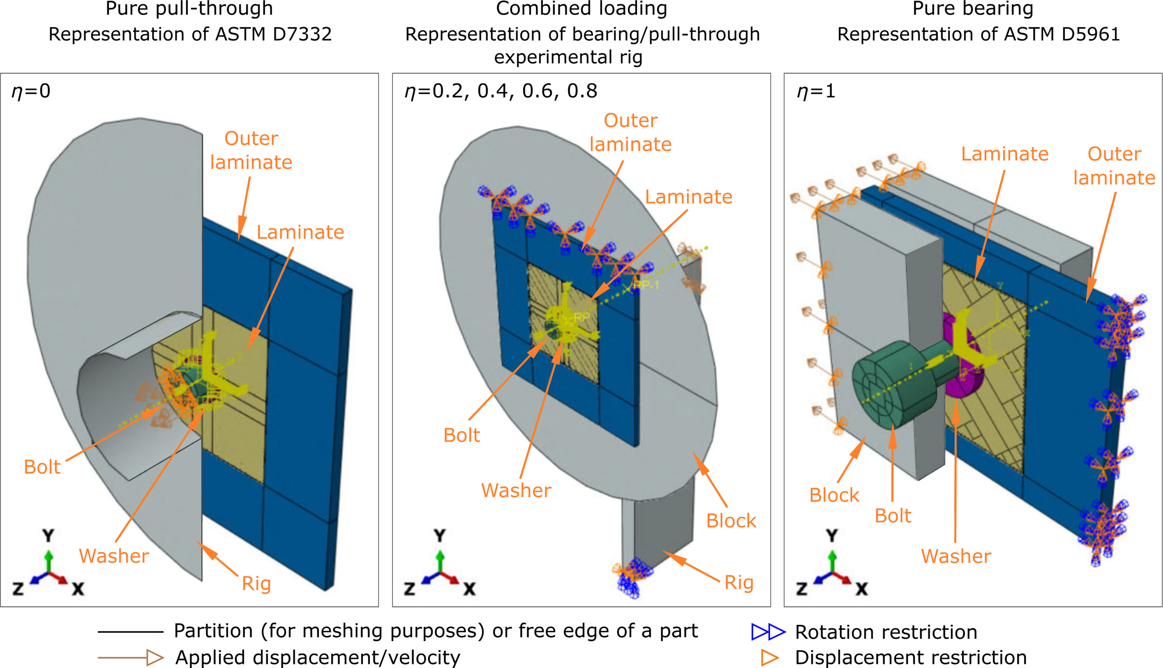

The pure bearing model, corresponding to η = 1, was designed in compliance with the ASTM D5961 standard²⁵ and is represented by a double-lap shear configuration, which includes two blocks connected to either side of the laminate to constrain the bolt movement along the length of the specimen (x-axis). The pure pull-through model, in turn, corresponds to η = 0 and is similar to the combined-loading model, but excludes the rig component. Instead, the displacement is applied directly to the bolt along the z-axis, to meet the requirements of the ASTM D7332 standard.²⁶

Both pure and combined-loading numerical models employ a meso-scale numerical approach, where each ply is explicitly modeled using solid elements and connected to adjacent plies by cohesive elements. The constitutive model used for the plies is the smeared crack model proposed by Camanho et al.,²⁷ which is capable of predicting the onset and propagation of intralaminar damage, and delamination is simulated using a frictional cohesive zone model.^28–30

In all models, the damageable plies are connected to an outer linear elastic laminate, modeled with a coarser mesh to reduce computation time, through Abaqus tie constraints. Surface-to-surface contact with frictional tangential and “Hard” normal behaviors was applied between each contacting part. All bolted assemblies were simulated with a 2.2 Nm torque by applying a temperature differential to the washer, causing it to expand and pretension the bolt, compressing the laminate.

A more detailed explanation of the numerical procedure, including further information on the modeling strategy for an accurate representation of the experimental rig and the constitutive models used for all high-fidelity models, can be found in Appendix A.

Loading case definition

The high-fidelity models were used to simulate a total of 18 loading cases with varying bearing/pull-through ratios and bearing load directions for a directional, symmetric [45/90/−45/0/0/45/0/0/−45/0]_S laminate manufactured in Hexcel’s IM7/8552 carbon fiber/epoxy material with a cured ply thickness of 0.125 mm.

Combined-model simulations for four load ratios (0.2, 0.4, 0.6 and 0.8) were run in conjunction with the pure bearing and pure pull-through models, totaling six simulations for the longitudinal bearing analyses (0° fibers aligned with the bearing loading direction) and six simulations for the transversal bearing analyses, performed by rotating the entire laminate 90°. The connection between the longitudinal and transversal bearing cases was determined by rotating the pure bearing laminate 30° and 60°. Similarly, and to increase fitting accuracy, the points enclosed amidst the failure envelope were obtained through a laminate rotation of 45° on the combined loading model, and the projection of the peak loads onto the two bearing axes. Table 1 presents the final layups after rotation alongside their respective load ratios.

Table 1.

Directional layups and respective loading conditions. In the “plane” column, “LB” designates longitudinal bearing, “TB” represents transversal bearing, and “PT” stands for pull-through.

Rotation angle	Layup	Load ratios	Plane
Original layup	[45/90/−45/0/0/45/0/0/−45/0]_S	0.0, 0.2, 0.4, 0.6, 0.8, 1.0	LB/PT
30°	[75/−60/−15/30/30/75/30/30/−15/30]_S	1.0	LB/TB
45°	[90/−45/0/45/45/90/45/45/0/45]_S	0.2, 0.4, 0.6, 0.8	—
60°	[−75/−30/15/60/60/−75/60/60/15/60]_S	1.0	LB/TB
90°	[−45/0/45/90/90/−45/90/90/45/90]_S	0.0, 0.2, 0.4, 0.6, 0.8, 1.0	TB/PT

Failure load predictions

The failure load predictions obtained at the first significant load drop (

>

10%) are listed in Table 2, and the load-displacement curves for three representative load ratios (η = 1.0, 0.8, 0.0) are displayed in Figure 2. For completeness, the curves for the remaining ratios are illustrated in Figures SI.1a to SI.1c of the supplemental material. The curve is shown up to the point where the simulation ended due to numerical errors related with excessive element distortions. Importantly, in all cases, the first load drop was successfully obtained, even though the load pickup was not achievable in every simulation. As the analysis presented here focuses specifically on the first load drop, this method aligns with the primary objective of the study. A considerable difference in stiffness can be observed between the pure bearing cases, due to the different load-bearing contributions of the different ply orientations. When the load is aligned along the laminate’s principal orientation, the 0° plies promote greater stiffness. As pull-through loads become more prevalent, the discrepancy in stiffness is minimized.

Table 2.

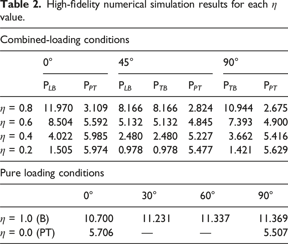
High-fidelity numerical simulation results for each η value.

Combined-loading conditions
	0°		45°			90°
	P_LB	P_PT	P_LB	P_TB	P_PT	P_TB	P_PT
η = 0.8	11.970	3.109	8.166	8.166	2.824	10.944	2.675
η = 0.6	8.504	5.592	5.132	5.132	4.845	7.393	4.900
η = 0.4	4.022	5.985	2.480	2.480	5.227	3.662	5.416
η = 0.2	1.505	5.974	0.978	0.978	5.477	1.421	5.629

Pure loading conditions
	0°	30°	60°	90°
η = 1.0 (B)	10.700	11.231	11.337	11.369
η = 0.0 (PT)	5.706	—	—	5.507

Figure 2.

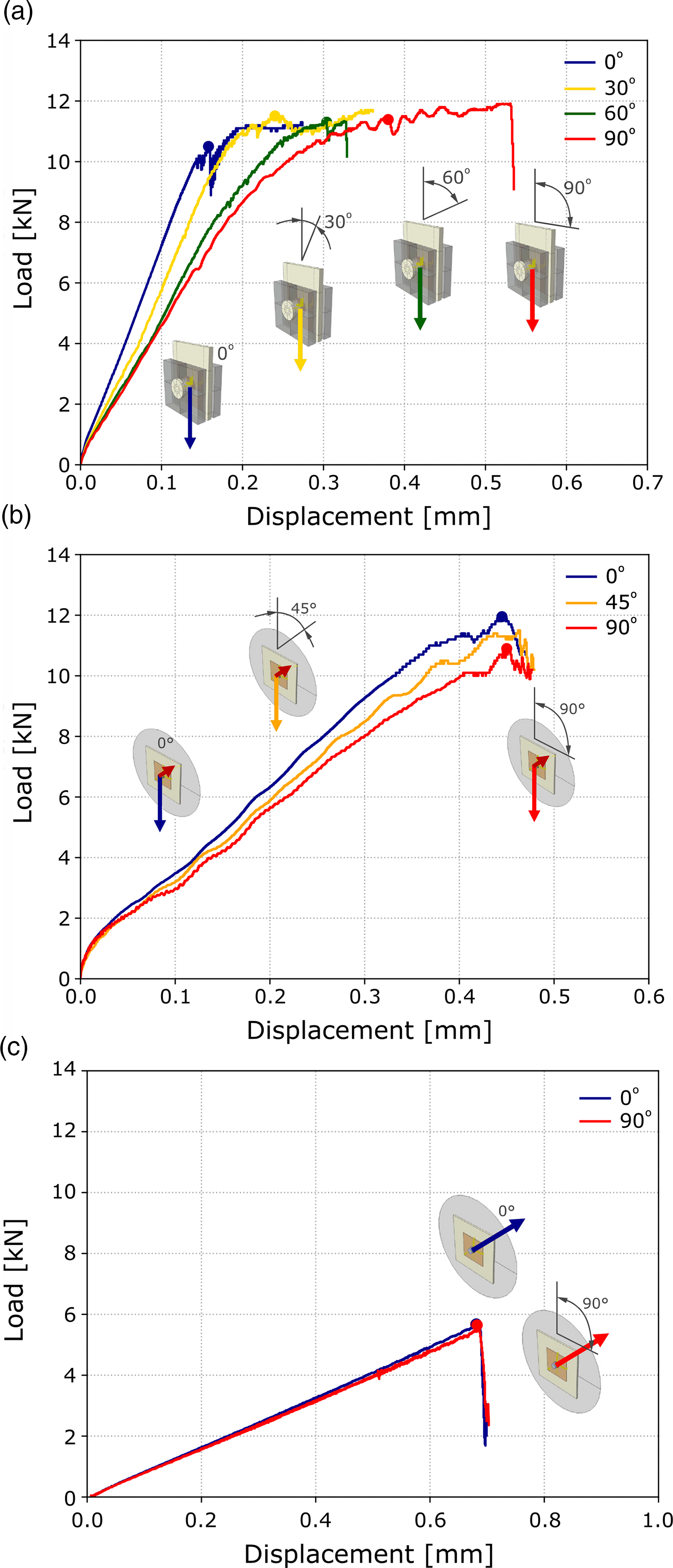
Numerical load-displacement curves for three representative load ratios. (a) η = 1.0. (b) η = 0.8. (c) η = 0.0.

The failure loads under pull-through conditions are shown to be lower than those under bearing loading due to the nature of the through-the-thickness delamination-driven failure that occurs when the bolt is loaded out-of-plane, as supported by experimental evidence (Ref. 17). Additionally, the peak loads under longitudinal bearing are found to be significantly higher than those under transversal bearing, showcasing the impact of bearing load alignment on the laminate’s stiffness and strength. The only exception can be seen in the pure bearing cases, where the highest peak load appears to be achieved when the in-plane load is applied perpendicular to the primary fiber direction. The peak load is delayed in the transversal bearing case by a large non-linear behavior, which was not captured in the longitudinal one due to numerical errors that led to early stop of the simulation. Alternatively, this may be attributed to localized damage accumulation in the contact area between the bolt and its housing in the longitudinal bearing case, leading to premature fiber breakage and specimen failure. A more comprehensive analysis should include the full load-displacement curves for further evaluation. The simulations also predicted an increase in bearing loads in the η = 0.8 case compared to the η = 1.0 case, likely as a consequence of the indirect rise in clamping force caused by the introduction of pull-through loading. Finally, the pure pull-through cases coincide in a singular value of joint resistance given that this parameter is strictly dependent on the out-of-plane stiffness, which remains consistent as the laminate is rotated.¹ The failure modes of each longitudinal sample are illustrated in Figure SI.2.

Multiaxial failure envelope and analytical equation

The failure load predictions were used to derive the two-dimensional failure envelopes in the three main planes presented in Figure 3(a) and (b), which led to the determination of the three-dimensional ellipsoidal failure criterion. Longitudinal bearing consistently results in higher peak load values due to the resistance offered by the fibers parallel to the loading direction. When the load is applied perpendicular to the principal direction, the loss of structural integrity occurs earlier, as the compressive and shear strength of the matrix is much lower than the strength of the fibers. Figure 3(c) displays the finalized three-dimensional failure envelope, fitted with the least squares method. The ellipsoid equation that most accurately represents the numerical data is given by equation (1), where f_PT, f_LB, and f_TB represent the pull-through, longitudinal bearing, and transversal bearing loads at failure, respectively.

{(\frac{f_{T B}}{11.786})}^{2} + {(\frac{f_{P T}}{5.799})}^{2} + {(\frac{f_{L B}}{12.737})}^{2} = 1

(1)

Figure 3.

Numerically determined failure envelope of the [45/90/−45/0/0/45/0/0/−45/0]_S IM7/8552 laminate, fitted with an ellipsoidal equation using the least squares method. (a) Comparison between longitudinal and transversal bearing-pull-through planes. (b) Longitudinal-transversal bearing plane. (c) Three-dimensional numerical failure envelope.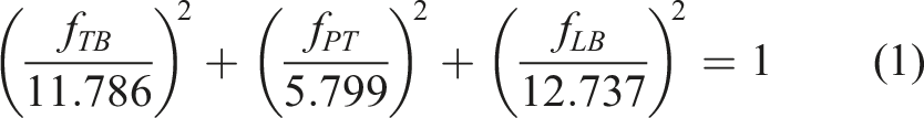

Some inaccuracies are shown to arise from the fitting method in the longitudinal and transversal bearing planes. These deviations may be corrected by using other spatial interpolation methods, such as triangulation,³¹ bicubic splines,³² Clough-Tocher splines,³³ Radial Basis Functions,^34,35 or by simply increasing the number of data points. Improving ellipsoidal fit accuracy will likely also improve failure predictions, provided that the dataset is obtained with experimentally validated and reliable numerical models. The determination of the analytical fitting equation that best describes the 3D ellipsoidal failure envelope enables its application as a failure criterion in various bolted structures, as will be discussed in the following sections.

Single-lap multi-bolt models

In this section, the high-fidelity single-lap multi-bolt models and their equivalent simplified representations are introduced. The 3D ellipsoidal failure criterion determined above is used alongside the simplified models to achieve three main objectives: (i) accurately predict the first-drop laminate-level failure in simplified models, (ii) reliably estimate the load ratio of each bolt at the moment of initial failure, and (iii) reduce the computational cost associated with high-fidelity analyses.

First, the high-fidelity multi-bolt single-lap-shear modeling strategy and numerical results are presented. Next, the simplified connector-based models are defined and their results are compared with those of the high-fidelity models.

High-fidelity modeling

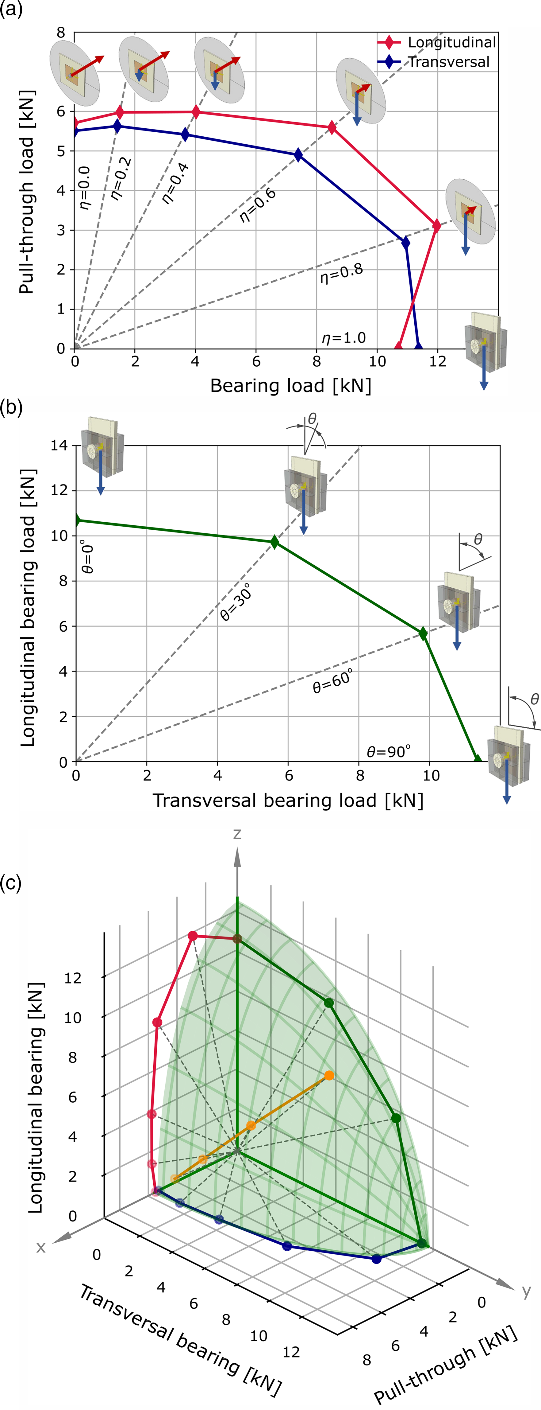
The single-lap models investigated in this study include a single-bolt case and four multi-bolt configurations whose dimensions are shown in Figure 4: the two laminates of equal layup ([45/90/−45/0/0/45/0/0/−45/0]_S) are connected with two or three bolts in tandem along the loading direction, two bolts in tandem across the width of the specimen, or by a 2 × 2 bolt pattern.

Figure 4.

Joint dimensions for different multi-bolt configurations, where N_W and N_L are the number of bolts along the specimen’s width and length, respectively. Both substrates are composite with a [45/90/−45/0/0/45/0/0/−45/0]_S layup.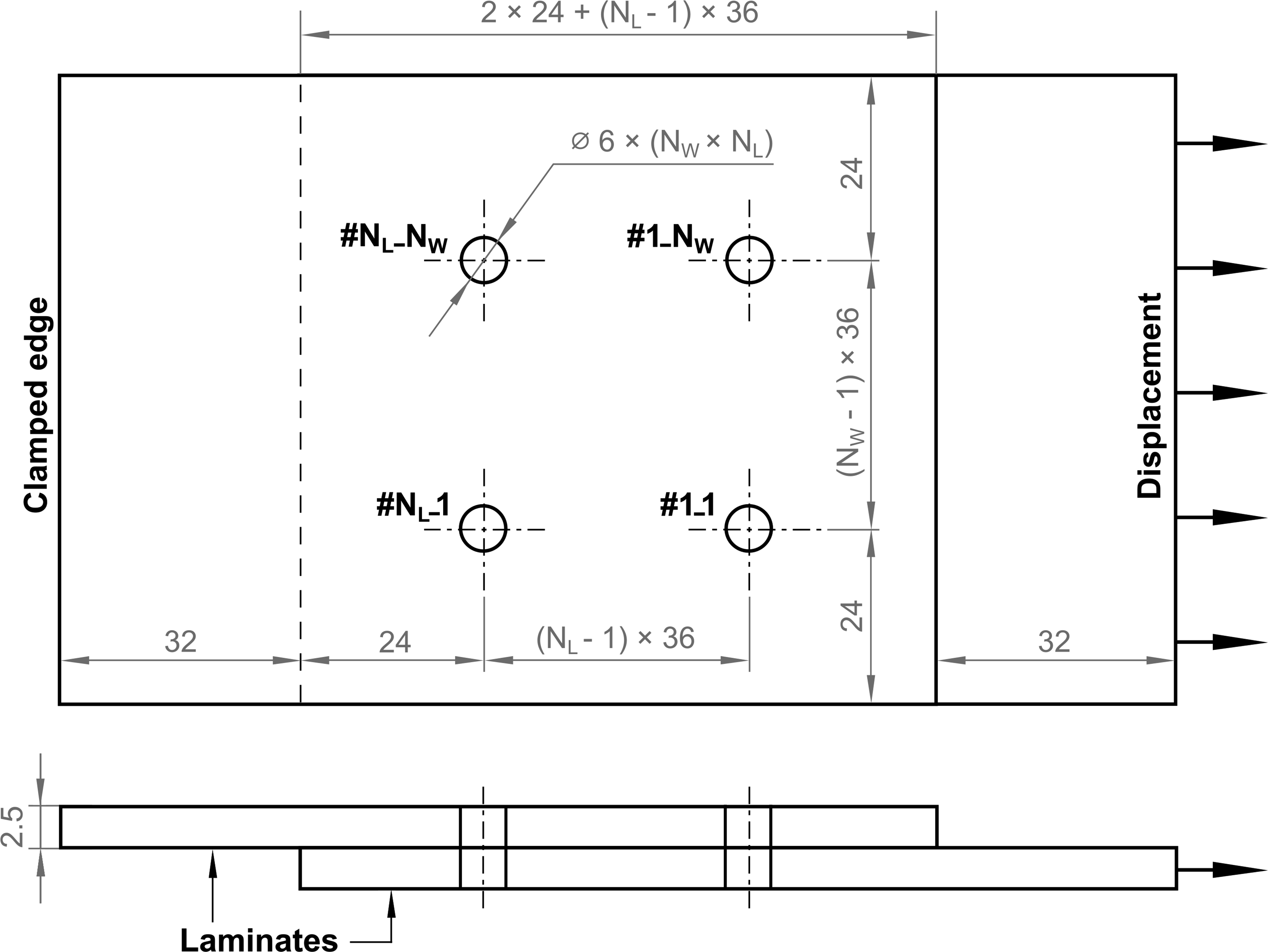

The boundary conditions applied to the multi-bolt models and all high-fidelity configurations are shown in Figure 5. The outer edge of the lower laminate is clamped, while the opposite side of the upper laminate is constrained in the y and z directions. A displacement controlled by a smooth velocity was applied along the constrained edge parallel to the joint. Given the direction of the applied displacement, and since any potential out-of-plane loading can only be attributed to secondary bending, damage in the specimen is expected to be highly localized with large load ratios, indicating a higher prevalence of longitudinal bearing loads. To reduce computational time, the size of the inner refined damageable regions were reduced to 36 × 36 mm² per bolt, instead of using the full damageable area of the combined-loading model (50 × 50 mm²).

Figure 5.

Assembly, boundary conditions and constraints used in the high-fidelity multi-bolt simulations.

The joint configurations examined here are assumed to comply with the dimensions and the relative distances shown in Figure 4. An internally-developed Python code¹⁷ was also used here as a tool for mesh partitioning, to allow structured and aligned meshes along the fibers of each ply in a 12 × 12 mm² square centered on the bolt hole axes. In compliance with the modeling approach described in the Modeling strategy section, the damageable laminates are composed of 20 plies modeled using 0.5 × 0.5 × 0.125 mm³ linear hexahedral C3D8R (and occasional C3D6R) elements connected by 0.5 × 0.5 × 0.001 mm³ COH3D8 cohesive elements.

Tie constraints were used to connect each individual ply to its adjacent cohesive layer and to join the inner and outer laminates. Surface-to-surface contact pairs were applied between each contacting part, and contact constraints were imposed among facing regions in consecutive plies to prevent penetration after the failure of the cohesive layer. All bolts were tightened with a torque of 2.2 Nm obtained by applying a temperature differential to the washer such that a bolt stress of σ ≈ 60 MPa is reached.

Overall, the high-fidelity multi-bolt models were composed of between 238,672 and 961,144 C3D8R elements, 1408 to 5632 C3D6 elements, and 261,440 to 857,888 COH3D8 elements, requiring 14 to 36 h of computational time to reach the first load drop on a 24 2.19 GHz CPU workstation with 256 GB of physical RAM.

Failure load and load ratio predictions

The load-displacement curves for each high-fidelity configuration are presented in Figure 6. As expected, an increase in the number of bolts in length or width reduces the stress in each bolt, resulting in higher joint resistance values. Note that a slight non-linearity can be observed in the initial stages of displacement. This is likely attributed to the physical clearance of 10 µm used in the high-fidelity simulations. As displacement is applied, the fasteners come into contact with the hole edges asynchronously, leading to uneven load bearing. Consequently, the laminate experiences a gradual increase in load rather than an immediate linear response. However, a small, uniform clearance is unlikely to cause significant discrepancies in peak load and stiffness, e.g. contributing to fastener failure before the laminate is fully engaged.

Figure 6.

Numerical load–displacement curves for all high-fidelity multi-bolt joints and predicted failure modes illustrated for the 2 × 1 case. Labels are defined by the number of bolts in length × number of bolts in width (N_L × N_W).

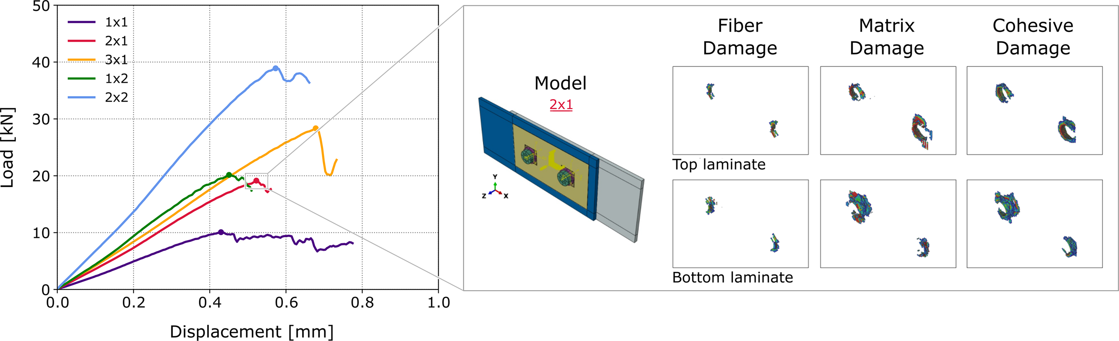
The failure modes for the 2 × 1 tandem multi-bolt configuration are also illustrated in Figure 6. For the sake of completeness, the failure modes predicted for the remaining configurations are presented in Figure SI.3. As expected, bearing loads dominate the single-lap joint configurations, as confirmed by the prevalence of localized ply-crushing around the contact area between the fastener and its housing. The bypass effect, caused by the distribution of load through the fasteners and across the composite laminate, is also identifiable in all configurations where N_L >1. By visual observation, the extent of fiber, matrix, and cohesive damage suggests an overall higher load ratio (η ≈ 0.8) for every fastener on the verge of failure, with a smaller contribution of through-the-thickness loads induced by secondary bending.

The load ratios, calculated for each fastener at the instant of failure using the Free Body Cut functionality available in Abaqus, are summarized in Table 3. The η values are found to range from approximately 0.730 to 0.814. This indicates that the visual assumption for the load ratios is reasonable and well supported by the failure mode analysis.

Table 3.

High-fidelity load ratios. The bolt references can be seen in Figure 5.

Model	Bolt	Load ratio^a
1 × 1	1_1	0.730
2 × 1	1_1	0.777
2 × 1	2_1	0.783
3 × 1	1_1	0.814
	2_1	0.785
	3_1	0.775
1 × 2	1_1	0.781
1 × 2	1_2	0.779
2 × 2	1_1	0.748
	2_1	0.755
	1_2	0.749
	2_2	0.748

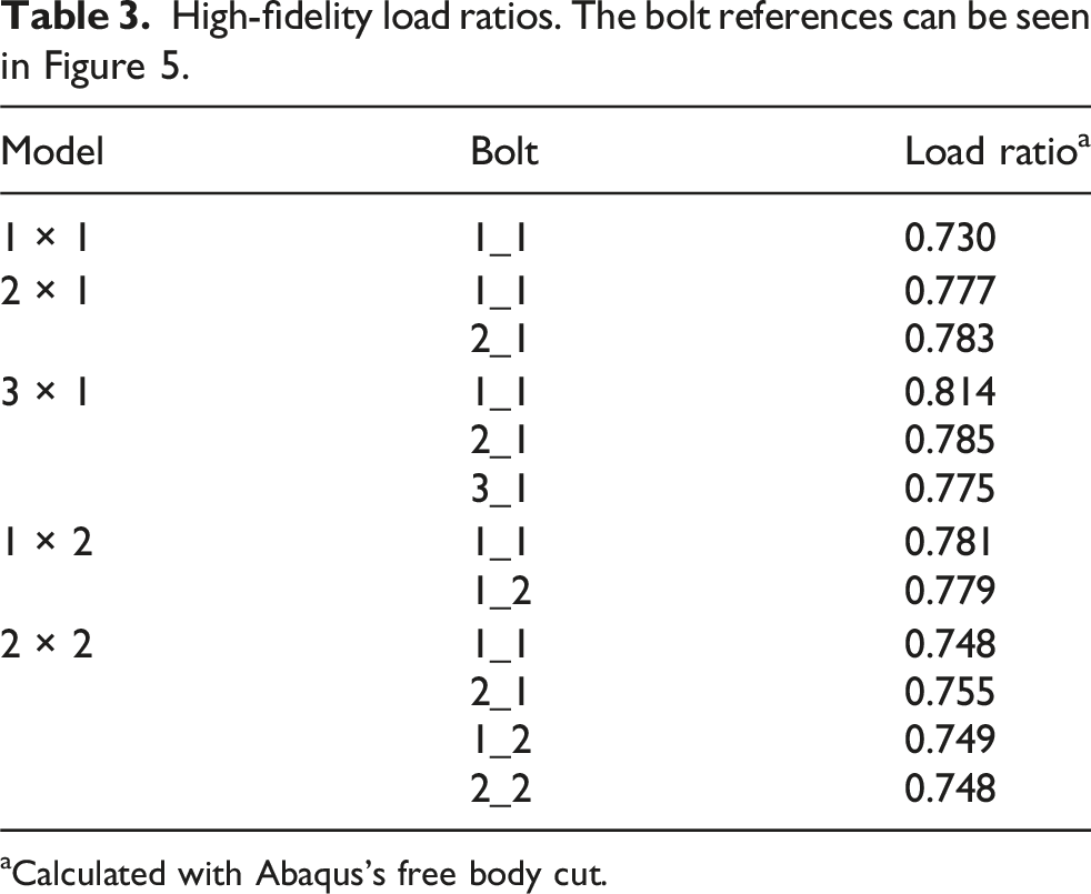
^aCalculated with Abaqus’s free body cut.

Simplified connector models

High computational expenses constitute a major disadvantage of high-fidelity numerical analyses. Despite their accuracy, the complexity of these models renders them unsuitable for large-scale structural simulations. To reduce computation time, a simplified bolt-modeling strategy is presented for the introduction of fasteners in simplified multi-bolt models. Abaqus-defined connector elements are employed here to represent bolts. The connector stiffness was calibrated to match the overall elastic response of the high-fidelity models under pure bearing and pure pull-through analyses.

The main objectives of the simplified models, used in conjunction with the analytical failure criterion derived from the ellipsoidal envelope (equation (1)), are to: (i) accurately simulate the joint stiffness for all multi-bolt structures using a single connector stiffness configuration, (ii) correctly predict the load ratios at failure in each fastener upon the application of the failure criterion, and (iii) closely estimate the first peak load, indicating first-drop laminate-level failure, while significantly reducing computational time.

Pure bearing model

The simplified pure bearing model is composed of a 36 × 43 mm² composite laminate and 2 36 × 36 × 6 mm³ steel plates. All parts are modeled with 1 × 1 mm² 4-node linear elastic shell elements with reduced integration (S4R), resulting in a total of 5903 elements. The material parameters used in the definition of the composite layup in the simplified modeling strategy correspond to the elastic properties of the IM7/8552, summarized in Table 7 (see Appendix A.4). As in the high-fidelity model, the outer edge of the composite laminate is clamped, while a 1 mm displacement, deliberately selected to exceed the maximum displacement achieved by the high-fidelity analyses, is applied to both steel blocks in the direction of the joint.

Surface-to-surface contact was defined between the overlapping section of the laminates with a “Hard” contact normal behavior. Although present in the high-fidelity model, the steel-composite penalty friction coefficient was not considered in this analysis. Instead, friction was taken into account in the connector stiffness calibration step explained below. Abaqus-defined connector elements are used to attach each steel plate to the composite laminate by the means of a circular region of influence defined as the area of the washer used in the high-fidelity models to accurately predict the clamping performance.

The effects of employing an alternative region of influence, consisting of the bolt’s cross-sectional area, were also investigated, as discussed in Section SI.4 of the supplemental material. This secondary approach was later disregarded, as the positive outcomes associated with the area for the kinematic couplings appeared to be coincidental rather than presenting substantial physical significance. Partitioning was used to enable refined, structured meshing, namely around the area of influence.

Pure pull-through model

The simplified model for the simulation of pure pull-through conditions consists of an analytical rigid shell rig with a ⌀35 mm clearance hole and a 84 × 84 mm² shell laminate modeled with 7372 S4R elements. The rig is clamped in place to avoid unwanted movement, while the composite plate is constrained at the midpoint of each edge to avoid the rotation of the specimen along the z-axis and its translation in the x- and y-directions. An out-of-plane displacement of 1 mm was applied to the free edge of the connector element along its axis.

Single-lap multi-bolt model

The simplified multi-bolt laminates are constituted by two composite laminates arranged in the aforementioned multi-bolt configurations, and modeled as planar shells simulated with 7872 to 18,248 linear elastic S4R elements (for models 1 × 1 and 2 × 2, respectively). Given the simplicity of these models, a fine mesh was adopted to maximize accuracy, as any associated increase in computational cost was expected to be negligible compared to the one of high-fidelity models. Model dimensions and boundary conditions from the high-fidelity methodology were replicated, as shown in Figure 7.

Figure 7.

Assembly, boundary conditions and constraints used in the simplified pure and multi-bolt combined-loading simulations.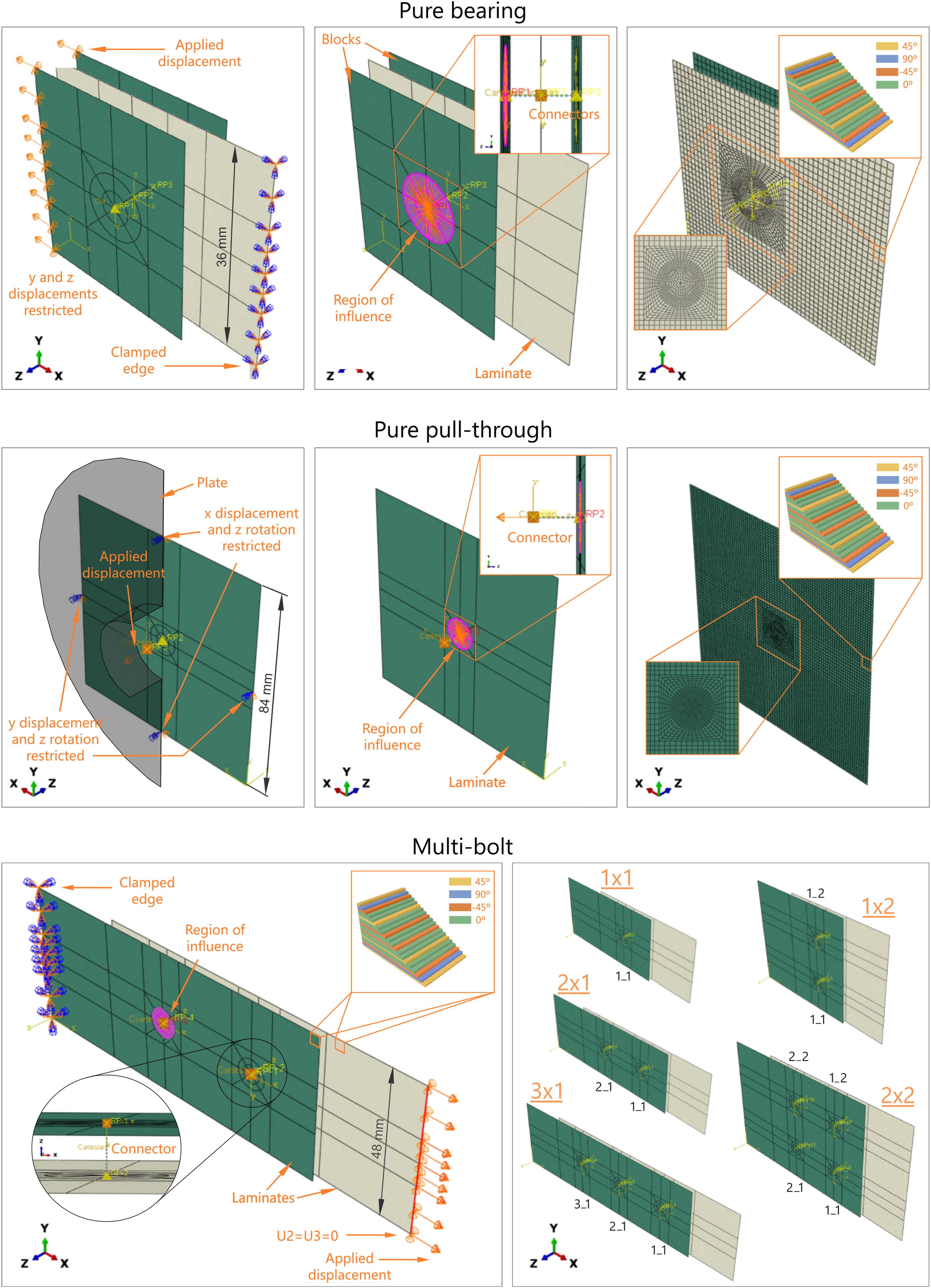

Connector stiffness calibration

Abaqus-defined cartesian connectors were selected for all simplified models. These elements allow for independent behavior exclusively along the translational degrees of freedom by measuring the positional change of the end node along the local coordinate directions.³⁶

Abaqus-defined connector elements require an a priori determination of the connector stiffness. Although this parameter can be estimated through various empirical connector flexibility equations,²¹ the most adequate formula for different laminates and joint geometries is poorly understood given the significant disparity between formulae. Therefore, to ensure the highest possible degree of accuracy, the connector stiffness was obtained through an iterative calibration procedure until the slopes of the high-fidelity simulations for pure bearing and pure pull-through were matched, as shown in Figure 8. The resulting connector stiffness values corresponding to pure bearing and pure pull-through are 49,500 N/mm and 18,500 N/mm, respectively. The markers indicate the joint resistance values taken from the intersection between the failure ellipsoid and the longitudinal bearing and pull-through axes. The resistance of the pull-through model closely aligns with the strength anchor point along the pull-through axis. In contrast, a larger difference was found between the high-fidelity and simplified pure bearing predictions, driven by inherent limitations of the ellipsoidal fitting.

Figure 8.

Stiffness comparison between high-fidelity pure pull-through and pure bearing simulations and corresponding calibration analyses with simplified pure models.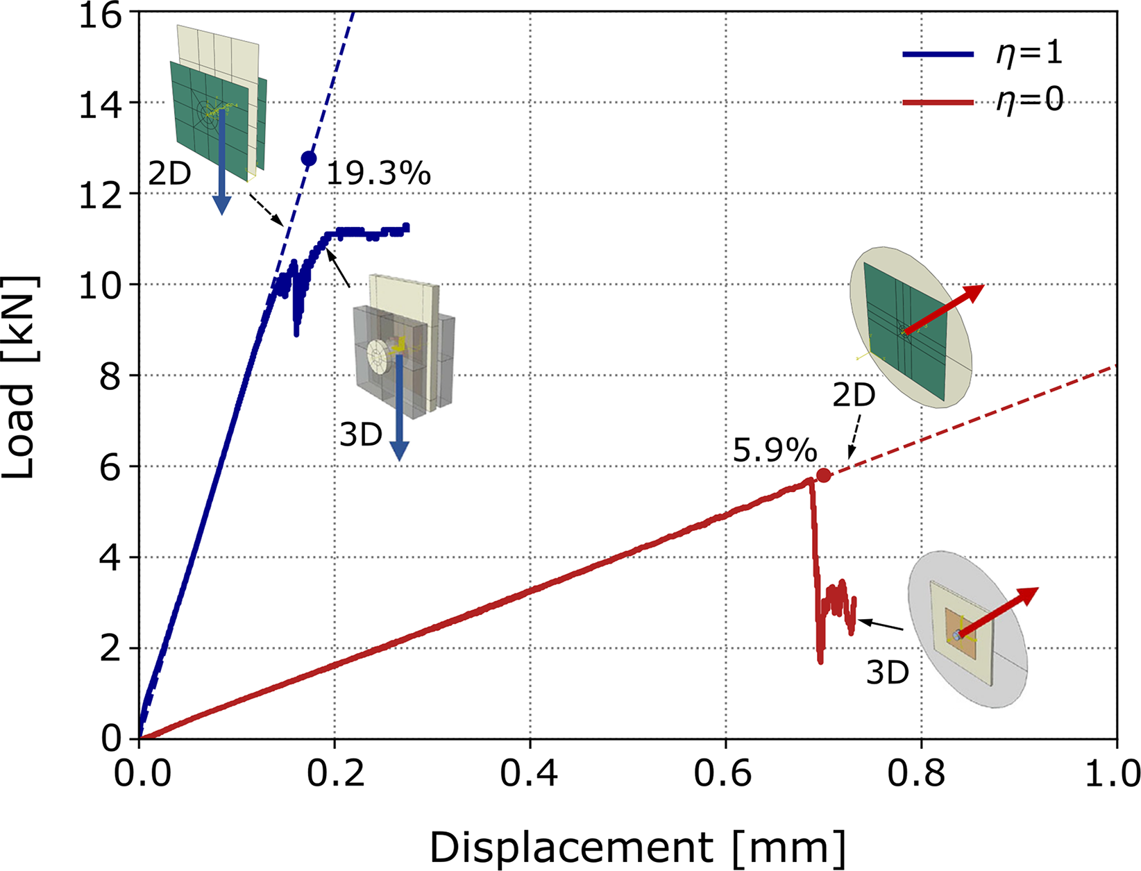

Multi-bolt simulations and post-processing methodology

The resulting stiffness values identified in the previous section were used as inputs for all the other simplified multi-bolt models. The pure bearing stiffness measure was inserted as the connector stiffness along the two bearing directions (x- and y-axes), while the pure pull-through value was selected for the connector stiffness through the laminate’s thickness. The numerical analyses were run up to a displacement of 1 mm in under 5 min using 10 2.70 GHz CPUs on a workstation with 16 GB of physical RAM. Figure 9 demonstrates that the stiffness values assigned to the connector elements accurately predict the joint stiffness across all test cases, suggesting that the simplified model remains valid without requiring significant modifications when varying the number of fasteners in a single-lap joint configuration. Despite the limitation of the connector method regarding the calibration procedure, this outcome suggests that no additional steps are necessary to support the simplified modeling strategy.

Figure 9.

Joint resistance predictions for all multi-bolt configurations using the contact area of the washer as the region of influence. The dashed lines represent the results from the simplified analyses.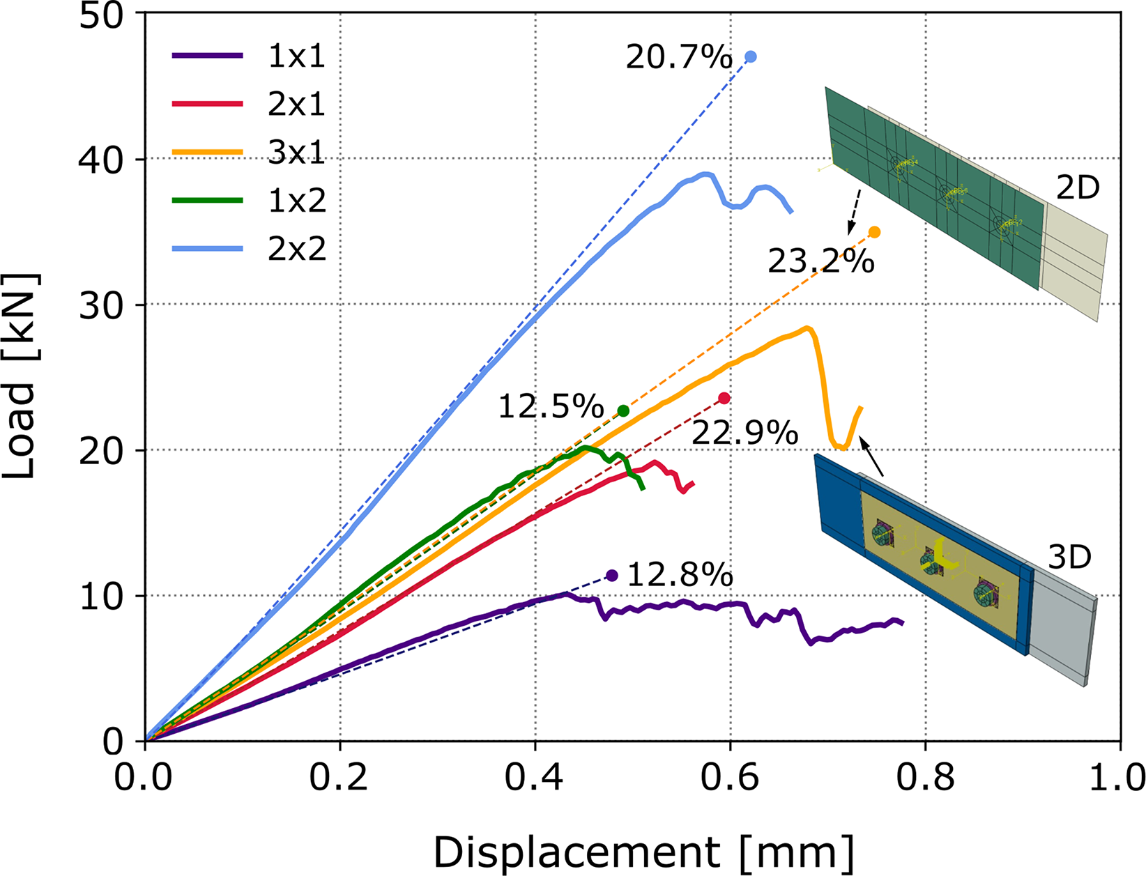

The joint strength prediction was evaluated through a post-processing methodology incorporating the analytical failure criterion. The connector forces, Cf_LB, Cf_TB, and Cf_PT, representing the bolt forces in the three main loading directions (longitudinal bearing, transversal bearing, and pull-through, respectively) throughout the simulation, were extracted for each representative fastener as a function of the joint displacement and plotted as a 3D vector alongside the ellipsoidal envelope. By extracting the bolt forces directly from Abaqus, this methodology considers the effect of non-linearity in the bolt forces, demonstrating that the bolt loading ratio varies as the joint rotates during loading. A simplified linear approximation may also be achieved by plotting a 3D vector directly connecting the origin to a force coordinate that lies outside the bounds of the failure envelope. This method would decrease post-processing time, but accuracy would be compromised as it overlooks bolt ratio variation.

Finally, the bolt loads at the moment of first-drop laminate-level failure are calculated by defining the intersection point between the non-linear connector force vector and the ellipsoidal surface, represented by a light blue marker in Figure 10. As an alternative to this post-processing method, any coordinate of the intersection point can be imported directly into Abaqus as an upper-bound failure criteria for the connector along its specified direction. Once the failure load is reached, the connector element fails, and the supported load rapidly drops to zero. Note, however, that a sudden loss of load-bearing capability is characteristic of bolt shear failure. For a more accurate simulation of bearing failure, the steep drop in resistance would be followed by a non-linear load increase until the ultimate bearing strength is reached.

Figure 10.

Intersection point between connector force curve and failure envelope. The light blue curve represents the evolution of Cf_LB, Cf_TB and Cf_PT of one of the bolts of the 1 × 1 joint as it is loaded. The intersection point between the curve and the analytical failure ellipsoid is shown as a blue dot.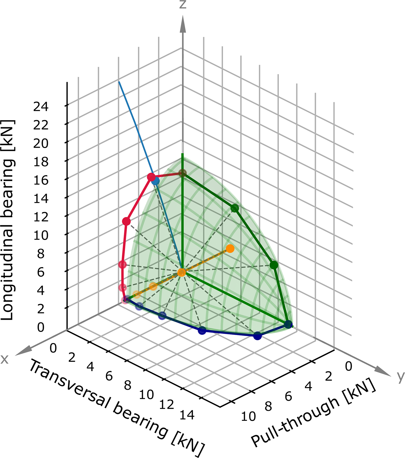

Results and discussion

Verification of the load ratios

In this work, laminate-level failure is predicted by the first load drop, which marks the onset of damage mechanisms that compromise the structural integrity and reliability of the joint. Thus, the joint resistance given by the first failed bolt (at lowest displacement) was chosen for the strength prediction. The remaining intersection values are deemed invalid as load ratio and joint resistance predictors, since these fail to consider the effect of load redistribution and the creation of different load paths upon singular bolt failure. However, it is still possible to evaluate the response of all bolts at the moment of first bolt failure, prior to any load redistribution.

The load ratios for each fastener in the high-fidelity multi-bolt configurations were measured at the first peak load and compared with the load ratios extracted from the simplified models. The η ratio in the first failed bolt is calculated directly from the intersection coordinates. Observing the ratios summarized in Table 4, it is clear that the simplified multi-bolt models are able to accurately capture the η ratio for the first failed bolt, with relative errors ranging from 1.4% to 10.8%.

Table 4.

Load ratios obtained for the first failed bolts in the high-fidelity and simplified analyses.

Model	High-fidelity	Simplified
Model	η [—]	η [—]	Error (%)
1 × 1	0.730	0.809	10.8
2 × 1	0.783	0.794	1.4
3 × 1	0.775	0.797	2.8
1 × 2	0.779	0.807	3.6
2 × 2	0.748	0.792	5.9

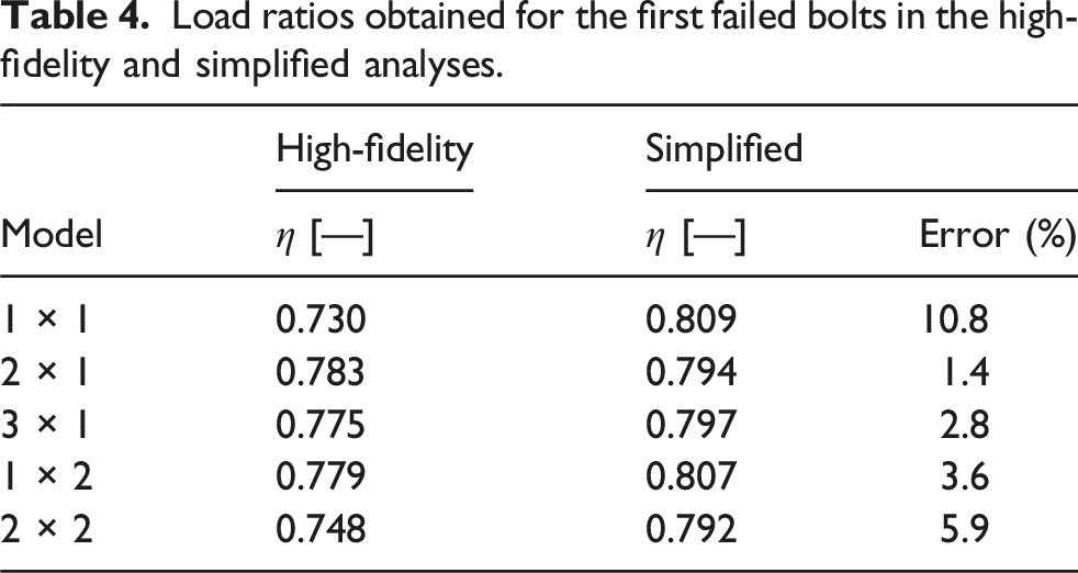
To calculate the remaining η ratios, new intersection coordinates are obtained for each bolt by interpolating the connector force curves at the point of displacement and joint resistance defined by the first failed bolt. The load ratio of the remaining bolts (shown in Table SI.5) cannot be estimated with an acceptable tolerance, with errors reaching a maximum of 24.5%. This is likely to be attributed to the underlying restrictions of the software’s definition of cartesian elements.

By default, cartesian connectors calculate the positional variation between two nodes with the same coordinate system, and only translational degrees of freedom are considered. The first failed bolt, nearest to the displaced edge, is positioned in the direct load path, and thus its behavior is most accurately predicted. The remaining bolts are underloaded along the pull-through direction as the connector elements lack the definition of rotational degrees of freedom and stiffness, meaning that moments caused by joint deformation cannot be transferred to fasteners nearing the clamped edge. In increasingly complex multi-bolt configurations, the rotational DOF limitations of cartesian elements would further affect bolt ratio and failure load predictions. However, for the cases analyzed in this work, the simplified model ratios are shown to follow a similar trend to the high-fidelity ratios, reflecting an upward progression across bolts along the length of the specimen, although the specific values differ.

Failure load predictions

The relative errors for the joint resistance values range from 12.8% to 23.2%, offering a relatively large overprediction of the joint strength, as shown in Table 5. A visual representation of the results is illustrated in Figure 9. While the prediction of overall joint strength, particularly in multi-bolt configurations, may not be optimal, it is worth emphasizing the importance of accurately determined load ratios, which are essential to avoid obtaining favorable strength values by chance. Would this analysis be repeated with different connector elements, or using a Vectorized User-Defined Element (VUEL) for the definition of the non-linear fastener behavior, the primary focus must be set on accurately assessing the correct load ratios.

Table 5.

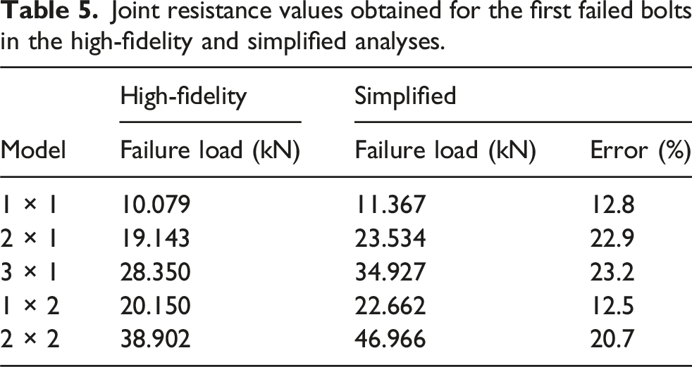
Joint resistance values obtained for the first failed bolts in the high-fidelity and simplified analyses.

Model	High-fidelity	Simplified
Model	Failure load (kN)	Failure load (kN)	Error (%)
1 × 1	10.079	11.367	12.8
2 × 1	19.143	23.534	22.9
3 × 1	28.350	34.927	23.2
1 × 2	20.150	22.662	12.5
2 × 2	38.902	46.966	20.7

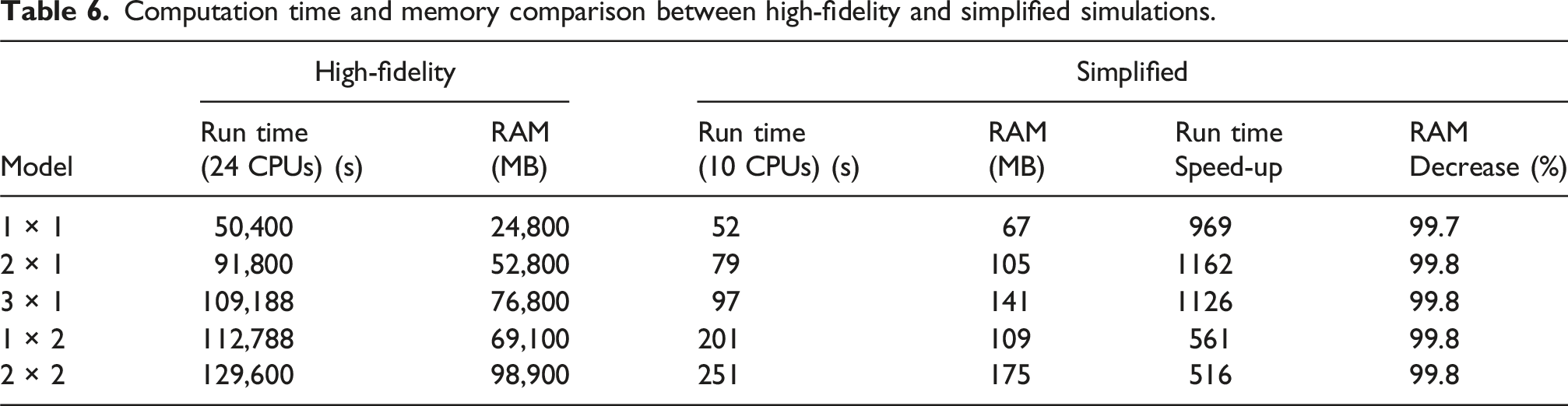
Computational time analysis

Table 6 displays the difference in computation time and memory between high-fidelity and simplified analyses. A significant reduction in run time was observed across all test cases, with the more demanding 2 × 2 case demonstrating a run time speed-up by a factor of 516. A notable decrease in RAM was also achieved in all simplified simulations.

Table 6.

Computation time and memory comparison between high-fidelity and simplified simulations.

Model	High-fidelity		Simplified
	Run time	RAM	Run time	RAM	Run time	RAM
	(24 CPUs) (s)	(MB)	(10 CPUs) (s)	(MB)	Speed-up	Decrease (%)
1 × 1	50,400	24,800	52	67	969	99.7
2 × 1	91,800	52,800	79	105	1162	99.8
3 × 1	109,188	76,800	97	141	1126	99.8
1 × 2	112,788	69,100	201	109	561	99.8
2 × 2	129,600	98,900	251	175	516	99.8

Methodology considerations

To enable the use of the proposed methodology in the failure prediction of composite structures employing a large number of fasteners, some methodological considerations and limitations must be addressed.

For the purposes of this work, a strictly numerical methodology is proposed to evaluate the behavior of composite joints. Based on the results obtained in Ref. 17 and summarized in Appendix A.4, the high-fidelity combined-loading model, validated alongside experimental testing, is trusted to accurately capture the performance of the material under the bearing/pull-through loading ratios under evaluation. However, the importance of experimental validation must not be overlooked, especially given that prior research has examined only one material and layup.¹⁷ Since relying solely on numerical calibration may lead to inaccuracies or unrealistic outcomes due to the misrepresentation of real mechanical phenomena, experimental validation will be necessary in future studies.

Post-failure behavior was not considered in this work due to the increased computational expenses and difficulty stabilizing the simulation to obtain the full load-displacement curves. First load drop analysis provides sufficient information to predict the onset of damage in the joint, which is the main focus of this work. However, the methodology may also be adapted to obtain a failure envelope including post-failure performance, either experimentally or numerically, provided that the chosen models can reach and accurately predict the second load drop. The main limitation of an experimentally-determined envelope would be the lack of means to evaluate the bolt loads necessary for the bolt ratio calculation, crucial to assess the validity of the connector elements. For this reason, an integrated experimental-numerical approach is suggested.

It must be noted that the experimental campaign in Ref. 17 was performed on only one type of bolt, torque, layup, ply thickness, and in standard temperature and pressure conditions. Altering any of these parameters has an impact on joint performance. Depending on the bolt preload, for example, the joint’s bearing performance may either increase, if said preload provides effective load distribution through friction, or decrease when it becomes excessive, inducing elevated local stresses.^12,37,38 This topic was explored further in Appendix B. Environmental effects, such as temperature^39–41 and moisture,^42,43 are also shown to impact joint performance. However, the numerical models used in this work do not contemplate these cases. To study the behavior of composite joints under environmental effects, the in-service conditions must be introduced in the numerical models and validated alongside experimental campaigns. The failure envelope is also significantly impacted by the material property definition, namely the compressive and frictional parameters, as discussed in Appendix A. These properties must be carefully determined alongside experiments to ensure that the models reflect real-world behavior.

The main limitation of the simplified modeling strategy coupled with numerical failure criteria is the overprediction of the joint failure loads, likely due to a combination of ellipsoid fitting inaccuracies and connector elements that do not fully reflect the behavior of a real fastener. A sensitivity analysis was performed in Ref. 44 to assess how these deviations affect the slope of the load-displacement curve, the failure load predicted by the simplified joint models, and the bolt load ratio of the first failed bolt. The slope of the joint load-displacement curve is highly dependent on the stiffness of the connector element and the Young’s modulus in the longitudinal direction ( $C_{f_{L B}}$ and E₁), both of which govern the initial stiffness of the system. The bolt load ratio η was shown to be primarily affected by the longitudinal Young’s modulus and by the connector stiffness in the pull-through direction. The failure load is mainly driven by the ellipsoid radii $r_{f_{L B}}$ and $r_{f_{P T}}$ .

Conclusions

High-fidelity damage simulations, utilizing a previously experimentally validated modeling approach, were conducted to replicate pure bearing,²⁵ pure pull-through,²⁶ and combined pull-through and bearing loading tests.¹⁷ These simulations enabled the first time determination of the three-dimensional failure envelope of a directional carbon-fiber-reinforced composite joint, which was obtained through an ellipsoidal fitting of the numerically obtained data. This envelope can be used in simplified directional joint models as a predictive tool for first-bolt failure.

Five multi-bolt single-lap shear joints were simulated using two distinct approaches. The first was a non-linear high-fidelity method that employed three-dimensional elements to model the joint components, including bolts, washers, and laminates. This approach featured a ply-level representation of the laminate, capturing both intralaminar and interlaminar damage onset and propagation. The second approach was a linear-elastic, low-fidelity strategy where the laminates were modeled using shell elements, and bolts and washers were represented using connector elements. The stiffness of the connector elements was calibrated by matching the stiffness of the high- and low fidelity pure bearing and pure pull-though simulations. After stiffness calibration of the connector elements, the low-fidelity models successfully replicated the stiffness across all multi-bolt single-lap shear configurations (errors below 5.8%).

The connector forces and corresponding loading ratios were calculated for both the high-fidelity and low-fidelity simulations, demonstrating excellent agreement at the point of failure (below 10.8%). In the low-fidelity simulations, failure was modeled by intersecting the connector forces with the failure ellipsoid. A satisfactory match in failure load was obtained (average of 18.4%) with a decrease in simulation time of more than 500 times. Further improvements on the failure load estimation and supporting the results with experimental validation would enhance the accuracy of the proposed method and ensure its suitability for the stress analysis of large composite structures.

Supplemental material

Supplemental Material - Integrating laminate-level bolted joint failure envelope data into connector-based finite element models for composite joint stiffness and failure prediction

Supplemental Material for Integrating laminate-level bolted joint failure envelope data into connector-based finite element models for composite joint stiffness and failure prediction by A. Volpi, F. Danzi, F. Otero, G. Catalanotti and C. Furtado in Journal of Composite Materials.

Footnotes

Acknowledgements

The authors are thankful to Rodrigo Tavares and Luís Pereira for their help developing part of the source code used in this work and for their constructive feedback and insightful suggestions.

ORCID iDs

Anna Volpi

Fermin Otero

Giuseppe Catalanotti

Carolina Furtado

Funding

The authors disclosed receipt of the following financial support for the research, authorship, and/or publication of this article: C.F. acknowledges the financial support by national funds through the FCT/MCTES, under the project 2023.15692.PEX – JOIN3D - JOInt eNergy absorption with Double-Double Design, with DOI .

Declaration of conflicting interests

The authors declared no potential conflicts of interest with respect to the research, authorship, and/or publication of this article.

Data Availability Statement

The data that support the findings of this study are available from the corresponding author upon reasonable request.*

Supplemental material

Supplemental material for this article is available online.

Note

Appendix

References

Gray

McCarthy

. A global bolted joint model for finite element analysis of load distributions in multi-bolt composite joints. Compos B Eng 2010; 41(4): 317–325.

Askri

Bois

Wargnier

, et al. A reduced fastener model using multi-connected rigid surfaces for the prediction of both local stress field and load distribution between fasteners. Finite Elem Anal Des 2016; 110: 32–42.

Kapidžić

Nilsson

Ansell

. Finite element modeling of mechanically fastened composite-aluminum joints in aircraft structures. Compos Struct 2014; 109: 198–210.

Kim

Yoon

J-C

Kang

B-S

. Finite element analysis and modeling of structure with bolted joints. Appl Math Model 2007; 31(5): 895–911.

McCarthy

Padhi

. A simple method for determining the effects of bolt–hole clearance on load distribution in single-column multi-bolt composite joints. Compos Struct 2006; 73(1): 78–87.

Verwaerde

Guidault

P-A

Boucard

P-A

. A nonlinear finite element connector for the simulation of bolted assemblies. Comput Mech 2020; 65: 1531–1548.

Omran

Nguyen

V-D

Jaffal

, et al. Development of a connector element for multi-material bolted-joint under tensile loading. Mech Adv Mater Struct 2019; 26(21): 1796–1807.

Liu

Yao

Zhao

, et al. An improved 2d finite element model for bolt load distribution analysis of composite multi-bolt single-lap joints. Compos Struct 2020; 253: 112770.

Verwaerde

Guidault

P-A

Boucard

P-A

. A non-linear finite element connector model with friction and plasticity for the simulation of bolted assemblies. Finite Elem Anal Des 2021; 195: 103586.

10.

Camanho

Fink

Obst

, et al. Hybrid titanium–CFRP laminates for high-performance bolted joints. Compos Appl Sci Manuf 2009; 40(12): 1826–1837.

11.

Liu

Xin

, et al. Progressive damage analysis of pfrp double-lap bolted joints using explicit finite element method. Compos Struct 2016; 152: 860–869.

12.

Zhuang

Arteiro

Furtado

, et al. Mesoscale modelling of damage in single-and double-shear composite bolted joints. Compos Struct 2019; 226: 111210.

13.

Cao

Zhi

Zuo

, et al. Mesoscale modelling of progressive damage and failure in single-lap and double-lap thin-ply laminated composite bolted joints. Compos Struct 2023; 316: 117046.

14.

Wang

Qin

Mekala

, et al. Three-dimensional progressive damage and failure analysis of double-lap composite bolted joints under quasi-static tensile loading. Compos Struct 2022; 285: 115227.

15.

Kelly

Hallström

. Strength and failure mechanisms of composite laminates subject to localised transverse loading. Compos Struct 2005; 69(3): 301–314.

16.

Catalanotti

Camanho

Ghys

, et al. Experimental and numerical study of fastener pull-through failure in GFRP laminates. Compos Struct 2011; 94(1): 239–245.

17.

Furtado

Pinto

Volpi

, et al. Combined bearing/pull-through failure envelope of composite joints: experimental setup and numerical validation. Compos Appl Sci Manuf 2023; 175: 107754.

18.

Tanlak

Sonmez

Talay

. Detailed and simplified models of bolted joints under impact loading. J Strain Anal Eng Des 2011; 46(3): 213–225.

19.

Sharos

McCarthy

. Novel finite element for near real-time design decisions in multi-fastener composite bolted joints under various loading rates. Compos Struct 2020; 240: 112005.

20.

Huth

. Influence of fastener flexibility on load transfer and fatigue life predictions for multirow bolted and riveted joints. Technical Report, 1984.

21.

Eremin

Bolshikh

Koroliskii

, et al. Methods for flexibility determination of bolted joints: empirical formula review. J Phys: Conf Ser 2021; 1925: 012058.

22.

Chandregowda

Reddy

GRC

. Evaluation of fastener stiffness modelling methods for aircraft structural joints. AIP Conf Proc 2018; 1943: 020001.

23.

Gunbring

Prediction and modelling of fastener flexibility using FE. Dissertation, Institutionen för ekonomisk och industriell utveckling, 2008. https://urn.kb.se/resolve?urn=urn:nbn:se:liu:diva-11428.

24.

McCarthy

Lawlor

, et al. Three-dimensional finite element analysis of single-bolt, single-lap composite bolted joints: part I—model development and validation. Compos Struct 2005; 71(2): 140–158.

25.

ASTM D5961/D5961 M - 17 . Standard test method for bearing response of polymer matrix composite laminates.

26.

ASTM D7332/D7332 M - 07 . Standard test method for measuring the fastener pull-through resistance of a fiber-reinforced polymer matrix composite.

27.

Camanho

Bessa

Catalanotti

, et al. Modeling the inelastic deformation and fracture of polymer composites–Part II: smeared crack model. Mech Mater 2013; 59: 36–49.

28.

Turon

Camanho

Costa

, et al. A damage model for the simulation of delamination in advanced composites under variable-mode loading. Mech Mater 2006; 38(11): 1072–1089.

29.

Turon

Davila

Camanho

, et al. An engineering solution for mesh size effects in the simulation of delamination using cohesive zone models. Eng Fract Mech 2007; 74(10): 1665–1682.

30.

Alfano

Sacco

. Combining interface damage and friction in a cohesive-zone model. Int J Numer Methods Eng 2006; 68(5): 542–582.

31.

Cazals

Giesen

. Delaunay triangulation based surface reconstruction. In: Effective computational geometry for curves and surfaces. Springer, 2006, pp. 231–276.

32.

Kineri

Wang

Lin

, et al. B-spline surface fitting by iterative geometric interpolation/approximation algorithms. Comput Aided Des 2012; 44(7): 697–708.

33.

Kosinka

Cashman

. Watertight conversion of trimmed cad surfaces to clough–tocher splines. Comput Aided Geomet Des 2015; 37: 25–41.

34.

Zhang

Cao

Zhang

, et al. A comparative study of different radial basis function interpolation algorithms in the reconstruction and path planning of γ radiation fields. Nucl Eng Technol 2024; 56(7): 2806–2820.

35.

Hong

Peng

. A combined radial basis function and adaptive sequential sampling method for structural reliability analysis. Appl Math Model 2021; 90: 375–393.

36.

Smith

. ABAQUS/standard user’s manual, version 6.6. Dassault Systèmes Simulia Corp, 2006.

37.

Sayman

Siyahkoc

Sen

, et al. Experimental determination of bearing strength in fiber reinforced laminated composite bolted joints under preload. J Reinforc Plast Compos 2007; 26(10): 1051–1063.

38.

Zhang

Zou

, et al. Effect of secondary bending and bolt load on damage and strength of composite single-lap interference-fit bolted structures. J Compos Mater 2019; 53(28-30): 4385–4398.

39.

Yang

, et al. An experimental investigation on bearing behavior and failure mechanism of bolted composite interference-fit joints under thermal effects. Eng Fail Anal 2022; 131: 105830.

40.

Zhang

Zhou

Pan

, et al. Comparison on failure behavior of three-dimensional woven carbon/carbon composites joints subjected to out-of-plane loading at room and high temperature. Compos Commun 2021; 23: 100567.

41.

Seyednourani

Akgun

Ulus

, et al. Impact damage and low temperature effects on carbon fiber/epoxy joints: a comparative study of hybrid bolted/bonded and bolted configurations with cross-ply and angle-ply laminates. Compos Appl Sci Manuf 2025; 190: 108677.

42.

Jin

Xuan

, et al. Influence of cyclical hygrothermal aging on mechanical response and structural durability of composite bolted interference-fit joints. Thin-Walled Struct 2022; 173: 108997.

43.

Karimi

Ahmadi

Klenin

, et al. An experimental investigation on the influence of environmental ageing on strength and fatigue behavior of different single lap joints. Compos Struct 2023; 322: 117423.

44.

Santos

. High- and low-fidelity damage models for composite joints. Dissertação de mestrado, Faculdade de Engenharia da Universidade do Porto, Porto, Portugal, 2025. URL: https://hdl.handle.net/10216/168691

45.

Falcó

Ávila

Tijs

, et al. Modelling and simulation methodology for unidirectional composite laminates in a virtual test lab framework. Compos Struct 2018; 190: 137–159.

46.

Bažant

. Crack band theory for fracture of concrete. Mater Construcción 1983; 16(3): 155–177.

47.

Zhuang

Chen

Arteiro

, et al. Mesoscale modelling of damage in half-hole pin bearing composite laminate specimens. Compos Struct 2019; 214: 191–213.

48.

McCarthy

Stanley

, et al. Experiences with modeling friction in composite bolted joints. J Compos Mater 2005; 39(21): 1881–1908.

49.

Catalanotti

Furtado

Scalici

, et al. The effect of through-thickness compressive stress on mode ii interlaminar fracture toughness. Compos Struct 2017; 182: 153–163.

50.

Camanho

Lambert

. A design methodology for mechanically fastened joints in laminated composite materials. Compos Sci Technol 2006; 66(15): 3004–3020.

51.

Camanho

Maimí

Dávila

. Prediction of size effects in notched laminates using continuum damage mechanics. Compos Sci Technol 2007; 67(13): 2715–2727.

52.

Raimondo

Doesburg

Bisagni

. Numerical study of quasi-static and fatigue delamination growth in a post-buckled composite stiffened panel. Compos B Eng 2020; 182: 107589.

53.

Arteiro

Catalanotti

Melro

, et al. Micro-mechanical analysis of the in situ effect in polymer composite laminates. Compos Struct 2014; 116: 827–840.

54.

Arteiro

Catalanotti

Melro

, et al. Micro-mechanical analysis of the effect of ply thickness on the transverse compressive strength of polymer composites. Compos Appl Sci Manuf 2015; 79: 127–137.

55.

Bessa

. Meso-mechanical model of the structural integrity of advanced composite laminates. Master’s Thesis, Universidade do Porto, 2010.

56.

Furtado

Catalanotti

Arteiro

, et al. Simulation of failure in laminated polymer composites: building-block validation. Compos Struct 2019; 226: 111168.

57.

Catalanotti

Xavier

Camanho

. Measurement of the compressive crack resistance curve of composites using the size effect law. Applied Science and Manufacturing 2014; 56: 300–307.

58.

Erçin

. Stress gradient effects in laminated composites. PhD Thesis, Faculdade de Engenharia, Universidade do Porto, 2013.

59.

Arteiro

. Structural mechanics of thin-ply laminated composites. PhD Thesis, Universidade do Porto, 2016.

60.

Koerber

Camanho

. High strain rate characterisation of unidirectional carbon-epoxy IM7-8552 in longitudinal compression. Compos Appl Sci Manuf 2011; 42(5): 462–470.

61.

Catalanotti

Camanho

Marques

. Three-dimensional failure criteria for fiber-reinforced laminates. Compos Struct 2013; 95: 63–79.

62.

Vogler

Rolfes

Camanho

. Modeling the inelastic deformation and fracture of polymer composites – part I: plasticity model. Mech Mater 2013; 59: 50–64.

63.

Camanho

Dávila

Pinho

, et al. Prediction of in situ strengths and matrix cracking in composites under transverse tension and in-plane shear. Compos Appl Sci Manuf 2006; 37(2): 165–176.

64.

Camanho

Dávila

de Moura

. Numerical simulation of mixed-mode progressive delamination in composite materials. Compos Mater 2003; 37(16): 0021998303034505.

65.

Tavares

CML

. Fracture of advanced composite materials: experimental basis for a constitutive model. Technical report. University of Porto, 2006.

66.

Lopes

Camanho

Gürdal

, et al. Low-velocity impact damage on dispersed stacking sequence laminates. Part II: numerical simulations. Compos Sci Technol 2009; 69(7): 937–947.

Supplementary Material

Please find the following supplemental material available below.

For Open Access articles published under a Creative Commons License, all supplemental material carries the same license as the article it is associated with.

For non-Open Access articles published, all supplemental material carries a non-exclusive license, and permission requests for re-use of supplemental material or any part of supplemental material shall be sent directly to the copyright owner as specified in the copyright notice associated with the article.

0.00 MB

19.74 MB