Sage Journals: Discover world-class research

Abstract

Resin transfer molding (RTM) is a production technique for fiber reinforced polymer components (FRPCs). It allows the embedding of sensors into components that enable production and structural health monitoring. Since void content is one of the most critical quality criteria, this study investigates the capability of embedded acceleration sensors to capture relevant information during RTM monitoring. For this purpose, a local void content classification based on sensor signals was considered, employing Machine learning algorithms for data labeling and classification. The final classifier’s performance was estimated using nested Cross-Validation (nested CV) and a hold-out test set. While the mean CV-estimates exceeded values over 89% for the main measures F_1.14, F₁, Recall and Precision, the overall performance on the hold-out set decreased to F_1.14 = 79%, F₁ = 78%, Recall = 88% and Precision = 70%. Model analysis revealed that the small, imbalanced data set led to instability, and that generalization errors from labeling affected the classifier. Nonetheless, class structure was visible in the frequency domain, confirming that the sensors recorded void content information. Furthermore, the main limitations can be addressed by transitioning from laboratory-scale to series production. This study hence provides a foundation for quality control of acceleration sensor embedded FRPCs produced via RTM.

Keywords

resin transfer molding voids sensors artificial intelligence

Introduction

Fiber reinforced polymer components (FRPCs) are used in various industries, such as automotive and aviation, for their high strength-to-weight ratio^1,2. A common technique in series production is Resin transfer molding (RTM), which belongs to the Liquid composite molding processes. During RTM, polymer resin is injected under pressure into a mold containing reinforcement fibers. Subsequent to curing, components are demolded and may be further processed. To improve RTM efficiency by minimizing manufacturing defects, the influences of mold design, fiber properties and process parameters on resin flow are extensively studied. One of the most significant defects are voids, which are regions unfilled with polymer and fibers, because of their impact on various composite properties and failure mechanisms combined with their high formation probability. The distinct scales of gaps between and within fiber tows lead to a competition of viscous and capillary flow. This dual scale flow promotes air entrapment on the different scales. Micro-voids within the tows are generated when the former dominates, whereas meso-voids form between tows when the latter dominates³.

According to ⁴, dual scale flow can be modeled as

\nabla (\frac{K}{μ} \cdot \nabla p) = q (p, S) .

(1)

On the left-hand side, the continuity equation for the volume averaged flow velocity

⟨v⟩

, that is

\nabla ⟨v⟩ = 0,

(2)

is combined with Darcy’s law⁵

⟨v⟩ = - \frac{K}{μ} \cdot \nabla p,

(3)

where μ is the fluid viscosity, ∇p the pressure gradient and K the permeability tensor of the fibers. The right-hand side is a sink term that models resin flowing into the fiber tows. It is dependent on the pressure p and the fibers’ saturation S. The latter can be defined as⁶

S : = \frac{V_{w}}{V_{T}},

(4)

with V_w the volume of the liquid phase and V_T the total volume of pores in the material. Simulations based on these equations are well suited for understanding void evolution. Recently, a model combining two simulations, one for the dual scale flow and one for tow filling, was employed to predict void locations and distributions. The simulations were validated through physical RTM processes under various conditions, showing good agreement⁷.

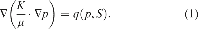
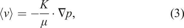
Artificial intelligence (AI) has become increasingly important to composite technologies^8,9, such that it gets also incorporated into RTM research. In ¹⁰, simulations for ultra-fast RTM were investigated by a combination of micro-, meso- and macro-scale models. To reduce computational time for repetitive meso-scale simulations, Neural networks (NNs) were trained to obtain permeability and macro-scale resin velocity from pressure gradients. Numerical validations demonstrated a good match between this approach and full simulations. Moreover, mold filling was predicted to be slower than in simulations purely based on Darcy’s law, Equation (3). In another study, an Autoencoder NN was trained as surrogate model to replace simulations¹¹. The NN mapped gray-scale images representing local permeability values and time dependent inlet pressure to simulated flow front and pressure field images. This surrogate model was physically validated with a good qualitative agreement between overall flow front shape and arrival times at specific mold coordinates. Beyond direct application in simulations, AI can be used to investigate material properties, particularly the permeability K, to improve simulation accuracy. In ¹², a Convolutional neural network (CNN) was trained to estimate permeability values from 2d images of fiber microstructures and the outputs were subsequently up-scaled to 3d. The model was tested on the virtual permeability benchmark¹³ with results well within the benchmark’s range of estimates. Moreover, resin flow can be observed and data processed to obtain permeability values, which is considered an inverse problem. For instance, a CNN was trained on simulations to parameterize regions with lower permeability¹⁴. Furthermore, the authors of ¹⁵ trained a CNN on physical RTM flow front images to estimate permeability fields. Simulations based on this CNN’s outputs outperformed simulations utilizing an averaged permeability value, as assessed by pixel-wise flow front labels and flow front shape. Other works observed resin flow and applied AI to find race-tracks¹⁶, which are unexpected resin channels often occurring at mold edges, to track the resin front¹⁷ or to optimize mold design¹⁸.

However, the application of AI to study voids is limited. In ¹⁹, the formation and transport of meso-voids was investigated. Filling of 3d-printed porous media, resembling textiles, was observed with a camera. Then, a trained U-Net model segmented the videos into flow front, bubble edge, bubble center and background. Subsequent processing algorithms were used to study different void metrics and effects on void transport. Potential quality predictions were investigated in ²⁰. First, RTM processes were simulated for molds with multiple regions of varying permeability. A part was considered defective if it had one region with less than 99.5% filling factor or a void content exceeding 1%. Ensemble models for binary classification, based on Decision trees, were trained from pressure data. It was concluded that quality prediction from pressure data is a promising approach to reduce further quality inspections.

AI-approaches are usually limited by the need for large datasets to obtain reliable model outputs. Therefore, conducting sufficiently many physical RTM processes is expensive such that only few of the aforementioned studies validate their models with real data^11,16 or rely solely on it¹⁵. These studies are primarily using pressure data because of its occurrence in equations (1) to (3). 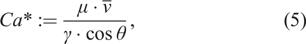Moreover, pressure data enables void content minimization by calculating the resin front velocity, for example ²¹, that appears in equations (1) to (3), and in the modified capillary number^3,22

{C a}^{*} : = \frac{μ \cdot \bar{v}}{γ \cdot \cos θ},

(5)

where

\bar{v}

is the macroscopic resin velocity, γ the resin surface tension, and θ the contact ancle between resin and fibers. Various studies show that Ca* correlates well with the saturation S. Low values relate to meso-void formation, while high values result in micro-voids. There also exists an optimal value for minimal overall void formation³. As summarized in ³, Ca* furthermore links to meso-void mobility, requiring it to exceed a critical threshold for voids to become mobile. Void mobility is also dependent on the ratio of void size to inter- or intra-tow spacing. Another common technology to monitor the resin front velocity are capacitive sensors^6,22. These usually consist of metal plates on the top and bottom of the mold cavity. Resin flow between them changes the electrical potential. Detecting this, the average resin velocity between two sensors can thus be calculated. A feedback mechanism to the inlet can then optimize resin velocity and minimize component porosity^23,24. Related studies additionally show that the measured capacitance directly correlates with the saturation, representing local residual void content between the poles.

Piezoelectric, piezoresistive, and fiber Bragg grating sensors can also detect resin fronts^25–29. Thus, using two or more sensors enables void content control. Moreover, such sensors can be embedded into components and later used for Structural health monitoring. In this context, the present study extends recent work on embedding Micro-electro-mechanical-systems (MEMS) acceleration sensors into FRPCs³⁰. The used BMA456 sensors record triaxial acceleration and temperature³¹. They have previously been employed to monitor resin front arrival during RTM^32,33, detect impacts³⁴, and show promise for lifetime prediction during fatigue testing³⁰. As elaborated, research combining void content analysis, physical sensor experiments, and AI application remains limited. This study addresses this gap by assessing local porosity around sensors based on their individual data instead of estimating the resin velocity from a network. Based on equations (1) to (5), one can expect varying resin flow dynamics, particularly when voids are transported. Thus, it is hypothesized that the BMA456s capture void content information through acceleration and temperature recordings during RTM embedding. More specifically, motivated by the use case of quality control, a local void content classification for sensor neighborhoods is investigated. Since meso-voids provided direct visual quality feedback during production, they are the primary focus. To quantify good and bad quality, a threshold for overall void content was adopted from the literature and applied to the detected porosity. Some authors consider 0.5%^35,36, other references mention values of 1%, 2% and even up to 5%^37,38. For reasons explained in the Methodology section, based on estimated void contents and data-driven considerations, a threshold of 0.5% was chosen. In this regard, the task is similar to that in ²⁰, but it is set apart by the sensor type and using only physically recorded sensor data. This latter point results from the complexity of the sensor signals. Both pressure data, as used in ^11,20, or capacitance data⁶ for RTM processes usually have an overall monotonically increasing shape that converges over time. In contrast, acceleration data displays much more complex signal curves, as exemplified in Figure 1, which makes it difficult to be simulated.

Figure 1.

Exemplary acceleration and temperature curves of a BMA456 sensor during RTM infiltration.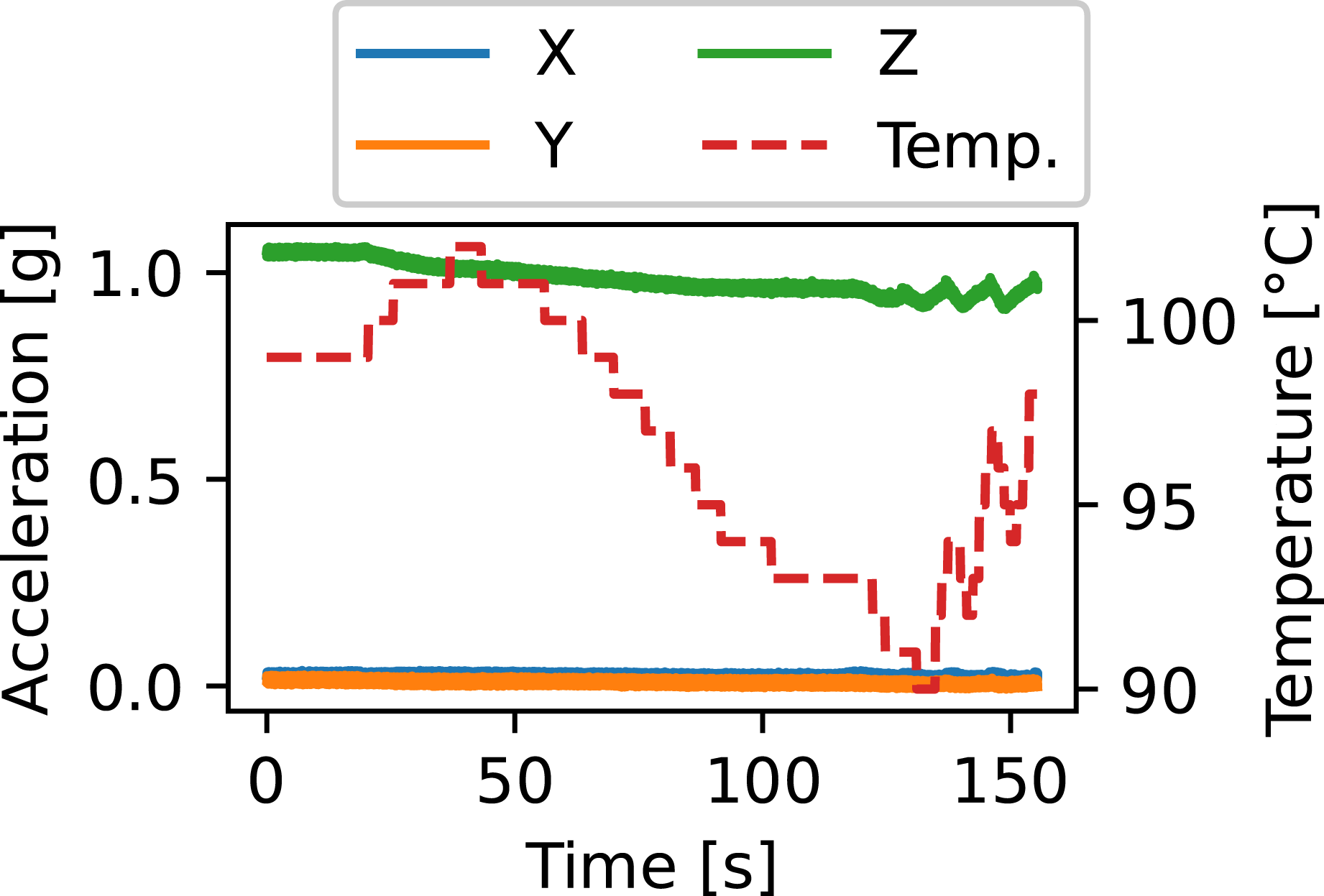

This paper is structured as follows: The subsequent methodology chapter is divided into three sections. First, the materials and the production process are described. Second, the methodology to generate void content labels for the classification task is presented. Third, the classification methodology is explained. The chapter afterwards combines results and discussions, organized into three sections. The first one contains a void analysis from SEM-micrographs. The second focuses on the labeling process. The third covers the classifiers, the data set and includes a summarizing discussion. The paper finishes with overall conclusions.

Materials and methods

Production process

Glass-fiber reinforced plates with embedded BMA456 sensors were manufactured using RTM. Detailed descriptions of the experimental setup and manufacturing process can be found in ^30,33 and sensor specifications in ³¹. However, a summary and necessary information for this study are provided below.

The German Institutes of Textile and Fiber Research Denkendorf supplied a 2/2 twill glass-fiber textile with 720g/m² areal density and 0.65mm loose thickness, made from Johns Manville StarRov® 086 600 roving. The BMA456 sensors measure 2mm × 2mm × 0.65mm and require two additional capacitors, of similar height. These components were soldered onto flexible circuit boards with approximately 287μm thickness around the sensors and capacitors, and uniform 7.5mm width. Since the circuit boards were woven directly into the textile during its production, the sensors and capacitors needed encapsulation. This was achieved with Henkel Loctite Eccobond EO 1072. The encapsulation process was restricted to add at maximum 0.05mm height. The RTM resin system consisted of Sika Biresin® CR144 resin and Biresin® CH170-3 hardening agent.

The laboratory setup consisted of a fully rigid, opaque mold, a programmable logic controller (PLC), a pressure vessel housing the resin reservoir, and a vacuum pump at the outlets. The PLC controlled mold temperature, air pressure on the resin reservoir, and inlet- and outlet-valves. Six textile layers were placed inside the approximately 3.2mm high mold cavity. The fiber-volume fraction for reference components without embedded sensors was previously determined as V_f ≈ 55.8%³⁰. 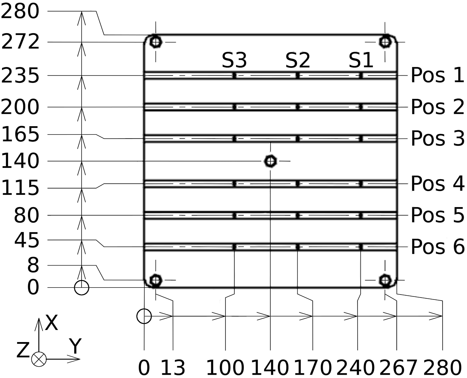Manufacturing constraints allowed only three circuit boards per cut. Consequently, layers three and four contained the circuit boards with sensor orientation toward the cavity center plane. As a result, the X- and Z-axes, representing the through-thickness direction, were mirrored between these layers. Overall, a 3 × 6 sensor grid was established. A technical drawing with dimensions and positions is shown in Figure 2. The mold inlet was centered while outlets were positioned in each corner, creating radial infiltrations with resin flow through the thickness. Manual RTM preparations followed a strict protocol covering resin-to-hardener weight ratio, degassing durations, mixture temperature before infiltration and even tube lengths. The outlet vacuum operated at −0.8bar. The PLC maintained mold temperature around 95°C and provided a monotonically but non-linearly increasing pressure up to 2bar relative pressure. This pressure was held until capacitive sensors connected to the PLC detected resin bleeding at all outlets. The PLC then executed a 36s flushing sequence with 4bar relative pressure on the resin reservoir. The outlet valves alternately closed for 7s and opened for 1s for four times. This flushing is particularly prominent in the Z-acceleration data, as can be seen in Figure 1. Parts were finally cured with closed outlet valves, maintained 4bar relative pressure and mold temperature. Remaining voids in the mold were thus compressed according to the ideal gas law. Porosity was subsequently measured as described in the next section.

Figure 2.

Technical drawing of the plate dimensions in mm. The inlet is positioned at the center and outlets are located in each corner. The coordinate system denotes the reference orientation to which the sensor signals were mapped. This figure is adapted from ³³.

This above process provided the baseline for plates with visually high quality. In particular, the flushing transported voids out of the mold and curing under increased pressure compressed remaining voids while preventing the expansion of voids resulting from the chemical reaction of resin and hardening agent. Direct visual feedback during demolding was preferable to produce components with increased porosity. Hence, focus was put on increasing meso-void content. The mold temperature, affecting resin viscosity and surface tension, or the inlet pressure could have been varied as described by equations (3) to (5). On the one hand, temperature changes would be easily detectable from the sensors’ temperature measurements. On the other hand, resin fronts of different velocities carry different momentum, hence exerting different forces on sensors upon contact, and resulting in different acceleration signatures. Moreover, such approaches would simplify the task to mappings from process parameters to void content, making sensor data obsolete. Preliminary experiments explored raising meso-void content by introducing air into the mold and without altering the baseline RTM parameters, such as connecting additional valves and airflow to the inlet tube. A stable solution was achieved by piercing one hole into the inlet tube inside the pressure vessel using a G30 cannula. Stability is hereby understood as a roughly constant air introduction into the mold per time unit, even during flushing. Each infiltration used a new cannula and inlet tube. However, slightest variations in cannula sharpness, tube hardness or resin variations, resulting from the manual preparation, influenced air bubble amount and size. A total of 19 plates with hence random overall void contents were produced. It was intended to have more of them with higher overall void content and wider respective variance, which both would be beneficial for the later classification task. Therefore, 14 plates were made with manipulated inlet tubes and five without. The former are denoted as porous, the latter as pristine. This nomenclature does not imply that porous plates had only high void content, nor that pristine plates were completely void-free due to natural causes for void generation. In total, 19 × 18 = 342 sensors were embedded. 19 failed to record their RTM processes, nine from pristine and 10 from porous infiltrations. This happened due to improper handling of the circuit boards, which were either damaged or shortcut at the mold seals. Therefore, data from 323 sensors remained available.

The BMA456 sensors measure triaxial acceleration in units of gravity and temperature with a resolution of 1°C. The circuit boards were each connected to one Arduino microcontroller. Up to three Arduinos could be connected to a measurement laptop running custom LabVIEW software. The sensors were configured to record at 1600Hz with an acceleration measurement range of ±2g. The infiltration recordings were synchronized to process starts and ends via an interface between the Arduinos and the PLC.

Void content labels from images

To preserve the plates as samples for eventual further material experiments, a non-destructive approach for local void content measurements was required. In this sense, methods such as CT-scans, optical microscope, or Scanning electron microscope (SEM) micrographs were considered destructive because they require cutting the plates into smaller analysis samples. Such methods also require special equipment and are time-intensive for over 300 samples. It is emphasized that the purpose was not to achieve exact porosity measurements but rather approximate estimates to provide good and bad labels for the classification algorithm. As mentioned above, the production was focused on meso-voids. Air bubbles introduced through the punctured inlet tube were assumed to most likely stay meso-voids because it is difficult for them to move from the relatively large inter-tow spaces into dense tows³⁹. Additionally, micro-voids transported within tows were assumed not to interact with sensors. Therefore, a photo box with image processing pipeline was set up for a simple and fast meso-porosity evaluation. This approach enabled measurements immediately after demolding and without further material processing. For calibration and validation, CT-scans for nine material samples were conducted during early production. Moreover, sensors locally influenced the fiber architecture, for example by creating inter-tow channels and compacting fiber tows. Thus, an additional SEM-analysis was carried out with four CT-samples to investigate meso- and micro-void presence in sensor neighborhoods. The remainder of this section focuses on the development of the void content measurement. The analysis of meso-and micro-voids through SEM-micrographs is presented in the first section of Results and discussions.

The self-built photo box consisted of a light pad, a Panasonic DC-TZ91 camera, an aluminum rack and a blackout curtain. The light pad was set to a warm white light color at full intensity. The camera was placed above it and set to 4K-mode, a 1 : 1 aspect ratio and automatic macro-focus. Furthermore, the ISO sensitivity, aperture and shutter speed were manually adjusted once to the lighting conditions, which remained consistent due to the blackout curtain that covered the entire photo box. Material embedded sensors could be centered and aligned under the camera thanks to visual clues given by the camera’s cross-hairs and thirds grid. Using a stencil, the distance between camera lens and plates was calibrated to produce pictures of side length 35mm × 35mm. This size was camera dependent, corresponding to the smallest distance between the camera lens and an object that the camera software allows. The image size of 3888px × 3888px provided a resolution of approximately 81μm²/px or 9μm pixel side length, denoted as μm/px. This value is similar to ⁴⁰. Moreover, void edges get blurred through material on top. This led to measurement uncertainty, dependent on the position on the material Z-axis, which was not quantified for this work. In previous work³⁰, using the exact same mold, fibers and resin system, the mean fiber diameter was measured at 16μm. Moreover, a Wald distribution was fitted to the nearest neighbor distances of a tow’s fibers with a mean of 0.68μm and a scale of 1.4μm. Therefore, it was assumed that the camera would not detect micro-voids. Their detectability is further discussed in the SEM-micrograph analysis section. To diminish void blurring effects to some extent, each of the 342 embedded sensors was photographed twice, one view from the top and one from the bottom, by flipping the plates over. These images were combined in the processing pipeline to provide area-based void content estimates. Although volume void content can be estimated from 2d images, accuracy may suffer due to high dissimilarities and limited local views³. Assumptions such as ellipsoidal void shape that can be extrapolated from the cross-sections through maintained aspect ratios and dedicated image filtering schemes⁴¹ are also needed. The camera image in Figure 3 demonstrates that the ellipsoid assumption does not hold in the present case. Therefore, this work’s void content estimation forewent such assumptions and instead prioritized ease of implementation and fast image processing by computing area-based porosity.

Figure 3.

The shown sample has a volume void content of approximately 0.65%. Top: 35mm × 35mm photo box picture, whereby the blue-dotted and red-dashed lines indicate the SEM-micrographs; Bottom: The segmentation resulting from ilastik’s Pixel Classification, foreground voids in cyan, background voids in green.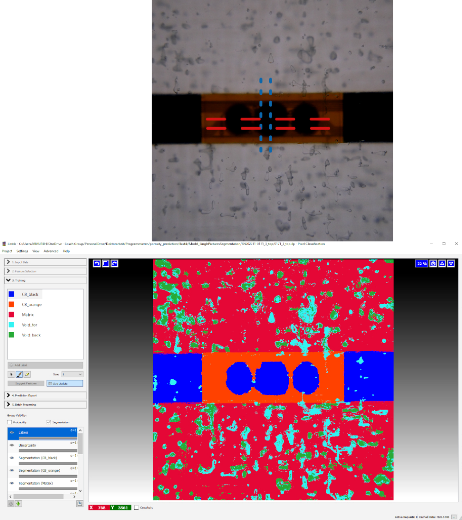

During early production, nine sensor neighborhoods were selected based on visual clues to likely cover the expected void content range. CT-samples of respective 35mm × 35mm were cut from the plates and CT-scanned with a diondo d5 system. This resulted in a resolution of 18μm/voxel, a value similar to references ^41,42 and approximately matching the fiber diameter. The measurement uncertainty was 2voxel, or 36μm. The minimum voxel size for voids was set to 50voxel, that is approximately 3.7voxel, respectively 66μm, side length under cubic shape assumption or 4.6voxel, respectively 82.3μm, diameter for spherical shape. These values aligned well with the measurement uncertainty. Although the CT-scans had lower resolution than the camera, they still provided better images than the camera due to the layered scanning of the material with minimal blur. However, according to these values, the CT-scans could also not detect micro-voids. The gray-scale threshold was set to 310 in a 16bit-system, whereby voids should have values below.

The first step in computing void content estimates was to segment the nine CT-samples’ pictures with the Pixel Classification workflow from the software ilastik⁴³. Two segmentation types were generated, which later served as hyperparameter for a regression model. Both consisted of ”Circuit board black”, ”Circuit board orange”, ”Matrix” as well as either the combination of ”Foreground void” and ”Background void” or simply ”Void”. An exemplary comparison between a camera picture and its segmentation, of the first type, can be seen in Figure 3. For this task, ilastik internally uses Random forests (RFs) that are trained on one or more images with few manual pixel labels to segment the rest of these images and others.

Each CT-sample picture was labeled individually until visually satisfactory segmentations were achieved. Since there was no direct way to quantify the quality of the individual segmentations, they were validated together with the regression models, which map the top and bottom view segmentations of each sensor neighborhood to a void content. For this, a 3-fold Cross-Validation (CV) was set up as shown in Figure 4. Six samples each, that is 12 labeled pictures, were used to train ilastik. The software segmented these input images and the six unlabeled pictures from the other three samples. A regression model was then trained with the 12 segmentations of the ilastik training images and validated using the other six. The target void contents were calculated from the CT-scans. Necessary processing and computations are described below.

Figure 4.

Flowchart illustrating the 3-fold CV procedure combining the ilastik segmentations with the regression models. Subsequent to the CV performance estimation, a model was trained with all nine CT-samples.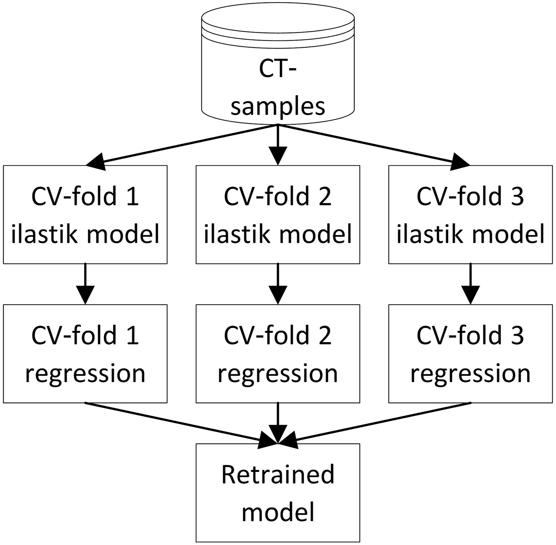

Although 35mm × 35mm pictures were segmented, subsequent computations used smaller centered 25mm × 25mm crops. This reduced the region of interest by 49%. As void height is an independent physical third dimension from area, it cannot be reliably estimated from 2d-pictures. Consequently, two types of proxy target values were generated and treated as hyperparameters. The first proxy was a naive summation of the projected void areas in the X-Y-plane as given by the CT-data. The other one was generated from artificial images where voids were approximated by circles with corresponding pixel ratios. These images were 2778px × 2778px, matching the pixel size of the cropped 25mm × 25mm pictures, maintaining the 9μm/px resolution. The void centers and radii were computed from the void coordinates and equivalent radii given by the CT-scans. Both kinds of area-based proxy targets are further justified by good correlation coefficients as follows: Due to the small number and non-random selection of samples, monotonic dependency between proxy values and volume-based void content was tested with Spearman correlations and Permutation tests that considered the alternative ”greater than the observed value”. The coefficients were approximately 0.98 and 0.95 for the naive summation and the circle-approach, respectively. Each test had a p-value of 0.0001. Additionally, the entire CT-data was tested for correlation of void areas and volumes as well as areas and heights. Thereby, Pearson’s correlation was used because of the large sample number and Permutation tests, with the alternative ”greater than the observed value”, were performed due to non-normality. The coefficients were approximately 0.9 and 0.74, respectively. The p-values were again 0.0001. These test results led to the conclusions that voids with a larger X-Y-area tend to have more volume and larger size in Z-direction, such that either proxy reasonably replaces volume void content.

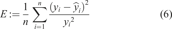
With respect to the 25mm × 25mm pictures, the corresponding volume void content, as given in the CT-data, was regarded as underlying ground-truth and used to split the samples for 3-fold CV. Subsequent to ilastik, regression models were trained and tested. Input features were derived from ratios of pixels segmented as void to the total pixel count. Further input options were based on the aforementioned two segmentation types, with and without the distinction into foreground and background voids, leading to different feature selections and interaction terms. An additional hyperparameter was the option to calculate the features after trying to fill voids that were only outlined by ellipses or horseshoes. The necessary parameters for the respective algorithm were tuned only once by the authors through visual comparison of the 18 segmentations and their original images. The regression targets were the area-based void content values obtained from either the naive summation or the circle-approach. Given the expectation of a linear relationship between segmentations and target values, a Linear regression (LR) was the first approach for a regression function. A concatenation of the function max(⋅, 0) with a linear one, implemented using a single ReLU-neuron within a NN framework, was also considered. It was expected that the neuron could better handle segmentation fragments or leftover dirt and scratches in the material that were segmented as voids. In this context, the maximum-function would provide a cut-off threshold if the parameter for a constant input feature were negative. LR models were optimized as usual by Mean square error, whereas ReLU-neurons were trained with the following error function, referred to here as Mean square relative error (MSRE), as loss function:

E : = \frac{1}{n} \sum_{i = 1}^{n} \frac{{(y_{i} - {\hat{y}}_{i})}^{2}}{{y_{i}}^{2}}

(6)

n is the number of considered samples, y_i are the target void contents and

{\hat{y}}_{i}

denote the corresponding estimates. This error function was chosen because small absolute deviations for small target values could result in a large relative errors. Since it is well-suited to combine errors for small and large targets, the MSRE was also used as performance measure for LRs and ReLU-neurons. Another performance measure was the Adjusted R², which is the variance in the targets explained by the inputs and penalized for increasing feature numbers. With the limited CT-data in mind, ilastik and the two respective best regression models were retrained on all nine CT-samples. As will be presented in the second Results and discussion section, it was decided to use the ReLU-neuron to compute void content from segmentations. Using the retrained neuron, estimates were assigned to the remaining 342 − 9 = 333 sensors.

Subsequent to these computations, a threshold was required to categorize the sensors, respectively their time series signals, as good or bad. Therefore, the naive summed area void contents were related to volume void contents by fitting a straight line, without intercept, to the CT-data, as can be seen in Figure 5. The data point with the highest volume void content is located at approximately 0.65% for the 25mm × 25mm crop and 0.63% for the original 35mm × 35mm sample. This particular sample is also the one shown in Figure 3. Since the material appears highly porous and the CT-data does not even contain 1% void content, the value 0.5%^35,36 was chosen among the thresholds presented in the Introduction. The corresponding area threshold was rounded to 10.7%. Applying it to the 323 sensors that recorded their RTM processes resulted in an imbalanced data set consisting of 283 good sensor neighborhoods, respectively signals, and 40 bad ones.

Figure 5.

Area void content and volume void content of the nine CT-samples within the 25mm × 25mm cropped region. The ReLU-neuron predictions are displayed as orange crosses. Its two largest relative errors are indicated by the dotted lines. The solid line represents the linear fit from volume void content to area void content that was used to the define the threshold, shown as dashed line. Based on a 0.5% volume void content, the corresponding area value was rounded to 10.7% and the dashed line points to the respective volume void content that is slightly lower than 0.5%.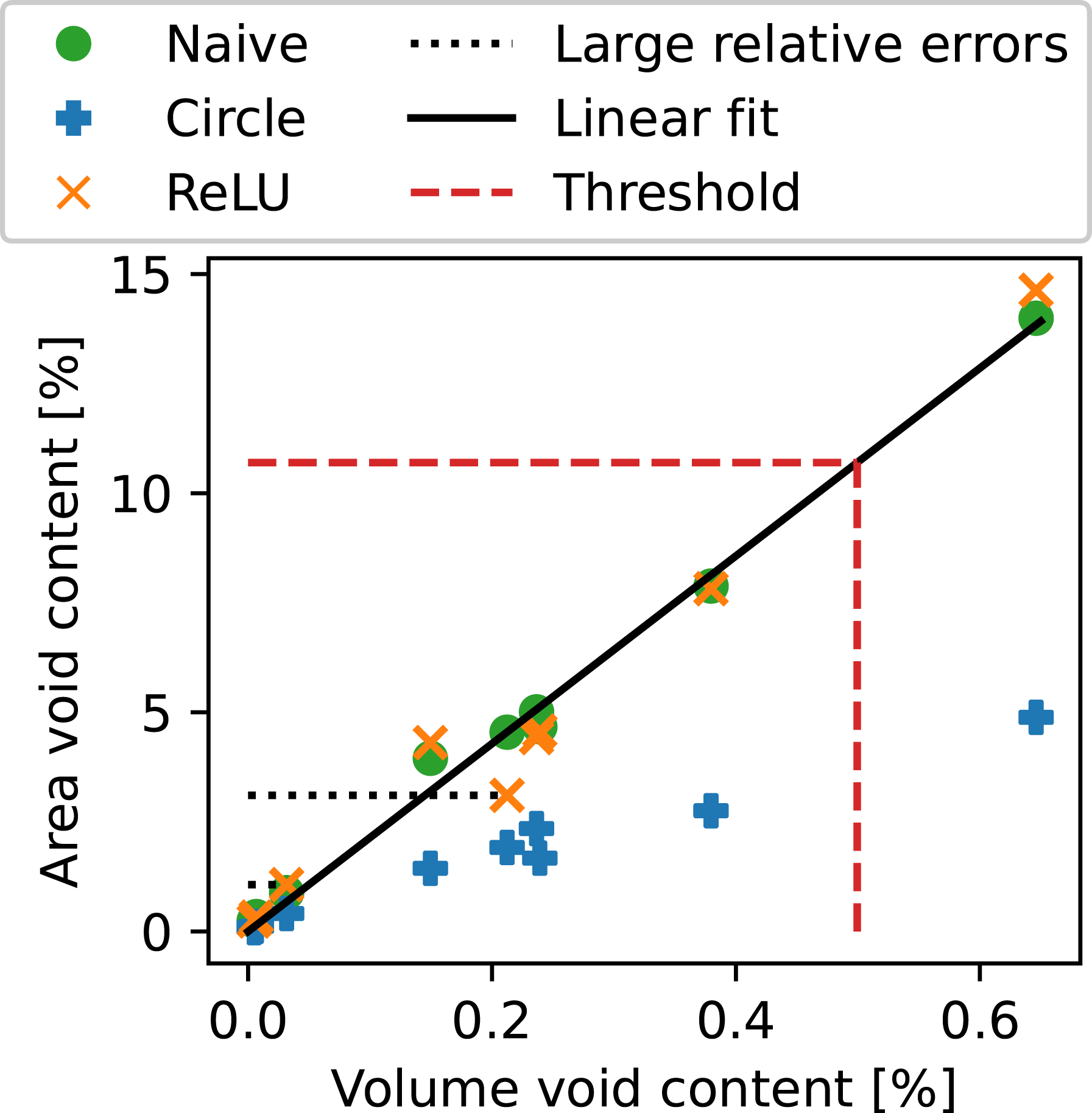

Void content classification from time series

Prior to processing and classification of the sensor signals, which are four-channel time series, the data was randomly split into a set for model-building and a hold-out set, while preserving class ratio. The latter was only used for final model testing. With an 80 : 20-split, the model-building set consisted of 258 sensors and the hold-out set of 65.

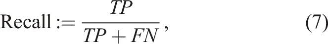
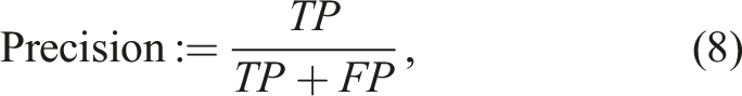
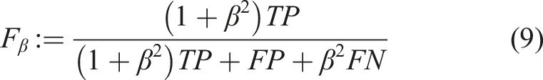
The classification task is intended as a quality control measure for produced components. The objective is therefore to detect bad samples and prevent them from further processing. This sample class was thus considered to be the one of interest, referred to as positive class. Contrary, good samples are called negative. Consequently, the number of false negatives needs to be low. The appropriate measure is Recall, defined as

Recall : = \frac{T P}{T P + F N},

(7)

where TP denotes true positives and FN false negatives. However, the classifier should be constrained to avoid generating a high number of false positives (FP). Therefore, the Precision, defined as

Precision : = \frac{T P}{T P + F P},

(8)

is not negligible. Recall and Precision are inversely related. Given this imbalanced problem, one of them had to be favored over the other. A measure that combines equations (7) and (8) while also providing a weighting between them is the so called F_β-score, defined as follows:

F_{β} : = \frac{(1 + β^{2}) T P}{(1 + β^{2}) T P + F P + β^{2} F N}

(9)

Recall is favored over Precision for β > 1 and Precision over Recall for β < 1. The well known F₁-score corresponds to the harmonic mean. Given the brief motivation above, Recall was deemed more important than Precision. β was set to 1.14, with respect to the approximate 14%-ratio of positive to negative samples in the model-building set. The F_1.14-score was considered the main performance measure for model training. However, performance will be reported in terms of F_1.14, F₁, Recall and Precision. Moreover, some of the following data preprocessing steps and classifier design choices were made to increase Recall.

Similarly to ²⁰, each sensor’s four-channel time series data was converted to a tabular format before being passed to a classifier. Since the sensors had different orientations and were exposed to an approximately elliptical resin flow from the center inlet, due to the 2/2 twill textile, the sensor data was first preprocessed to uniform orientation. With respect to the coordinate system depicted in Figure 2, corresponding acceleration axes were multiplied by the factor −1 such that the resin flow excited the X-axis in the negative direction and Y in the positive. Z was rotated such that the positive direction aligned with earth’s gravity. Next, each sensor’s acceleration and temperature time series were processed by identifying and removing outliers found by the Local outlier factor (LOF)⁴⁴. LOF interpreted each sensor’s complete four-channel signal as 4d point cloud and identified outliers based on density information. Although such high-leverage points could correspond to events, this processing step smoothed signals by removing points that could influence and destabilize statistical features computed from the time series. Removed values were filled again by the mean of the respective time series values before and after. Subsequently, features were generated for the tabular format, listed in Table 1. With respect to equations (1) to (3), only information related to the volume averaged flow velocity

⟨v⟩

was available, obtainable through numerical integration and differentiation of the acceleration signals. However, the sensors were mostly fixed in their positions due to being woven into the textile. Therefore, mainly statistical summaries of acceleration and temperature data in the time domain, as well as frequency domain features for acceleration, were computed. The temperature and pure acceleration features were directly calculated after LOF-processing. The jerk features used a further linear interpolation to idealized 1600Hz and the velocity ones underwent additional smoothing by a moving average filter with a window size of 160, corresponding to 1/10s. Moreover, the interpolated accelerations were also used for the frequency features. Some of these were based on the Power spectrum and Power spectral density (PSD), drawing inspiration from ⁴⁵. Others were computed using a Discrete wavelet transform, applying a 10-level decomposition to the last 36s corresponding to the flushing stages. Thereby four downward and four upward peaks were expected, recognizable in Figure 1, and their absolute values were considered. The computations yielded a total of 214 features. A later feature reduction was performed using a correlation threshold. Prior to this, Synthetic minority oversampling technique (SMOTE)⁴⁶ was performed on the model-building data. This aimed to mitigate the existing strong class imbalance and increase the number of positive samples without directly creating duplicates. In this context, a positive effect on Recall was expected. It was a design choice to oversample the positive class by three times its size, that is 32 + 3 ⋅ 32 = 128. This corresponded to approximately 56.6% of the negative class, respectively 36.2% of the augmented model-building data. Subsequent to SMOTE, the feature correlation matrix was computed. All columns with at least one correlation stronger than 80% in the upper right triangle, excluding the diagonal, were removed. This step reduced the feature number to 63, shown in Table 2, and concluded the data preprocessing.

Table 1.

Computed features where X, Y and Z denote the acceleration axes and T the temperature data. In the time domain, the first block refers to acceleration data only. For this block, the features of rolling data were generated for each window size of 50, 100, 200, 400, 800 and 1600. The second block combines acceleration and time through integration to velocity. Conversely, the third block combines both as a derivative to obtain jerk. For the frequency domain, the features in the first block were computed from the Power spectral and the Power spectral density (PSD). The respective second block was extracted from 10-level decompositions of the signals’ last 36s by applying Discrete wavelet transforms, where the eight peaks of the flushing stage were considered.

Acceleration time domain	Frequency domain	Temperature and others
Mean [X, Y, Z]	PSD strongest peak freq. [X, Y, Z]	Mean [T]
Standard deviation [X, Y, Z]	PSD 2^nd strongest peak freq. [X, Y, Z]	Standard deviation [T]
Standard dev. last 36s [X, Y, Z]	PSD 3^rd strongest peak freq. [X, Y, Z]	Maximum [T]
Maximum [X, Y, Z]	PSD strongest peak freq. last 36s [X, Y, Z]	Minimum [T]
Minimum [X, Y, Z]	PSD 2^nd strongest peak freq. last 36s [X, Y, Z]	Range [T]
Range [X, Y, Z]	PSD 3^rd strongest peak freq. last 36s [X, Y, Z]	Max. dev. from start [T]
Max. dev. from start [X, Y, Z]	Spectral entropy [X, Y, Z]	Median [T]
Median [X, Y, Z]	Spectral entropy last 36s [X, Y, Z]	Skewness [T]
Skewness [X, Y, Z]	Area under the power spectrum [X, Y, Z]	Kurtosis [T]
Kurtosis [X, Y, Z]	Median frequency [X, Y, Z]	Inter quartile range [T]
Inter quartile range [X, Y, Z]	Median frequency last 36s [X, Y, Z]	Mean absolute deviation [T]
Mean absolute deviation [X, Y, Z]	Special edge frequency [X, Y, Z]	Root mean square [T]
Root mean square [X, Y, Z]	Special edge frequency last 36s [X, Y, Z]
Energy [X, Y, Z]	Relative delta power [X, Y, Z]	Total duration [Time]
Energy last 36s [X, Y, Z]	Maximum power [X, Y, Z]
Mean of rolling means [X, Y, Z]	Mean power [X, Y, Z]
Mean of rolling standard devs. [X, Y, Z]	Standard deviation power [X, Y, Z]
Mean of rolling maxima [X, Y, Z]
Correlation [X to Y]	Level 10 approx. mean of peaks [X, Y, Z]
Correlation [X to Z]	Level 10 approx. standard dev. of peaks [X, Y, Z]
Correlation [Y to Z]	Level 10 details mean of peaks [X, Y, Z]
	Level 10 details standard dev. of peaks [X, Y, Z]
Final velocity [X, Y, Z]	Level 9 details mean of peaks [X, Y, Z]
Mean velocity [X, Y, Z]	Level 9 details standard dev. of peaks [X, Y, Z]
Standard dev. velocity [X, Y, Z]
Maximum velocity [X, Y, Z]
Minimum velocity [X, Y, Z]
Range velocity [X, Y, Z]

Mean jerk [X, Y, Z]
Standard dev. jerk [X, Y, Z]
Maximum jerk [X, Y, Z]
Minimum jerk [X, Y, Z]

Table 2.

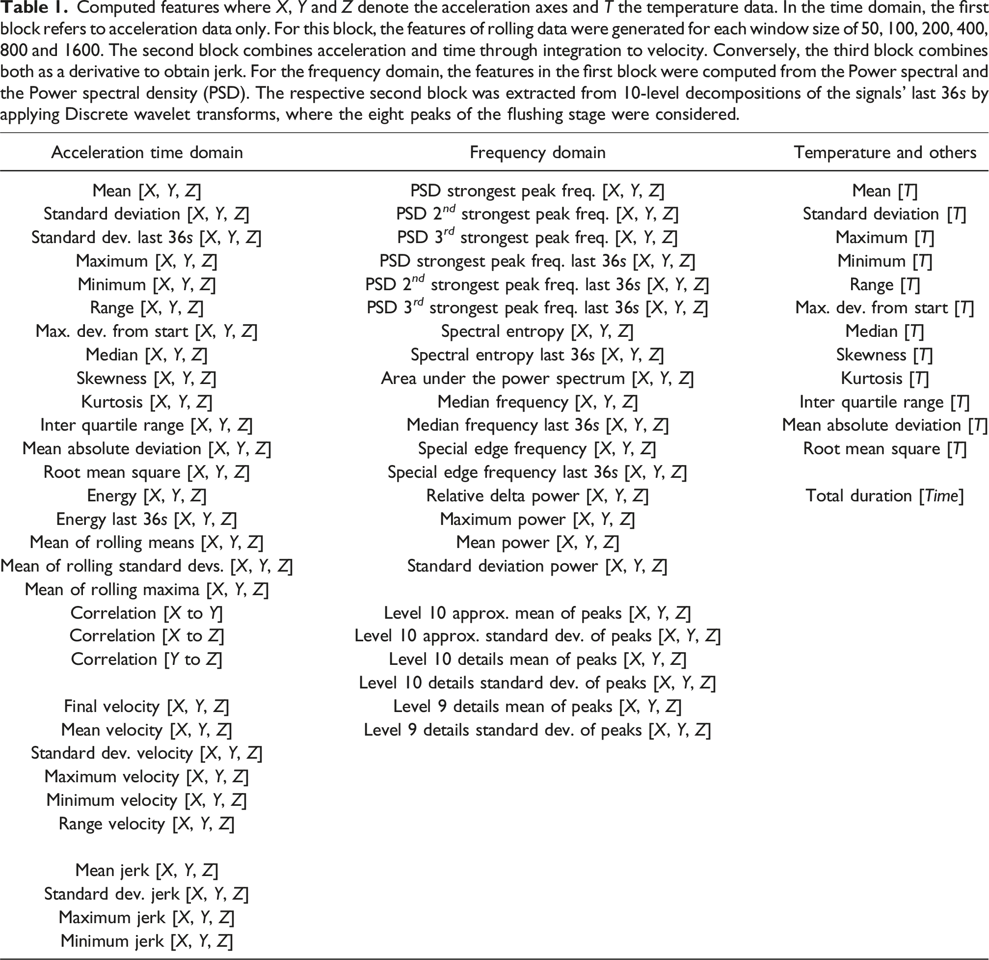
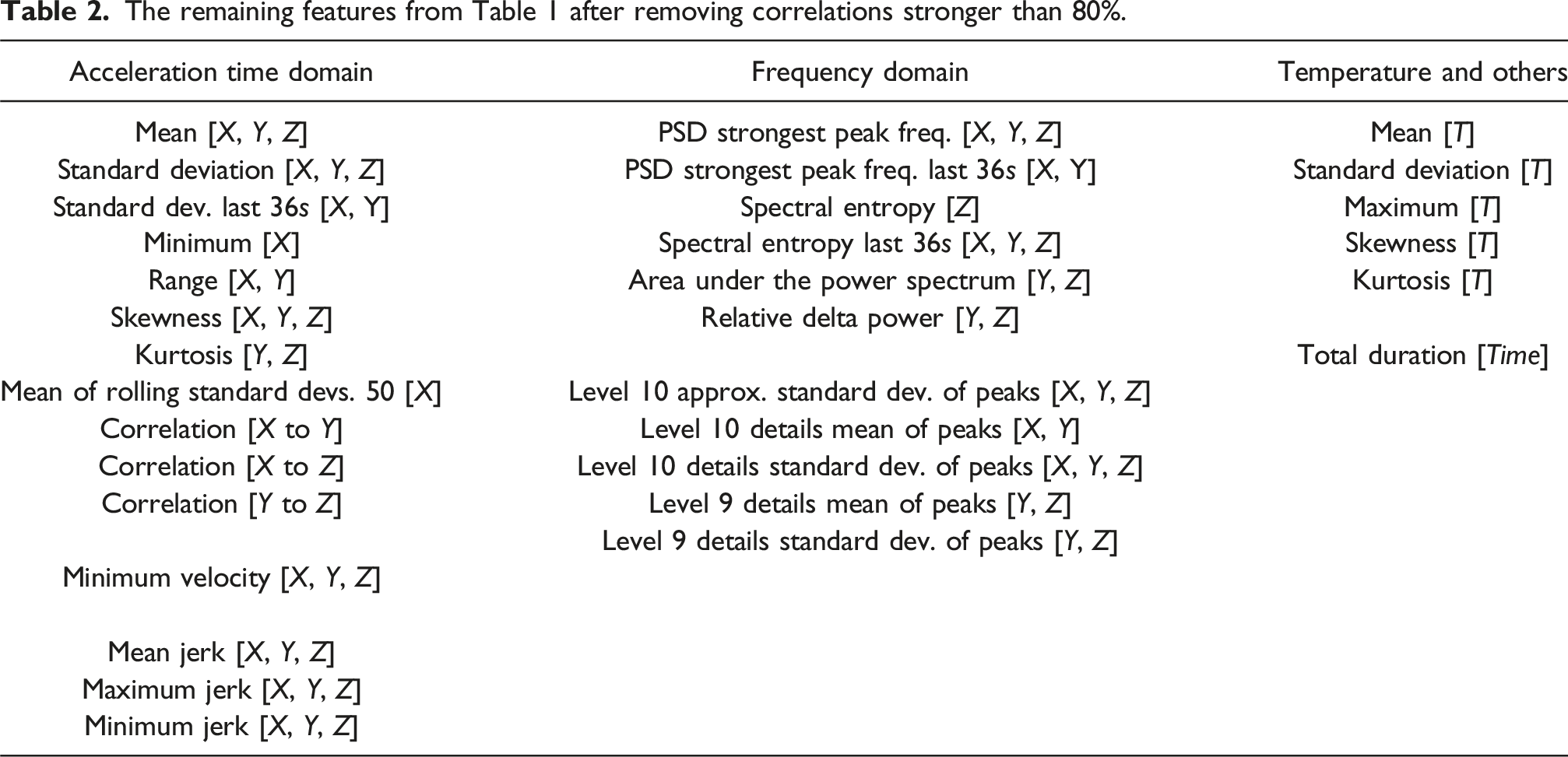
The remaining features from Table 1 after removing correlations stronger than 80%.

Acceleration time domain	Frequency domain	Temperature and others
Mean [X, Y, Z]	PSD strongest peak freq. [X, Y, Z]	Mean [T]
Standard deviation [X, Y, Z]	PSD strongest peak freq. last 36s [X, Y]	Standard deviation [T]
Standard dev. last 36s [X, Y]	Spectral entropy [Z]	Maximum [T]
Minimum [X]	Spectral entropy last 36s [X, Y, Z]	Skewness [T]
Range [X, Y]	Area under the power spectrum [Y, Z]	Kurtosis [T]
Skewness [X, Y, Z]	Relative delta power [Y, Z]
Kurtosis [Y, Z]		Total duration [Time]
Mean of rolling standard devs. 50 [X]	Level 10 approx. standard dev. of peaks [X, Y, Z]
Correlation [X to Y]	Level 10 details mean of peaks [X, Y]
Correlation [X to Z]	Level 10 details standard dev. of peaks [X, Y, Z]
Correlation [Y to Z]	Level 9 details mean of peaks [Y, Z]
	Level 9 details standard dev. of peaks [Y, Z]
Minimum velocity [X, Y, Z]

Mean jerk [X, Y, Z]
Maximum jerk [X, Y, Z]
Minimum jerk [X, Y, Z]

To classify the data into good and bad, respectively negative and positive, XGBoost models⁴⁷ were chosen due to their effectiveness in ²⁰. Given the binary classification task, the Binary cross-entropy was chosen as the loss function. A Bayesian optimization procedure was implemented to tune a selection of hyperparameters by maximizing F_1.14. The number of estimators could be optimized as an integer in the range from 10 to 70 and the maximum estimator depth as an integer between 2 and 5. Both were used to restrict the model complexity and the number of parameters in consideration of the small data set. To enable the model to adapt to the positive class, the learning rate was optimized within the interval [0.001, 1] and the positive class weight within [1, 10]. Furthermore, the optimization was stabilized by computing the mean F_1.14-score of a 4-fold CV. This number was chosen to maintain the distribution of natural positives between model-building and hold-out data, which was known due to the stratified split at the beginning. The CV also decreased the risk of overfit with respect to one specific validation set extracted from the model-building data. After hyperparameter optimization, the XGBoost performance was estimated in terms of F_1.14, F₁, Recall and Precision by a new 4-fold CV on the model-building data. Performance and generalizability for new, unseen data were then assessed by training a new XGBoost instance using the entire model-building data and applying it to the hold-out data. Based on the results obtained, model behavior was analyzed as described in the second Results and discussions section.

Results and discussions

The first section of this chapter presents and discusses the void analysis from SEM-micrographs. The second section focuses on the regression models used to generate porosity estimates. However, given the importance of the labeling process for classification, which is the subject of the third section, relevant aspects will be revisited in that context.

SEM-micrograph analysis

Four CT-samples were analyzed with SEM-micrographs. With respect to Figures 3 and 5, samples with approximately 0.149% and 0.005% volume void content were scanned along the blue-dotted lines. Samples with 0.239% and 0.007% were scanned along the red-dashed lines. SEM-imaging used a Zeiss Sigma VP at 5.00kV voltage. The working distance varied slightly around 7mm per material sample. All raster images were 2048px × 1536px. Appendix Figures (A1) to (A4) show overviews at 100× magnification, that is 0.56μm/px. Sensors are masked black and capacitors are displayed in white. The Loctite Eccobond encapsulation around them along with the circuit boards are also visible. The 2mm sensor width provides scale reference for the top images, while black 5mm scale bars are superimposed in the bottom images.

These figures demonstrate that the sensors and capacitors locally compact fiber tows but also provide inter-tow channels and resin rich pockets. The fiber tows in the blue-dotted markings were analyzed for V_f and the average matrix-area size between fibers via gray-scale analysis tools in Fiji software⁴⁸. From Figures (A1) to (A4), the V_f-values are 78.4%, 75.5%, 76.8%, and 74.8%, an increase from the reference of 55.8%. The average matrix cross-section area was measured as 201.3px, 237.9px, 267.1px, and 324.8px, corresponding to equivalent diameters of 6.3μm, 6.9μm, 7.3μm, and 8μm, respectively. Hence, average-sized micro-voids in these areas remain undetectable by camera and CT-scanning.

Multiple factors influence void formation, including preform microstructure, preform geometric anisotropy, resin flow direction, Ca*, and capillary pressure³. Voids can then migrate between inter- and intra-tow, split, merge and even diffuse into the resin^39,49,50. Therefore, a detailed assessment of how the sensors influence void formation is beyond this work’s scope. Nevertheless, sensors create competing effects on void formation. Local inter-tow channels reduce viscous flow resistance, promoting micro-void formation in nearby tows. Conversely, meso-voids may get trapped due to altered preform structure. Additionally, local fiber compaction increases the capillary pressure, which is known to decrease the micro-void content⁵¹. To investigate these effects, the red-dashed areas in Figures A1 and A2 were additionally scanned with 500× magnification, that is 0.11μm/px. As noted above, curing under increased pressure compressed voids after infiltration. However, the recorded data still shows a higher cross-sectional micro-void content with larger voids in less compacted areas. Exemplary images are displayed in images 1) to 7) of Figure 6. Image 8), extracted from Figure A4 at 100× magnification, demonstrates that voids can also occur at the resin-sensor interface. In image 1), all void-widths are smaller than 6.2μm, including the meso-void near the top. The gaps between fibers and matrix in 2) are fiber-matrix debonding with widths exceeding the image frame and large enough for CT-resolution. The large void in 3) has a width of 72.7μm, while the two ellipsoidal micro-voids below are smaller than 1.2μm. In 4), the larger void at the top left has an overall width of 13μm. Image 5) shows void clusters. The left is 50.3μm wide, the right one 20.6μm. The individual voids in the left cluster are wider than the camera resolution but not CT, whereas those on the right are neither. The void marked in 6) has a width of 10.6μm. In image 7), the left void is 25.6μm wide, while the smaller ellipsoidal void directly to the right measures only 2.5μm. Finally, the meso-void in 8) is 12.8μm wide, whereas the void at the resin-sensor interface has a width of 117.8μm. All these voids may not have been cut at their widest cross-section. However, comparison of the micro-voids in tows transversal to the plane against through the plane shows that even if one dimension exceeds 9μm, such as for images 3) and 7), the other one might be smaller than this value. Such voids would remain undetected by the camera. Moreover, the camera measurement uncertainty further reduces micro-void detectability. Analogously, voids with at least one dimension smaller than 18μm would also not be detected by CT-scans. For example, the wide voids in images 3) and 7) would not be detected based on the equivalent diameters calculated above and the void-widths from images 1), 4), 5) and 6). In contrast, both images in Figure A1 and the bottom image in Figure A3 show meso-voids for which an ellipsoidal shape is a reasonable assumption. In this order, these voids have widths, respectively one axis when viewed from above, of 133.5μm, 154μm, and 96.6μm. They were hence large enough for the camera and CT-scan resolutions.

Figure 6.

Detailed SEM-micrographs for various sections of the regions marked in Figures (A1) and (A2). Noteworthy voids are highlighted in red. Besides images 2), 7) and 8), the others are from regions close to the borders of the marked areas. The bottom part in 2) is the mold of the respective sensor, the gaps between fibers and matrix are debonding. Image 8), extracted from Figure A4, shows that voids can also occur at the sensor-resin interface. Selected size measurements are provided in the main text-body. Image 8) was recorded at 100× magnification, the others at 500×.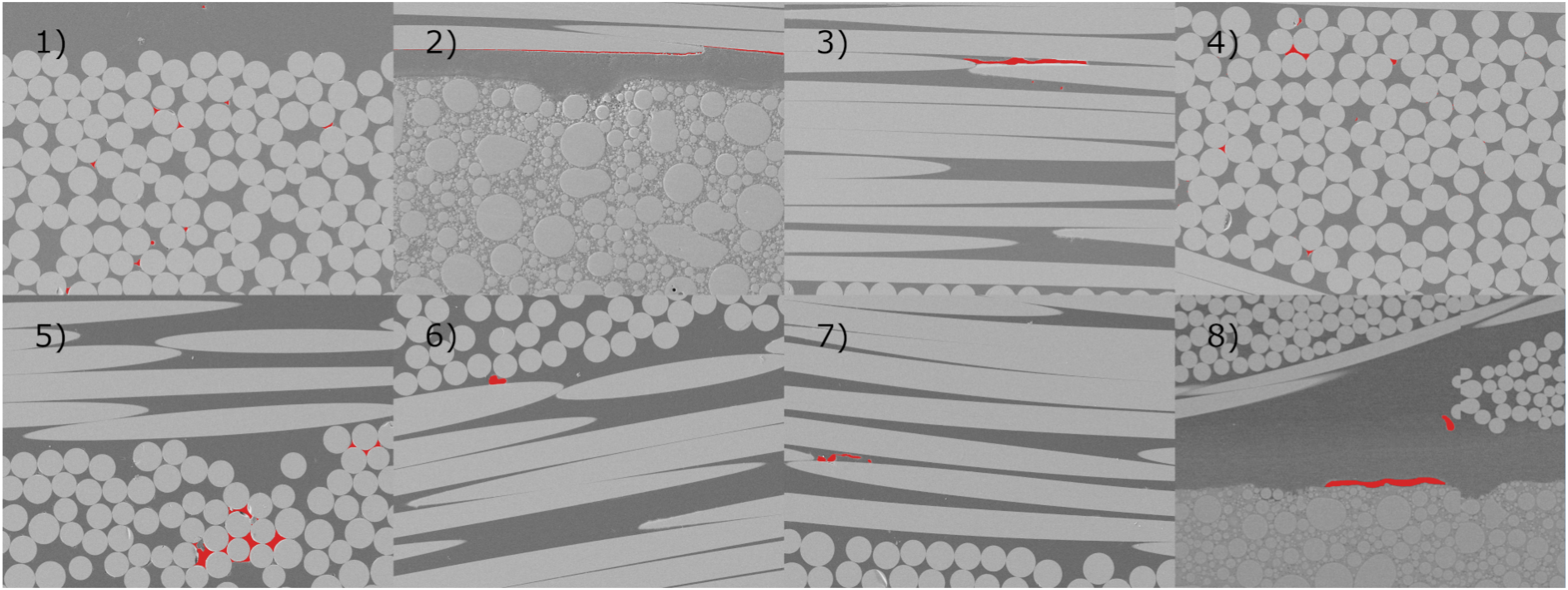

It was demonstrated that both CT-scans and photo box measurements overall underestimate the actual void content. Although one cannot distinguish between voids formed in sensor proximity and the ones transported there, micro-voids were found to be rare close to the sensors. Therefore, the two key assumptions that micro-voids transported intra-tow do not interact with the sensors, and that meso-voids rarely migrate into the tows³⁹, lead to the premise that the sensors mainly measure the viscous resin flow dynamics. The meso-void focused porosity measurements were therefore deemed reasonable for the present infiltrations where air entered the mold through the punctured inlet tube.

Regression models for labeling

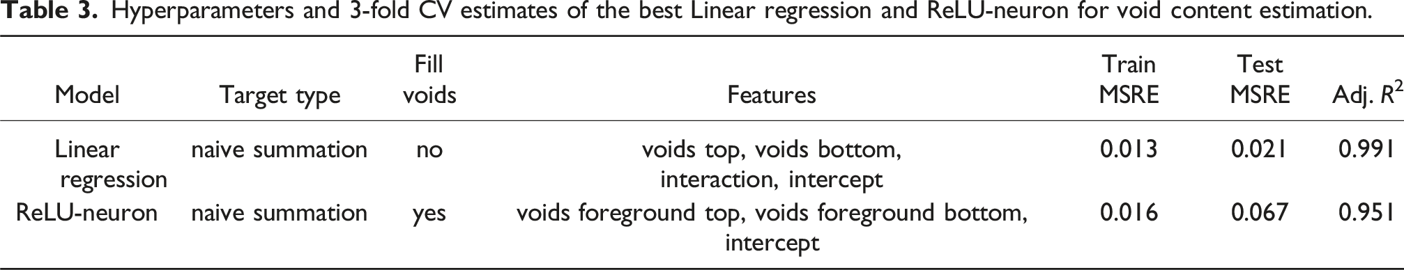
The neighborhood pictures were segmented using ilastik and subsequent regressions estimated void content. For this combined approach, the CV results and hyperparameters of the best performing LR and ReLU neuron are shown in Table 3. The retrained models’ performance values are displayed in Table 4. Additionally, Figure 5 shows the ReLU-outputs with respect to the corresponding volume void content.

Table 3.

Hyperparameters and 3-fold CV estimates of the best Linear regression and ReLU-neuron for void content estimation.

Model	Target type	Fill voids	Features	Train MSRE	Test MSRE	Adj. R²
Linear regression	naive summation	no	voids top, voids bottom, interaction, intercept	0.013	0.021	0.991
ReLU-neuron	naive summation	yes	voids foreground top, voids foreground bottom, intercept	0.016	0.067	0.951

Table 4.

Performance estimates of the Linear regression and ReLU-neuron that were retrained using all nine CT-samples.

Model	Train MSRE	Adj. R²
Linear regression	0.335	0.987
ReLU-neuron	0.019	0.968

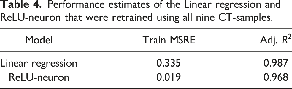
It can be observed from both tables that the performance of the final LR model decreased in comparison to the CV-estimates. Contrary, the ReLU-neuron performance increased in terms of Adjusted R² and decreased slightly in the training MSRE, but remained in the same order of magnitude. Besides the values reported in the tables, further factors led to the decision of using the ReLU-neuron. On the one hand, the LR had large relative residuals, the two most extreme ones being 0.74 and 1.54. It also produced negative outputs for inputs close to 0. On the other hand, the ReLU-neuron had smaller relative residuals. The two most extreme ones were 0.21 and −0.32, as indicated by the dotted horizontal lines in Figure 5. Obviously, the ReLU-neuron automatically restricted outputs to be greater than or equal to 0. Furthermore, the parameter value for the constant input was less than 0. It thus had the intended cut-off effect. However, this sometimes resulted in 0% void content for segmentations with only few, valid void pixels. Overall, these properties of the ReLU-neuron were considered advantageous compared to LR.

Figure 5 also illustrates that the ReLU-neuron itself made generalization errors. Although these occur naturally to some degree, it had to compensate for generalization errors made by the ilastik internal RF, as can be seen by comparing both images in Figure 3. Following this scheme, these errors were propagated to the classifiers, which will be discussed in the next section.

Void content classification

Regarding the XGBoost classifiers, the hyperparameter optimization resulted in 70 estimators with a maximum depth of 5. The learning rate was set to approximately 0.23 and the weight of the positive class was set to 1. Performance estimation through 4-fold CV is displayed in Table 5. The table also shows the hold-out performance of the XGBoost instance that was trained with the entire model-building data. The corresponding confusion matrix is presented in Figure 7. A noticeable performance decrease is evident for the hold-out data. In the following, this is used as a starting point for the model analysis. Thereby, it is important to note that the algorithms, especially the classifier, assume that good and bad, respectively negative and positive, sensor signals are sampled from two distinct underlying distributions. Consequently, they try to construct a possible classification boundary based on the available data. This indicates two main limitations that explain the model’ behavior and performances. The first limitation is the data set structure. In the following, multiple issues arising from it are conceptually introduced. To address and discuss them, a second iteration of XGBoost classifiers was trained. The other limitation are influences from the labeling process, which will be discussed afterwards. This section closes with an overall discussion and conclusion regarding the presented approach.

Table 5.

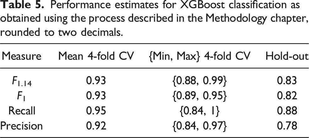
Performance estimates for XGBoost classification as obtained using the process described in the Methodology chapter, rounded to two decimals.

Measure	Mean 4-fold CV	{Min, Max} 4-fold CV	Hold-out
F _1.14	0.93	{0.88, 0.99}	0.83
F ₁	0.93	{0.89, 0.95}	0.82
Recall	0.95	{0.84, 1}	0.88
Precision	0.92	{0.84, 0.97}	0.78

Figure 7.

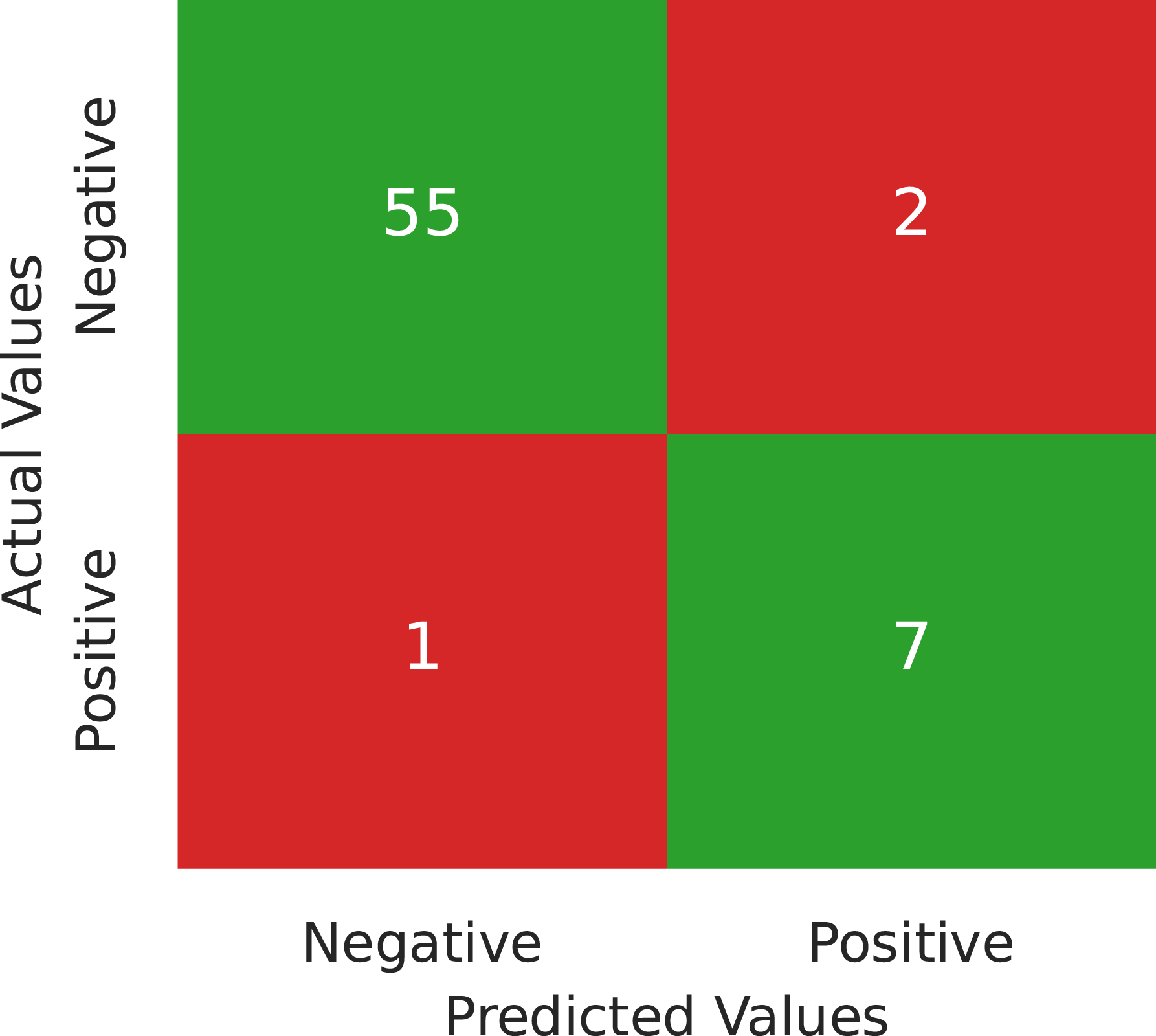
Confusion matrix for testing the XGBoost, trained with the entire model-building data as described in the Methodology chapter, using the hold-out data.

As mentioned in the Introduction, large data sets are usually required to obtain reliable AI-models. In contrast, the present data set both small and imbalanced. This gives rise to a mixture of different effects that impact model performance and performance estimation. First, the two assumed underlying probability distributions might not be sufficiently represented by the few available samples. In particular, the minority class, which is the positive one in this case, is typically most affected by this. Consequently, a classifier may favor the majority class over the minority class because it has more corresponding data available during training. To mitigate this, measures such as the application of SMOTE and the optimization of hyperparameters, in particular the positive class weight, with respect to the F_1.14-score were implemented. Another issue arising from such a data set is instability, meaning that model outputs for test data have a high variance with respect to changes in the training data. A relatively large number of features compared to the data set size can further contribute to this instability. Analogous to the Multiple testing problem in Statistics, a classifier may incorrectly attribute importance to features without good separation properties. This was likely the case with 63 features compared to only 258 natural model-building samples. Furthermore, the hyperparameters were optimized by CV on the model-building set. Although this approach was used to avoid them being specialized to one particular extracted subset, it overfitted them to the model-building data as a whole. This is because the different training and test sets in CV are not independent from each other. Additionally, this dependency is the reason why CV tends to overestimate model performance compared to an estimate based on an independent set, that is the hold-out set. Although CV is often used to obtain performance estimates for small data sets, the reliability of these estimates is compromised⁵². This effect was likely amplified by the hyperparameter optimization on the whole model-building data.

To address the aforementioned data set issues, a second iteration of XGBoost classifiers was trained. Since the amount and balance of the available natural data could not be changed, the methodology was updated. First, a new 80 : 20-split into model-building and hold-out data was generated. A nested CV was implemented to reduce the bias in the performance estimates with respect to the model-building data, replacing hyperparameter optimization and performance estimation through successive CVs. An inner 3-fold CV performed hyperparameter tuning through Bayesian optimization along with automated feature selection using the Maximum relevance minimum redundancy (MRMR) algorithm⁵³. As the name implies, MRMR identifies relevant features, here via F-statistics, and excludes redundant ones, here based on correlations. The earlier feature reduction based on the feature correlation matrix was thus omitted. The maximum number of features selected by MRMR was optimized as an integer between 3 and 7. The main XGBoost hyperparameter search space remained unchanged. The outer 4-fold CV included additional early stopping after 10 steps of no improvement for F_1.14 on the respective CV training sets. Results from the outer CV were used as performance estimates. To fit XGBoost to the whole model-building data and to evaluate on the hold-out data, the inner CV was performed once more on the model-building data. The maximum number of estimators resulted in 70, but early stopping restricted the final XGBoost to 31. The learning rate was optimized to approximately 0.36, the maximum estimator depth to four and the positive class weight to approximately 2.3. The performance values are summarized in Table 6. For this iteration, misclassifications on the hold-out data are reported, without additional confusion matrix, as follows: There was one false negative and three false positives.

Table 6.

Performance estimates for the second iteration of XGBoost classification after reducing the features, rounded to two decimals.

Measure	Mean 4-fold CV	{Min, Max} 4-fold CV	Hold-out
F _1.14	0.89	{0.87, 0.91}	0.79
F ₁	0.89	{0.87, 0.92}	0.78
Recall	0.89	{0.84, 0.94}	0.88
Precision	0.9	{0.83, 1}	0.7

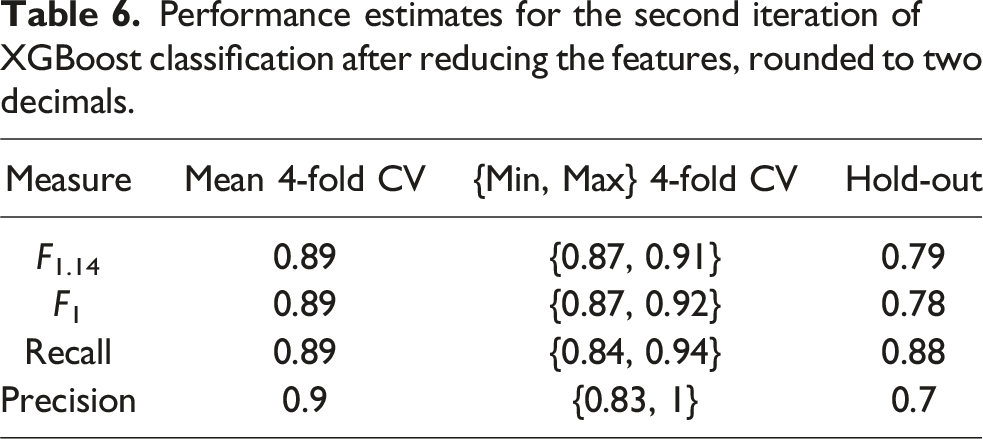
For this second iteration, the model fit was more reasonable than in the first one since hyperparameters did not reach the search space boundaries. Although the performance decreased again for the hold-out data, the nested CV estimates show decreased bias. This is visible in a slight decrease in mean performance as well as tighter estimate ranges and lower respective values for F_1.14, F₁ and Recall.

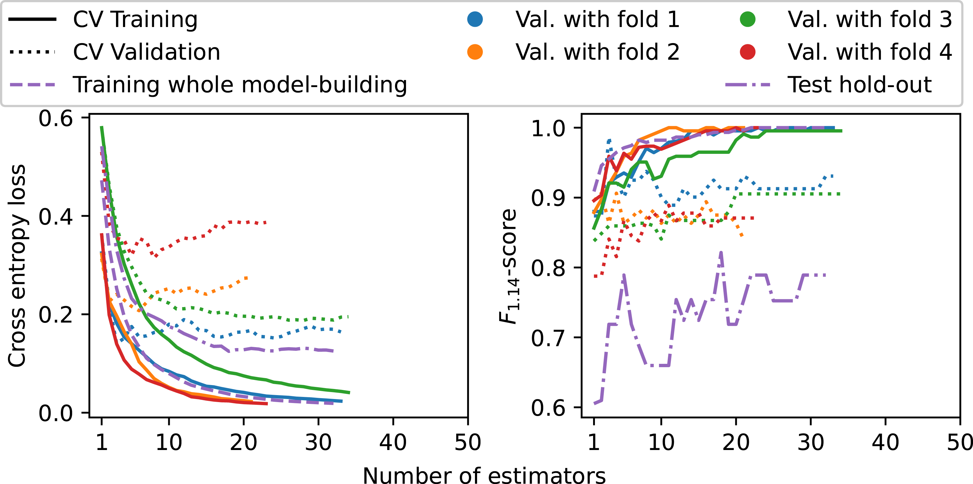
The new optimization approach also improved the class structure. The maximum number of features was set to 7, with final feature selection and corresponding F-statistics shown in Figure 8. All features are Z-axis features, and all except Standard deviation [Z] are in the frequency domain. A relevance drop occurs after the fifth most relevant feature, indicating that most information is carried by the top five and in the frequency domain. Nonetheless, all seven automatically selected features were used to train the second XGBoost classifier. Furthermore, Figure 9 shows the PCA-projections of both XGboost models trained on the whole model-building data. The plots were generated by projecting the data onto the respective model-building set’s two most important principal components after scaling the features to zero mean and unit variance. While the left-hand side plot for the 63 features does not show any structure, the right-hand side for the reduced seven features shows a cluster structure combined with improved class separation. This indicates that the high-dimensional feature space lost the class structure, whereas the 7d-case preserved it. Furthermore, the training graphs of the second XGBoost model are shown in Figure 10. The left-hand plot shows that the validation losses for folds 2 and 4 increased after a few estimators, while losses for folds 1 and 3 along with the hold-out test loss remained stable throughout respective model training. The right-hand plot demonstrates that early stopping prevented overfitting, as the F_1.14 validation and test curves do not show a clear overall decrease near training end. Despite the above described improvements, these curves further show some remaining model instability. With respect to the nested CV, the models with folds 1 and 2 for validation exhibit unstable training behavior, visible in the zigzag F_1.14 validation curves. Moreover, a strong discrepancy exists in the performance between validation folds 2 and 4 compared to folds 1 and 3. The final model trained on the whole model-building data shows on the one hand an overall increase in the F_1.14 test curve. On the other hand, this curve started on a lower value and failed to reach the bulk of the nested CV curves although the model had, after approximately 10 estimators, a test loss curve similar to the model with validation fold 1. The development of the F_1.14 test curve aligns with the overall performance drop for the hold-out data.

Figure 8.

Features selected by MRMR sorted by their relevance-score, that is the F-statistic.

Figure 9.

Samples projected onto the two most important principal components of the respective model-building sets. P denotes positive and N negative samples. T and F indicate true and false, respectively. Left: The first iteration XGBoost model, trained on the entire model-building data with 63 features, exhibiting no clear structure, Right: Corresponding XGBoost model trained with the reduced feature set from Figure 8, exhibiting a cluster structure and improved class separation.

Figure 10.

Training and validation, respectively test, curves for the second XGBoost iteration. The solid and dotted lines represent the outer four folds of the nested CV, whereas the retrained model on the entire model-building data and its test on the hold-out set are displayed in dashed and dash-dotted, respectively. Left: Binary cross-entropy loss, Right: F_1.14-score. The increasing validation losses and zigzag validation F_1.14 curves for fold 2 and 4 together with the worse zigzag hold-out test F_1.14 curve show remaining model instability.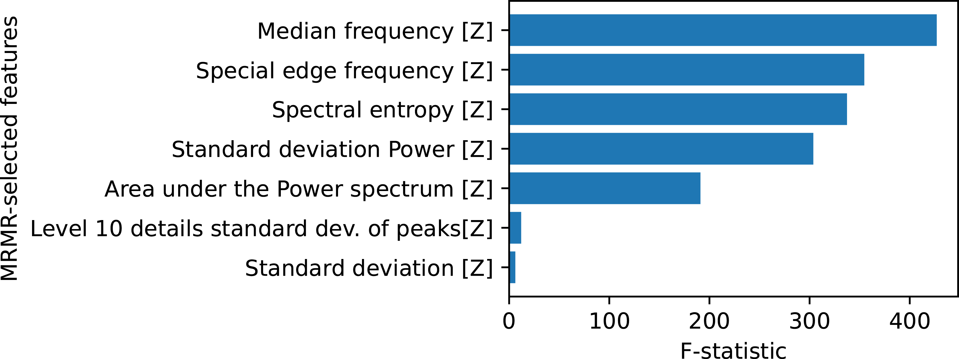

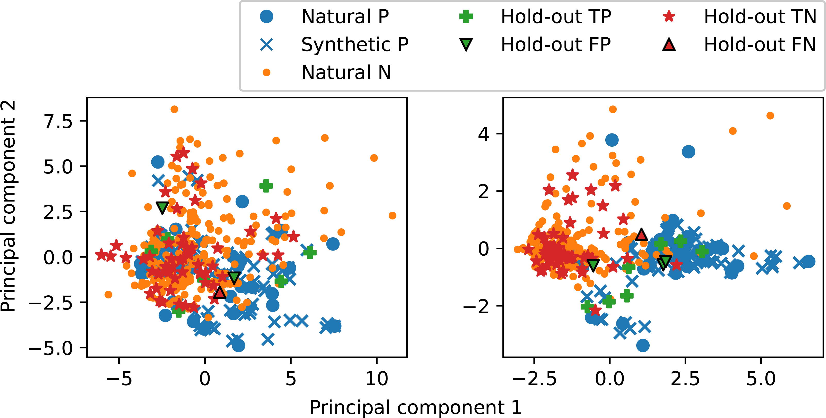
Each final XGBoost model’s hold-out misclassifications are also highlighted in Figure 9. These were traced back to their latent sample-IDs and area void contents. For the left-hand side plot, the central false positive had a void content of 9.28%, the one in the upper left had 0.61%, and the false negative had 19.65%. For the right-hand side, the leftmost false positive had 9.93% porosity, while the others had 0.41% and 4.42%, respectively. The false negative had 19.65% porosity. These values are consistent with the nine CT-samples’ porosity values. These findings reveal two distinct types of classification errors. The first type is due to the features’ separation capabilities for samples whose area void content is far from the threshold of 10.7%. Two hold-out samples for the first XGBoost, two false positives and the false negative for the second XGBoost belong to this. Such errors are likely avoidable with further feature engineering and even more hyperparameter optimization, as not all possible hyperparameters available to XGBoost were utilized in this study. The second type involves combined generalization errors from the labeling and classifier for samples near the threshold that can have different labels but similar signals. The first XGBoost model’s false positive with 9.28% and the second model’s false positive with 9.93% belong to this category. Although it is unlikely that the two assumed probability distributions are completely distinct, the labeling process influences their overlap. Hence, it also affects misclassifications. More sophisticated methods to estimate each sensor’s void content can help to reduce this overlap and consequently improve the classifier.

Overall, the classification performance and behavior was influenced by the data set size, class imbalance, and generalization errors propagated from the labeling process. These factors, however, would affect any classifier and not just the XGBoosts presented here. Class balance and data set size may improve through more production, whereby balance would be achieved by downsampling good samples rather than synthesizing bad ones and adjusting class weights. Performance improvement was therefore attempted by updating the methodology. Although major methodological changes to improve model performance were not explored, it has been demonstrated that the effects of the data set structure can be mitigated to some extent. Especially appropriate feature engineering and selection in the frequency domain appear to be a promising approach to extract void content information from the BMA456s′ acceleration data. Indeed, the reduction from 63 to seven features, six being frequency features, reduced classifier complexity and improved structure in the 2d-projected feature space. While the 63d-case exhibited no discernible structure, the 7d-case displayed a cluster structure with good visual separability between the two classes. Although the model instability was not fully solved and hold-out samples still misclassified, these results further support the potential of low-dimensional feature representations directly from the sensor data. Moreover, it is unlikely that generalization errors can be fully eliminated, regardless of the methods used for labeling. In this work’s main methodological reference ²⁰, a balanced data set of 10,000 pressure curves was processed, from which 2000 were held out for testing. These authors achieved 85.39% Recall and 82.92% Precision with their XGBoost model, respectively 83.69% and 81.35% with their LightGBM model. Therefore, the present performance estimates through nested CV and hold-out performance were considered acceptable. Moreover, even if the classification could be improved with further effort, the initial hypothesis that the BMA456 sensors capture void content information during RTM has been supported by the findings of this study.

Conclusions

GFRPC plates with embedded BMA456 acceleration sensors were fabricated using RTM. The hypothesis that the sensor data intrinsically captures void content information was investigated through binary classification of sensor data. After production, sensor neighborhoods were photographed with a self-built photo box. The resulting pictures were segmented using the software ilastik and a subsequent ReLU-neuron estimated the void content. Since porosity was generated from air introduced into the mold, the adequacy of this meso-void focused measurement was confirmed through SEM-micrographs, which show that micro-voids are rare in sensor proximity. The sensor signals were subsequently categorized as good and bad based on a threshold of 10.7% area void content, corresponding to 0.5% volume void content. This resulted in an imbalanced data set consisting of 323 sensor signals. Transformations from time series data into a tabular format were performed and XGBoost classifiers were applied. While the final classifier achieved good performance estimates through CV on the training data, exceeding mean values of 89% in the main metrics F_1.14, F₁, Recall and Precision, it suffered a performance decrease on an unseen, hold-out data set to F_1.14 ≈ 79%, F₁ ≈ 78%, Recall ≈ 88% and Precision = 70%. Model analysis revealed that this was primarily attributable to the data set structure, leading to inherent model instability, and propagated generalization errors from the labeling process. Consequently, the considered data set and approach limit further research with respect to void content. Researchers attempting a similar task with non-simulated data, respectively data from physical experiments, should design their experiments to obtain a balanced data set. This, however, is complicated since inherent randomness in void generation cannot be eliminated. Nonetheless, feature analysis showed that the sensors captured void content information and that it can be accessed in the frequency domain. In this sense, the present study provides evidence that acceleration sensor embedded into FRPCs may not only be used for component monitoring purposes, such as impact detection, but also for quality control during production. Furthermore, a transition from laboratory to series production should resolve the issue of a small, imbalanced data set by balancing through downsampling. However, in a series production context, specific resin systems are required to meet component mechanical properties, with resin flow optimized to minimize overall void content. Therefore, such resin systems should enable optimal modified capillary numbers that use a high resin velocity to exert higher forces upon sensor contact. Precise content measurement methods, available in series production contexts, would further help to reduce class overlap and thus generalization errors. Finally, this study focused only on local void content classification. Since embedded sensors create a wound effect in the components, they should not be placed along load paths where voids most significantly impact material performance. In this sense, a component wide quality control might be possible by combining local porosity estimates with resin velocity calculations in a respective sensor network.

Footnotes

Author note

Since completing the research with Robert Bosch GmbH, Markus Münch has changed employment to Bosch Sensortec GmbH, maintaining his affiliation with the University of Stuttgart. Vishesh Srivastava is currently a student at TU Dortmund University.

Acknowledgements

The authors thank all colleagues who were involved in technical discussions or support in the laboratory. They would like to pay special thanks to ARENA2036 e.V. for making the premises available for the production of the components. The authors are responsible for the contents of this publication.

ORCID iDs

Markus Münch

Vishesh Srivastava

Funding

The authors disclosed receipt of the following financial support for the research, authorship, and/or publication of this article: This study is anchored within the ARENA2036 research campus, funded by the German Federal Ministry of Education and Research (BMBF) within the framework of the project “Digital Fingerprint” (funding number: 02P18Q608) and coordinated by the Project Management Agency Karlsruhe (PTKA).

Declaration of conflicting interests

The authors declared no potential conflicts of interest with respect to the research, authorship, and/or publication of this article.

Data Availability Statement

The data and code that support the findings of this study are available from the corresponding author upon request.*

Appendix

References

Wazeer

Das

Abeykoon

, et al. Composites for electric vehicles and automotive sector: a review. Green Energy and Intelligent Transportation 2023; 2(1): 100043.

Peng

Zhang

, et al. Material performance, manufacturing methods, and engineering applications in aviation of carbon fiber reinforced polymers: a comprehensive review. Thin-Walled Struct 2025; 209: 112899.

Mehdikhani

Gorbatikh

Verpoest

, et al. Voids in fiber-reinforced polymer composites: a review on their formation, characteristics, and effects on mechanical performance. J Compos Mater 2019; 53(12): 1579–1669.

Simacek

Advani

. A numerical model to predict fiber tow saturation during liquid composite molding. Compos Sci Technol 2003; 63(12): 1725–1736.

Darcy

. Les fontaines publiques de la ville de Dijon: exposition et application des principes à suivre et des formules à employer dans les questions de distribution d’eau 1856. Victor dalmont, vol 1.

Labat

Grisel

Bréard

, et al. Original use of electrical conductivity for void detection due to injection conditions of composite materials. C R Acad Sci Ser IIB Mech 2001; 329(7): 529–534.

Facciotto

Simacek

Advani

, et al. Modeling formation and evolution of voids in unsaturated dual scale preforms in resin transfer molding processes. Compos Appl Sci Manuf 2023; 173: 107675.

Dev

Rahman

Islam

, et al. Properties prediction of composites based on machine learning models: a focus on statistical index approaches. Mater Today Commun 2024; 38: 107659.

Wang

Zhang

. Applications of artificial intelligence/machine learning to high-performance composites. Compos B Eng 2024; 285: 111740.

10.

Cui

La Spina

Fish

. Data-physics driven three-scale approach for ultra-fast resin transfer molding (uf-rtm). Comput Methods Appl Mech Eng 2024; 425: 116912.

11.

Fernández-León

Keramati

Miguel

, et al. A deep encoder-decoder for surrogate modelling of liquid moulding of composites. Eng Appl Artif Intell 2023; 120: 105945.

12.

Caglar

Broggi

Ali

, et al. Deep learning accelerated prediction of the permeability of fibrous microstructures. Compos Appl Sci Manuf 2022; 158: 106973.

13.

May

Syerko

Schmidt

, et al. Benchmarking virtual permeability predictions of real fibrous microstructure. In Proceedings of the American Society for Composites Thirty-Sixth Technical Conference on Composite Materials. DEStech Publications, Inc.

14.

González

Fernández-León

. A machine learning model to detect flow disturbances during manufacturing of composites by liquid moulding. Journal of Composites Science 2020; 4(2): 71.

15.

Hanna

Aguado

Comas-Cardona

, et al. A self-supervised learning framework based on physics-informed and convolutional neural networks to identify local anisotropic permeability tensor from textiles 2d images for filling pattern prediction. Compos Appl Sci Manuf 2024; 179: 108019.

16.

Fernández-León

Keramati

Garoz

, et al. A machine learning strategy for race-tracking detection during manufacturing of composites by liquid moulding. Integrating Materials and Manufacturing Innovation 2022; 11(2): 296–311.

17.

Zhu

Droste

Dimassi

, et al. A neural-network-assisted method for flow-front estimation in resin transfer molding using pressure sensors. J Compos Mater 2022; 56(19): 2979–2993.

18.

Chai

Eisenbart

Nikzad

, et al. Application of knn and ann metamodeling for rtm filling process prediction. Materials 2023; 16(18): 6115.

19.

Machado

Bodaghi

Nikzad

, et al. On the understanding of bubble dynamics through a calibrated textile-like porous medium using a machine learning based algorithm. Compos Appl Sci Manuf 2024; 177: 107955.

20.

Mendikute

Plazaola

Baskaran

, et al. Impregnation quality diagnosis in resin transfer moulding by machine learning. Compos B Eng 2021; 221: 108973.

21.

Di Fratta

Koutsoukis

Klunker

, et al. Fast method to monitor the flow front and control injection parameters in resin transfer molding using pressure sensors. J Compos Mater 2016; 50(21): 2941–2957.

22.

Gueroult

Lebel-Lavacry

Park

, et al. Analytical modeling and in situ measurement of void formation in liquid composite molding processes. Adv Compos Mater 2014; 23(1): 31–42.

23.

Zhao

Yang

, et al. Void content reduction of composites with sensor-aided injection strategy in liquid composite molding process. Mater Res Express 2021; 8(7): 075309.

24.

Neitzel

Puch

. Application of capacitive sensors and controlled injection pressure to minimize void formation in resin transfer molding. Polym Compos 2023; 44(3): 1658–1671.

25.

Torres

. Parameters’ monitoring and in-situ instrumentation for resin transfer moulding: a review. Compos Appl Sci Manuf 2019; 124: 105500.

26.

Rocha

Semprimoschnig

Nunes

. Sensors for process and structural health monitoring of aerospace composites: a review. Eng Struct 2021; 237: 112231.

27.

Jeong

Eum

, et al. In-situ resin flow monitoring in vartm process by using optical frequency domain reflectometry and long-gauge fbg sensors. Compos Struct 2022; 282: 115034.

28.

Liu

, et al. Leaky lamb wave-based resin impregnation monitoring with noninvasive and integrated piezoelectric sensor network. Measurement 2022; 189: 110480.

29.

Cui

Liang

, et al. Monitoring of three-dimensional resin flow front using hybrid piezoelectric-fiber sensor network in a liquid composite molding process. Compos Sci Technol 2022; 229: 109712.

30.

Holder

Middendorf

(eds). Digitaler Fingerabdruck. 1 ed., Springer Vieweg, 2025. ARENA2036.

31.

Bosch Sensortec GmbH . Bma456 - data sheet, march 2025. Document number: BST-BMA456-DS000-08. https://www.bosch-sensortec.com/media/boschsensortec/downloads/datasheets/bst-bma456-ds000.pdf

32.

Damm

Bahroun

Middendorf

. A low-cost flow front monitoring system. ICCM22 2019: 236–244.

33.

Münch

Bodke

Repphun

, et al. Rtm-flow front detection for gfrp components with embedded mems-acceleration sensors. Proceedings of the 21st European Conference on Composite Materials 2024; 8: 179–186.

34.

Damm

Spitzmüller

Raichle

ATS

, et al. Deep learning for impact detection in composite plates with sparsely integrated sensors. Smart Mater Struct 2020; 29(12): 125014.

35.

Purslow

. On the optical assessment of the void content in composite materials. Composites 1984; 15(3): 207–210.

36.

de Almeida

SFM

Neto

ZSN

. Effect of void content on the strength of composite laminates. Compos Struct 1994; 28(2): 139–148.

37.

Saenz-Castillo

Martín

Calvo

, et al. Effect of processing parameters and void content on mechanical properties and ndi of thermoplastic composites. Compos Appl Sci Manuf 2019; 121: 308–320.

38.

Bayat

Jamzad

Zobeiry

, et al. Temporal enhanced ultrasound: a new method for detection of porosity defects in composites. Compos Appl Sci Manuf 2023; 164: 107259.

39.

Aaboud

Saouab

Nawab

. Simulation of air bubble’s creation, compression, and transport phenomena in resin transfer moulding. J Compos Mater 2017; 51(29): 4115–4127.

40.

Yalcinkaya

Sozer

Altan

. Effect of external pressure and resin flushing on reduction of process-induced voids and enhancement of laminate quality in heated-VARTM. Compos Appl Sci Manuf 2019; 121: 353–364.

41.

Rosemeier

Lester

Antoniou

, et al. Determination of as-built properties of fiber reinforced polymers in a wind turbine blade using scanning electron and high-resolution X-ray microscopy. Composites Part C: Open Access 2022; 9: 100310.

42.

Kastner

Plank

Salaberger

, et al. Defect and porosity determination of fibre reinforced polymers by X-ray computed tomography 2nd international symposium on NDT in aerospace. https://www.ndt.net/?id=10410

43.

Berg

Kutra

Kroeger

, et al. Ilastik: interactive machine learning for (bio)image analysis. Nat Methods 2019; 16(12): 1226–1232.

44.

Breunig

Kriegel

, et al. Lof: identifying density-based local outliers. SIGMOD Rec 2000; 29(2): 93–104.

45.

Tonner

Bein

. Classic electroencephalographic parameters: median frequency, spectral edge frequency etc. Best Pract Res Clin Anaesthesiol 2006; 20(1): 147–159.

46.

Chawla

Bowyer

Hall

, et al. Smote: synthetic minority over-sampling technique. J Artif Intell Res 2002; 16(1): 321–357.

47.

Chen

Guestrin

. Xgboost: a scalable tree boosting system. In Proceedings of the 22nd ACM SIGKDD International Conference on Knowledge Discovery and Data Mining. Association for Computing Machinery, 2016, pp. 785–794.

48.

Schindelin

Arganda-Carreras

Frise

, et al. Fiji: an open-source platform for biological-image analysis. Nat Methods 2012; 9(7): 676–682.

49.

Frishfelds

Lundström

Jakovics

. Bubble motion through non-crimp fabrics during composites manufacturing. Compos Appl Sci Manuf 2008; 39(2): 243–251.

50.

Patiño Arcila

Power

Nieto Londoño

, et al. Boundary element method for the dynamic evolution of intra-tow voids in dual-scale fibrous reinforcements using a stokes–darcy formulation. Eng Anal Bound Elem 2018; 87: 133–152.

51.

Yeager

Hwang

Advani

. Prediction of capillary pressure for resin flow between fibers. Compos Sci Technol 2016; 126: 130–138.

52.

Varoquaux

. Cross-validation failure: small sample sizes lead to large error bars. Neuroimage 2018; 180: 68–77.

53.

Peng

Long

Ding

. Feature selection based on mutual information: criteria of max-dependency, max-relevance, and min-redundancy. IEEE Trans Pattern Anal Mach Intell 2005; 27(8): 1226–1238.

Void content classification for acceleration sensor embedded glass-fiber reinforced components made by resin transfer molding

Abstract

Keywords

Introduction

Materials and methods

Production process

Void content labels from images

Void content classification from time series

Results and discussions

SEM-micrograph analysis

Regression models for labeling

Void content classification

Conclusions

Footnotes

Author note

Acknowledgements

ORCID iDs

Funding

Declaration of conflicting interests

Data Availability Statement

Appendix

References