Sage Journals: Discover world-class research

Abstract

Composite-metal joints are usually implemented in the form of adhesive joints as there are well established best practices and theories of how to model them. In some cases, using the conventional method such as adhesive joint isn’t desirable, be it due to external environment or other factors. For the purpose of connecting two parts of a joint shaft (steel constant-velocity joint and fiber-reinforced polymer tube), a splined coupling was considered. The connection consists of a steel shaft with small splines on the contact surface with its FRP counterpart. The FRP tube has a smooth cylindrical surface and the steel splines cut into this material during a press-fitting process. This connection is referred to as the press-fitted spline joint (PFSJ). This paper presents a simplified yet surprisingly well-functioning analytical model of such a joint that calculates the damage of the joint and its torque capacity based on dimensions and materials. This model utilizes the theory of thick-walled cylinders, the classical lamination theory, and the Hashin damage criteria. Furthermore, a FEM model was proposed to verify the analytical model and to study the joint in more detail. Lastly, the models were compared to the data from the static torsion test. The most time-efficient and yet trustworthy way to model the behavior of the PFSJ is to use the slip-dependent friction model. The more precise way is to employ the exponential traction-separation law coupled with friction, which on the other hand converges slowly than the sole friction model.

Keywords

Press-fitting splined joint FRP filament winding

Introduction

The automotive industry faces significant pressure to reduce CO₂ emissions and improve the energy efficiency of vehicles. One of the ways to achieve it is through lightweighting by using composite materials also known as fiber reinforced polymers (FRP).^1,2 Car manufacturers have already utilized carbon fiber reinforced polymers (CFRP) into the vehicle structure³ with reasonable financial rentability.⁴

A suitable application for the automotive sector where components need to be produced on a large scale with a high level of automation is to employ the technology of filament winding. Several researchers have already developed hybrid metal/CFRP driveshafts.^5–7 This helped to achieve higher natural frequencies⁸ and better fatigue behavior.⁹ Proper use of CFRP can also reduce vehicle noise and vibrations^10,11 or even gearbox vibration.¹² The perspective of noise and vibration becomes important especially in electric vehicles where there is no internal combustion engine (ICE), which was the main source of noise and superimposed every other source.¹³

An ongoing project at Czech Technical University (CTU) in cooperation with industry partners Skoda Auto and CompoTech aims to develop the FRP joint shaft between the front and rear axle for a 4 × 4 vehicle with a promise of achieving lightweighting and also potential cost savings thanks to simplified design and manufacturing. One particular problem stands out during the development process. How to connect a steel constant velocity (CV) Rzeppa and tripod joints to the composite shaft? The obvious choice for such connection would be to use bonded joints that withstand average shear stress up to 45 MPa¹⁴ and the best practices are well known.¹⁵ However, in this particular application where the joint shaft is close to the exhaust pipe and the catalytic converter that might reach a temperature of hundreds of degrees Celsius and heat the shaft, the use of a bonded joint might not be the optimal solution. Adhesives are prone to lose mechanical properties due to external conditions such as high temperature,^16,17 hygrothermal exposure,¹⁸ combination of both¹⁹ or cyclic thermal conditions.²⁰ An inappropriate choice of adhesive can even lead to loss of strength by 75%. It is then reasonable to look for alternatives that are less affected by these conditions.

There are many ways to approach the problem. For example, using simple press-fit joints²¹ or bolting sleeves.²² Another option is to employ innovative designs such as the so-called integrated loop joints taking advantage of filament winding technology that allows to manufacture holes at the ends of the shaft without cutting the material,²³ or using fasteners with an adjustable interference²⁴ or various types of screw joints.^25,26

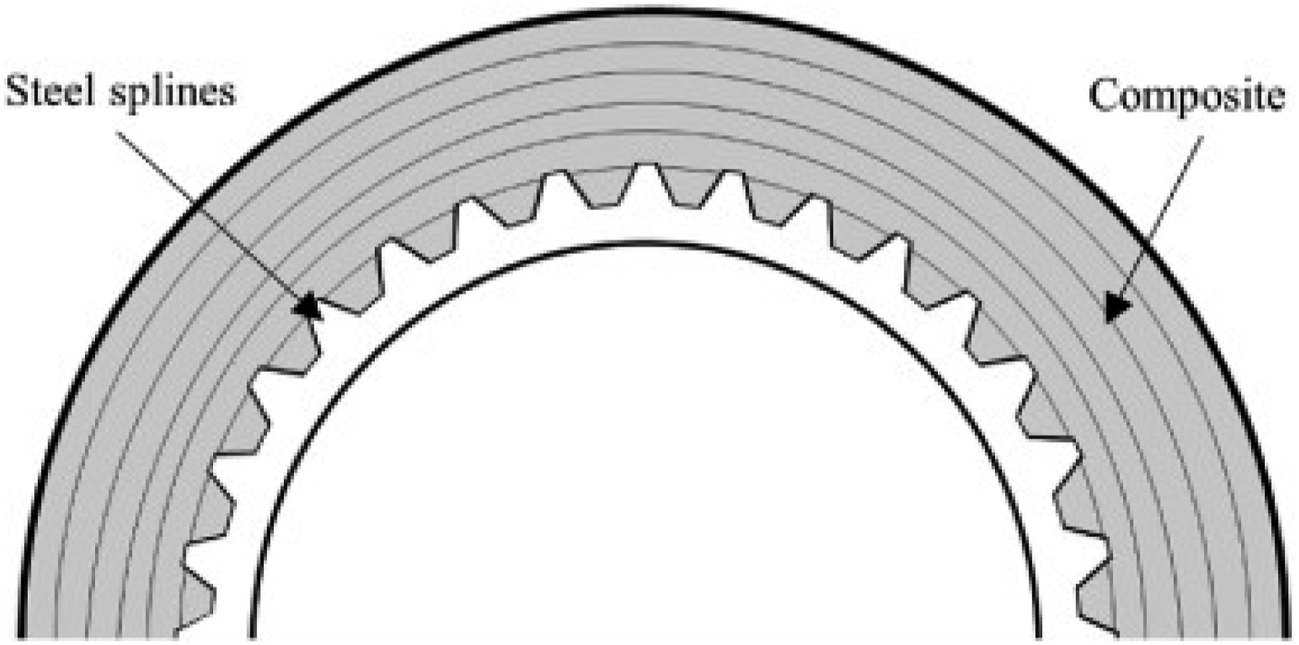
One particular solution stands out as the most suitable for the joint shaft, which is mentioned in a review by Jarrett et al.²⁷ The principle is shown in Figure 1. It is a method in which a metal end fitting contains small splines (not higher than 0.5 mm) on the contact surface with its composite counterpart. This end fitting is press-fitted into a smooth cylindrical surface of a composite tube, cutting the FRP during the press-fitting process and in the end forming a coupling capable of transmitting torque and also withstanding axial load as well. This is a very different mechanism in contrast to the most commonly used way of connecting metal and composite parts (adhesive joints) or to less common but simple methods such as mechanical fastenings. While adhesive joints or mechanical fastenings such as simple press-fitting or bolts may be referred to as conventional for the frequency of use or for their simplicity, this method on the other hand is, to the knowledge of the authors of this article, rarely used, and the mechanism with which the load is transferred is a combination of friction force (caused by press-fitting) and force carried by teeth and grooves. In addition, the assembly process itself damages the interfacial surface of the composite tube, which is very unusual. For these reasons, this joint is called unconventional. This method was chosen to connect steel CV joints to the FRP tube, as the absence of adhesive makes it less prone to external conditions such as cyclic thermal conditions and extreme temperatures. The increase in temperature (in a reasonable range) might even be beneficial to torque capacity as FRP have a negative coefficient of thermal expansion. The increased temperature expands the steel shaft and shrinks the FRP tube resulting in a higher contact pressure that allows the transfer of greater torque. For the purpose of this paper, this coupling will be referred to as a press-fitted splined joint (PFSJ).

Figure 1.

Schematic example of steel shaft with splines press-fitted into a composite tube.²⁷.

While knowing the principle of this coupling, there is an utter lack of information in any literature on how to approach the design of such a joint. Due to its complexity, it is difficult to presume its behavior with sufficient level of certainty. What load can the joint withstand with the chosen dimensions? How to model it? What is the stress state in the joint? These issues have to be addressed before this joint is used in a real application.

The objectives defined together with the project partners are:

• Create a simple analytical model that would serve as a quick tool for engineers (even for those with no deep knowledge of the damage mechanics of FRP) to design PFSJ based on load, dimensions, and other input parameters.

• Create an FEM model describing the same mechanical principle as the analytical model and use it to verify the functionality of the analytical model.

• Use the FEM model to investigate the influence of the reinforcing layer length on the joint’s load bearing capacity.

• Modify the FEM model to include detailed geometry of the teeth and study the influence of different geometrical parameters on the load bearing capacity.

• Conduct a static torsion test on a sample containing PFSJ to compare the obtained data with results from both analytical and FEM models.

• Based on the experiment, modify the simplified FEM model so the torque response includes damage initiation and damage progression, and therefore the behavior of the FEM model correspond with the experiment.

Concept of the joint

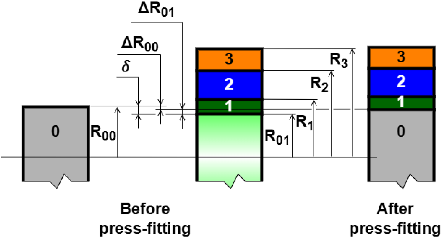
The design of the joint is inspired by a series of patents by Dewhirst,^28–30 Lewis and Dewhirst,³¹ Faulkner³² and Nakamura^33,34 that use a slightly different geometry of the splined shaft than the one shown in Figure 1. The proposed geometry will be described later in this chapter. The joint consists of a steel shaft and a composite tube with different layers, each serving a specific function. The component 0 in Figure 2 refers to the steel shaft with teeth on the surface. Components 1, 2 and 3 are layers of the composite tube.

Figure 2.

Concept of the joint.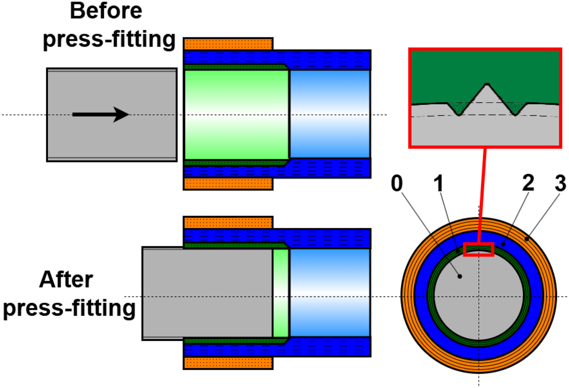

Layer 1 is a thin layer of glass fiber reinforced polymer (GFRP), designed to be approximately 1 mm thick (depending on the diameter of the shaft). Its purpose is to be cut by the teeth of the shaft and transmit the load to the subsequent layer. Using glass fibers in this layer is for several reasons. The first is that GFRP has better properties in terms of resistance to damage progression than CFRP. This is of great importance because during the press-fitting process, the teeth of the shaft initiate damage in the material, most likely brake fibers, and it is crucial not to allow this damage to progress further. Another reason for using glass fibers is to prevent a contact between steel and carbon fibers for these two materials can form a galvanic couple and degrade the joint. The orientation of the glass fibers in layer 1 is 90°, meaning the fibers are in the circumferential direction. Therefore, the load is transmitted interlaminarily.

Layer 2 is the one that is primarily meant to be connected to the input shaft. It transmits the load further into the drivetrain. In case of bonded joint, only the shaft and layer 2 would be used. Any fiber material and orientation can be used for this layer, depending on the purpose of the composite part and the applied load.

Layer 3 is a reinforcing layer. It consists of ultra high modulus (UHM) fibers oriented at 90° angle (circumferential direction). This layer increases the stiffness of the joint in the radial direction, meaning resistance to the increasing diameter of layers caused by press-fitting. When the shaft is press-fitted into the tube, it forces the tube to increase its diameter, and thus its circumference. But when UHM fibers in layer 3 are oriented circumferentially, they cause resistance against the expansion resulting in increased pressure between layers 0 and 1 which leads to higher load capacity.

Apart from presenting the overall concept of the joint and the process of press-fitting, Figure 2 along with Figure 3 show detail of the connection between layers 0 and 1 i.e. the shape of the splined shaft. While the Figure 1 shows only a schematic principle of the joint (teeth on shaft cut into composite tube), the proposed geometry is inspired by already implemented solutions that deal with practical issues. The splines have several traits. The first is that next to each tooth, there’s a surface with a diameter D which is the same as the inner diameter of the composite tube, helping to achieve the correct mutual position between the two parts during press-fitting and avoid eccentricity or misalignment. The diameter D_e defines the tooth height h_t indicating the extent to which the composite tube is cut by the teeth, which is crucial for achieving a sufficient grip to transfer the load. The internal diameter D_i provides space (h_g) for the composite material that is cut during the press-fitting to fill the groove. The angle of the tooth α_t is along with the parameter h_t crucial to influence the load bearing capacity. The angle φ adjusts the pitch of the teeth, and thus the total number of teeth on the circumference of the shaft. It should be chosen as a compromise between a high number of teeth (transferring higher load) and a sufficient centering surface D along with a sufficient distance of teeth tips in order to avoid higher stress. Radii r_t and r_g are influenced mainly by manufacturing constraints.

Figure 3.

Geometry of the splined shaft.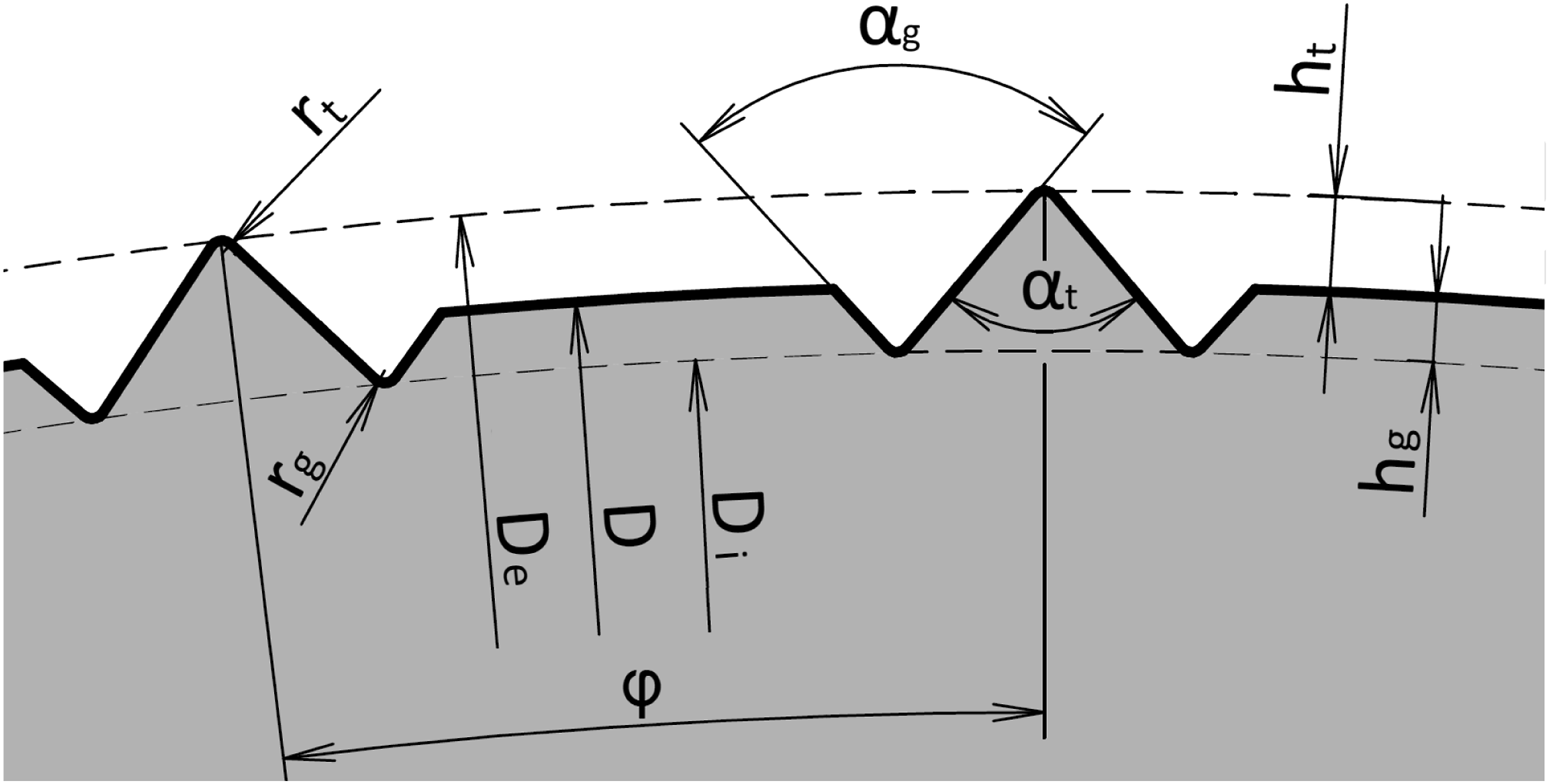

The press-fitting process itself consists of several phases. The first is aligning the two respective parts to ensure geometric precision. For this, either a short leading face with the same diameter as the inner tube diameter - D, or precise assembling fixtures are required. As the section of the shaft with teeth above diameter D reaches the tube, the teeth start to cut through the glass fiber composite layer, partly cutting its fibers and matrix, partly deforming the matrix and reorienting the fibers along the teeth. Excess material is pushed preferably to the sides into the grooves or in an axial direction. This causes a sudden increase in the pressing force. The shaft is then pushed further and the pressing force grows proportionally to the length of the insertion into the tube. This process requires using machine press as the forces can reach tens of thousands of Newtons.

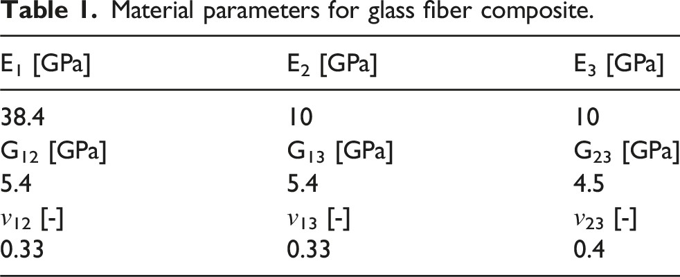
Tables 1–3 list the material parameters for individual layers. The parameters include Young’s moduli E, shear moduli G and Poisson’s constants ν in directions 1 (longitudinal), 2 (transversal), and 3 (in thickness). These parameters are used in all models that will be discussed in subsequent chapters.

Table 1.

Material parameters for glass fiber composite.

E₁ [GPa]	E₂ [GPa]	E₃ [GPa]
38.4	10	10
G₁₂ [GPa]	G₁₃ [GPa]	G₂₃ [GPa]
5.4	5.4	4.5
ν₁₂ [-]	ν₁₃ [-]	ν₂₃ [-]
0.33	0.33	0.4

Table 2.

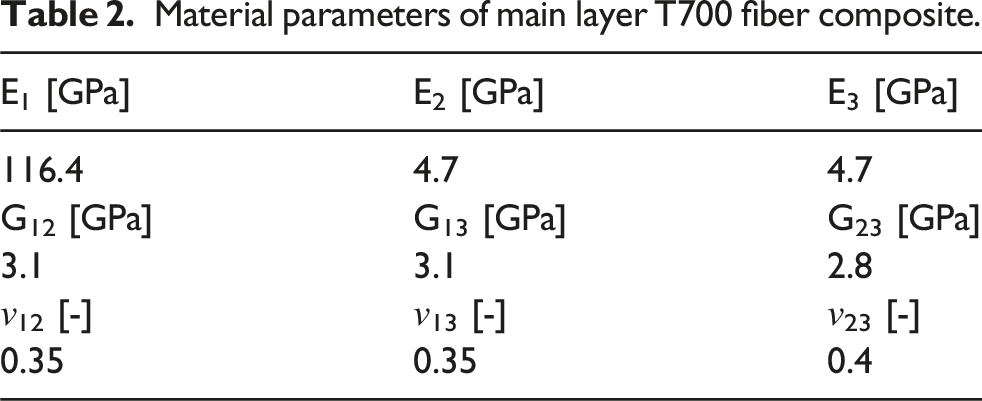
Material parameters of main layer T700 fiber composite.

E₁ [GPa]	E₂ [GPa]	E₃ [GPa]
116.4	4.7	4.7
G₁₂ [GPa]	G₁₃ [GPa]	G₂₃ [GPa]
3.1	3.1	2.8
ν₁₂ [-]	ν₁₃ [-]	ν₂₃ [-]
0.35	0.35	0.4

Table 3.

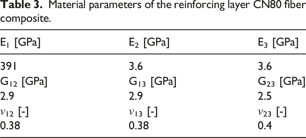
Material parameters of the reinforcing layer CN80 fiber composite.

E₁ [GPa]	E₂ [GPa]	E₃ [GPa]
391	3.6	3.6
G₁₂ [GPa]	G₁₃ [GPa]	G₂₃ [GPa]
2.9	2.9	2.5
ν₁₂ [-]	ν₁₃ [-]	ν₂₃ [-]
0.38	0.38	0.4

Analytical model

The analytical model should serve as a quick, undemanding, yet reliable tool for engineers when designing PFSJ based on load, dimensions, and other input parameters. The theory underneath is based on two assumptions.

First – the joint can be represented as a contact between two non-splined surfaces where the effect of splines is substituted by an increased friction coefficient between steel and composite. The argument for this assumption is that the tooth height is very low relative to the diameter D (for example, a few tenths of a millimeter on a diameter of around 50 mm), thus the number of teeth is high, resembling a very rough surface.

Second – the intrusion of teeth of the steel part into the composite part induces stress that can be modeled using the theory of thick-walled cylinders. This theory is well described in textbooks^35,36 and subsequently in modified forms.^37,38 It is worth mentioning that a simpler theory of shell cylinders was also considered and tried. But it was discarded as it neglects the stress in the thickness of the layers (radial stress), which is significant relative to other stress components due to the use of the 90° reinforcing layer. Therefore, the theory of shell cylinders produces too optimistic results.

Stress, pressure and load capacity

The stress analysis in the model is based on the following differential equation: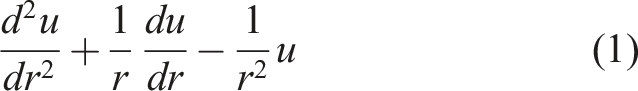

\frac{d^{2} u}{d r^{2}} + \frac{1}{r} \frac{d u}{d r} - \frac{1}{r^{2}} u

(1)

where r is radius, u is radial deformation (see Figure 4). And Hooke’s law: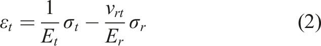

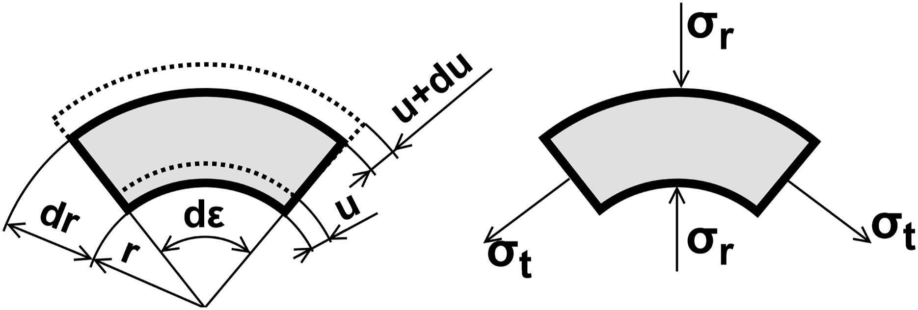
ε_{t} = \frac{1}{E_{t}} σ_{t} - \frac{ν_{r t}}{E_{r}} σ_{r}

(2)

Figure 4.

Infinitesimal element for equations (1)–(4). Dimensions and deformations (left) and stress (right).

where E is Young’s modulus, ɛ refers to strain, and σ is stress. The indices t and r refer to the tangential and radial direction of the cylinder.

After solving the Euler type differential equation (1) and combining with (2) according to Ref. 35,36 we can obtain two fundamental equations for open thick walled cylinders: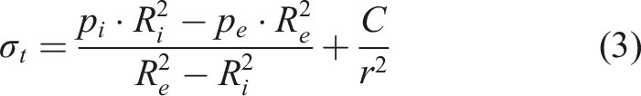

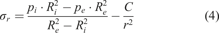
σ_{t} = \frac{p_{i} \cdot R_{i}^{2} - p_{e} \cdot R_{e}^{2}}{R_{e}^{2} - R_{i}^{2}} + \frac{C}{r^{2}}

(3)

σ_{r} = \frac{p_{i} \cdot R_{i}^{2} - p_{e} \cdot R_{e}^{2}}{R_{e}^{2} - R_{i}^{2}} - \frac{C}{r^{2}}

(4)

R_i and R_e are internal and external radii of the cylinder, and p_i and p_e are internal and external pressures. C is a constant that will be later eliminated, and r is a coordinate (current radius). E and ν are respective Young’s moduli and Poisson’s constants.

Equations (3) and (4) can be added, resulting in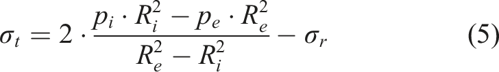

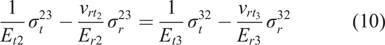
σ_{t} = 2 \cdot \frac{p_{i} \cdot R_{i}^{2} - p_{e} \cdot R_{e}^{2}}{R_{e}^{2} - R_{i}^{2}} - σ_{r}

(5)

The proposed PFSJ consists of four cylinders (shaft and three FRP layers), making the assembly statically indeterminate. For a complete determination, three deformation conditions are needed. Two of them are based on the assumption that the radii of two adjacent surfaces have the same change of radius after press-fitting. This results in equilibrium of the respective tangential strains ɛ_t(Δr/r = ɛ_t). That encompasses contact surfaces between layers 1 and 2 – equation (6), and between 2 and 3 – equation (7). The upper indices in (6), (7) and the following equations hereafter refer to the current layer and the layer that it is in contact with. For example, $ε_{t}^{12}$ refers to the tangential strain of layer 1 at the interface with layer 2, and $ε_{t}^{21}$ refers to tangential strain of layer 2 at the interface with layer 1.

ε_{t}^{12} = ε_{t}^{21}

(6)

ε_{t}^{23} = ε_{t}^{32}

(7)

The third deformation condition (8) is based on change of radii after press-fitting caused by interference δ between steel shaft and composite tube (layers 0 and 1). The scheme of this is in Figure 5. The strain $ε_{t}^{01}$ has a negative sign because the deformation is compressive. R₀₀ is radius of the steel shaft before deformation.

\frac{δ}{R_{00}} = ε_{t}^{10} - ε_{t}^{01}

(8)

Figure 5.

Change of radii by press-fitting.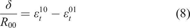

Now, all the three deformation conditions (6), (7) and (8) can be expressed using equation (2), which is an expression of tangential strain using Hooke’s law for orthotropic materials. The tangential and radial Young’s moduli are homogenized for the whole layer. R₀ in (11) was originally referred to as R₀₀ in Figure 5 but for simplicity and consistency with equations (14)–(16) now referred to as R₀.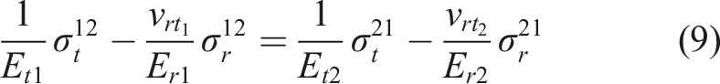

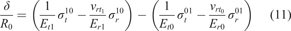
\frac{1}{E_{t 1}} σ_{t}^{12} - \frac{ν_{r t_{1}}}{E_{r 1}} σ_{r}^{12} = \frac{1}{E_{t 2}} σ_{t}^{21} - \frac{ν_{r t_{2}}}{E_{r 2}} σ_{r}^{21}

(9)

\frac{1}{E_{t 2}} σ_{t}^{23} - \frac{ν_{r t_{2}}}{E_{r 2}} σ_{r}^{23} = \frac{1}{E_{t 3}} σ_{t}^{32} - \frac{ν_{r t_{3}}}{E_{r 3}} σ_{r}^{32}

(10)

\frac{δ}{R_{0}} = (\frac{1}{E_{t 1}} σ_{t}^{10} - \frac{ν_{r t_{1}}}{E_{r 1}} σ_{r}^{10}) - (\frac{1}{E_{t 0}} σ_{t}^{01} - \frac{ν_{r t_{0}}}{E_{r 0}} σ_{r}^{01})

(11)

Equations (9)–(11) can be adjusted using equation (5) which expresses tangential stress as a function of pressures, radii, and radial stress. The external pressure on layer 3 is considered zero. In addition, the radial stress is equal to negative value of pressure (σ_r = −p). In the case of a solid steel shaft (without a hole), the radial stress equals the tangential stress $(σ_{t}^{01} = σ_{r}^{01} = - p_{01})$ , and the material is isotropic thus E_r = E_t = E.

After this and further adjustment, the problem can be expressed in matrix form 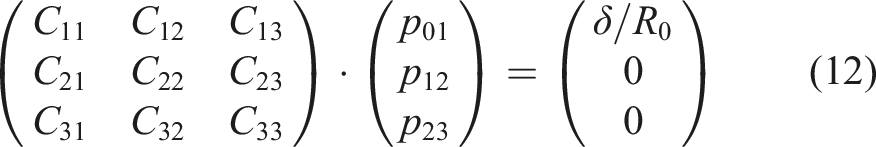C ⋅ p = δ . Where C is a matrix of material parameters and geometry, p is a vector of pressures between layers and δ is a vector that contains the interference in its first row.

(\begin{matrix} C_{11} & C_{12} & C_{13} \\ C_{21} & C_{22} & C_{23} \\ C_{31} & C_{32} & C_{33} \end{matrix}) \cdot (\begin{matrix} p_{01} \\ p_{12} \\ p_{23} \end{matrix}) = (\begin{matrix} δ / R_{0} \\ 0 \\ 0 \end{matrix})

(12)

Non-zero elements of the matrix C are the diagonal and one element adjacent to the diagonal (in this case elements C₁₃ and C₃₁ have value zero). As follows from the previous equations, for the i-th row of the matrix C the expressions for the non-zero elements are:

C_{i, i - 1} = - \frac{2 \cdot R_{(i)}^{2}}{E_{t_(i)} \cdot (R_{(i)}^{2} - R_{(i - 1)}^{2})}

(13)

\begin{aligned} C_{i, i} = \frac{2 \cdot R_{(i - 1)}^{2}}{E_{t_(i - 1)} \cdot (R_{(i - 1)}^{2} - R_{(i - 2)}^{2})} + \\ + \frac{2 \cdot R_{(i - 1)}^{2}}{E_{t_(i)} \cdot (R_{(i)}^{2} - R_{(i - 1)}^{2})} + \frac{ν_{r t_(i)}}{E_{r_(i)}} - \frac{ν_{r t_(i - 1)}}{E_{r_(i - 1)}} + \\ + \frac{1}{E_{t_(i)}} - \frac{1}{E_{t_(i - 1)}} \end{aligned}

(14)

C_{i, i + 1} = - \frac{2 \cdot R_{(i)}^{2}}{E_{t_(i)} \cdot (R_{(i)}^{2} - R_{(i - 1)}^{2})}

(15)

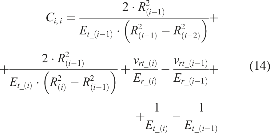
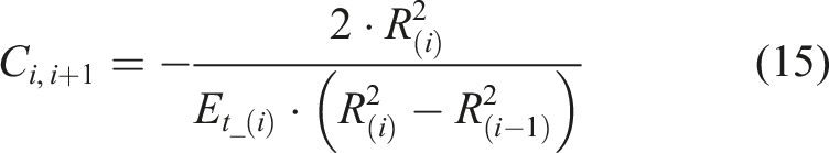
The output from the system of equations characterized by (12) is the vector of pressures between the individual layers. And it is the pressure p₀₁ that is used to calculate the load capacity of PFSJ T_max. Using equation (16), where L refers to the length of the joint and f is a friction coefficient between layers 0 and 1. The parameter f alongside with δ characterize the joint depend on the geometry of splines (height, angle, number of teeth) and must be determined experimentally.

T_{\max} = 2 π \cdot p_{01} \cdot R_{0}^{2} \cdot L \cdot f

(16)

Damage

The selected criterion for damage modeling is the Hashin damage criterion³⁹ due to its capability to account for stress in thickness (radial stress σ_r), which is crucial for modeling thick-walled cylinders. Other basic criteria consider only 2D plane stress. But in the model using thick-walled cylinders, the radial stress is a non-negligible component. For the purpose of completeness, the criteria for individual modes are listed in the following equations. X, Y and refer to strength in longitudinal and transversal direction, S is shear strength, the indices T and C refer to tension and compression and σ refer to stress with respective orientation to the coordinate system aligned with fiber direction.

Mode 1 - Fiber tension (σ₁₁ ≥ 0):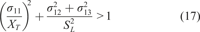

{(\frac{σ_{11}}{X_{T}})}^{2} + \frac{σ_{12}^{2} + σ_{13}^{2}}{S_{L}^{2}} > 1

(17)

Mode 2 - Fiber compression (σ₁₁ ≤ 0):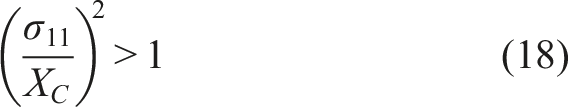

{(\frac{σ_{11}}{X_{C}})}^{2} > 1

(18)

Mode 3 - Matrix tension (σ₂₂ + σ₃₃ > 0):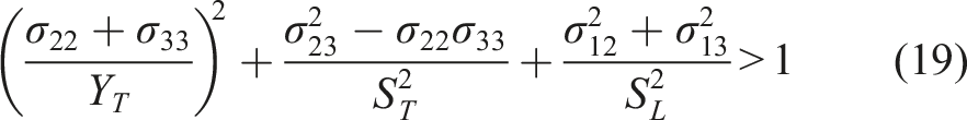

{(\frac{σ_{22} + σ_{33}}{Y_{T}})}^{2} + \frac{σ_{23}^{2} - σ_{22} σ_{33}}{S_{T}^{2}} + \frac{σ_{12}^{2} + σ_{13}^{2}}{S_{L}^{2}} > 1

(19)

Mode 4 - Matrix compression (σ₂₂ + σ₃₃ < 0):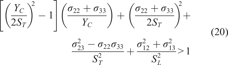

\begin{aligned} [{(\frac{Y_{C}}{2 S_{T}})}^{2} - 1] (\frac{σ_{22} + σ_{33}}{Y_{C}}) + {(\frac{σ_{22} + σ_{33}}{2 S_{T}})}^{2} + \\ \frac{σ_{23}^{2} - σ_{22} σ_{33}}{S_{T}^{2}} + \frac{σ_{12}^{2} + σ_{13}^{2}}{S_{L}^{2}} > 1 \end{aligned}

(20)

The damage of the GFRP layer (layer 1) is left out from the calculation of this criterion, because during the press-fitting the splined steel part itself can possibly induce damage such as fiber breakage and plasticity or even crack of the matrix. Modeling the stress and subsequent damage of this layer based on thick-walled cylinder theory that assumes smooth surfaces would be a misrepresentation of reality.

The damage of the reinforcing layer (layer 3) is calculated directly using the tangential and radial stresses calculated by the thick-walled cylinder theory, as the fibers are aligned with the coordinate system of the tube due to the 90° fiber orientation. Therefore, σ_t = σ₁₁, and σ_r = σ₃₃. There is no stress in the axial direction (σ_a = σ₂₂ = 0) nor any shear stress. The layer has two failure modes: mode 1 – Fiber tension and mode 4 – Matrix compression.

The damage of the main layer that transmits torque further to the driveline (layer 2) can’t be simplified in the same way as the reinforcing layer because it can theoretically have multiple sub-layers with different fiber orientations. While σ_r always equals σ₃₃, σ_t obtained from the analysis using thick-walled cylinders theory for homogenized layer has to be transformed to the coordinate system that is aligned with orientation of fibers and calculated for each sub-layer within layer 2. That results in obtaining stresses σ₁₁, σ₂₂, as well as shear stress σ₁₂. For this transformation, classical lamination theory (CLT)⁴⁰ was utilized as it is an effective, established tool that is already frequently implemented in many solvers, including in-house solvers of engineering companies.

This simplification can be done although so far the stress is considered 3D and CLT considers only plane stress. But in this case, CLT is used only for obtaining stresses in a single plane to which σ_r thus σ₃₃ is perpendicular, does not interact with the other stress components and is not affected by the transformation. The transformation to the respective directions could be realized in 3D stress state, but this simplification is preferred due to the above-mentioned fact that the already existing solver or a code for CLT can be implemented into the workflow without losing much accuracy, making it an effective approach.

So, the input to the CLT is the force in direction x of the laminate F_x (aligned with the tangential direction of the tube), which is calculated using the tangential stress σ_t, and possibly also the shear force F_x calculated using torsional stress caused by torque (see equation (21)). Moments M_x, M_y and M_xy are zero in case of sole torque load.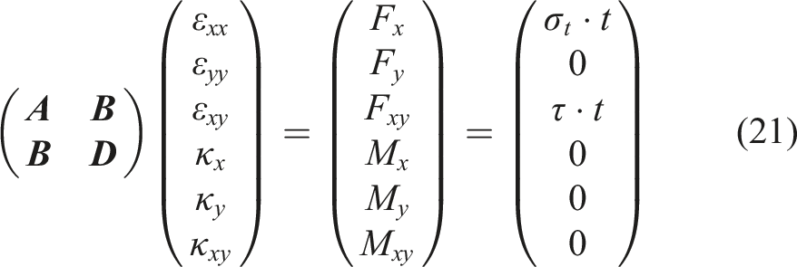

(\begin{matrix} A & B \\ B & D \end{matrix}) (\begin{matrix} ε_{x x} \\ ε_{y y} \\ ε_{x y} \\ κ_{x} \\ κ_{y} \\ κ_{x y} \end{matrix}) = (\begin{matrix} F_{x} \\ F_{y} \\ F_{x y} \\ M_{x} \\ M_{y} \\ M_{x y} \end{matrix}) = (\begin{matrix} σ_{t} \cdot t \\ 0 \\ τ \cdot t \\ 0 \\ 0 \\ 0 \end{matrix})

(21)

where A , B and D are sub-matrices of a matrix defined by CLT constituting stiffness of the laminate based on Young’s moduli, orientations and thicknesses of layers. t is thickness of the layer. The resulting strains ɛ and curvatures κ in the laminate direction are then used to calculate the respective stress components of each sub-layer of layer 2 using formula 22:

(\begin{matrix} σ_{x x} \\ σ_{y y} \\ σ_{x y} \end{matrix}) = T_{σ}^{- 1} C T_{ε} (\begin{matrix} ε_{x x} + h \cdot κ_{x} \\ ε_{y y} + h \cdot κ_{y} \\ ε_{x y} + h \cdot κ_{x y} \end{matrix})

(22)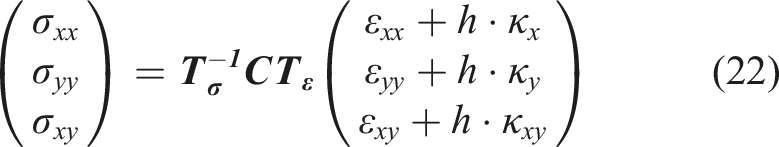

where h is the thickness of a sublayer, 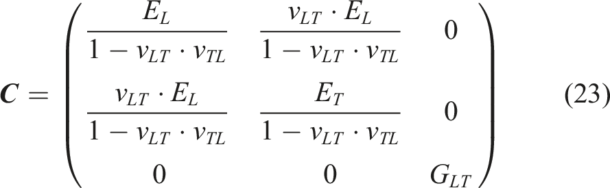T _ɛ and T _σ are the transformation matrices of stress and strain between above mentioned coordinate systems in respective sub-layers, and C is a stiffness matrix of a layer in the coordinate system aligned with the orientation of the fibers. The stiffness matrix equals to

C = (\begin{matrix} \frac{E_{L}}{1 - ν_{L T} \cdot ν_{T L}} & \frac{ν_{L T} \cdot E_{L}}{1 - ν_{L T} \cdot ν_{T L}} & 0 \\ \frac{ν_{L T} \cdot E_{L}}{1 - ν_{L T} \cdot ν_{T L}} & \frac{E_{T}}{1 - ν_{L T} \cdot ν_{T L}} & 0 \\ 0 & 0 & G_{L T} \end{matrix})

(23)

The transformation matrices are then of the form written in equations (24) and (25) For shortening, sin(α) ≡ s(α) and cos(α) ≡ c(α)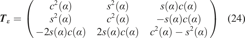

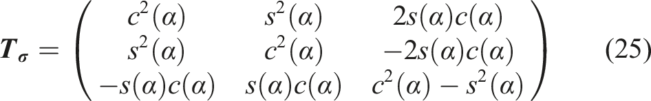
T_{ε} = (\begin{matrix} c^{2} (α) & s^{2} (α) & s (α) c (α) \\ s^{2} (α) & c^{2} (α) & - s (α) c (α) \\ - 2 s (α) c (α) & 2 s (α) c (α) & c^{2} (α) - s^{2} (α) \end{matrix})

(24)

T_{σ} = (\begin{matrix} c^{2} (α) & s^{2} (α) & 2 s (α) c (α) \\ s^{2} (α) & c^{2} (α) & - 2 s (α) c (α) \\ - s (α) c (α) & s (α) c (α) & c^{2} (α) - s^{2} (α) \end{matrix})

(25)

After obtaining the stress components in the coordinate system of the laminate, the last step is the transformation to the coordinate system aligned with fiber direction. Then these resulting stress components are, along with the radial stress, the inputs to the damage calculation stated in equations (17)–(20).

(\begin{matrix} σ_{11} \\ σ_{22} \\ σ_{12} \end{matrix}) = T_{σ} (\begin{matrix} σ_{x x} \\ σ_{y y} \\ σ_{x y} \end{matrix})

(26)

Behavior of the joint according to the analytical model

The analytical model allows exploring the influence of key parameters on the load bearing capacity of the joint. While the influence of length of the joint and the friction coefficient are simply proportional, other parameters such as central diameter of the shaft D₀ (diameter to radius R₀), interference δ, and thicknesses of the layers, together with material and technological limitations, play a crucial role in determining the torque that the joint can transfer.

Figure 6 shows the maximal transferable torque at given diameter D₀ and different interference δ values. This calculation takes into account material parameters, including limit stresses. Another limitation is technological. The thickness of either the main layer or the reinforcing layer should be within certain limits. The minimal thickness of the main layer was set to 1 mm so that it could be manufactured by filament winding and the tube does not undergo buckling. The minimal thickness of the reinforcing layer was 0.5 mm and maximal thickness 5 mm solely for manufacturing purposes. The value 5 mm can be debatable, depends on many factors, and may be set even higher. The last important choice was to set the thickness of the main layer so that the safety coefficient with respect to the torque load of the tube is equal to 2 which helps to compensate edge effects at the end of the joint, and ensures that the weakest link is the joint. These practical limitations help to keep the results meaningful not only mathematically but also for real-world applications. The friction coefficient was set at 0.4 and the length of the joint at 25 mm.

Figure 6.

Influence of the shaft diameter and the interference δ (varying from 0.02 mm to 0.1 mm) on load bearing capacity.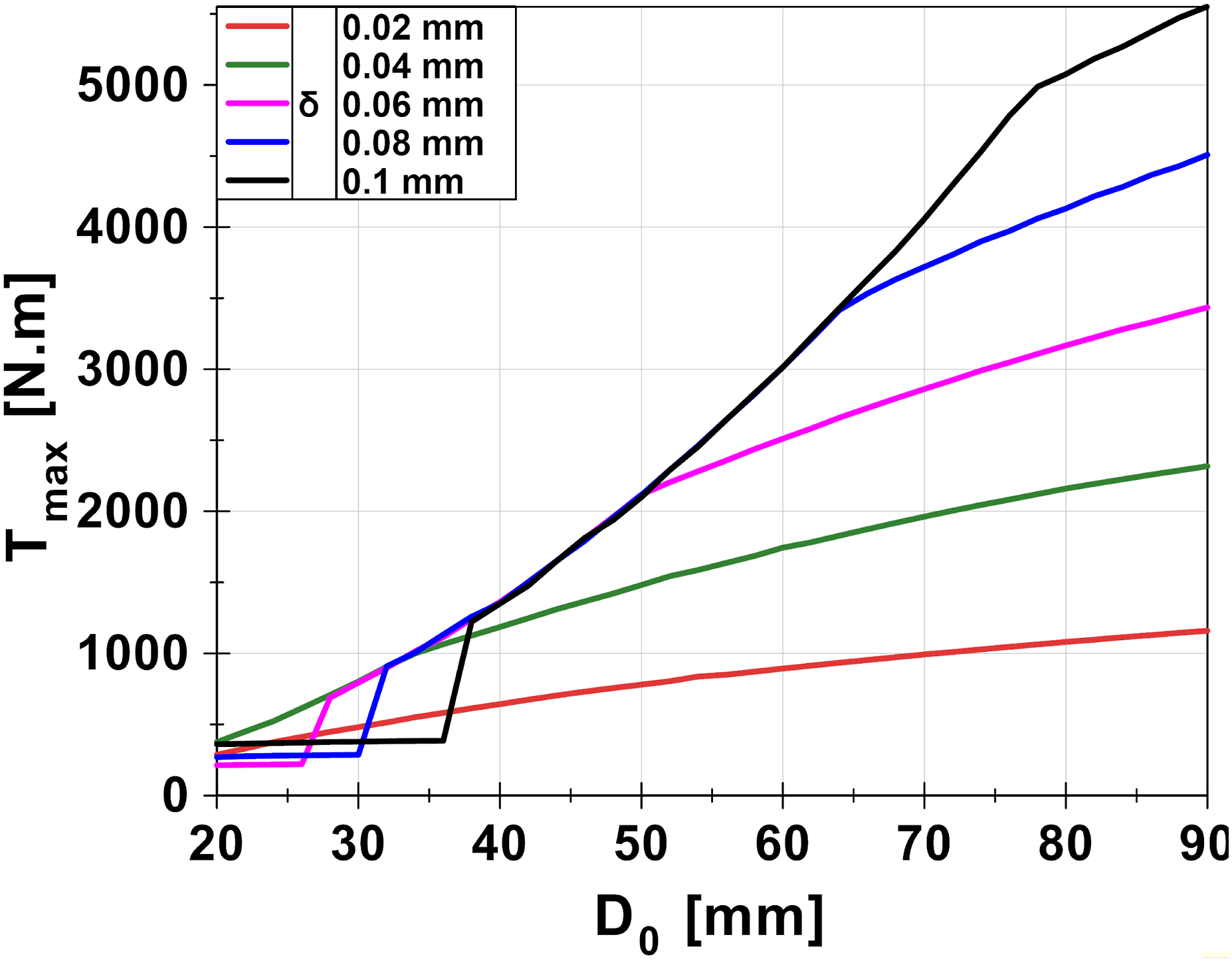

Figure 7 then provides insight into how the thicknesses of layers were set to achieve the maximal load bearing capacity at a given diameter D₀ and interference δ, while honoring the limitations. The graph offers several takeaways. The first one is that for higher values of interference and small diameters, it is not possible to have any reinforcing layer as it would create too much stress in the joint or in the reinforcing layer itself. The second one is that as the diameter increases, the thickness of the reinforcing layer has to increase too in order to achieve maximum load bearing capacity. And the third one, that when the thickness of the reinforcing layer reaches its limit, the thickness of the main layer needs to decrease with increasing diameter D₀ to compensate the loss of internal pressure in the joint with increasing diameter and stable reinforcement layer.

Figure 7.

Thicknesses of layers at given diameter and interference δ (varying from 0.02 mm to 0.1 mm).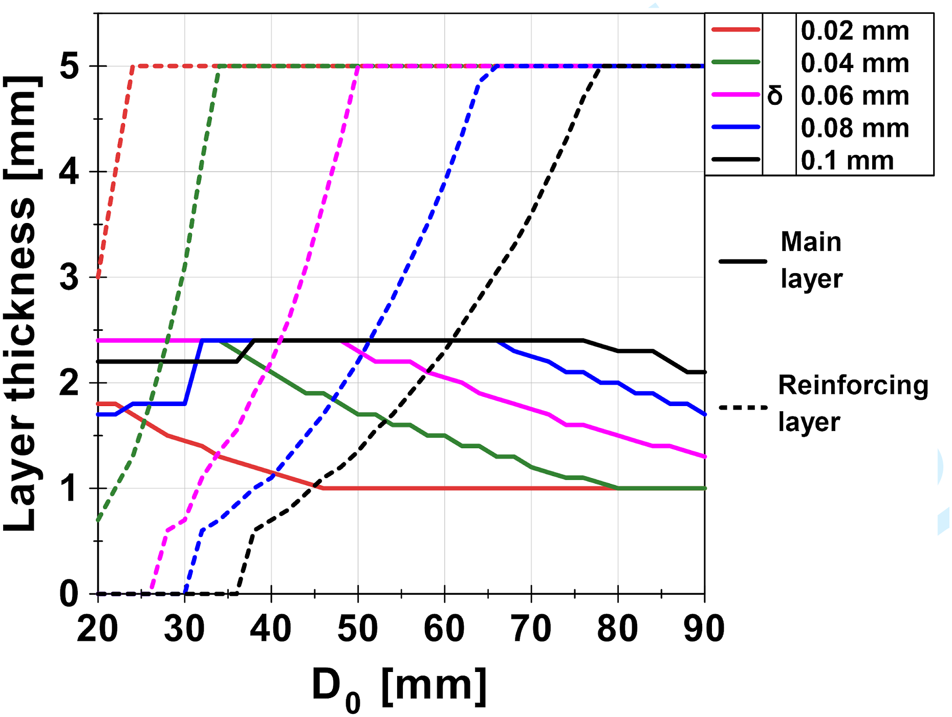

Figure 8 does not show the maximal achievable load bearing capacity as Figure 6 does, but it shows the trends how thickness of the main layer and the reinforcing layer influences the load bearing capacity. For this example, a single case was chosen where δ = 0.08, D₀ = 50 mm, the friction coefficient and the joint length remained the same as in the previous case. The load bearing capacity is proportional to the values of the friction coefficient and the length of the joint, so the results can be scaled up or down depending on the choice of these parameters. This calculation also honored the material limits, but did not keep the safety factor 2. The trend is clear that for the constant value of the reinforcing layer, decreasing the thickness of the main layer increases the torque and vice versa.

Figure 8.

Load bearing capacity depending on the reinforcing layer thickness (x-axis) at different main layer thickness (lines) while δ = 0.08 mm and D₀ = 50 mm.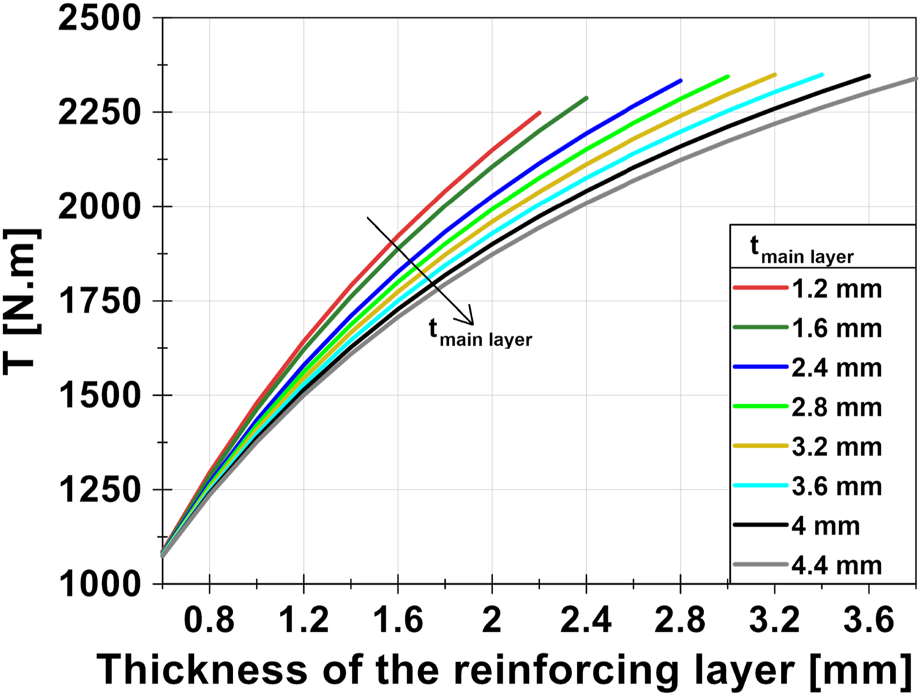

Verification of the analytical model using finite element method

This is the first of 3 chapters where the finite element method is used to improve understanding of the joint. The software used for the analysis was Abaqus 2019. All FEM models use 3D solid elements (C3D8R: An 8-node linear brick, reduced integration, hourglass control), because the continuum shell elements had a poor correlation of the results with both solid elements and the analytical model described in the previous section.

The objective in this section is to verify the correct functionality of the analytical model by using an FEM model with the same material parameters and geometry. The model represents the joint as a contact of two smooth surfaces loaded by geometric overclosure between steel and composite simulating the press-fitting, which is the same principle upon which the analytical model is built. Also, the friction behavior is added to the contact to be consistent with the analytical model. As previously stated, linear 3D solid elements were used not to exclude stress in the thickness of composite tubes, in contrast to the continuum shell elements that are usually used. Linear elastic orthotropic material was used to define mechanical properties that are identical to those of the analytical model.

The diameter of the shaft was chosen to be 52.2 mm, the tube inner diameter was 52 mm, the thickness of the glass fiber layer was 1.5 mm, thickness of the main layer was 4.4 mm and thickness of the reinforcing layer was 2 mm. The length of the joint as well as the reinforcing layer length was 20 mm. Length of the whole tube was 90 mm. The boundary conditions removing all degrees of freedom were applied to the section of the shaft that is outside the joint and to the end of the tube. The orientations were assigned to the composite layers (Glass fiber layer: 90°; Main layer: ±45° symmetric; Reinforcing layer 90°). The mesh, as mentioned above, consisted of C3D8R 3D stress elements with element length 0.7 mm and less at the joint and its nearest proximity, and 4 mm at the rest of the tube (Figure 9).

Figure 9.

FEM used model for verification.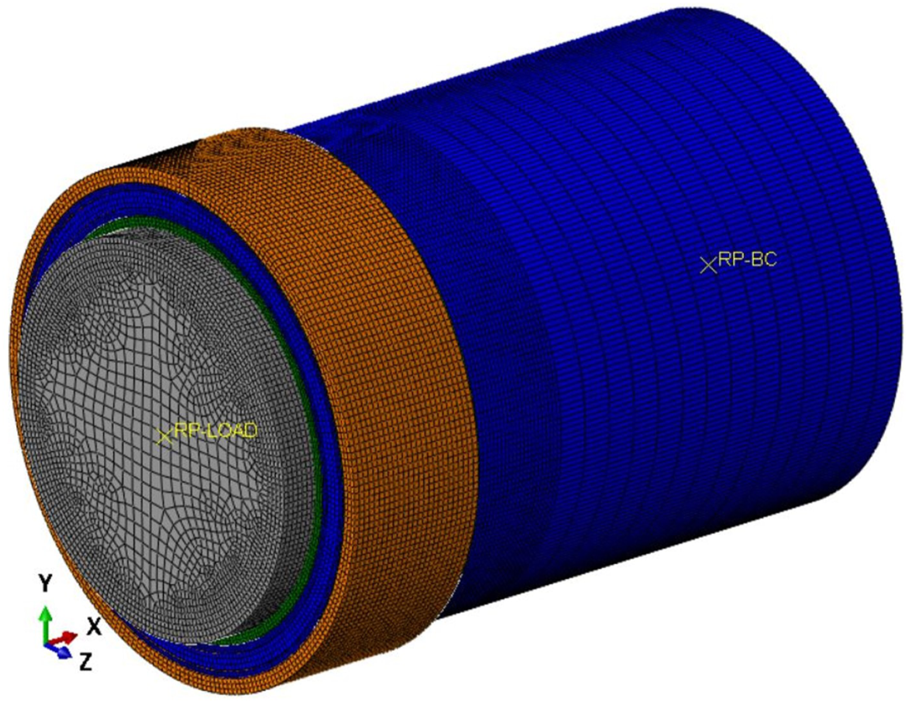

The individual parts are in contact with one another. The contact between the steel shaft and Layer 1 has two properties: Tangential behavior with friction coefficient 1 (the same as in the analytical model) and normal behavior defined by hard contact. These two parts differ in radius by 0.1 mm mm which induces a load in the joint when the contact is active. This is the equivalent of the parameter δ in the analytical model. The contact is then set to have surface-to-surface discretization method, finite sliding formulation, and no allowable interference with no adjustment of slave nodes.

For better visualization and readability of the data, as well as for better comparison of both analytical and FEM models, the data are processed in a form of graphs where the values are sorted by the x-coordinate that hereinafter has origin at the end of the steel shaft (see direction and origin in Figure 10) and averaged at respective x-coordinate and radius.

Figure 10.

x-coordinate, origin and direction.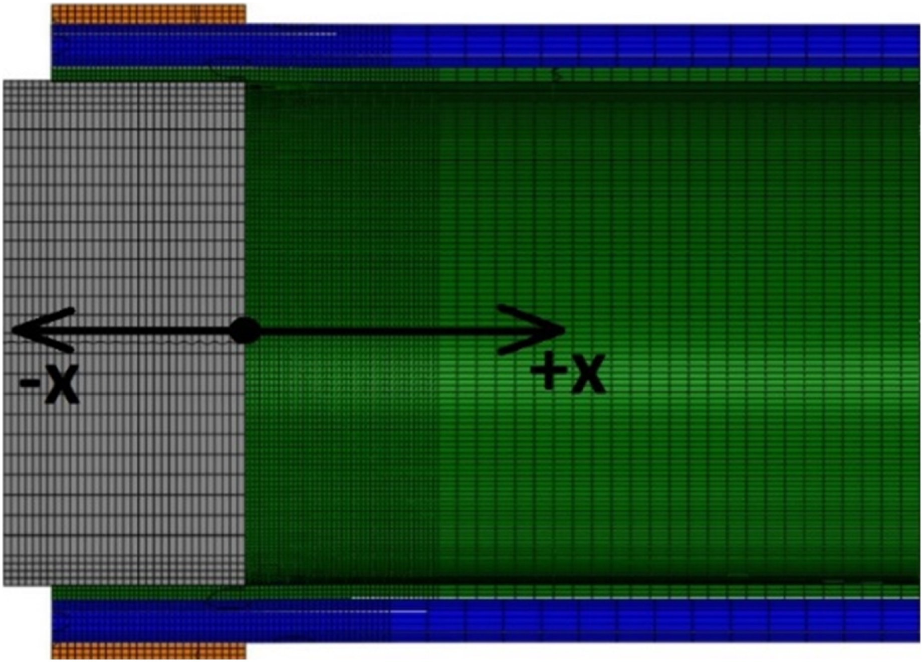

The relevant results and comparison with the analytical model are shown in the following figures (Figure 11–14). Each dashed line refers to the value in the analytical model, and the solid line refers to the average value at coordinate x of the FEM model (results from elements or nodes on the same circumference were averaged). Figure 15 compares radial and tangential stresses obtained from the FEM model (averaged at a given radius) and the analytical model using equations (3) and (4).

Figure 11.

Comparison: p₀₁.

Figure 12.

Comparison: layer 2 Hashin damage - mode 4.

Figure 13.

Comparison: layer 3 Hashin damage - mode 1.

Figure 14.

Comparison: layer 3 Hashin damage - mode 4.

Figure 15.

Comparison of stress curves in PFSJ.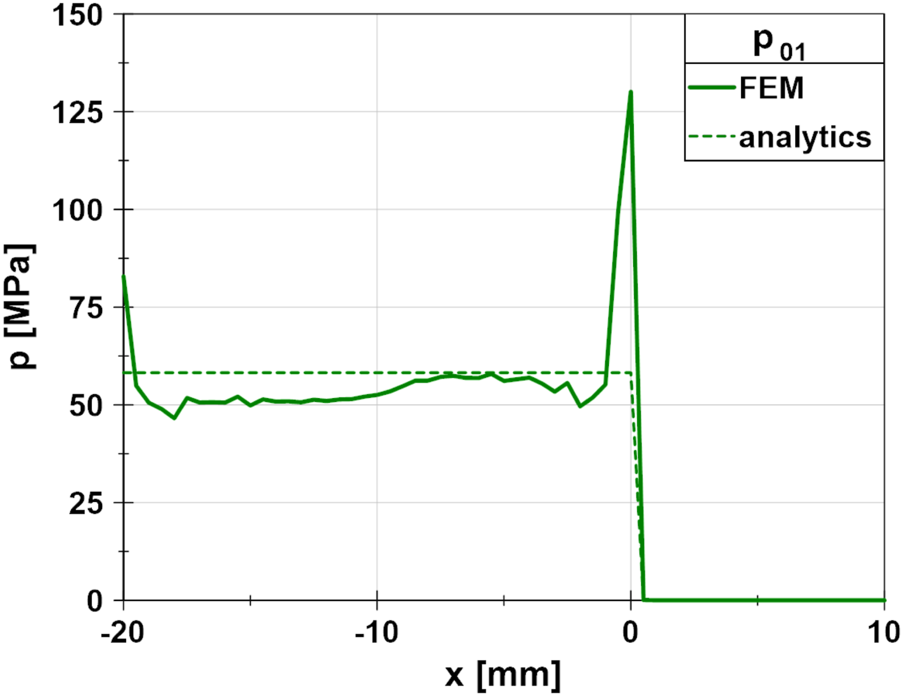

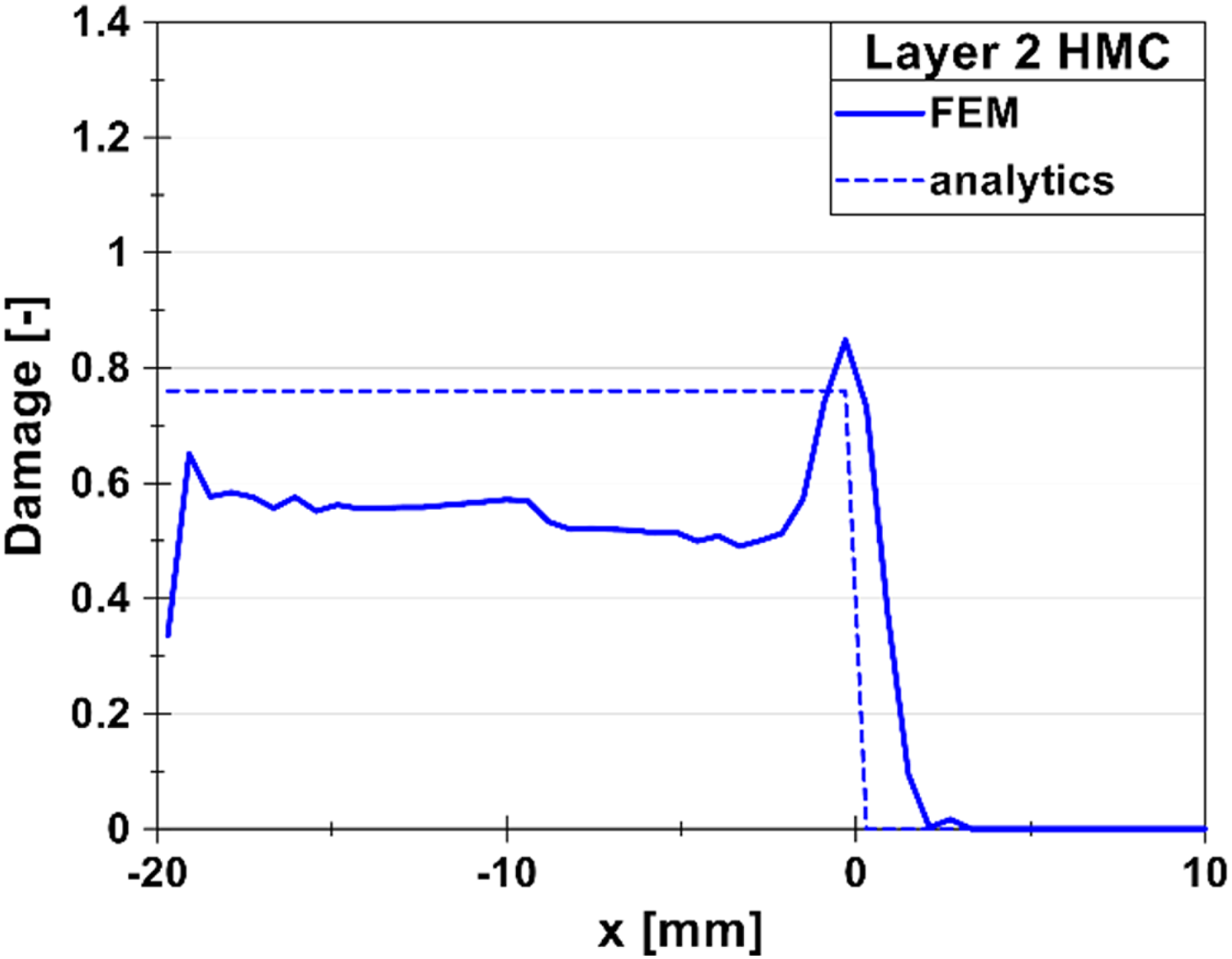
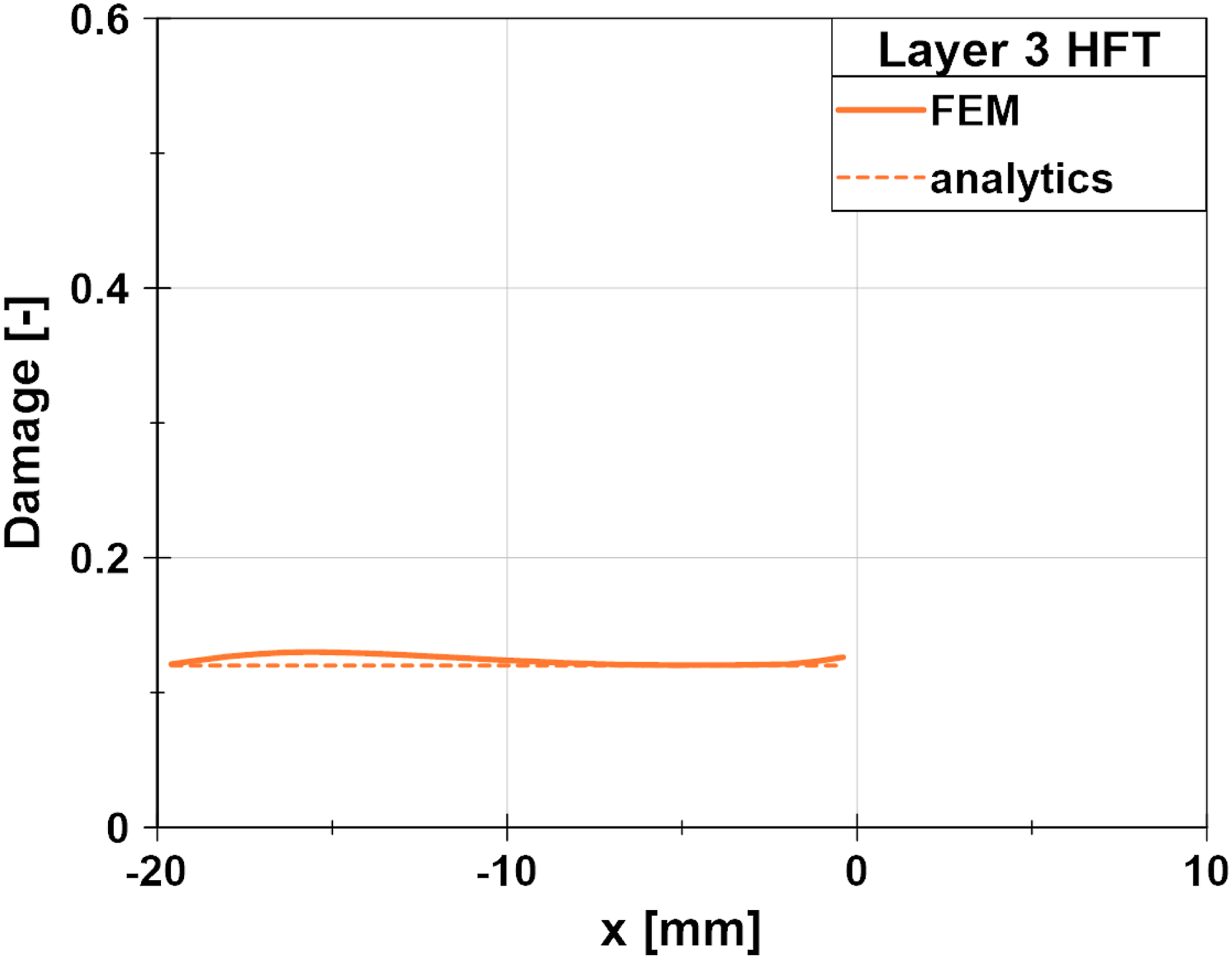
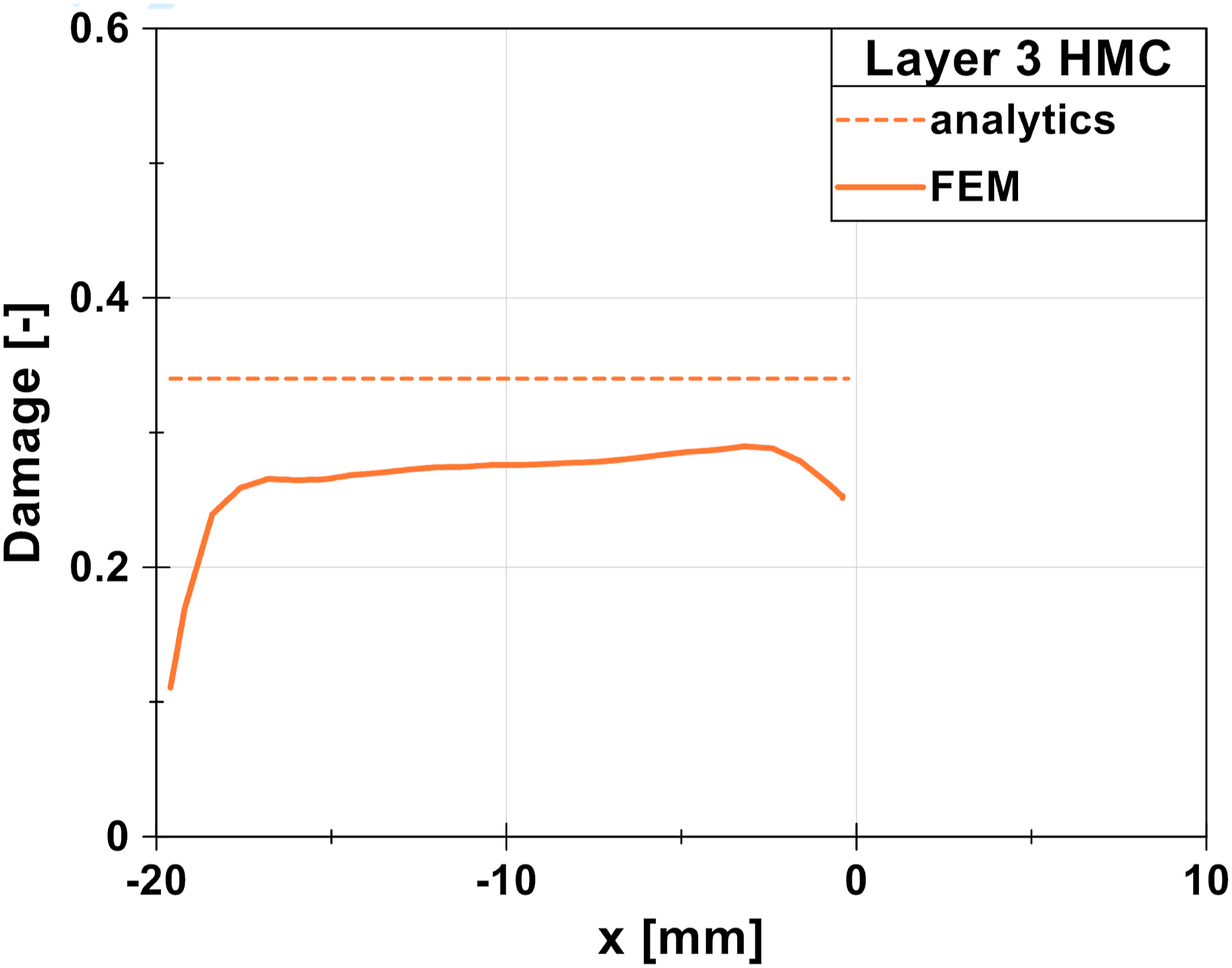
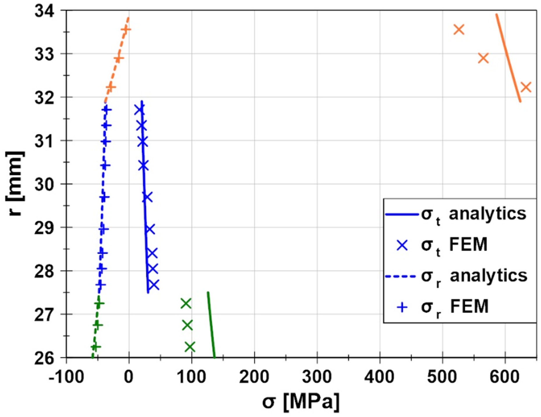
The FEM model of PFSJ showed good correlation with the analytical model over most of the length of the PFSJ and proved it viable for further use. The main differences in the results are caused by discretization of the FEM model, where for example σ_r is evaluated in integration points and not directly at the interface with previous layer as it is the case in the analytical model. Other divergences will be discussed and analyzed in the next section.

Reinforcing layer study

The previous results in Figure 11 and 12 show a sudden increase in pressure and stress at coordinate x = 0. This peak is caused by a change in geometry as the steel shaft is ended, creating de facto a notch. This edge effect is not taken into account in the analytical model except for a sufficiently high safety factor. The question is what the influence of the length of the reinforcing layer (Layer 3) on this peak is. Could a longer reinforcing layer flatten the peak? What happens when the reinforcing layer is shorter? To answer these questions, several variants of the same FEM model described in the previous section were made varying the length of the reinforcing layer starting at 5 mm shorter than the original one and ending 5 mm longer with a step of 1 mm, making it a total of 11 variants (Figure 16–19).

Figure 16.

p₀₁ depending on overlap.

Figure 17.

Layer 2 Hashin damage mode 4.

Figure 18.

Layer 3 Hashin damage mode 1.

Figure 19.

Layer 3 Hashin damage mode 4.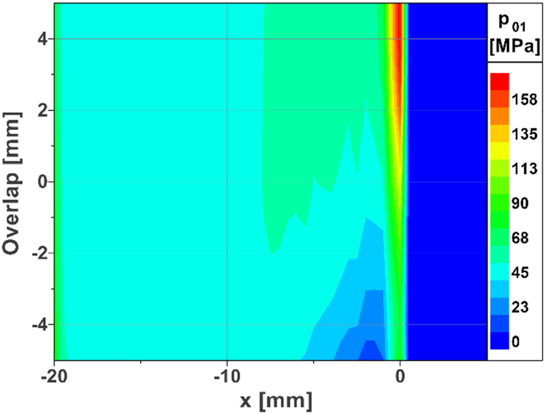

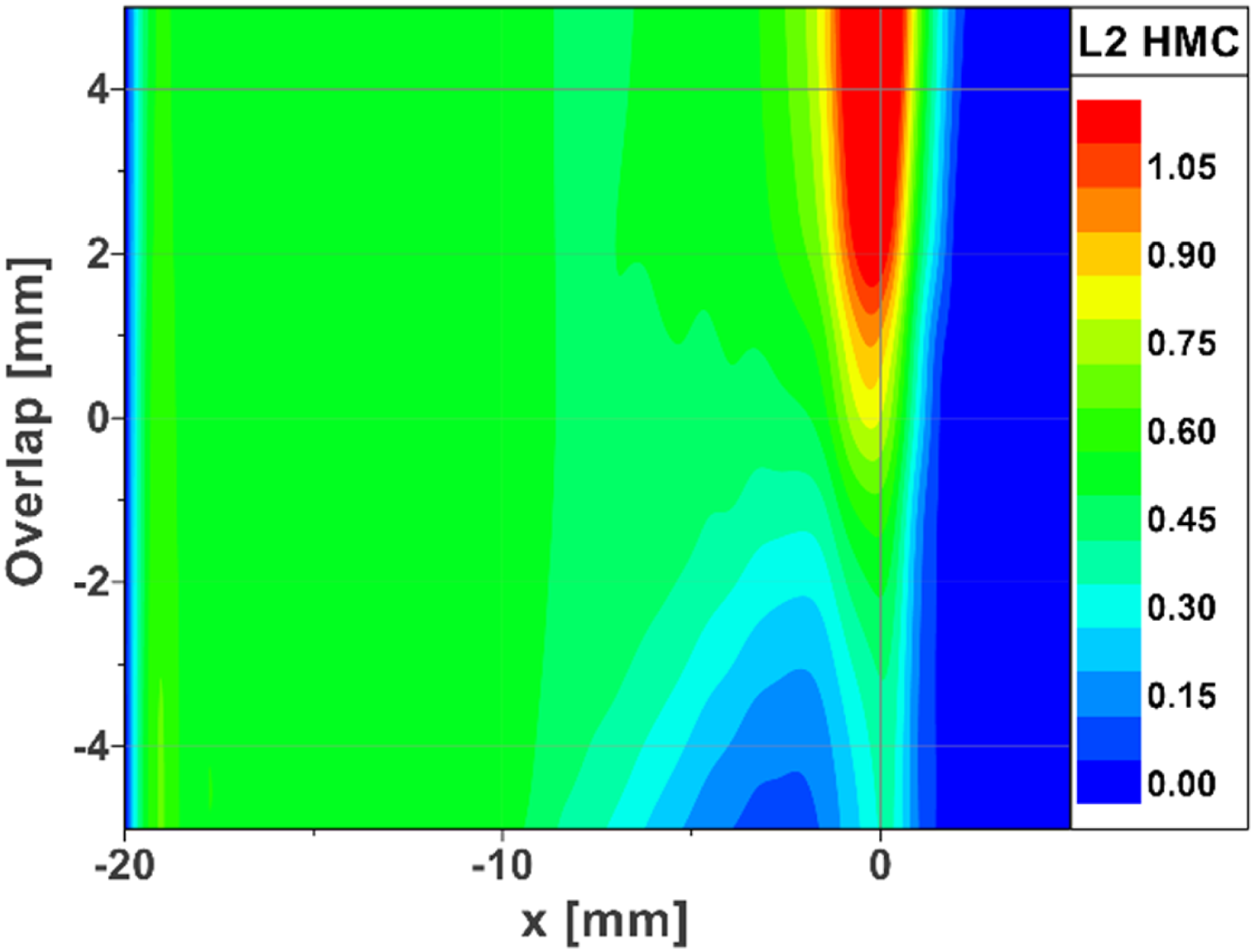
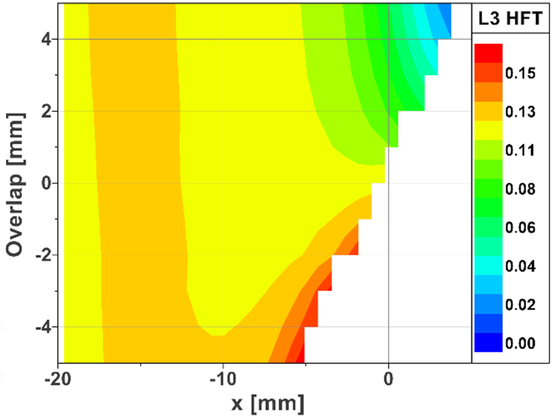
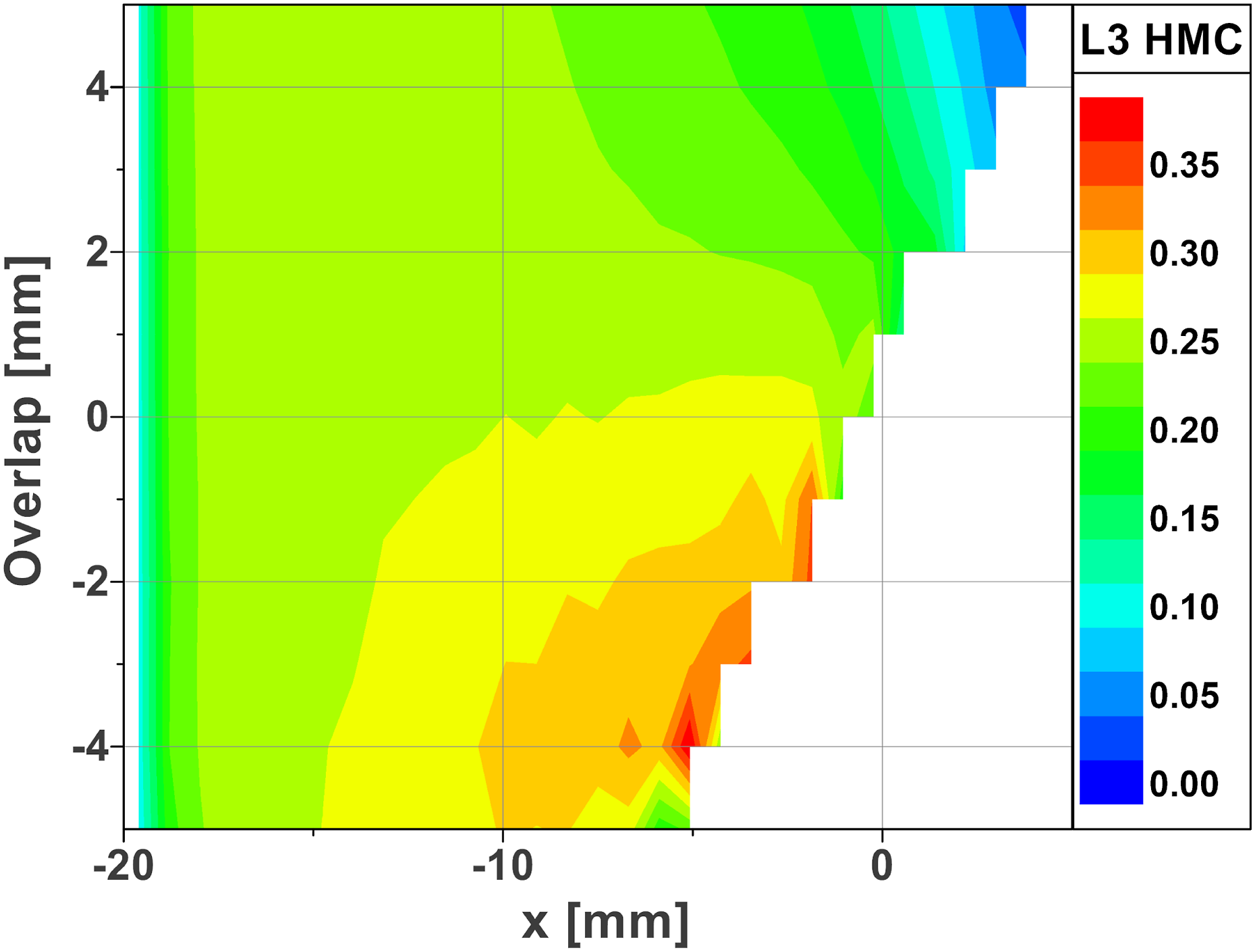
The variants in the graphs are distinguished by the parameter ’overlap’ that varies from −5 mm to +5 mm. It means that if the reinforcing layer is for example 3 mm shorter than the original one (ending at x coordinate −3 mm), the parameter ’overlap’ equals −3 mm. The following graphs show the pressure p₀₁ and relevant damage parameters in the form of a contour graph, as 2D graphs tend to be not clear enough to distinguish individual variants.

Several trends can be observed in the results. The pressure p₀₁ increases rapidly at x = 0 when the overlap is greater than 0 mm. Also, damage (mode 4 - matrix compression) of layer 2 is highly sensitive to the length of the reinforcing layer at x = 0. The peak of the damage can be almost flattened with an overlap of −1 mm. The trend is opposite in layer 3. The longer the layer, the less damage is inflicted upon it. It is a compromise between maintaining a sufficiently high pressure p₀₁ (between steel and composite) on the one hand and not reaching critical damage. The solution and the recommendation for engineers seem to lie in maintaining the overlap in the range between 0 mm and −1 mm.

Teeth geometry

This set of FEM models was created to have a comparative analysis of various geometries of the teeth, and to know how tooth height (intrusion into the composite) and the angle of the teeth influences the load capacity of PFSJ.

This model with central diameter D 50 mm is based on the previous models, hence the composite tube layers have the same thickness as in the previous models and consist of 3D stress elements with orthotropic elastic behavior in respective orientations (glass and reinforcing layer - 90°, main layer ±45°). The material of the steel shaft is an elasto-plastic material; however, the yield stress is not reached in the simulation. A section of the steel shaft and the glass fiber layer is modeled in detail, including the geometry of the teeth and grove. These sections are then repeated five times in the assembly (see Figure 20). These sections are tied to the respective parts, that are modeled as simple smooth surfaces. The interaction between teeth and grooves is simulated by using contact with normal and tangential behavior.

Figure 20.

Model with detailed geometry of teeth.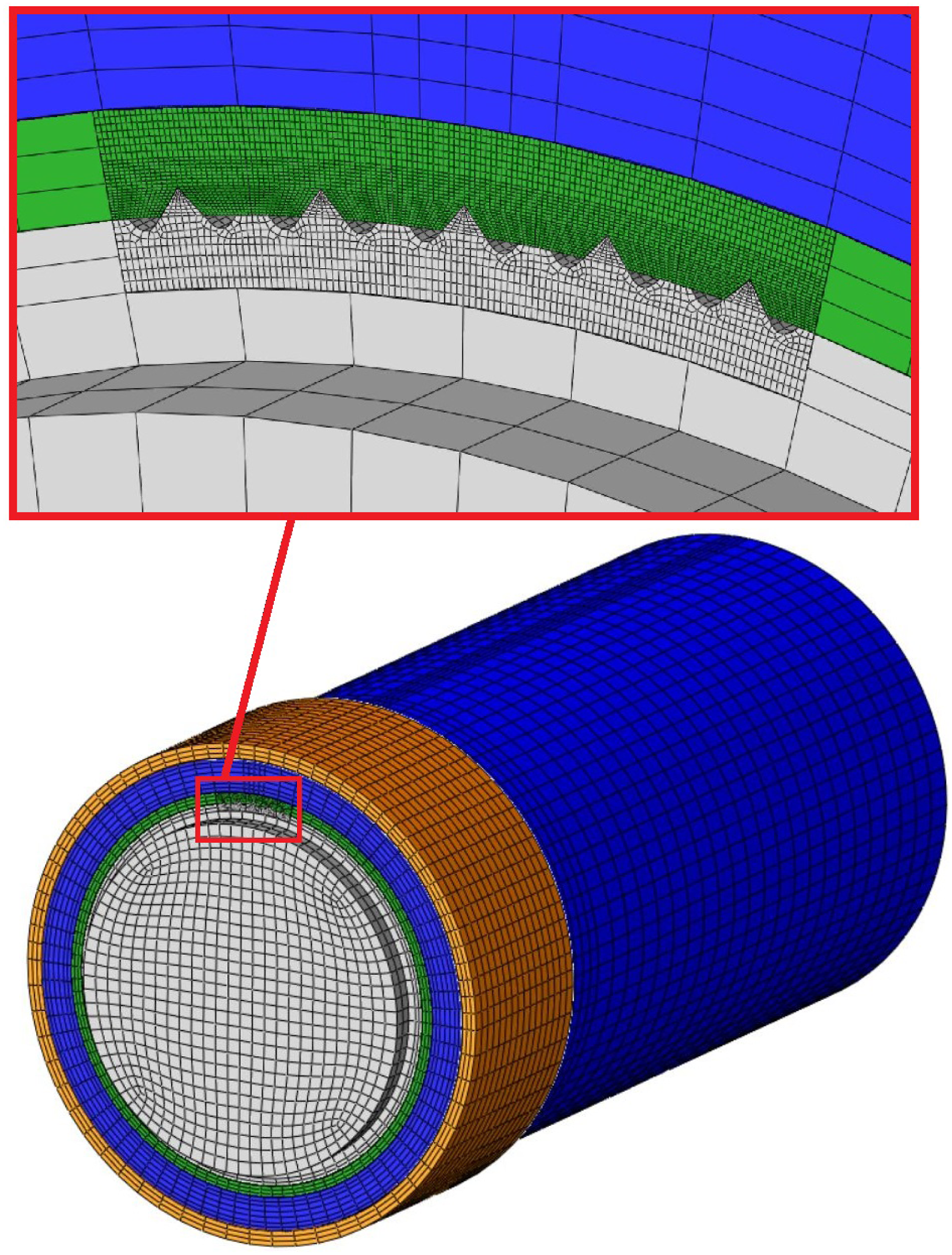

The loading process consists of two steps. Initially, an overclosure between the reinforcing layer (orange) and the main layer (blue) was added to induce stress in the joint, to create the same effect as the press-fitting. This overclosure is resolved in this first step. The overclosure value varies depending on tooth height. To determine the value, the analytical model and the results from the experiment (to be introduced in the following chapter) were used to induce an equivalent tangential stress on the outer diameter of the reinforcing layer. In a subsequent step, the torque with a maximum value equivalent to 7200 Nm is gradually applied to the shaft. However, since each variant features a different number of teeth, the torque value is adjusted accordingly.

The number of teeth that are modeled in detail was determined using the trial-and-error approach. It turned out that with five teeth, the influence of boundary effect (caused by tie constraint with smooth tube) on the middle tooth is negligible. The middle tooth is the only one relevant for further stress and damage analysis that is presented later in this chapter.

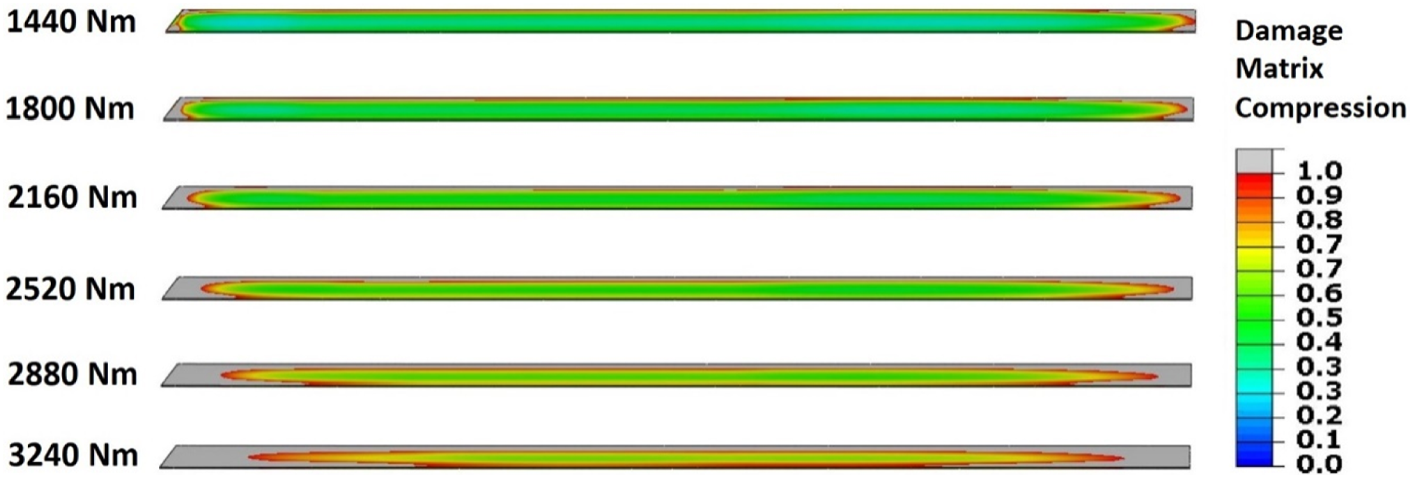
Figures 21 and 22 display an example of results. As previously, Hashin damage fields were created to analyze the maximum load of PFSJ. The most critical damage initiation mode was observed to be mode 4 – matrix compression. Figure 22 shows damage initiation progress of groove side with increasing load. The left side is the end of the groove (is tapered).

Figure 21.

Example of result - front view, Hashin damage mode 4 – matrix compression.

Figure 22.

Example of result - damage initiation of side of groove (Hashin damage mode 4 - matrix compression).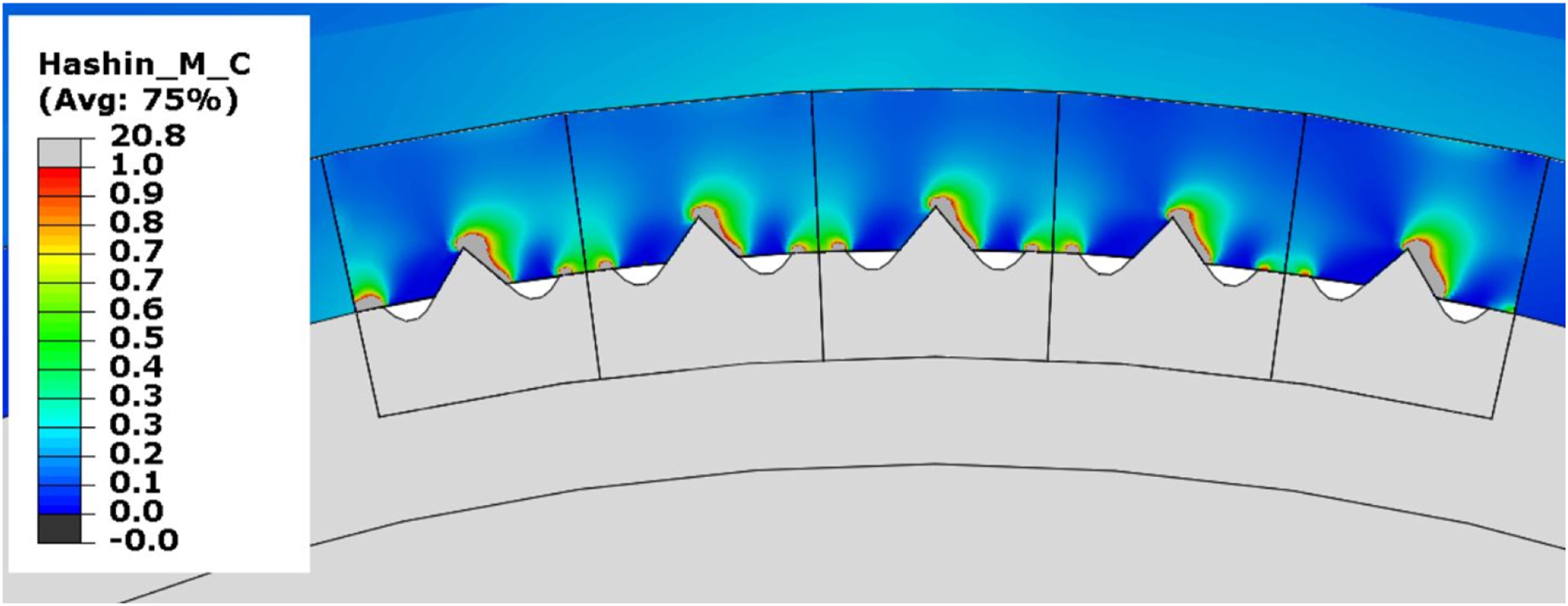

The analysis showed that sharper teeth have a better performance in transmitting the load. This is in part due to the fact that more teeth can fit on the circumference of the shaft resulting in a larger contact surface. But the maximal load per tooth is also bigger when using sharper teeth. Higher teeth contributed to increased load capacity, albeit with the caveat of potentially greater damage initiation during press-fitting, an aspect not addressed in great detail in the model. See the results for individual variants in Table 4. The maximum load was evaluated from the moment the damage initiation parameter exceeded the value 1 along the entire length of the groove side.

Table 4.

Maximal torque for each variant.

Max torque [Nm]		Tooth height h_t [mm]
		0.4	0.6	0.8
Tooth angle α_t	60°	3600	5040	5400
	80°	2520	3960	4680

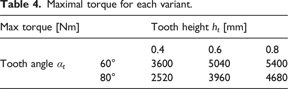
The best variant for PFSJ would be using teeth with 60° angle and 0.6 mm height, as 0.8 mm could be too risky in terms of press-fitting damage. The variant chosen for the experiment in the following chapter was 0.4 mm/ 80° and the results were correlated with the FEM model with the difference 16%. The difference might be attributed to smaller teeth (since in reality the tips are worn off) or to larger damage induced during press-fitting that was not entirely captured in the FEM model. In either case, the purpose of the model with the teeth geometry was first and foremost a comparison between individual variants rather than absolute precision, so this correlation is considered satisfactory.

Torque–twist response: experiment and simulation

The experiment was carried out on 300 mm long tubes with an inner diameter of 50 mm, 1 mm thick glass fiber layer, 4.4 mm thick layer of high strength fibers (T700) composite oriented at ± 45° symmetrically (main layer) and lastly the reinforcement layer of UHM fibers (CN80) composite was 3.5 mm thick. The steel shafts had splines with 0.4 mm tooth height and 80° tooth angle. The joint length was 25 mm as well as the length of the reinforcing layer length. The joints were on both ends of the test sample. The composite tubes were manufactured using filament winding technology.

While having no practical experience with this joint, the choice of the parameters of the test sample both tube dimensions and teeth geometry relied on models mentioned above, and to be fully transparent on engineering guess. The approach was fairly conservative; therefore, the thickness of the main layer was set, so the safety coefficient for the tube torsion was equal to 4, ensuring that the weakest part is the joint, not the tube. The same caution led to choice of teeth parameters so the tooth height was rather smaller not to induce too much damage by the press-fitting. The reinforcing layer was designed to increase the pressure in the joint to reach a torque level around 2500 Nm, large enough to be above 20% of torque sensor’s range, and low enough not to get close to tube strength. For this, interference δ and friction coefficient f (analytical model parameters) were estimated in advance at 0.06 mm and 0.6. The real values will be obtained from the experiment.

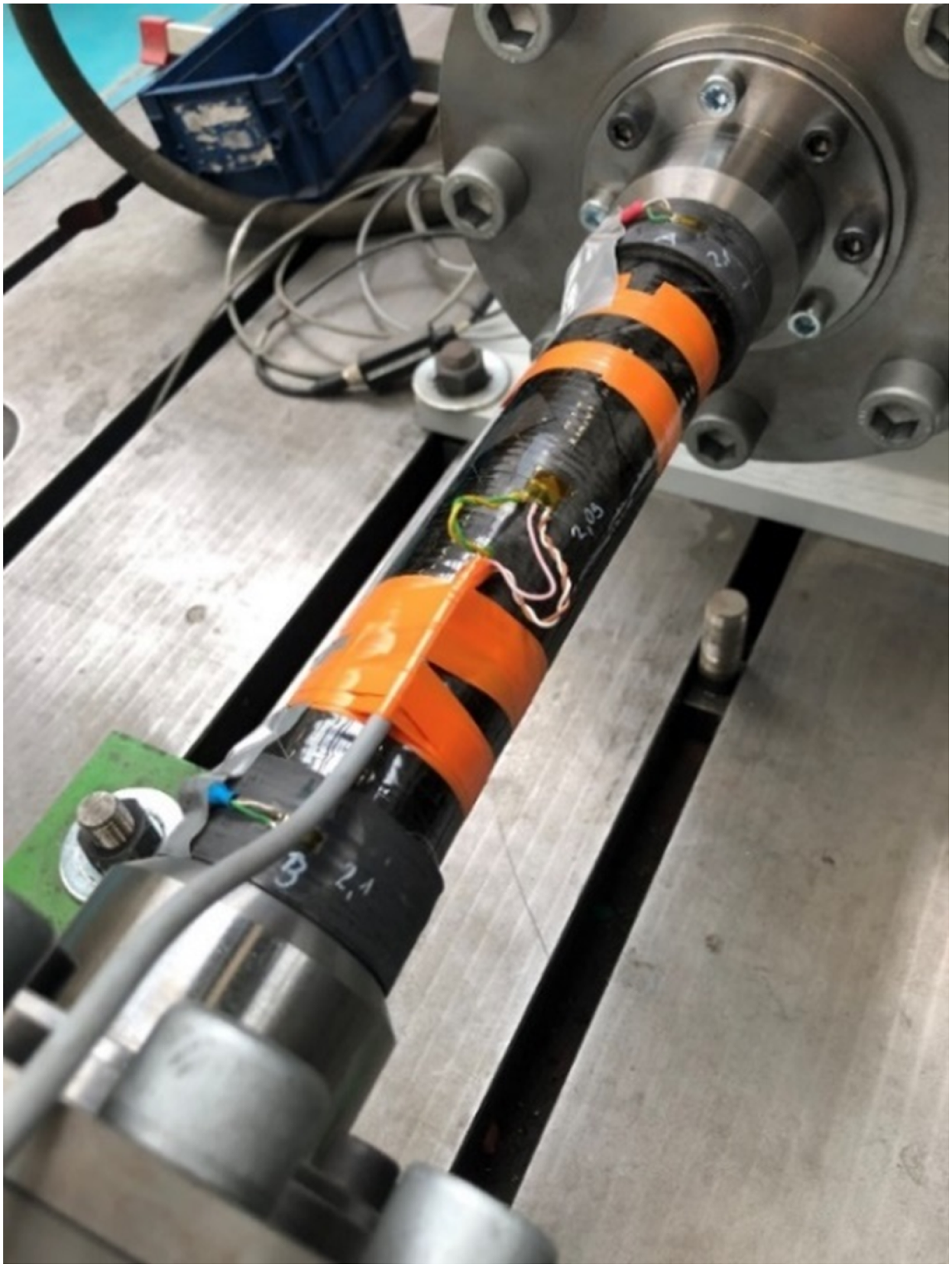
The test stand for the static torsion test consisted of several components. A hydraulic torsional actuator capable to generate torque up to 10 000 Nm. A torsionally stiff backlash-free coupling BK1-10,000. And torque sensor MF-8000 with nominal torque of 8000 Nm (Figures 23–24).

Figure 23.

Scheme of the test stand (cut section of test sample).

Figure 24.

Static torsion test.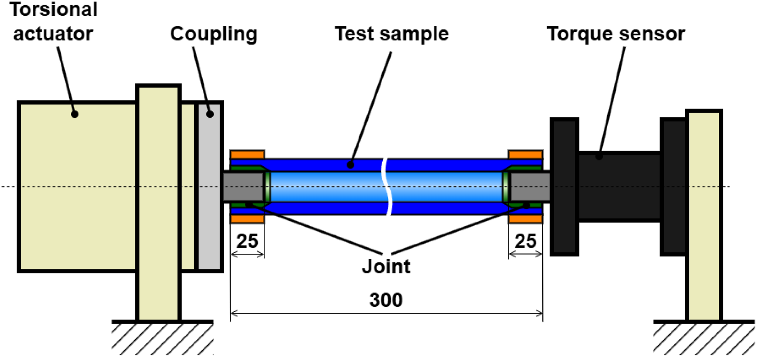

Also, the tangential strain on the outer surface of the reinforcing layer was measured during the press-fitting process to obtain the tangential stress from which the value of interference δ for the analytical model was deduced.

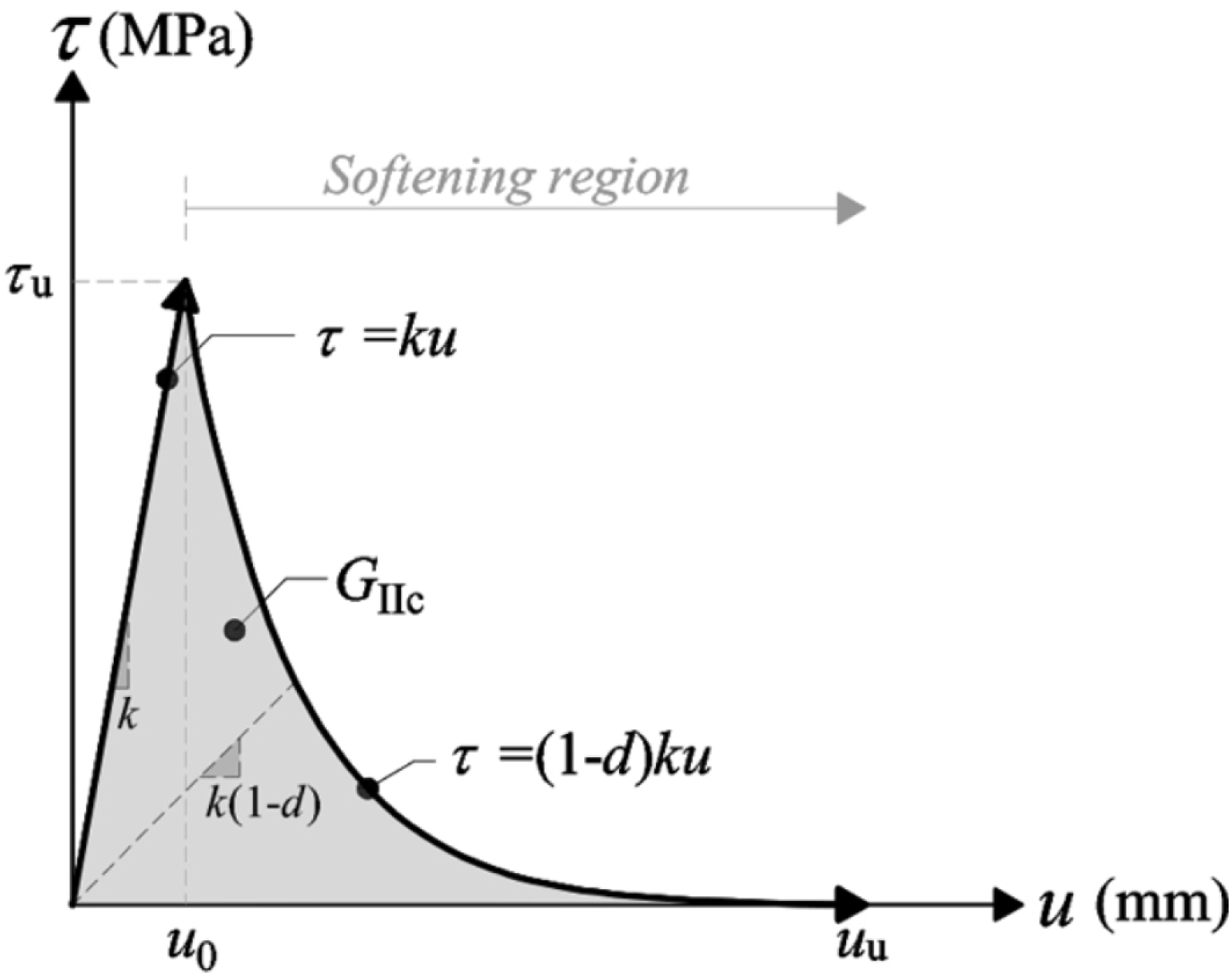
Additionally, the simplified FEM model that was already used for the verification of the analytical model was modified to simulate the torque–twist response of the PFSJ that can be compared with the experimental results. Such model can be useful to engineers modeling the joint within a bigger assembly with the need for a less simplified behavior, but not necessarily to analyze the stresses inside the joint. The model has two variants. Both of them represent the contact between steel and FRP as smooth surfaces with overclosure in mutual contact to induce pressure between these layers. In one variant, the contact is modeled using slip rate dependent friction. The other variant uses cohesive contact with the traction-separation law and exponential softening⁴¹ coupled with friction behavior. The traction-separation behavior is shown in Figure 25. Using de facto a superposition of these behaviors achieves damage initiation at defined shear stress, exponential softening, and then maintaining the constant torque response after failure.

Figure 25.

Shear traction–separation law with exponential damage evolution.⁴².

The data from the strain gauges during press-fitting showed the average value of strain to be 8.7 ⋅ 10⁻⁴. With consideration of longitudinal Young’s modulus 391 GPa of CN80 fiber composite provided by the manufacturer, this strain corresponds to a value of the tangential stress σ_t around 340 MPa. This then corresponds to interference δ = 0.08 mm in the analytical model, which equals to 20% of tooth tip height considering perfect geometry.

The data from the static test (Figure 26) showed that after a failure when reaching the maximum torque, there is a phase when the torque decreases and then remains constant, while the sample is still twisted, and the twist angle is increasing. Such torque can be called a residual. The maximal moment can then be used to determine the last unknown parameter of the analytical model, which is the friction coefficient f.

Figure 26.

Comparison: experiment - FEM simulation.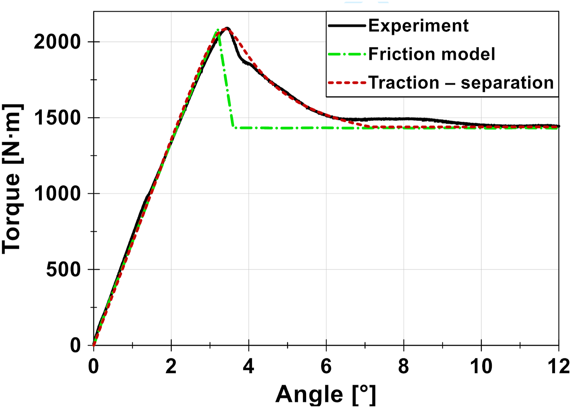

The value of the maximal torque is approx. 2100 N⋅m which corresponds with parameter f = 0.37. Along with the value of δ being equal to 20% of tooth height, this experiment determined the missing variables of the analytical model.

Based on the experiment, the parameters for the traction-separation behavior were set. Namely, stiffness k = 1100 and max. shear stress τ_u = 9.2 MPa, then for damage evolution total/plastic displacment 1.1 mm and the exponential parameter 2.3.

The FEM model presented in this section has a very good correlation with the experimental data for both variants (see Figure 26). The traction-separation model, however, represents the softening of the material better, while the torque in the friction model drops instantly.

Conclusion

An unconventional method to connect metal shafts with composite tubes was implemented along with analytical and FEM models. The analytical model is based on thick walled cylinder theory coupled with classical lamination theory, and the results of contact pressures and damage correlate well with the equivalent FEM model. Such model will be used as a quick tool for designers to yield instant results, thus shortening the development time.

Additionally, two studies on the geometry of the PFSJ were conducted. The first is on the length of the reinforcing layer relative to the end of the the steel shaft. The results showed that reinforcing layer reaching beyond the steel-FRP contact causes undesired peaks in contact pressure and damage to the main layer. This peak can be flattened by designing the reinforcing layer to the end aligned with the shaft end, or 1 mm before. The trade-off is a slightly increased, yet manageable damage of the reinforcing layer, and decreased contact pressure p₀₁.

The second study delved into the geometry of the shaft spline. While the model had limitations, as it did not use orthotropic material with plasticity nor simulated cutting the grooves and damage caused by that (this effect was represented by initial overclosure between layers 2 and 3), it showed useful insight by comparing individual variants. The variant with the highest load capacity was with a tooth angle of 60° and tooth height of 0.8 mm, but it remains unclear if such intrusion does or does not induce too high damage. This simulation, however, proved itself to be extremely time inefficient in terms of computational time as well as preparation of the model, and emphasized the need for the simplified models such as the analytical one.

Lastly, the static torsion test was conducted on PFSJ with central diameter D 50 mm with tooth angle 80° and a tooth height h_t of 0.4 mm. The experiment made it possible to determine the parameters of the analytical model for the current geometry such as δ and f. The joint itself withstood maximum torque of 2100 Nm which corresponds to an average value of shear stress of 21.4 MPa. This value of shear strength underperforms adhesive joints that can commonly achieve strength around 30-40 MPa⁴³ but can degrade under higher temperatures as Wang et al. showed.⁴⁴ while PFSJ is expected to be more thermally stable. Higher temperatures can, of course, inflict more damage due to the negative thermal expansion coefficient that causes the tube to shrink with increasing temperature and increases pressure in the joint. Another aspect is fatigue life, which remains unknown, while it might play a significant role as splined joints are prone to fretting which does not occur in adhesive joints. Also, an axial motion can occur due fatigue caused by cyclical axial forces acting on the joint shaft. However, this was merely an initial design with the potential to achieve higher strength with better geometry according to the teeth geometry study. Such improvement can be realized using sharper teeth, or reducing pitch of the teeth which results in more teeth on the shaft circumference that can withstand higher load. The pitch can be further reduced by leaving out the centering diameter D next to each tooth and keeping it only at certain sections of the circumference.

Along with the experiment, another FEM model was made to capture the torque response to the twist angle. One approach using a friction model, and the second using traction - separation law combined with friction. The latter had a very good correlation with only 80 N⋅m maximum absolute error (4.5%) occurring during the damage evolution phase, but all of that was at the cost of poor time efficiency. Compared to the friction model, the computational time was roughly 8 times higher. Therefore, if there is no need to model the damage evolution, the friction model is a sufficient tool.

Although this work has been focused on automotive application, it can be extended and maybe find even better use in other fields such as aerospace, defense industry or machine tools. There are certainly applications in these fields where shafts, spindles, and rotors of all kinds need the connection of steel and composite material to transfer torque. On top of that, these are the fields where, unlike in automotive, costs may not be the topmost priority (can be outweighed, for example, by lightweighting), and where slightly more expensive materials and manufacturing complex shaped parts such as the splined shaft can be employed. The findings in this work can benefit researchers and engineers in these fields as well.

Footnotes

ORCID iDs

Lukas Kazda

Ctirad Novotny

Funding

The authors disclosed receipt of the following financial support for the research, authorship, and/or publication of this article: This research has been realized using the support of Technological Agency, Czech Republic, program National Competence Centres, project # TN02000054 Božek Vehicle Engineering National Center of Competence (BOVENAC).

Declaration of conflicting interests

The authors declared no potential conflicts of interest with respect to the research, authorship, and/or publication of this article.

Data Availability Statement

The data from the experiment and FEM models will be available from the corresponding author on request.

References

Agarwal

Sahoo

Mohanty

, et al. Progress of novel techniques for lightweight automobile applications through innovative eco-friendly composite materials: a review. J Thermoplast Compos Mater 2020; 33(7): 978–1013. DOI: 10.1177/0892705718815530.

Taub

Luo

. Advanced lightweight materials and manufacturing processes for automotive applications. MRS Bull 2015; 40(12): 1045–1054. DOI: 10.1557/mrs.2015.268.

Bmw i3 makes its world premiere. Reinforc Plast 2013; 57(5): 7. DOI: 10.1016/S0034-3617(13)70136-X.

Bubna

Wiseman

. Impact of light-weight design on manufacturing cost - a review of bmw i3 and toyota corolla body components. In SAE 2016 World Congress and Exhibition. SAE International, 2016. DOI: 10.4271/2016-01-1339.

Patel

. Design & analysis of composite drive shaft for automobile. SSRN Electron J 2020; 10: 13–20.

Lee

Sung Kim

Woon Kim

, et al. Design and manufacture of an automotive hybrid aluminum/composite drive shaft. Compos Struct 2004; 63(1): 87–99. DOI: 10.1016/S0263-8223(03)00136-3.

Abu Talib

AliBadie

AMA

Azida Che LahGolestaneh

NAF

, et al. Developing a hybrid, carbon/glass fiber-reinforced, epoxy composite automotive drive shaft. Mater Des 2010; 31(1): 514–521. DOI: 10.1016/j.matdes.2009.06.015.

Badie

Mahdi

Hamouda

AMS

. An investigation into hybrid carbon/glass fiber reinforced epoxy composite automotive drive shaft. Mater Des 2011; 32(3): 1485–1500. DOI: 10.1016/j.matdes.2010.08.042.

Khalid

Mutasher

Sahari

, et al. Bending fatigue behavior of hybrid aluminum/composite drive shafts. Mater Des 2007; 28(1): 329–334. DOI: 10.1016/j.matdes.2005.05.021.

10.

Gur

Wagner

. Damping properties and nvh modal analysis results of carbon fiber composite vehicle components. SAE Int J Mater Manf 2017; 10(2): 198–205. DOI: 10.4271/2017-01-0500.

11.

Qatu

Iqbal

. Transverse vibration of a two-segment cross-ply composite shafts with a lumped mass. Compos Struct 2010; 92(5): 1126–1131. DOI: 10.1016/j.compstruct.2009.10.007.

12.

Kazda

Rika

Achtenová

, et al.

Effective use of composite materials in gearbox design for an electric vehicle. 9

2021. DOI: 10.46720/f2020-mml-058.

13.

Palermo

Britte

Janssens

, et al. The measurement of gear transmission error as an nvh indicator: theoretical discussion and industrial application via low-cost digital encoders to an all-electric vehicle gearbox. Mech Syst Signal Process 2018; 110: 368–389. DOI: 10.1016/j.ymssp.2018.03.005.

14.

Petr Bernardin . Spojování kompozitních materil s kovem. https://hdl.handle.net/11025/24958 (2016).

15.

Mcintyre

Davis

. WO1993022127A1 - Bonding of thermoplastic and thermoset composite structures to metallic structures - google patents, 4 1992. https://patents.google.com/patent/WO1993022127A1/de

16.

, et al. Influence of elevated temperatures on the bond performance of cfrp-steel lap joints bonded by nanosilica-modified adhesive with mixed curing agents. Constr Build Mater 2024; 426: 136131. DOI: 10.1016/j.conbuildmat.2024.136131.

17.

Guo

Liu

Y-L

Gao

W-Y

, et al. Bond behavior of cfrp-to-steel bonded joints at different service temperatures: experimental study and fe modeling. Constr Build Mater 2023; 362: 129836. DOI: 10.1016/j.conbuildmat.2022.129836.

18.

Zhang

Feng

, et al. Performance evolution of epoxy adhesive and cfrp-steel epoxy-bonded joints subjected to hygrothermal exposure. Constr Build Mater 2024; 429: 136445. DOI: 10.1016/j.conbuildmat.2024.136445.

19.

Qin

Zheng

, et al. Influence of single or multi-factor coupling of temperature, humidity and load on the aging failure of adhesively bonded cfrp / aluminum alloy composite joints for automobile applications. Int J Adhesion Adhes 2023; 123: 103345. DOI: 10.1016/j.ijadhadh.2023.103345.

20.

Heshmati

Haghani

Al-Emrani

. Durability of cfrp/steel joints under cyclic wet-dry and freeze-thaw conditions. Compos B Eng 2017; 126: 211–226. DOI: 10.1016/j.compositesb.2017.06.011.

21.

Lee

. Torque transmission capability of composite–metal interference fit joints. Compos Struct 2007; 78(4): 584–595. DOI: 10.1016/j.compstruct.2005.11.021.

22.

Cheng

Zhang

, et al. Modeling of damage behavior of carbon fiber reinforced plastic composites interference bolting with sleeve. Mater Des 2020; 194: 108904. DOI: 10.1016/j.matdes.2020.108904.

23.

Ružička

Uher

Blahouš

, et al. Computational design and static and fatigue tests of high-performance integrated joints. Mech Compos Mater 8 2010; 46(3): 317–322. DOI: 10.1007/s11029-010-9148-8.

24.

Gerhard

Friedrich

. Mechanical fastening of carbon composite tubes, numerical calculation of axial loading capacity and experimental verification. Compos B Eng 2014; 67: 391–399. DOI: 10.1016/j.compositesb.2014.07.024.

25.

Katz

Klimach

Haupt

, et al. Structural optimization and experimental investigation of cfrp lock nuts. Compos Appl Sci Manuf 2019; 117: 156–168. DOI: 10.1016/j.compositesa.2018.11.004.

26.

Meram

Can

. Experimental investigation of screwed joints capabilities for the cfrp composite laminates. Compos B Eng, 176:107142, 2019. DOI: 10.1016/j.compositesb.2019.107142.

27.

Jarrett

Jeffs

Korkees

, et al. The opportunities and challenges of hybrid composite driveshafts and their couplings in the aerospace industry: a review. Compos Struct 2023; 320: 117203. DOI: 10.1016/j.compstruct.2023.117203.

28.

James Dewhirst

Davidson

. US7731593B2 - composite transmission shaft joint - google patents, 3 2005.

29.

James Dewhirst

. US7874925B2 - transmission shaft joint design - google patents, 1. https://patents.google.com/patent/US7874925B2/en (2006).

30.

Michael Dewhirst and Lentus Composites Limited . WO2020109766A1 - attachment of an end fitting to a composite material tube - google patents, 11 2018. https://patents.google.com/patent/WO2020109766A1/en?oq=WO2020109766A1

31.

Lewis

Dewhirst

Composites Ltd

. US20200378433A1 - drive shaft - google Patents, 3. https://patents.google.com/patent/US20200378433A1/en?oq=16496781 (2017).

32.

Dale Faulkner and Will Pollitt . EP3473874A1 - splined end fittings - google patents, 10. https://patents.google.com/patent/EP3473874A1/en (2017).

33.

Nakamura

Kimoto

Fujikura Rubber Ltd . US8876614B2 - FRP drive shaft - google patents, 8. https://patents.google.com/patent/US8876614B2/en?inventor=Takato+Nakamura (2009).

34.

Nakamura

Okochi

Kimoto

, et al. Honda motor Co Ltd, and Fujikura Rubber Ltd. US10138925B2 - FRP drive shaft - Google Patents, 5, 2014. https://patents.google.com/patent/US10138925B2/en?inventor=Takato+Nakamura

35.

George

. Housner and Thad Vreeland. The analysis of stress and deformation. 1. https://ci.nii.ac.jp/ncid/BA10071031 (1966).

36.

Vincenzo Vullo . Circular cylinders and pressure vessels. 1 2014. DOI: 10.1007/978-3-319-00690-1.

37.

Croccolo

De Agostinis

. Analytical solution of stress and strain distributions in press fitted orthotropic cylinders. Int J Mech Sci 2013; 71: 21–29. DOI: 10.1016/j.ijmecsci.2013.03.002.

38.

French

Widden

. Stresses in thick-walled cylinders: a simple and insightful treatment. Int J Mech Eng Educ 1995; 23(3): 237–244. DOI: 10.1177/030641909502300308.

39.

Hashin

. Failure criteria for unidirectional fiber composites. J Appl Mech 1980; 47(2): 329–334. DOI: 10.1115/1.3153664.

40.

Nettles

. Basic mechanics of laminated composite plates , 10. https://ntrs.nasa.gov/api/citations/19950009349/downloads/19950009349.pdf (1994).

41.

ABAQUS/Standard User’s manual, version 2019. Dassault Systèmes Simulia Corp, United States, 2019.

42.

Luis Gómez-Royuela

Majano-Majano

Lara-Bocanegra

, et al. Shear traction-separation laws of European beech under mode II loading by 3D digital image correlation. Wood Sci Technol, 56(6):1631–1655, 11 2022. DOI: 10.1007/s00226-022-01429-3.

43.

Banea

da Silva

LFM

. Adhesively bonded joints in composite materials: an overview. Proc Inst Mech Eng, Part L 2009; 223(1): 1–18. DOI: 10.1243/14644207JMDA219.

44.

Wang

Gao

Ding

, et al. Bond strength between carbon fiber–reinforced plastic tubes and aluminum joints for racing car suspension. Adv Mech Eng 2016; 8(10): 1687814016674627. DOI: 10.1177/1687814016674627.