Sage Journals: Discover world-class research

Abstract

Composite materials, such as Carbon Fiber Reinforced Plastics (CFRP), are widely used across industries due to their exceptional mechanical properties and lightweight nature. With increasing interest in hydrogen storage applications, a comprehensive understanding of CFRP’s microstructure is crucial. However, there remains a critical gap in effectively linking microstructural characteristics to multiscale simulation models for improved tank design. This study presents a detailed analysis of CFRP microstructure using micro-section image analysis. Advanced artificial intelligence techniques, including transfer learning with VGG16 and XGBoost, are employed to detect fibers and matrix-rich regions. Notably, the model achieves an impressive Area Under the Receiver Operating Characteristic (AUC) of 0.89, providing strong quantitative validation. Furthermore, the experimentally determined fiber volume fraction of 0.59 closely aligns with the predicted value of 0.589, demonstrating the model’s accuracy. The investigation extends to analyzing fiber distribution using statistical features such as Voronoi polygons and kernel density estimation. Through dimensionality reduction via t-SNE and clustering, distinct patterns in CFRP’s microstructure are identified, offering deeper insights into its complexity. Finally, an explainable artificial intelligence (XAI) framework is implemented using a surrogate model to map the decision-making process to microstructure characteristics. The surrogate model achieves an F1-score of 0.90, reinforcing the reliability of the approach. This research provides valuable insights into the distinct categories in CFRP’s microstructure, particularly relevant for utilization in multiscale numerical methods.

Keywords

Microstructure convolutional neural network eXtreme gradient boosting t-SNE,pattern recognition Surrogate eXplainable artificial intelligence

Introduction

The imperative transition toward a sustainable and decarbonized environment has fueled a growing global demand for hydrogen as a clean fuel source. The realization of hydrogen-powered propulsion systems necessitates advancements in storage technologies, placing a particular spotlight on the development of efficient and reliable hydrogen storage systems in critical fields such as aerospace and automotive.The storage of hydrogen is challenging as it requires holding it at significantly high pressure (350 − 750 bar).¹ Due to its superior weight-to-strength ratio and better mechanical, thermal, and chemical characteristics, CFRP has proved to be a suitable candidate for this application.

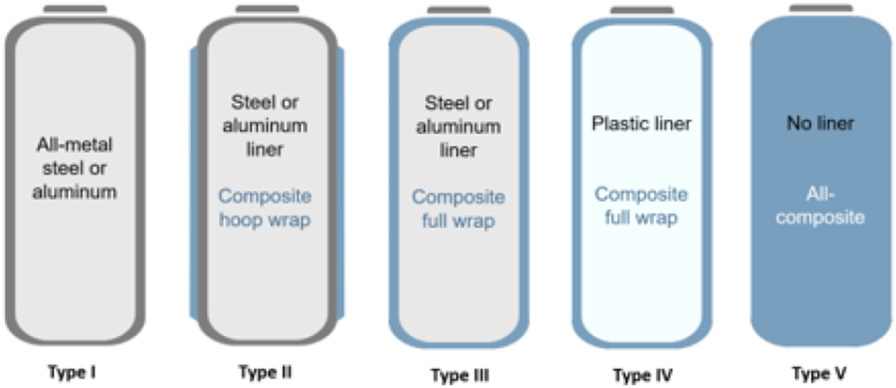
Hydrogen storage systems can be categorized as shown in Figure 1. Composite over-wrapped pressure vessels, such as Types 2 to 4, utilize CFRP to sustain structural loads. The state-of-the-art storage tank used in commercial applications is a type 4 tank, despite of advanced type 5 design. These tanks consist of an inner polymer liner to restrict gas permeation and a CFRP over-wrap to bear mechanical loads.³ Manufacturing techniques such as filament winding⁴ and automated fiber placement (AFP)⁵ are commonly employed for their fabrication.

Figure 1.

A schematic describing types of storage tanks for hydrogen.²

Advancements in CFRP-based structures have demonstrated improvements in storage efficiency and weight reduction.⁶ However, gaps in understanding failure mechanisms at different length scales pose challenges in their overall application. Evidently, micro-cracks in the CFRP can combine to crack networks and lead to leakage and influence structural integrity at higher levels.^7,8 Therefore, a high-fidelity multi-scale approach is required, where microstructural insights inform meso- and macro-level models for accurate material behavior predictions, particularly in areas such as burst pressure and leakage analysis.

Several studies^9,10 have highlighted the significant influence of fiber arrangements on fiber-matrix bonding, which ultimately dictates crack initiation and propagation. This phenomenon is primarily attributed to the property mismatch at the fiber/matrix interface, leading to a stress concentration around the fibers and often resulting in inter-facial failure¹¹ and advocating the importance of the fiber distribution. Additionally, the intricate manufacturing process and functional environment, characterized by varying temperature steps, can give rise to numerous matrix cracks, particularly in materials intended for applications such as liquid hydrogen storage, which undergo cryogenic thermal loads. These thermal stresses induce differential expansion between the matrix and fibers, given the substantial difference in their coefficients of expansion of more than two order.¹²

The application of thermal loads leads to matrix embrittlement, consequently affecting the region with higher resin packing density and resulting in higher unidirectional (UD) strengths.¹³ However, this also correlates with an increased occurrence of micro-cracks due to purely thermal loads.¹⁴ The continuous occurrence of such inter-facial failure and thermally induced matrix cracking may lead towards the contribution of a through-thickness crack.¹⁵ Further thermal and mechanical loading may help join multiple micro-cracks to form a network.^16–19

In conclusion, the distribution of fibers within carbon composites significantly impacts the formation of micro-cracks especially the under cryogenic loading.²⁰ Non-uniform distribution can lead to stress concentrations, and weak points, which may lead to higher crack density and eventually a leakage through thickness crack.²¹

Traditionally, micro-level FEM analysis employed simplified periodic fiber²² arrangements within single fiber unit cell models. However, these models fall short of representing the skewed distribution of fibers observed in real-life scenarios as in Figure 2. Several research used different approaches by utilizing modified versions of random fiber generation with specific fiber volume fraction.^23–26 However such studies are not free from problems. Random fiber generation can lead to increased computational complexity due to the need to generate and analyze a large number of different configurations.²⁷ This could potentially slow down the simulation process, especially for complex geometries or materials. While random fiber generation can provide useful insights into the behavior of CFRP composites, it may not accurately predict the real-world performance of the material, as the random nature of the fiber distribution may not fully represent the actual fiber distribution in a real composite material.²⁸ More advancements can be seen in the works of²⁹ and,³⁰ where the authors have devised several methods to analyze microstructure by detecting fibers and using this information for generating a realistic representative volume element (RVE). However, these methods encounter challenges in characterizing a single RVE that can faithfully represent the diverse architecture of fiber distribution.

Figure 2.

Different microstructure demonstrating varied fiber distribution.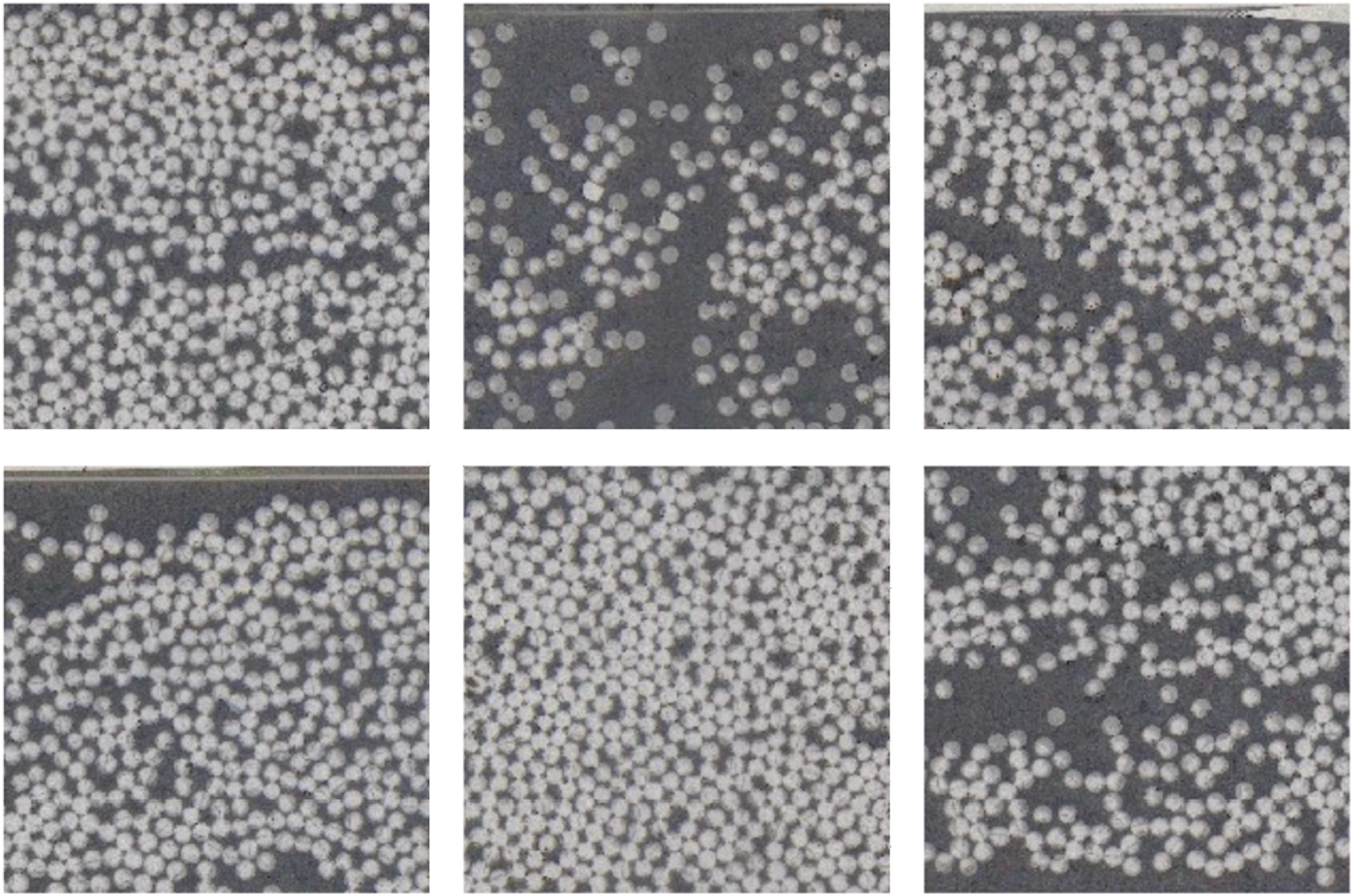

Despite these advancements, there remains a lack of frameworks that both capture realistic microstructural diversity and systematically link it to higher-scale material behavior predictions, particularly for leakage in hydrogen tanks. This study addresses this gap by developing an XAI-based methodology that bridges microstructural characterization and multiscale modeling needs.

Machine learning has emerged as a powerful tool to address these challenges by extracting meaningful insights from complex datasets and improving predictive accuracy. In 31, authors developed a Gaussian Process Regression (GPR) model utilizing drilling parameters such as cutting speed, drill size, and feed rate. Their study demonstrated that the GPR model provided stable and accurate predictions of the delamination factor, highlighting both the complexity of analyzing CFRP materials and the potential of machine learning in extracting meaningful insights from complex datasets. Similarly, in 32, author developed Multivariate Linear Regression (MLR) and GPR models based on mixture proportions, including the EVA:starch ratio, glycerin content, and NaHCO₃ content. Their study demonstrated that these models produced predictions closely matching experimental values. The authors suggest that these approaches can aid in designing mixture proportions and identifying statistical correlations between components and mechanical properties in starch-based foams. This underscores the value of machine learning in uncovering numerical relationships between input parameters and performance metrics, as well as its broader applicability in analyzing complex material systems.

Building on these advancements, this work introduces a novel XAI framework capable of accurately characterizing a finite set of distinct microstructure types. By combining advanced machine learning techniques with interpretable decision-making, the framework provides deeper insights into the fundamental patterns governing fiber distribution. This enhanced understanding supports material design, optimization, and performance prediction. Additionally, the explainability of the surrogate models strengthens user confidence, establishing the framework as a reliable tool for informed decision-making.

The remainder of the presented paper is organized as follows. Section 2 describes the manufacturing of specimens and micro-section extraction to supply data for fiber distribution analysis. In Section 3, a brief overview of the existing methods to detect fibers and their shortcomings are discussed. Further, a detailed description of the employed methods to detect fibers, statistical properties to describe the microstructure and later its characterization is presented. Section 4 offers a detailed insight into the results and performance evaluation of the machine learning models. Section 5 deals with the eXplainable Artificial Intelligence framework using surrogate models and their result interpretation and performance evaluation. Lastly, Section 6 presents a summary of the presented work with an outlook.

Experiment and data

Manufacturing and testing

The specimens were manufactured using unidirectional CFRP prepreg provided by Hexcel (HexPly 8552/35%/134gsm/IM7), with a nominal cured ply thickness of 0.125 mm. Two types of plates were produced, each with a nominal thickness of 2 mm but differing in stacking sequence: namely, [0,90]_8s and [0₂, 90₂]4s.

The layup was performed manually, followed by vacuum bagging and curing in accordance with the manufacturer’s recommended cycle. After curing, small 15 × 15 mm samples were extracted by milling (as illustrated in Figure 3) and subsequently embedded in resin for microscopy.

Figure 3.

A Schematic describing the specimen opted for microscopy.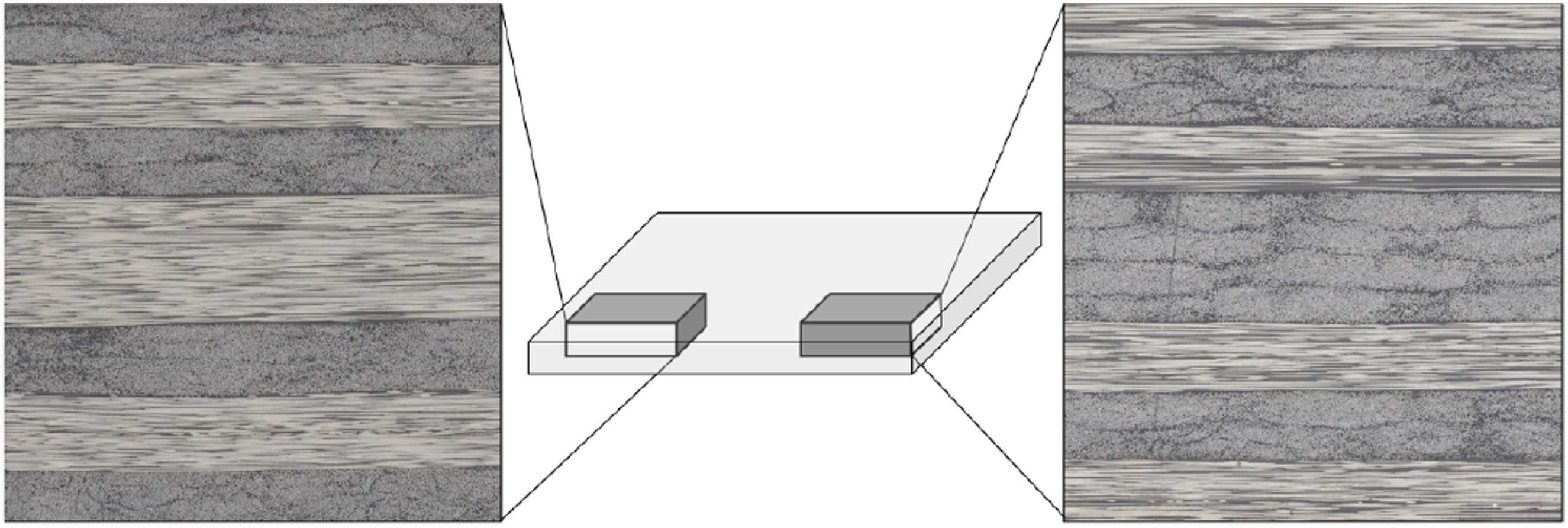

Digital microscopy

To capture the fiber distribution within the composite laminate, microscopy experiments were conducted on a specimen at a 50x zoom level with a resolution of 0.67 micron. This allowed for detailed imaging of the laminate’s cross-section, highlighting the arrangement and spatial distribution of the fibers. The obtained images were stored for further analysis, enabling the characterization of the fiber distribution and subsequent evaluation of its impact on composite performance.

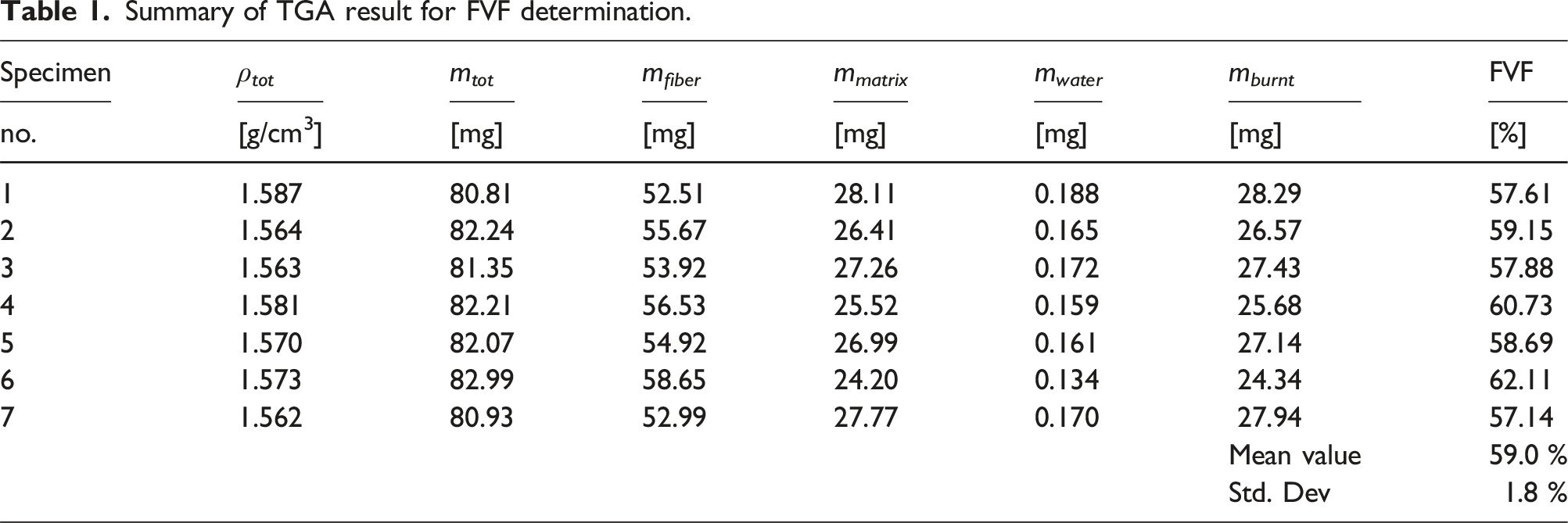
Experimental determination of fiber volume fraction

Determination of the fiber volume fraction (FVF) is done by thermogravimetric analysis (TGA) by DIN 16459:2021-06. The specimens are 7 × 7 mm in size and 2 mm in thickness. The decomposition of the matrix to determine mass loss is carried out under synthetic air with reduced heating rates to prevent uncontrolled combustion with a sharp increase in heat flow in the measuring cell. The process consists of four steps: heating of the specimen to 140°C at a heating rate of 20°C/min; isothermal holding step at 140°C, heating to 450°C at 10°C/min and an isothermal holding phase of up to 230 min. The fiber volume fraction is calculated using the mass m and density ρ of the fiber and specimen, respectively:

F V F = \frac{m_{fiber}}{m_{specimen}} \cdot \frac{ρ_{specimen}}{ρ_{fiber}} [\cdot 100 %]

(1)

Table 1 shows the result of the FVF determination through TGA, where the fiber density ρ_fiber is assumed to be 1.79 g/cm³.

Table 1.

Summary of TGA result for FVF determination.

Specimen	ρ _tot	m _tot	m _fiber	m _matrix	m _water	m _burnt	FVF
no.	[g/cm³]	[mg]	[mg]	[mg]	[mg]	[mg]	[%]
1	1.587	80.81	52.51	28.11	0.188	28.29	57.61
2	1.564	82.24	55.67	26.41	0.165	26.57	59.15
3	1.563	81.35	53.92	27.26	0.172	27.43	57.88
4	1.581	82.21	56.53	25.52	0.159	25.68	60.73
5	1.570	82.07	54.92	26.99	0.161	27.14	58.69
6	1.573	82.99	58.65	24.20	0.134	24.34	62.11
7	1.562	80.93	52.99	27.77	0.170	27.94	57.14
						Mean value	59.0 %
						Std. Dev	1.8 %

Methods

In this section, a brief review of existing image analysis methods is done to explore the possibilities to study fiber distribution. Later a framework is introduced to segregate the fibers from the matrix bulk material and the coordinates are studied to draw further conclusions.

Conventional methods for fiber detection

Hand labeling

A systematic analysis is used to derive the spatial fiber distribution from the acquired images. The complete microscopy image was cropped into smaller snapshots (as in Figure 4(a)), each measuring 125 x 125 micron square. These smaller snapshots allow a focused examination of localized fiber arrangements within the laminate. An open-source Python plug-in named Label-studio³³ is employed to detect the fibers within these snapshots. This plug-in facilitated the manual identification and labeling of the fibers present in each snapshot. For illustration, in Figure 4 an original snapshot (a) of size 125 x 125 micron with its hand-labeled fiber annotation (b) is depicted.

Figure 4.

Micro-section images, (a) Original snapshot from micro-section, (b) Hand-labeled image using Label-Studio, (c) Pixel thresholding result, and (d) Fiber detection using Hough Transformation.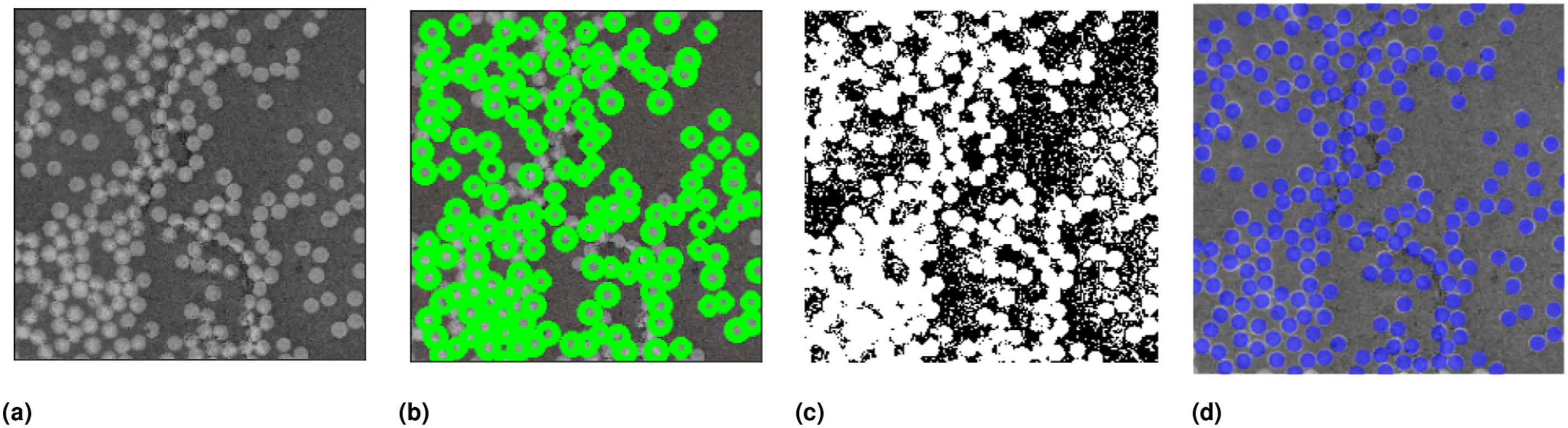

The annotations are later exported as images and used for training and testing machine learning models. However, this manual detection process proved tedious and time-consuming, requiring significant effort to accurately identify and label each fiber.

Pixel thresholding

Pixel thresholding is a basic image processing technique used to segment an image into distinct regions based on pixel intensity values. It involves setting a threshold value and classifying each pixel as either foreground or background based on its intensity compared to the threshold. The results of pixel thresholding are depicted in Figure 4(c). Due to the intricate specimen preparation process and image artifacts, it is difficult to rely only on the pixel intensity as a metric to segment fibers. Further, a unique threshold for all the snapshots for a wide range of specimens can be a non-trivial task, therefore other image analysis techniques are investigated.

Hough transformation

The Hough circles transformation³⁴ is a popular image processing technique to detect circles in digital images. It is an extension of the Hough line transformation and is particularly useful for identifying circular shapes, such as objects, patterns, or structures.

The Hough circles transformation involves converting an image from the Cartesian coordinate system to the Hough parameter space. In this parameter space, each circle is characterized by three parameters: the x and y coordinates of its center and its radius. Consequently, every pixel in the image contributes to the generation of a circular equation in the Hough parameter space. However, the performance of the Hough circles transformation is strongly sensitive towards parameters such as the threshold for peak detection, which need to be appropriately set based on the specific application and image characteristics. It is also limited to detecting only perfect circles, which could be a setback as micro-section images are not exempt from noise. Moreover, the computational efficiency of Hough transformation gradually decreases with increasing amount of noise and image size (Figure 4(d)).

Problems and limitations

Due to the limitations and laborious nature of manual fiber detection, alternative image analysis techniques are explored to streamline the fiber distribution analysis process. Initially, methods such as Hough circles and pixel thresholding were implemented to automatically detect fibers. However, these techniques presented challenges, as they required the adjustment of multiple parameters and often produced faulty fiber detections, further extending the analysis time. For instance, pixel thresholding requires a unique threshold for a successful segmentation of the fibers from the bulk material. However, it is non-trivial to assign a threshold for every micro-section image. Further, the presence of noise makes it even more challenging as it increases the false detection.

A comprehensive framework may enable more effective analysis of fiber distribution within manufactured specimens. Together with a robust numerical model, a deeper understanding and improved prediction of micro-crack formation and propagation can be obtained. This type of analysis is particularly important for preserving the structural integrity of cryogenic tanks, where micro-cracks may pose serious risks.

Machine learning framework

The machine learning framework proposed in this study consists of multiple steps, as illustrated in Figure 5. First, raw microscopy images undergo preprocessing before being fed into a VGG16 deep convolutional neural network, which serves as a feature extractor. The high-quality features obtained from VGG16 are then used to train an XGBoost model to generate a binary map, where fiber pixels are labeled as 1 and the matrix as 0. Next, DBSCAN clustering is applied to the binary map to group fiber pixels based on their proximity and density, effectively distinguishing individual fibers. The coordinates of these fibers are then analyzed to study their spatial arrangement using statistical methods such as Voronoi polygons and kernel density estimation. These statistics enables us to quantify fiber distribution in-terms of their sparsity and density. These statistics are discussed in detail in section 3.3. The resulting high-dimensional spatial features are subsequently reduced to a more manageable 2D or 3D representation using t-SNE. Finally, K-means clustering is employed to identify distinct microstructure groups.

Figure 5.

Complete machine learning framework for microstructure clustering. Step-1: Optical microscopy to record fiber distribution; Step-2: Deep learning model for feature extraction; Step-3: XGB model for semantic segmentation from VGG16 features; Step-4: DBSCAN clustering to clusters fiber pixels into distinct fibers; Step-5: Extract spatial detected fibers using Voronoi polygona nd Kernel density estimation; Step-6: Dimensionality reduction and clustering in lower dimension for microstructure clustering.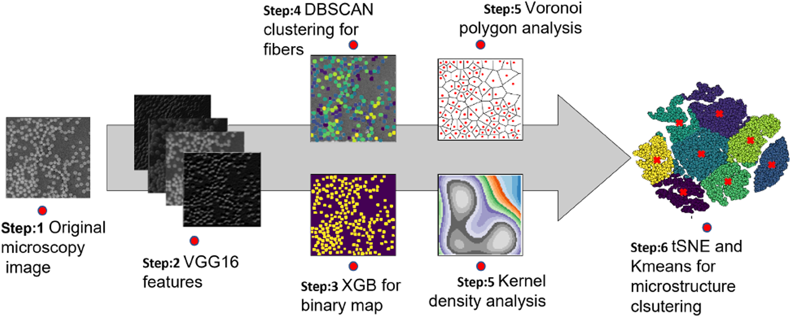

Deep convolutional neural networks for feature extraction

VGG16³⁵ is a deep convolutional neural network (CNN) architecture that has proven effective in various computer vision tasks, including image classification. It consists of 16 convolutional layers, hence the name VGG16, followed by fully connected layers. It is known for its simplicity and uniformity in architecture, with all convolutional layers having a 3 × 3 filter size and a stride of 1, and all max-pooling layers using a 2 × 2 window with a stride of 2. This uniformity allows for straightforward implementation and easy interpretation of the network.

The VGG16 architecture with an ImageNet³⁶ backbone has been pre-trained on a large-scale dataset. This pre-training process enables the network to learn general features from a diverse range of images, making it a powerful tool for transfer learning. The utilization of the pre-trained VGG16 network with an ImageNet backbone allows the extraction of relevant information from the cropped images of the composite laminate, leveraging the learned features. The original images (as in Figure 4(a)) were inputted into the VGG16 network, and the convolutional layers were utilized to capture hierarchical representations of the image features.

To focus on the discriminative features specific to our composite laminate images, we decided to chop the VGG16 network right after the feature extraction (as in Figure 6) from the convolutional layers. This allowed us to retain the high-level features extracted by the convolutional layers while discarding the fully connected layers responsible for classification. Bypassing the cropped laminate images through the modified VGG16 network, we obtained a set of feature vectors representing the extracted features. These feature vectors captured the essential information about the spatial arrangement and characteristics of the fibers within the laminate. Such features with label data from label-studio were used as training and testing data for a subsequent machine learning model, eXtreme Gradient Boosting (XGBoost).

Figure 6.

A schematic representing the presented machine learning framework for microstructure characterization.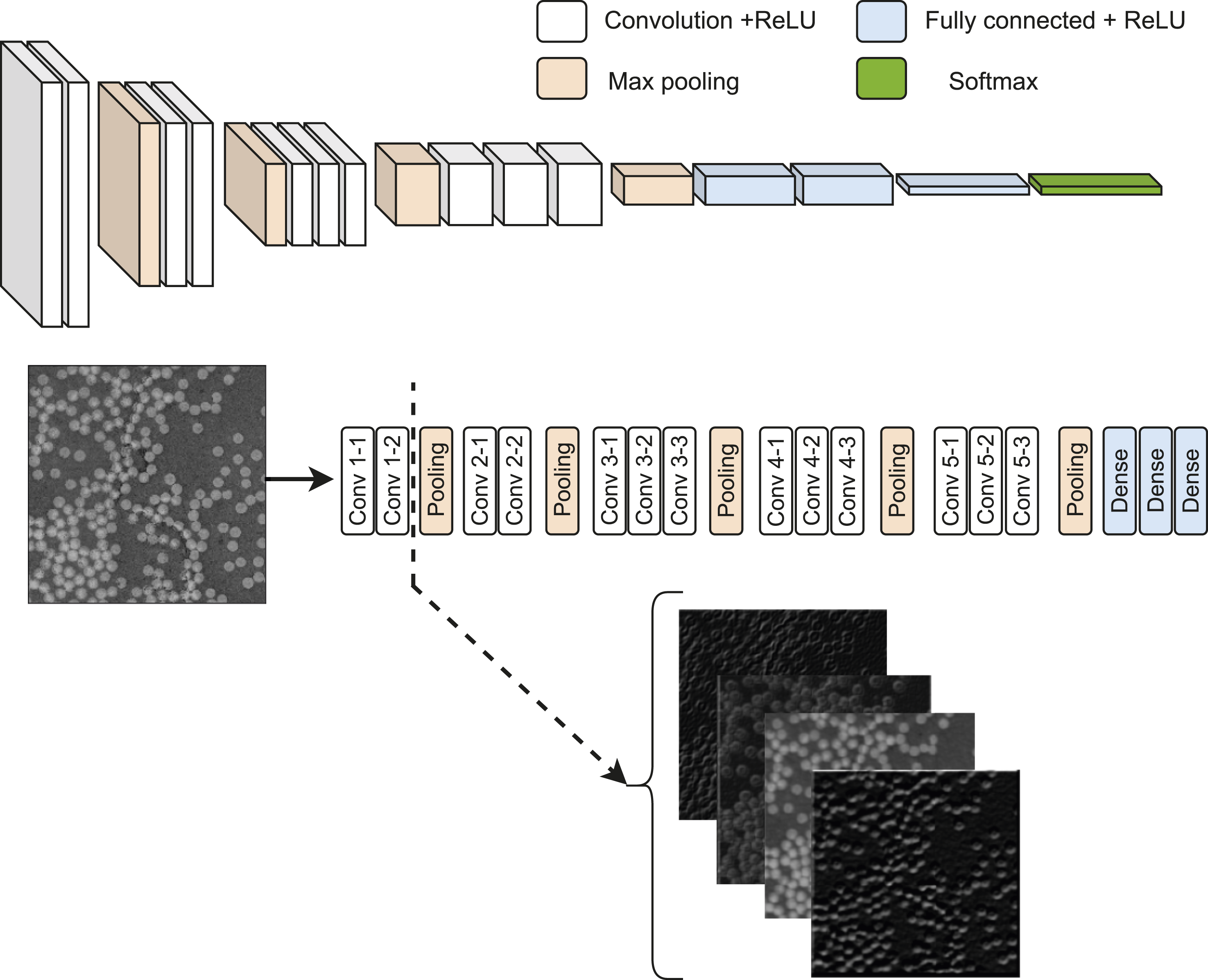

Fiber detection using eXtreme gradient boosting

XGBoost³⁷ is a powerful machine-learning algorithm that has gained significant popularity in both academic research and practical applications. It is known for its exceptional performance in various classification tasks. XGBoost is an ensemble method that combines the predictions of multiple individual models, called decision trees, to make accurate predictions.

As a classifier, XGBoost uses training data with known labels to build a collection of decision trees. Here the features from the VGG16 model combined with the manual labeling with label-Studio is used as such dataset. During training, the algorithm learns to iteratively improve the weak learners (decision trees) by minimizing a specific loss function (log loss). Each subsequent tree is built to correct the errors made by the previous trees, resulting in a strong and accurate ensemble model, see Figure 7.

Figure 7.

A schematic diagram of XGBoost comprised of ’k’ number of trees.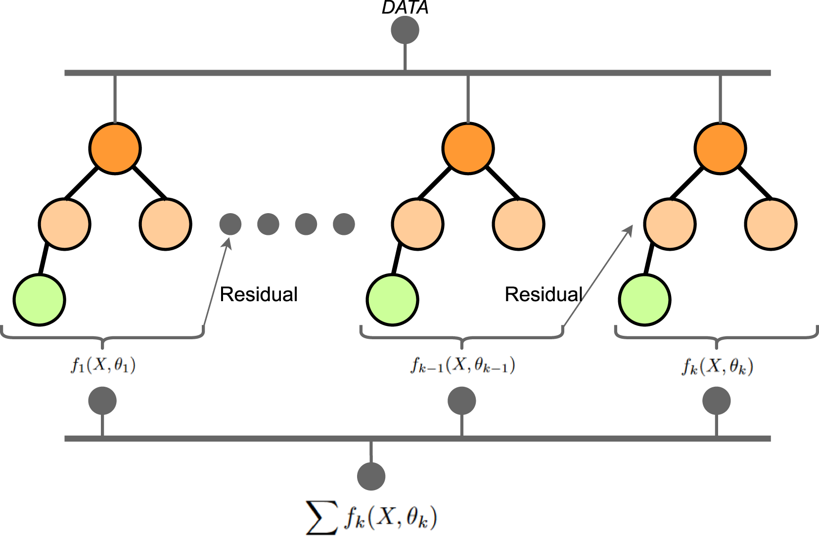

XGBoost incorporates several key techniques that contribute to its effectiveness as a classifier. It uses a gradient boosting framework, where each new tree is trained to minimize the gradient of the loss function concerning the ensemble predictions. Additionally, XGBoost implements regularization techniques to prevent overfitting, such as by controlling the complexity of individual trees or adding penalties to the objective function. For a given dataset containing ’m’ features and ’n’ data instances, the objective function for a tree ensemble model may be written as equation (2). Here L is a differentiable convex loss function, Ω is the penalty term for the model such that, Ω = γT + 1/2λ‖w‖². T is the number of leaves in the tree, w is the weight of the leaf, γ and λ are the regularization parameters helping the smooth learning of the weights and reducing over-fitting.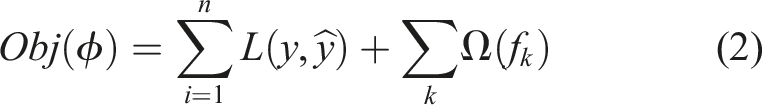

O b j (ϕ) = \sum_{i = 1}^{n} L (y, \hat{y}) + \sum_{k} Ω (f_{k})

(2)

For a gradient boosting scheme, the ensemble model is trained in an additive manner and greedily adds f_t, which can improve the learning significantly using equation (2).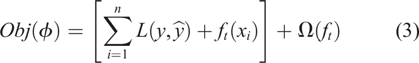

O b j (ϕ) = [\sum_{i = 1}^{n} L (y, \hat{y}) + f_{t} (x_{i})] + Ω (f_{t})

(3)

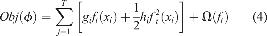
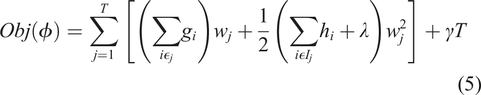
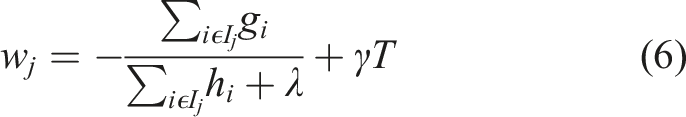
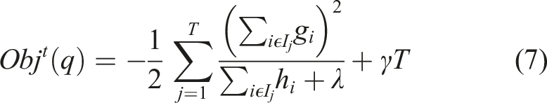
A second-order approximation is used to quickly optimize the objective function using Taylor-Series expansion and the equation (3) can be elaborated as follows. Here the $g_{i} = \partial L / \partial {\hat{y}}^{t - 1}$ , and $h_{i} = \partial L^{2} / {\partial {\hat{y}}^{t - 1}}^{2}$ are the first and second order derivatives of the loss.

O b j (ϕ) = \sum_{j = 1}^{T} [g_{i} f_{t} (x_{i}) + \frac{1}{2} h_{i} f_{t}^{2} (x_{i})] + Ω (f_{t})

(4)

Equation (4) can be re-written by expanding the penalty term Ω. Here w_j is the weight of the leaf or node and can be written for a fixed structure of a tree as q(x) (see equation (5)).

O b j (ϕ) = \sum_{j = 1}^{T} [(\sum_{i ϵ_{j}} g_{i}) w_{j} + \frac{1}{2} (\sum_{i ϵ I_{j}} h_{i} + λ) w_{j}^{2}] + γ T

(5)

w_{j} = - \frac{\sum_{i ϵ I_{j}} g_{i}}{\sum_{i ϵ I_{j}} h_{i} + λ} + γ T

(6)

The corresponding loss function for a given tree structure q(x) with the weight w_j (equation (6)) can be written as equation (7). This function can used as a purity score to dermine the quality of the split for a given tree structure q(x).

O b j^{t} (q) = - \frac{1}{2} \sum_{j = 1}^{T} \frac{{(\sum_{i ϵ I_{j}} g_{i})}^{2}}{\sum_{i ϵ I_{j}} h_{i} + λ} + γ T

(7)

However, it is impossible to compute a separate loss function for all the different tree structures, therefore a greedy algorithm is used to get the best objective function. This greedy algorithm starts with a single leaf and iteratively adds the branches to the structure of the tree. By setting I = I_L + I_R, where I is nodes/leaves for the left and right side for the corresponding sub-scripts, the generalized loss function can be for the split may be written as in equation (8).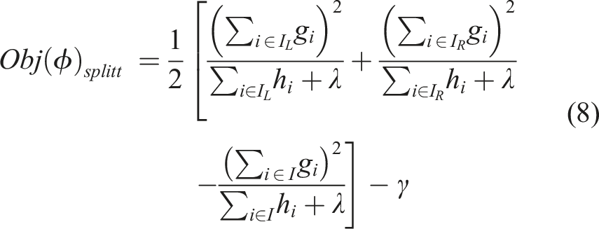

\begin{align} O b j {(ϕ)}_{splitt} & = \frac{1}{2} [\frac{{(\sum_{i \in I_{L}} g_{i})}^{2}}{\sum_{i \in I_{L}} h_{i} + λ} + \frac{{(\sum_{i \in I_{R}} g_{i})}^{2}}{\sum_{i \in I_{R}} h_{i} + λ} \\ - \frac{{(\sum_{i \in I} g_{i})}^{2}}{\sum_{i \in I} h_{i} + λ}] - γ \end{align}

(8)

Furthermore, XGBoost offers various hyper-parameters that can be tuned to optimize its performance for specific data sets. These include parameters related to the tree structure, regularization, learning rate, and more. The algorithm’s flexibility and scalability make it suitable for large-scale problems and high-dimensional data sets.

In the work, this XGBoost model was used to detect fiber pixels from a set of features from the VGG16 model. A stratified 80:20 train-test split was used to ensure balanced representation of different microstructure categories. To prevent overfitting, early stopping was applied with a patience of 10 rounds, using log-loss on a validation set (20% of the training data) as the evaluation metric.

The semantic segmentation result from the XGBoost algorithm yields a binary image see Figure 8, where 1 represents a pixel classified as fiber and the rest as 0 representing matrix. However, to completely understand the fiber distribution, one must get the fiber centers rather than the location of all the pixels classified as fibers. Therefore a well-known non-linear clustering algorithm was employed to cluster the pixels into distinct fibers.

Figure 8.

A schematic depicting feature maps from VGG16 model predicted into fibers using XGB model.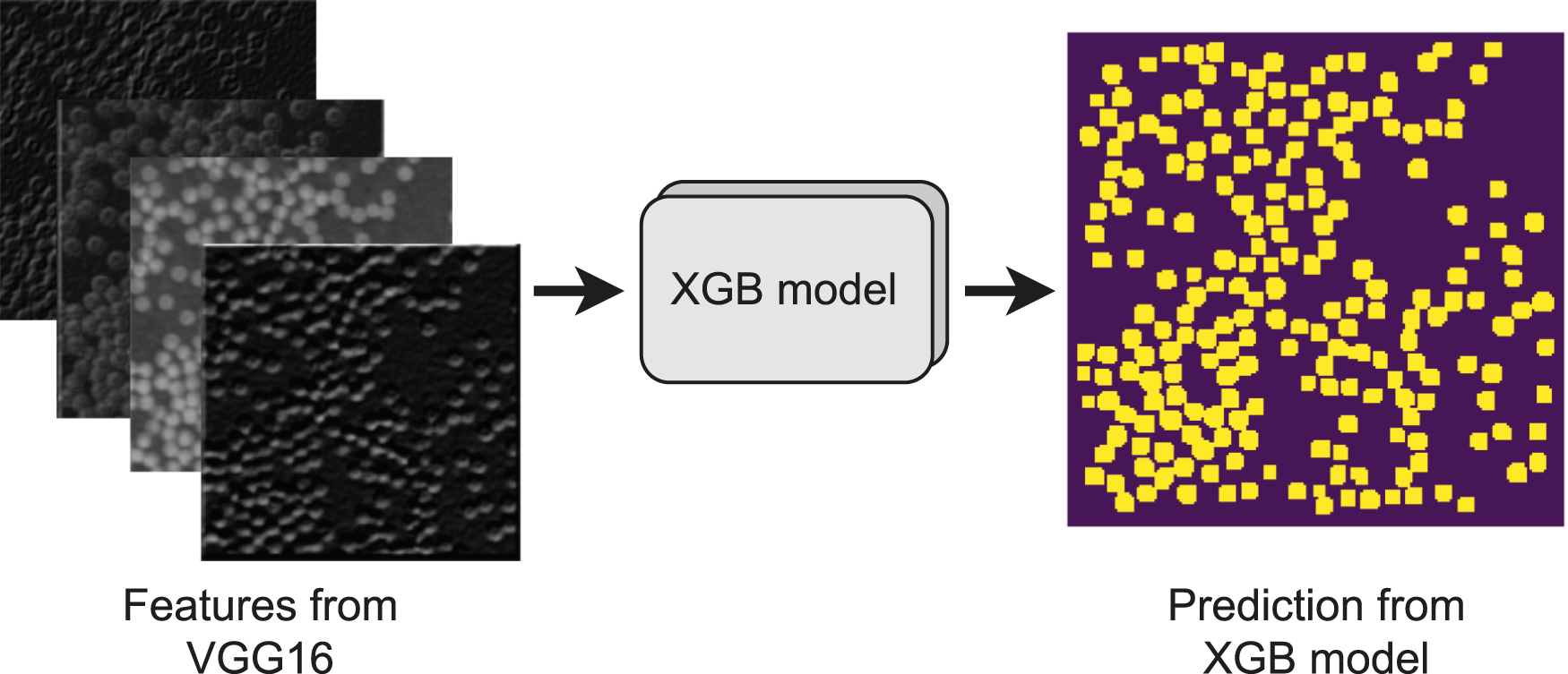

Clustering using DBSCAN

As mentioned earlier, a Density-Based Spatial Clustering of Applications with Noise (DBSCAN)³⁸ groups the neighboring pixels into a cluster. It is a density-based clustering algorithm commonly used for unsupervised learning tasks. Unlike traditional clustering algorithms that assume clusters have a specific shape, DBSCAN can discover clusters of arbitrary shape and effectively handle noisy data points. Here all the pixels classified as fibers from XGBoost are clustered into distinct fibers based on their density and spatial location.

As a clustering algorithm, DBSCAN does not require prior knowledge of the number of clusters (number of fibers in the presented case) in the data. Instead, it defines clusters as dense regions of data points separated by areas of lower density. The algorithm categorizes each data point (pixel in this case) into one of three categories: core points, border points, and noise points, using two user-defined parameters: the minimum number of points (minPts) and the epsilon radius (Eps). Core points are data points that have a sufficient number of neighboring points (minPts) within a specified distance (Eps). Border points are located within the epsilon radius of a core point but do not have enough neighbors to be considered core points themselves. Noise points, on the other hand, have neither enough neighbors nor fall within the epsilon radius of a core point (see Figure 9). DBSCAN operates by starting with an arbitrary data point and expanding clusters by connecting neighboring core points. It continues to grow a cluster until no more core points are found within the epsilon radius. This process repeats for other unvisited points until all data points have been assigned to a cluster or marked as noise.

Figure 9.

A schematic representing core points which has MinPts number of pixels in its Eps radius, border points, and noise/outliers.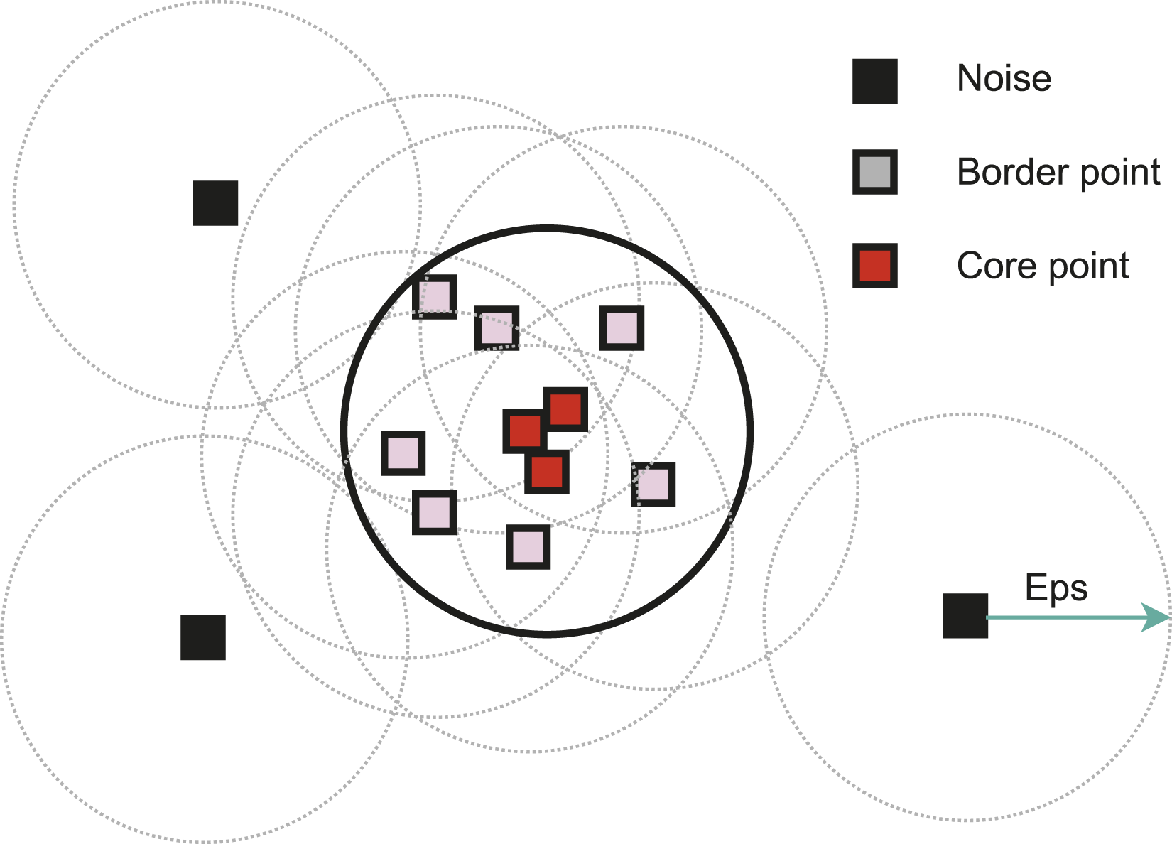

DBSCAN’s performance is dependent on two primary parameters: epsilon (Eps), which defines the radius around each data point, and the minimum number of points (MinPts) required to form a core point. These parameters influence the granularity and quality of the clusters discovered by the algorithm. Tuning these parameters appropriately is crucial for obtaining meaningful clustering results. This final step of the complete framework yields information such as the number of fibers detected (see Figure 10) in the given picture and the coordinates of each fiber center in the given domain. However, to get a complete understanding of the fiber distribution, further steps must be taken to analyze the fiber coordinates.

Figure 10.

Individual fibers detection from XGB binary map using DBSCAN.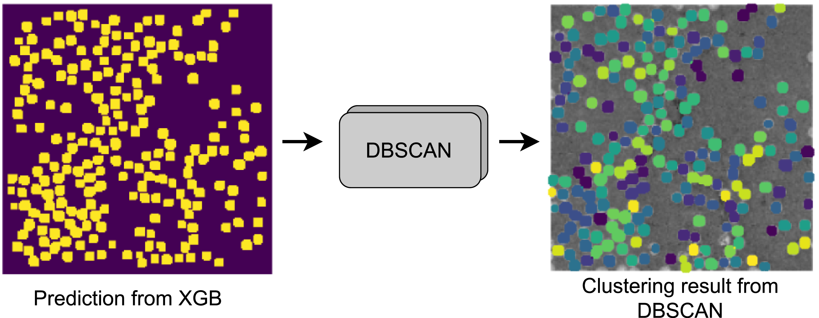

The clustering results from the DBSCAN algorithm, as depicted in Figure 10, reveal that several partially present fibers are not detected due to the algorithm categorizing them as noise. However, it is noteworthy that such fibers are indeed present in the neighboring microstructure and are accurately detected.

Quantification of homogeneity of fiber distribution

The non-linear clustering described in the previous section results in the clustering of the neighboring pixels into distinct fibers/clusters. Such clusters are later analyzed to obtain their centers as fiber centers. This information is crucial for understanding the fiber distribution and consequently tightness and looseness in the fiber packing.

Researchers have used several methods to describe a 2D spatial distribution which can help to quantify the homogeneity like Voronoi polygon analysis,³⁹ K-Ripley function,²⁸ and kernel density estimation.⁴⁰ Authors have used the mean Voronoi polygon area to quantify the gaps in the microstructure of carbon composites. Similarly,⁴¹ used the K-reply function to obtain the quantification for the fiber distribution.

In this work, similar methods like the Area fraction method, kernel density estimation function, and Voronoi polygon analysis were used to study the fiber distribution and quantify the microstructure based on the tightness and looseness of the fiber packing.

Area fraction method

The area fraction method is used to calculate the fiber volume fraction in a given domain or material. It is commonly employed in composite materials, where fibers are embedded in a matrix. It estimates this value by measuring the fraction of the total cross-sectional area covered by the fibers in our case pixels of fibers in a representative sample. This can be readily computed using the results from the DBSCAN algorithm using equation (9).

Area Fraction = \frac{Sum of the area of the detected Pixels}{Total area of the domain}

(9)

The fiber volume fraction from an image of a microstructure can be determined using two distinct methods. The first method involves a straightforward approach: counting the number of fiber pixels and dividing it by the total number of pixels in the given microstructure. The second method entails calculating the matrix volume fraction by dividing the non-fiber pixels by the total pixels in the image and subsequently subtracting this fraction from 1 to obtain the fiber volume fraction. It is worth noting that these methods may yield divergent results due to the presence of noise. To mitigate this potential discrepancy, the pixels classified as noise by the DBSCAN algorithm are disregarded in the calculations of the fiber volume fraction.

Voronoi polygon

Voronoi polygons,⁴² also known as Voronoi cells or Dirichlet cells, are regions in a plane associated with a set of points. Each polygon encompasses all the points within its boundary that are closer to its central point than to any other point in the set. In fiber distribution analysis, Voronoi polygons partition space around individual fibers, providing a spatial representation of the regions of influence for each fiber within a composite material.

In this framework, Voronoi polygon representation is used to study the distribution of the detected fibers. Figure 11 shows two different microstructures with significantly different fiber distributions with their respective Voronoi polygon representation. The analysis reveals that larger gaps in the microstructure are reflected as larger polygonal areas in the Voronoi representation. These larger polygons indicate regions rich in resin within the microstructure, which are likely to contribute to permeation and leakage.^15,43

Figure 11.

A figure depicting different microstructures and spatial statistics such as Voronoi polygons and kernel density estimations. (a) Original microstructure - 1 (b) Original microstructure - 2 (c) Original microstructure - 3 (d) Original microstructure - 4 (e) Voronoi polygon - 1 (f) Voronoi polygon - 2 (g) Voronoi polygon - 3 (h) Voronoi polygon - 4 (i) Kernel density - 1 (j) Kernel density - 2 (k) Kernel density - 3 (l) Kernel density - 4.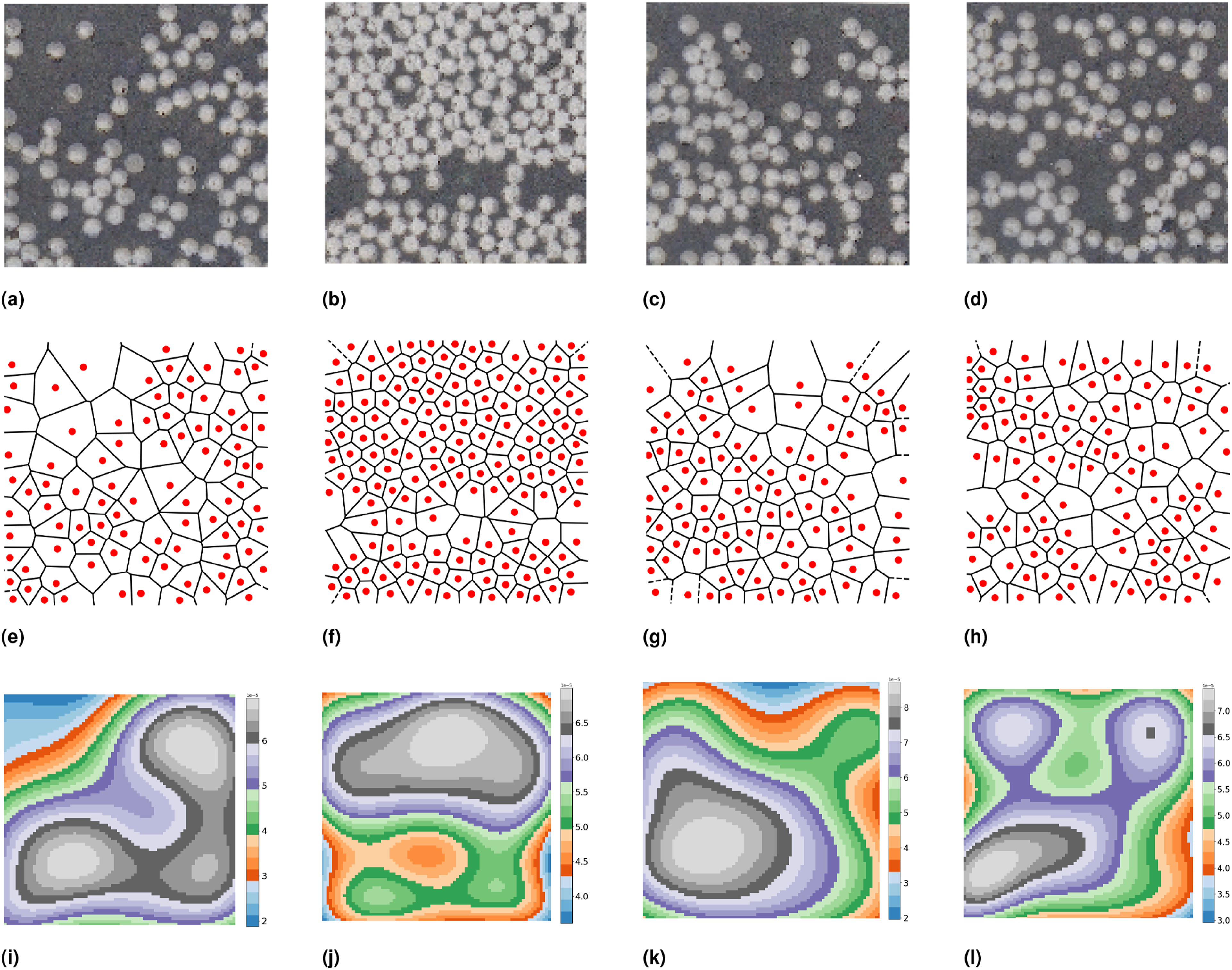

Kernel density function

In evaluating fiber distribution in a given domain, the Kernel Density Estimation (KDE) of a microscopy image involves estimating the probability density function of the pixel intensities associated with the fibers. KDE is a non-parametric method widely utilized in image segmentation, pattern recognition, and anomaly detection,^44,45 which can be computed for an image using equation (10). This study is used to identify the underlying density function of the fiber intensities, enabling the detection of not only the regions where fibers are tightly packed but also the number of peaks in the kernel density function revealing the number of high-fiber density regions and their spatial distribution.

K D E (x) = \frac{1}{n * h} * \sum K (\frac{x - x_{i}}{h})

(10)

Here the kernel density function of an image is computed with the number of pixels in the image(n), bandwidth also known as smoothing parameter(h), i^th pixel intensity, and Gaussian kernel function(K).

By applying KDE to the image, statistical parameters, such as the mean kernel density, can be derived, offering a quantitative assessment of the fiber distribution within the analyzed microstructure. Figure 11 presents various examples of microstructures with differing fiber distributions, alongside their corresponding KDE functions. The KDE accurately identifies regions with high fiber density, with peaks in the KDE indicating areas where fibers are closely packed. These densely packed regions are likely to contribute to stress concentration, thereby promoting the initiation and propagation of micro cracks.²⁰

Microstructure clustering based on fiber distribution

The results from the preceding machine learning step provide precise coordinates for all identified fibers, forming a fundamental basis for in-depth analysis of fiber distribution. From these coordinates, we extract critical quantitative descriptors such as Voronoi polygon areas, kernel density estimations, and fiber volume/area fractions. To effectively characterize various types within the microstructure, we employ higher-dimensional clustering techniques.

However, conventional clustering algorithms like K-means⁴⁶ often encounter computational challenges and diminished efficacy in high-dimensional spaces due to the curse of dimensionality, which complicates the definition of meaningful distances and the identification of significant clusters. To address these issues, we utilize advanced dimensionality reduction methods that transform complex, high-dimensional data into more manageable 2D and 3D representations. This transformation not only enhances clustering performance by mitigating computational constraints but also facilitates improved visualization and interpretation of microstructure types.

t-SNE for dimensionality reduction

t-SNE, which stands for t-distributed Stochastic Neighbor Embedding,⁴⁷ is a dimensionality reduction technique commonly used for visualizing high-dimensional data in lower dimensions while preserving the pairwise similarities between data points. In the presented work, it is employed for dimension reduction for pattern recognition applications using quantitative information from the Voronoi polygon, kernel density estimation, and fiber volume/area fraction.

p_{i | j} = \frac{e x p (\frac{- ‖ x_{i} - x_{j} ‖}{2 σ^{2}})}{\sum_{k \neq l} e x p (\frac{- ‖ x_{k} - x_{l} ‖}{2 σ^{2}})}

(11)

Q_{i j} = \frac{{[1 + ‖ y_{i} - y_{j} ‖]}^{- 1}}{\sum_{k \neq l} {[1 + ‖ y_{k} - y_{l} ‖^{2}]}^{- 1}}

(12)

P_{i j} = \frac{P_{i | j} + P_{j | i}}{2 N}

(13)

\frac{δ C}{δ y_{i}} = 4 \sum_{j} (p_{i j} - q_{i j}) (y_{i} - y_{j}) {(1 + ‖ y_{i} - y_{j} ‖^{2})}^{- 1}

(14)

The ultimate goal of this activity is to reduce the high dimensional data into comprehensible 2D and 3D, allowing us to use clustering algorithms effectively to identify the underlying microstructure patterns, and also suitable for visualization.

Microstructure categorizing using K-means

K-means is a popular clustering algorithm that divides a dataset into a specified number of clusters. It aims to minimize the sum of squared distances between data points and their respective cluster centers. In the presented work, it plays a crucial role in categorizing the microstructure based on fiber packing. It partitions the data into distinct clusters, enabling us to identify and analyze different fiber patterns within the composite material. The transformed data from t-SNE into 2D and 3D are subsequently used for identifying the distinct categories of microstructure with different fiber patterns. This transformation enhances the categorizing quality and provides clearer visual insights, making it an integral component of our analysis.

Initially, cluster centroids are randomly placed in the data space. Through iterative steps, each data point is assigned to the nearest centroid based on Euclidean distance, forming clusters using equation (15).

Assignment = {argmin}_{j} ‖ x_{i} - μ_{j} ‖^{2}

(15)

Where x_i is the data instance, μ_j is the centroid of a cluster j.

μ_{j} = \frac{1}{n_{j}} \sum_{i = 1}^{n} z_{i j} x_{i}

(16)

Here n_j is the number of the data instances in a given cluster j. z_ij is an indicator variable that equals to 1 if x_i is assigned to the cluster j, and 0 otherwise.

J = \sum_{i = 1}^{n} \sum_{j = 1}^{K} z_{i j} ‖ x_{i} - μ_{j} ‖^{2}

(17)

The centroids are then recalculated by averaging the data points within each cluster. This assignment-update cycle continues until convergence, usually when centroid positions stabilize or a predefined number of iterations is reached. K-means minimizes the sum of squared distances between data points and their respective centroids, effectively grouping similar data points.

The simplicity and efficiency of K-means clustering make it well-suited for this application, enabling effective categorization of microstructures based on fiber packing and dispersion. Each cluster formed by K-means reveals a distinct fiber distribution pattern, with differences highlighted by variations in the gaps between fibers and regions where fibers are densely packed.

Results and discussion

This section takes a detailed look at the results and conclusions from the methods described in section 3. The machine learning framework used to detect fibers is tested with advanced techniques, and the results are carefully analyzed and discussed.

Machine learning model evaluation

The machine learning framework detailed in Section 3 effectively detects fibers within a given microstructure. However, it is equally crucial to assess the accuracy of the trained models. In classification machine learning models, conducting post-hoc analysis on the trained model is essential. For this purpose, a testing dataset, unseen by the model during training, is employed to evaluate the model’s performance based on accurate and erroneous fiber pixel identifications. In this section, we introduce and provide a detailed explanation of the results obtained using various post-hoc methods, including the confusion matrix (CM) and receiver operator characteristics (ROC).⁴⁸ These methods offer valuable insights into the model’s classification performance and ability to distinguish between fiber and non-fiber regions within the microstructure.

There are several metrics to evaluate the performance of the trained model, like root mean square error used by,⁴⁹ and Mean Absolute Error (MAE) used by⁵⁰ for evaluating the model to predict the tensile strength of polymer/ CNTs nanocomposites. However the methods used in the present work like CM and ROC are more suited for classification based model.

In the second phase of our framework, an unsupervised machine-learning model is utilized to group fiber pixels into distinct clusters/fibers. The evaluation of this clustering process employs the Silhouette score, which prioritizes the creation of dense and well-separated clusters representing distinct fiber distribution patterns.

Classification model analysis

A CM is a tabular representation of the performance of a classification model that shows the predicted and actual labels for a data set. It provides a comprehensive summary of the model’s predictions and their agreement with the ground truth hand-labeled dataset. The confusion matrix consists of four main components: true positives (TP), true negatives (TN), false positives (FP), and false negatives (FN).

The FP and FN errors represent the type-1 and type-2 errors in statistics, respectively. In a standard CM, a strong diagonal suggests improved ML model performance on the test data. In Figure 12(a), diagonal members represent the instances when the model predicted the class correctly, and off-diagonal values represent the miss-classified data instances.

Figure 12.

Confusion matrix and receiver operator charactersitics for XGB model trained to detect fiber pixels from the bulk. (a) Confusion matrix (b) Receiver operator characteristics.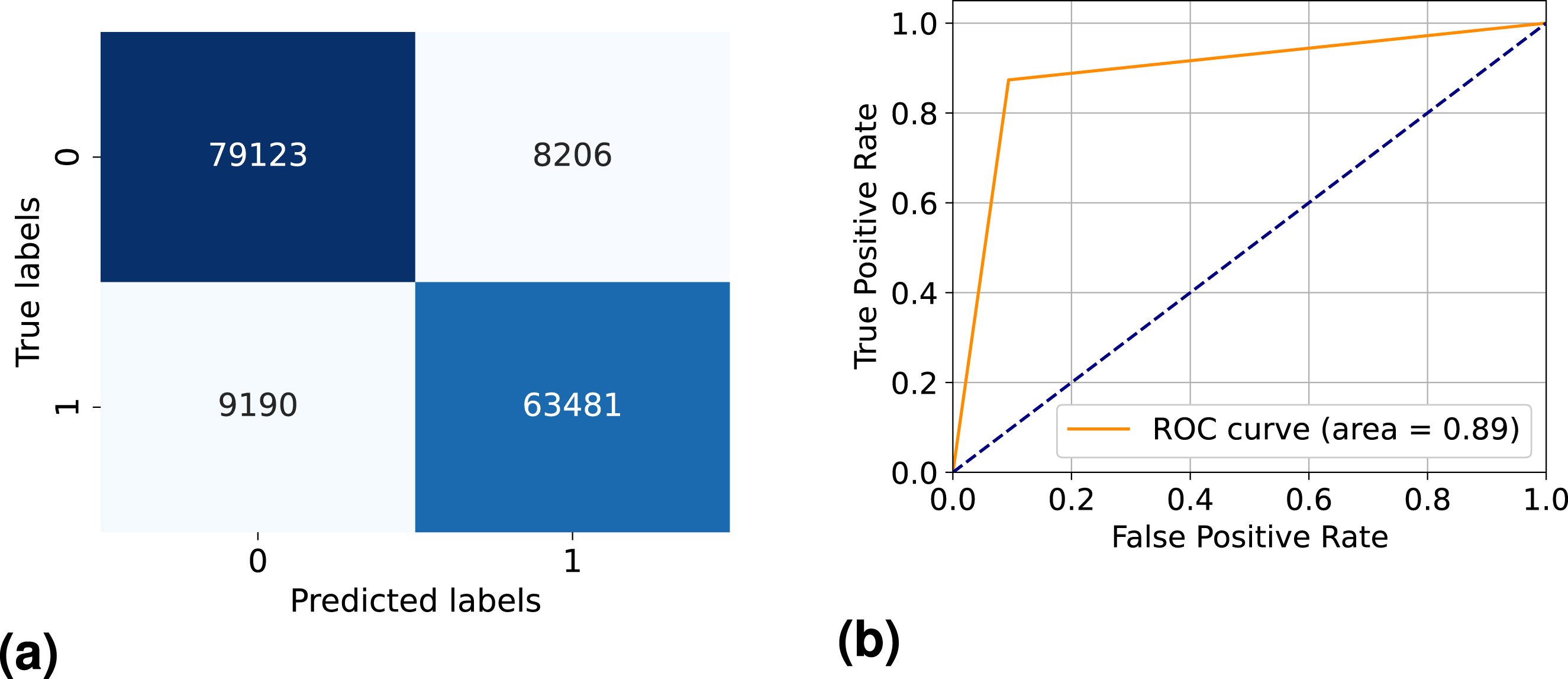

For a successfully trained model, a CM with a strong diagonal indicates that the model’s predictions align well with the ground truth labels. This diagonal dominance signifies accurate classification across various classes, showcasing the model’s proficiency in making correct predictions.

However, relying solely on the diagonal of the CM as a metric for model evaluation is inadequate. Therefore, based on the components of the CM true positives, true negatives, false positives, and false negatives, several metrics can be derived to comprehensively evaluate the performance of a classification model.

Indeed, different metrics obtained from the elements of the confusion matrix, such as precision (equation (18)) 0.88, recall (equation (19)) 0.87 and F1-Score (equation (20)) 0.88,⁵¹ were adopted:

P r e c i s i o n = \frac{T P}{T P + F P}

(18)

R e c a l l = \frac{T P}{T P + F N}

(19)

F 1_{Score} = 2 * \frac{P r e c i s i o n * R e c a l l}{P r e c i s i o n + R e c a l l}

(20)

The higher values of these derived units from the confusion matrix advocate for the better-performing model, showcasing its ability to accurately classify fiber pixels from the bulk.

The AUC-ROC is a metric commonly used for binary classification problems. It represents the area under the ROC curve, which plots the true positive rate (recall) against the false positive rate.

In this study, the model achieved an AUC score of 0.89 (see Figure 12(b)), demonstrating its effectiveness in distinguishing between fiber and matrix pixels using VGG16 features. This indicates that the model performed well, accurately identifying true positives while keeping false positives low.

Clustering evaluation

The Silhouette score⁵² is a metric commonly used to evaluate the quality of clusters produced by unsupervised machine learning algorithms, DBSCAN in the presented case. It provides a measure of how well-separated the clusters are and how similar the data points within the same cluster are to each other compared to data points in other clusters. The Silhouette score ranges from −1 to 1, where 1 represents that the data point is well matched to its cluster and poorly matched to neighboring clusters, while a score close to −1 indicates that the data point may have been assigned to the wrong cluster.

In the presented work, the Silhouette score is used to assess the quality of clustering performed to create distinct clusters from fiber pixels with an average score of 0.98. A visual representation of clusters from DBSCAN is shown in Figure 13(b).

Figure 13.

A figure depicting the results from DBSCAN clustering. (a) Prediction form XGB (b) Clustering from DBSCAN.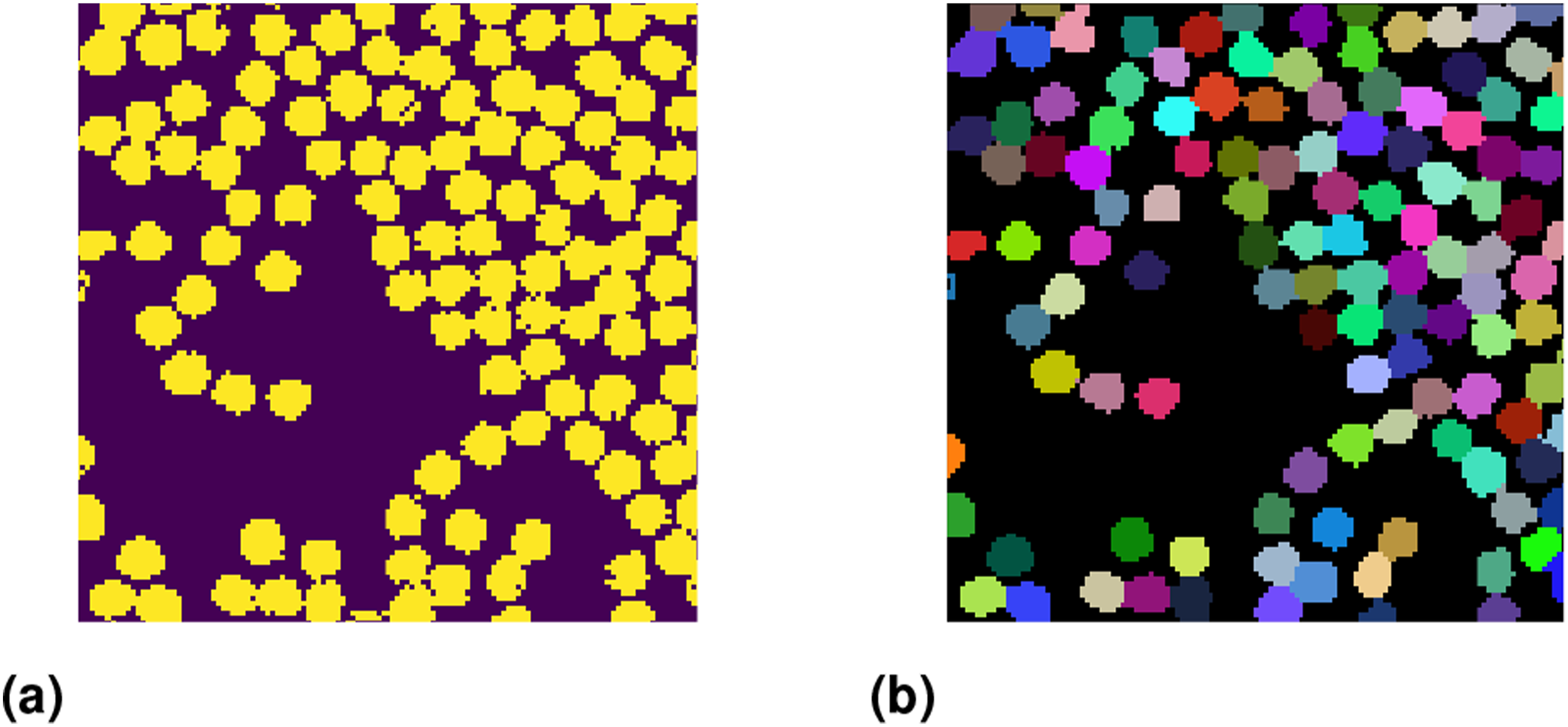

Comparison of fiber volume fraction

In section 2.3, a comprehensive method was employed to determine the FVF experimentally. Similar information can be deduced using the results from the presented machine learning framework.

Fiber volume fraction can be readily computed using microstructure image analysis using XGB segmentation. The pixels in the microstructure image are classified as fiber pixels and total pixels in the microstructure can be used as equation (9) for FVF evaluation.

In this work, in total 66969 microstructure images with three different scales are analyzed to obtain the overall FVF with a mean of 0.589 see Table 2 with a standard deviation within different scales equals to 1.583. A quantitative analysis of FVF in all the microstructure images in all three scales is depicted in Figure 14. It can be deduced that the results from the area fraction method are in alignment with results from Table 1.

Table 2.

Fiber volume fraction analysis on micro-strcture.

	25 μm	50 μm	125 μm
No.	47,477	18,056	1,396
Mean	0.612	0.577	0.58
Std	0.148	0.11	0.088

Figure 14.

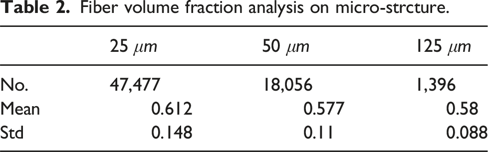
Fiber volume fraction analysis using microstructure images: (a) Fiber volume fraction distribution for 25 μm, (b) Fiber volume fraction distribution for 50 μm, and (c) Fiber volume fraction distribution for 125 μm.

The FVF obtained from the proposed method (0.589) and the TGV (0.59) analysis closely matches the material’s datasheet, demonstrating the method’s high accuracy. The FVF of the analyzed specimens falls within the expected range, meaning the fiber distribution did not significantly impact the material’s behavior at the macro level but had a notable influence on its micro-level behavior.^15,20

Evaluation for homogeneity based quantification

Results of voronoi polygon

The statistical analysis of polygon areas offers valuable insights into the spatial arrangement and uniformity of fibers within composite laminates. A smaller mean polygon area serves as an indicator of a more uniform and desirable distribution, signifying that each fiber occupies a consistent and well-defined space. Conversely, a larger mean polygon area suggests uneven spacing and clustering of fibers, potentially leading to structural vulnerabilities and diminished mechanical performance as described in Ref. 53.

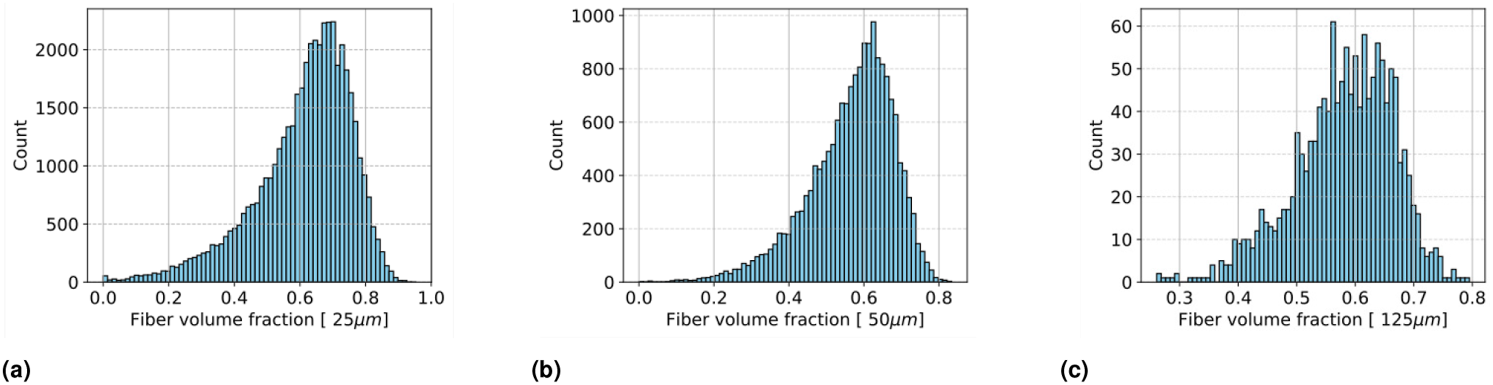
In Figure 15(d), a microstructure of 125 μm is shown with its Voronoi polygon representation Figure 15(f). It can be deduced that the fiber is close to evenly spaced represented by similar-sized polygons as shown in Figure 15(c).

Figure 15.

Voronoi polygon analysis, (a) Cell size 125μ m with low fiber count (d) Cell size 125μ m with high fiber count (g) Cell size 125μ m with medium fiber count ;(b) Voronoi polygon representation of low fiber count (e) Voronoi polygon representation of high fiber count (h) Voronoi polygon representation of medium fiber count; and (c) Polygon area distribution for low fiber count (f) Polygon area distribution for high fiber count (i) Polygon area distribution for medium fiber count.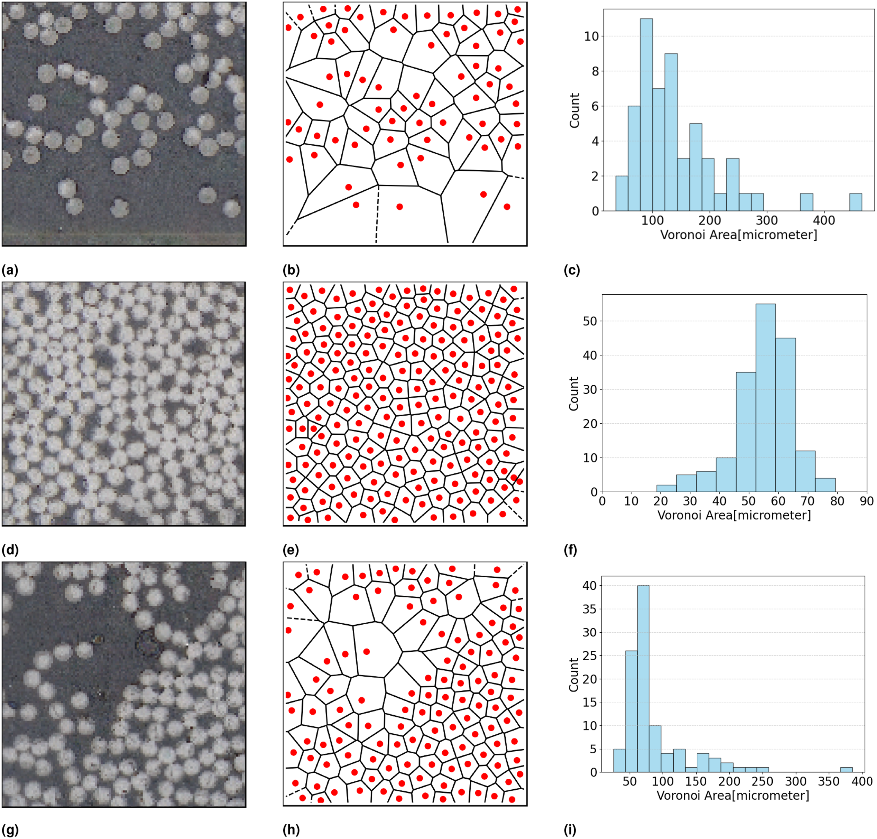

Other statistical characteristics reveal further information regarding the microstructure using Voronoi polygon areas. The smaller mean Voronoi area, see Figure 15(f) 55.54 μm, represents the tightly packed fiber arrangement in the given microstructure. Conversely, the higher mean Voronoi polygon area 141.04 μm represents the larger gaps as in Figure 15(c). Moreover, additional statistical measures, such as the standard deviation of Voronoi polygon areas, reveal the extent of variance in gaps between the fibers.

Further, higher-order statistics, including skewness and kurtosis, provide a deeper understanding of the distribution. Skewness assists in identifying whether the domain features more areas with tight fiber arrangement areas (left-skewed) with a few isolated less fiber regions as in Figure 15(c) or fewer such areas (right-skewed) as in Figure 15(f). Furthermore, kurtosis characterizes the tail of the Voronoi polygon areas. Higher kurtosis indicates a heavier tail, signifying a higher number of outlier sparse regions with very few fibers. Such regions are responsible for a possible increased rate of permeation.²²

Results of kernel density function

Similarly, a thorough statistical analysis of the kernel density estimation function may reveal deeper insights into the fiber packing. For instance, higher kernel density estimation infers regions with higher fiber density, and vice versa. It also reveals the number of peaks signifying the number of regions where the fibers are tightly packed.

As shown in Figure 16, 2D kernel density estimation of three different microstructures with their 1D distribution are shown. The mean and standard deviation of such function tell us about the high fiber density areas. Furthermore, exploring additional statistics, such as the standard deviation of the KDE, reveals variations in fiber density across the examined domain. Higher-order statistics, such as skewness and kurtosis, provide deeper insights into the distribution.

Figure 16.

(a) Original microstructure image with low fiber count;(d) Original microstructure image with high fiber count;(g) Original microstructure image with medium fiber count;(b) kernel density representation with low fiber count;(e) kernel density representation with high fiber count;(e) kernel density representation with medium fiber count;(c) kernel density distribution with low fiber count;(f) kernel density distribution with high fiber count;(i) kernel density distribution with medium fiber count.

Skewness is particularly useful in determining the symmetry of fiber distribution. For example, a right-skewed distribution indicates a higher concentration of fibers in certain areas, which could lead to localized stress concentrations.²¹ Conversely, a left-skewed distribution suggests that such areas are sparse.

Additionally, kurtosis characterizes the tail of the KDE. Higher kurtosis value implies that there are more extreme outliers regions of abnormally high fiber density with are potential to create nucleation sites for matrix cracking.⁴³

Dimensionality reduction and clustering

The micro-section images are cropped into smaller domains of different sizes, which are analyzed by the VGG16, XGB, and DBSCAN models to detect the fibers. The spatial distribution of the fibers is analyzed using statistical analysis like Voronoi polygon and kernel density estimation.

Spatial statistical analysis like Voronoi polygon area statistics and kernel density analysis provides extensive information regarding the fiber distribution pattern. Further, to circumvent the rotational invariant property of microstructure, area moment of inertia was employed. These statistics together with the fiber volume fraction sum up to 9 (4-Voronoi polygon statistics; 4-KDE statistics; and FVF) features representing a microstructure.

In higher-dimensional feature spaces, such as the 9-dimensional space representing microstructures, the complexity of the data increases, and it becomes challenging to visualize and interpret meaningful patterns directly. Clustering algorithms like K-means struggle with high-dimensional data due to the curse of dimensionality,⁵⁴ where distances between points become less meaningful as the number of dimensions increases.

To circumvent this issue and facilitate the clustering of microstructures, the dimensionality reduction method, t-SNE, is used for visualizing high-dimensional data in lower-dimensional spaces while preserving local structures and capturing non-linear relationships, which will be used to draw meaningful patterns in the microstructure.

Results of t-SNE

t-SNE is a dimensionality reduction technique, traditionally used for visualizing high dimensional data^55,56 in lower dimensions while preserving the pairwise similarities between data points.

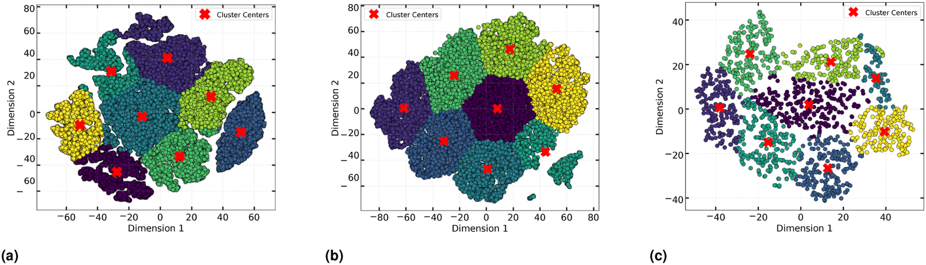
A 2D t-SNE dimensional representation is shown in Figure 17. Each point in this distribution represents a distinct microstructure. All such points are analyzed using K-means to create distinct clusters. Different colors represent the distinct clusters with cluster centers marked as red crosses. A similar analysis was conducted on microstructures of varying sizes, specifically those with dimensions of 125 μm, 50 μm, and 25 μm (see Figure 18).

Figure 17.

2D t-SNE representation with 8 clusters using K-means, with one example shown from few clusters.

Figure 18.

2D dimensionality reduction using t-SNE and K-means clustering results, (a) 25 μm ,(b) 50 μm, and (c) 125 μm.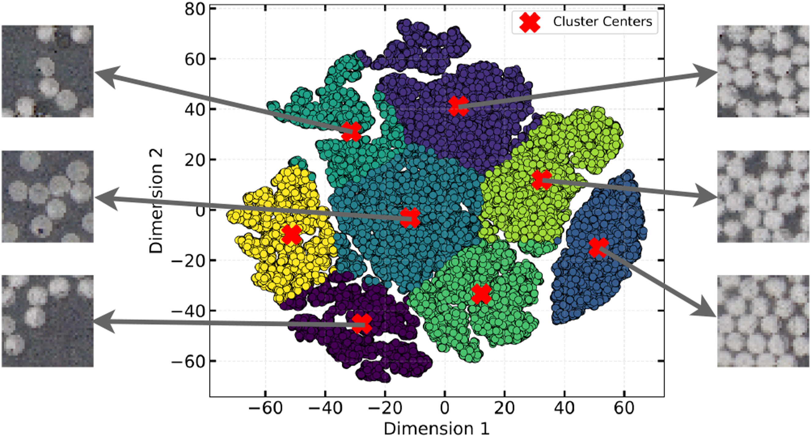

For better comprehensibility of the clusters, t-SNE representation of the microstructures was also performed in 3D. Analogously in 3D as well, K-means was used to group the different microstructures into distinct clusters, which are represented with various colors in Figure 19.

Figure 19.

3D t-SNE representation with 6 clusters using K-means for all the 3 cell sizes; (a) 125 μm, (b) 50 μm, (c) 25 μm.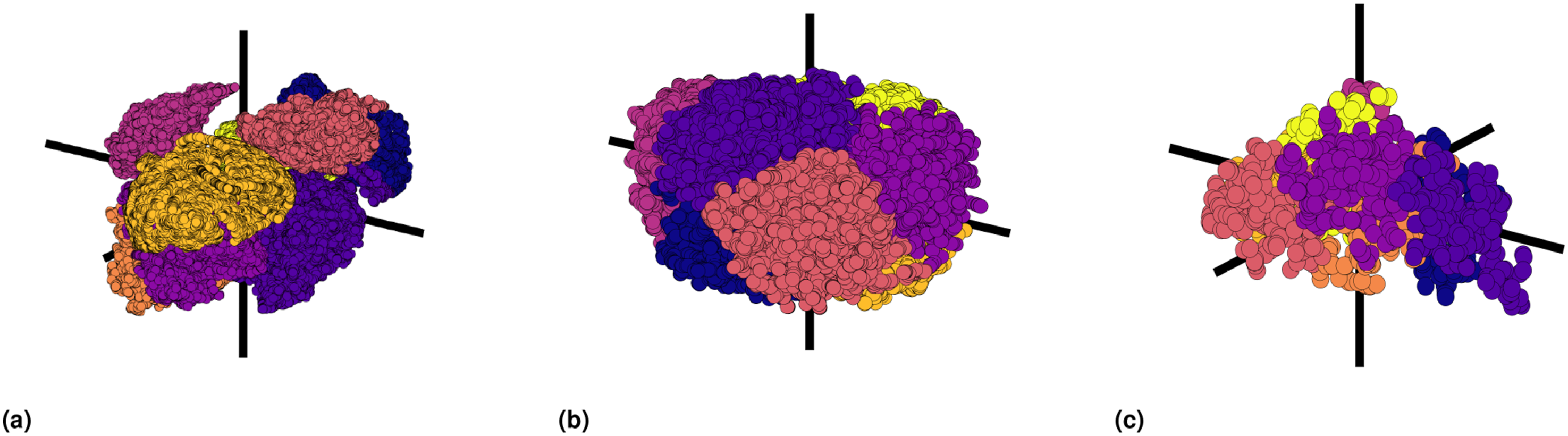

Results on K-means

Following dimensionality reduction, K-means clustering was applied to both the 2D and 3D datasets. However, K-means requires the value ”k (number of clusters)” apriori to create clusters. This crucial task of determining the optimal number of clusters (k) was performed by employing a well-known method termed an ”elbow plot”. It involved executing the k-means algorithm for a range of cluster numbers and plotting the within-cluster sum of squares (Equation (17)) against the number of clusters. The ”elbow point”, where the rate of decrease in the within-cluster sum of squares slows down, was identified as the optimal number of clusters. Later the ”k” at the elbow point was employed again to perform the final clustering. This process was repeated for both the dimensions (2D and 3D ) across three domain sizes 125 μm, 50 μm, and 25 μm. The elbow plots for this experiment are shown in Figure 20.

Figure 20.

A figure depicting the results from DBSCAN clustering. (a) Normalized elbow plot for 2D with 25 μm, 40 μm, and 125 μm, (b) Normalized elbow plot for 3D with 25 μm, 40 μm, and 125 μm.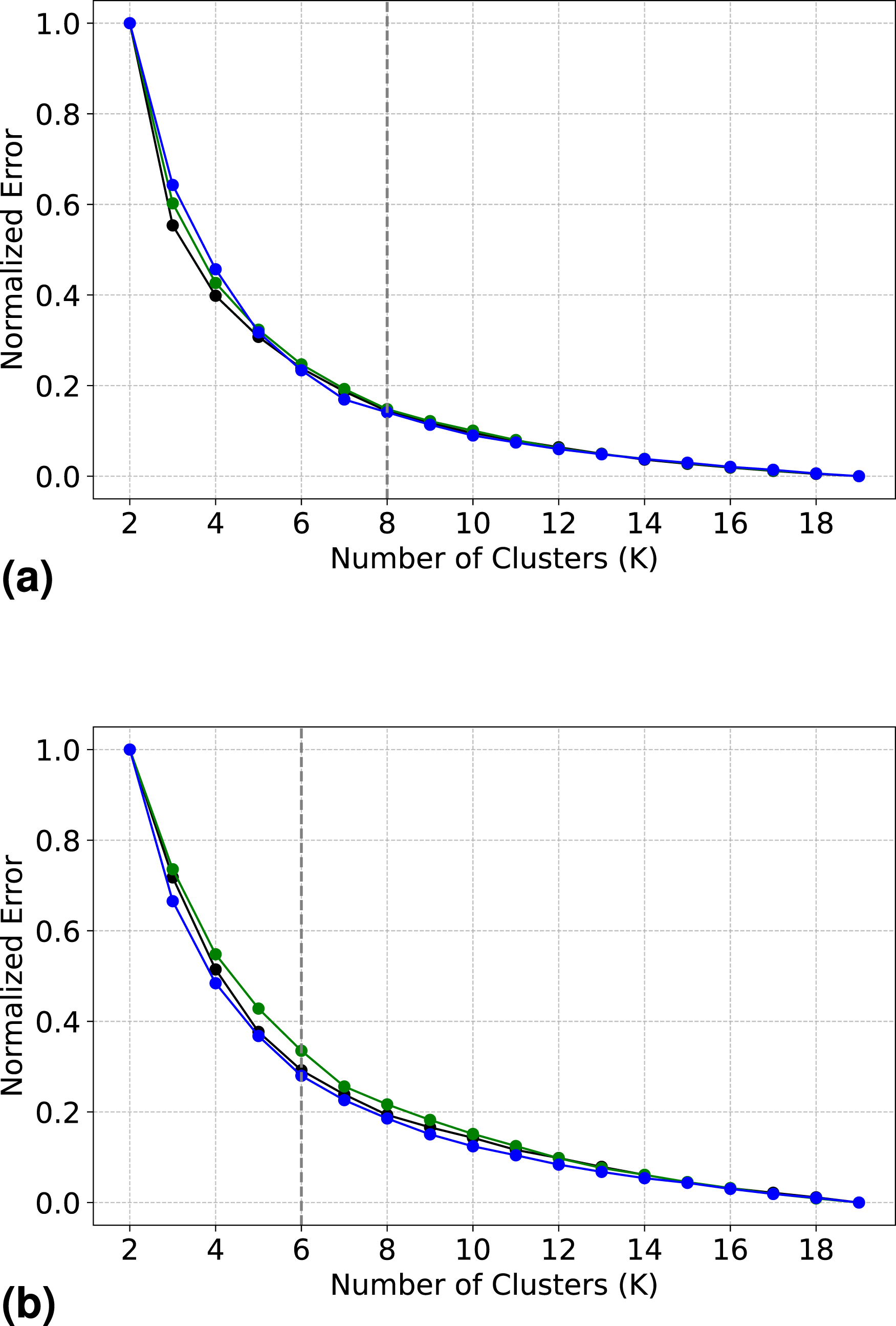

This process results in a finite number of distinct microstructure types within the laminate, defined based on features extracted from microsection images. These features, such as Voronoi area, KDE, and FVF, enable us to categorize different microstructures and help us to understand the fiber packing patterns.

These classifications are not just useful for characterizing the micro-level behavior of the material; they also play a key role in multiscale simulations. In such simulations, these distinct microstructure may be used as RVEs to model the material’s behavior across different scales—from the microscopic interactions between fibers and matrix to the macroscopic response of the entire laminate.

Explainability using surrogate model

AI has become a powerful asset in materials science, enabling fast and accurate predictions of key material properties such as electronic, magnetic, and elastic characteristics, as well as formation energy and band gaps.⁵⁷ This capability allows for the efficient screening of vast material search spaces to identify candidates with desirable properties. Deep learning models, including graph neural networks, capture complex structure-property relationships directly from data, enhancing predictive accuracy. Moreover, AI accelerates the discovery and design of novel materials by uncovering critical structural and chemical features, offering a data-driven approach to materials informatics. In this rapidly advancing field, XAI is increasingly essential to ensure the reliability, interpretability, and trustworthiness of AI-driven predictions.^58,59

Post-hoc analysis of a machine learning model may offer insights into its performance on a specific dataset, but it often lacks interpretability regarding individual predictions. Additionally, challenges such as data incompleteness, lack of representation, and data leakage—where training data may inadvertently leak into the testing set—can further complicate analysis.

Therefore, it becomes crucial to understand ”why a model makes a specific prediction”, providing insights into its decision-making process and inner workings. Explainability serves to instill ”Trust”, ”Accountability”, and ”Bias Identification” in the model’s predictions.⁶⁰

Surrogate model

In the intricate process of micro-section clustering, we leverage the non-linear dimensionality reduction technique t-SNE, followed by K-means clustering, to derive meaningful patterns. The complexity of this approach poses challenges for conventional XAI frameworks for interpretability, which can be defined as the ability to trust a prediction and ultimately trust a model.

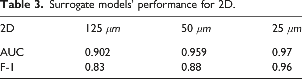
Therefore to circumvent these challenges, we adopt a surrogate model to serve as a bridge between the non-linear clustering step and interpretability. This surrogate model, based on the XGBoost algorithm introduced in Section 3, maps the clustering results obtained in the reduced dimensionality space to their higher-dimensional counterparts. This two-step approach not only facilitates the interpretation of the clustering outcomes but also enhances the overall understanding of the intricate relationship between features and microstructure types across varying dimensions (Table 3).

Table 3.

Surrogate models’ performance for 2D.

2D	125 μm	50 μm	25 μm
AUC	0.902	0.959	0.97
F-1	0.83	0.88	0.96

Similar testing and verification methods mentioned in Section 3 were employed to obtain the average AUC score of 0.951, and F-1 Score are shown in Table 4. This infers that the surrogate models are trained well to predict the microstructure types and effectively map features to clusters.

Table 4.

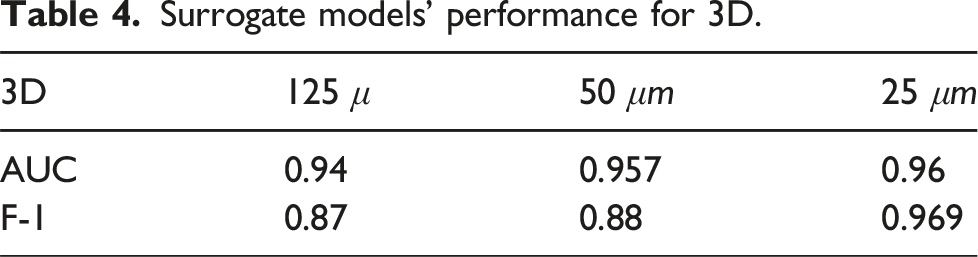
Surrogate models’ performance for 3D.

3D	125 μ	50 μm	25 μm
AUC	0.94	0.957	0.96
F-1	0.87	0.88	0.969

SHapley additive exPlanations for model explainability

Model explainability has become a vital focus in machine learning research, driven by the increasing need to understand and trust the decisions made by complex, often opaque models. To address this challenge, various interpretability techniques have been developed, including model agnostic methods such as SHAP (SHapley Additive Explanations)^60,61 and LIME (Local Interpretable Model-Agnostic Explanations),⁶² as well as inherently interpretable models like decision trees and linear regression.⁶³ In parallel, advancements in deep learning interpretability such as feature visualization and attention mechanisms⁶⁴ have contributed to a better understanding of neural networks and other black-box models.

Recent studies have applied XAI tools, particularly SHAP, to enhance interpretability in material science and structural engineering contexts. For instance, Ke et al.⁶⁵ utilized SHAP to interpret the predictions of a CatBoost model for CFRP–steel epoxy bond strength, enabling a quantitative understanding of each feature’s contribution to model outputs and thereby simplifying the decision-making process. Similarly, Yossef et al.⁶⁶ employed SHAP to analyze the influence of material properties such as E₁, E₂, G₁₂, G₂₃, and v₁₂ on composite strength, identifying the longitudinal modulus (E₁) as the most critical feature. In another application, Zhao et al.⁶⁷ used SHAP to interpret an XGBoost model predicting Compression-After-Impact (CAI) strength in carbon/glass hybrid laminates. Their SHAP-based analysis quantified the effect of impact parameters and revealed the complex, non-linear relationships.

These studies demonstrate the growing utility of SHAP in revealing the inner workings of machine learning models applied to composite material systems, offering domain experts a transparent pathway to interpret predictions and extract physically meaningful insights.

In the presented work, the inner workings of the surrogate model presented previously is explained using SHAP. The input features like kernel density enstimation, voronoi polygon statistics and fiber volume are correlated with micro-structure clustering by tSNE.

SHAP is based on cooperative game theory and provides a way to fairly distribute value among a group of contributors. In the context of model explainability, SHAP values assign a contribution to each feature in a prediction, indicating how much each feature contributes to the model’s output. For machine learning, each feature is considered a player, and the value to be distributed is the difference between the model’s output and the average output. The Shapley value of a feature is the average contribution of that feature to all possible combinations of features.

The SHAP method follows three conditions for interpretability. Firstly, the condition of Missingness dictates that the SHAP value of a missing feature is inherently assigned a value of zero. This ensures that the absence of a particular feature does not impart any contribution to the model’s output. Secondly, the principle of Additivity holds, compelling the model’s output to be the sum of the contributions from individual features. This additive property reinforces the interpretability of SHAP values, as the overall model prediction is comprehensively decomposed into the impact of each feature. Lastly, Consistency is maintained, signifying that if the marginal contribution of a feature increases or remains constant due to alterations in the model, the corresponding Shapley value will exhibit a corresponding increase or maintain its current level. These conditions collectively contribute to the reliability and interpretability of the SHAP method.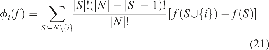

ϕ_{i} (f) = \sum_{S \subseteq N \ {i}} \frac{| S |! (| N | - | S | - 1)!}{| N |!} [f (S \cup {i}) - f (S)]

(21)

In equation (21),S ⊆ N \{i} represents all possible subsets S of the features in N excluding the feature i. |S| is cardinality ,number of elements, in subset S, and |N|: The total number of features. The global contribution of a feature can be calculated by averaging the shapely value for each feature in the dataset as in equation (22)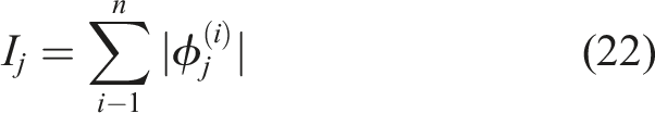

I_{j} = \sum_{i - 1}^{n} | ϕ_{j}^{(i)} |

(22)

Global interpretation of a machine learning model can be achieved through the analysis of feature importance, which offers insights into how each feature influences the model’s predictions. Using equation (22), we compute the contribution of each feature across different microstructure types, with the results visualized in Figure 21.

Figure 21.

Feature importance plots using SHAP values for different surrogate models. (a) Surrogate model for 2D mapping with 25 μm, (b) Surrogate model for 2D mapping with 50μm, (c) Surrogate model for 2D mapping with 125 μm, (d) Surrogate model for 3D mapping with 25 μm, (e) Surrogate model for 3D mapping with 50 μm, (f) Surrogate model for 3D mapping with 125 μm.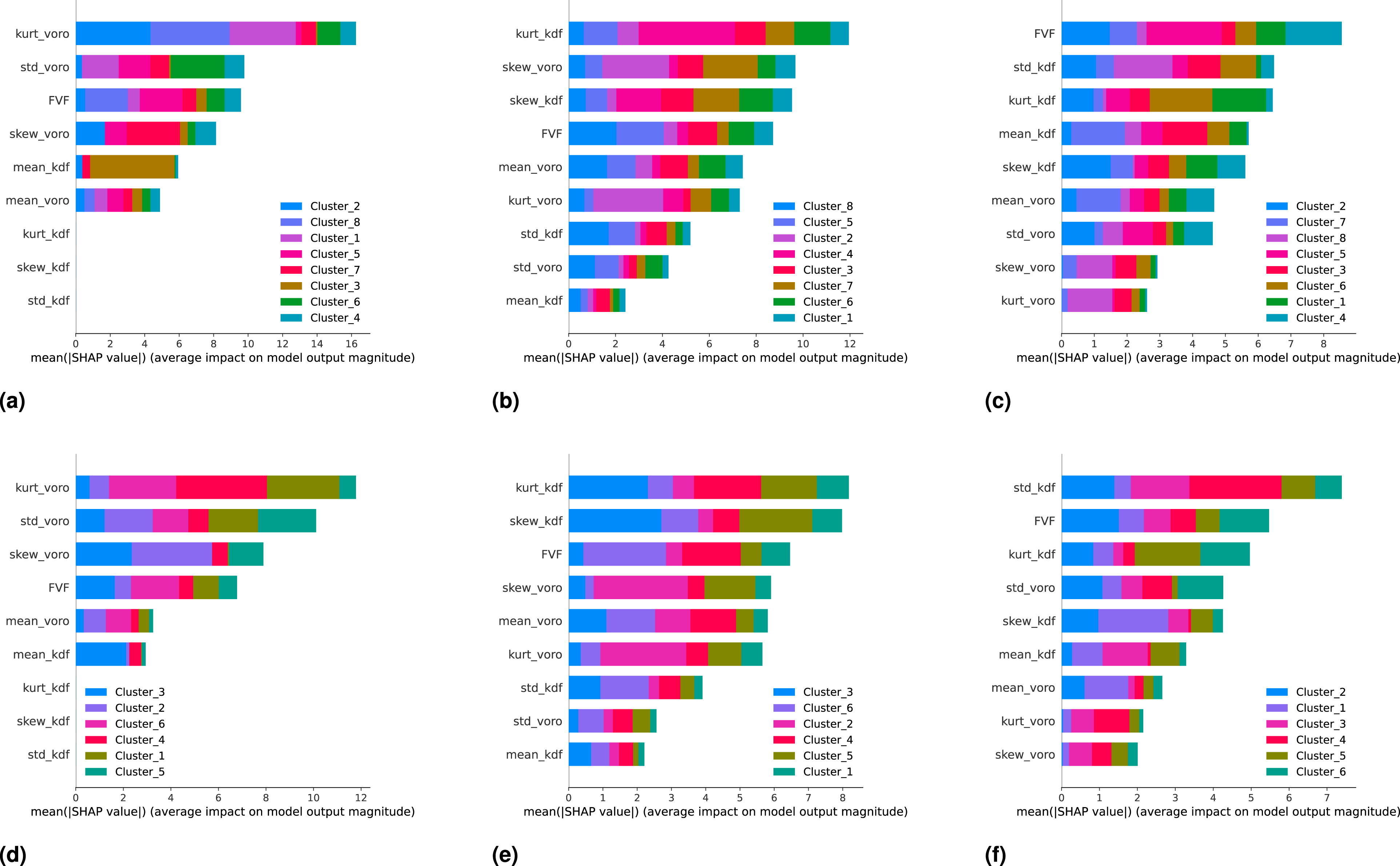

In this feature importance plot, features are ranked in descending order based on their contribution to the model’s predictions. The length of each bar indicates the strength of that contribution, while the colors represent the impact of the feature on specific microstructure classes. This plot provides not only a global overview of the model’s behavior but also reveals how individual features drive the classification of particular microstructure types.

From Figure 21, we observe that the top five contributing features kurtosis and standard deviation of Voronoi polygon areas, FVF, mean kernel density estimation , and mean Voronoi area, offer practical insights into the physical behavior of the microstructures. A high kurtosis of Voronoi areas suggests the presence of outlier regions with very large or very small fiber free zones, which are often linked to stress concentrations and early matrix cracking. Similarly, a high standard deviation implies uneven fiber spacing, resulting in local stiffness heterogeneity and potential zones of damage initiation. The FVF, as a direct measure of fiber content, pushes the classification toward denser microstructure clusters, typically associated with greater load bearing capacity. The mean KDE quantifies local fiber concentration; lower values may indicate loosely packed regions, which are relevant to resin rich zones and permeability. Finally, the mean Voronoi area complements the KDE by representing the average spacing between fibers larger values indicate sparser fiber networks. These interpretations enhance the physical understanding behind the SHAP based rankings and reinforce the surrogate model’s explainability.

As the domain size decreases, the relative importance of features such as KDE diminishes, as seen in Figure 21. This is due to the reduced likelihood of encountering fiber packing anomalies in smaller domains. While KDE effectively captures variations in fiber density in larger domains important for modeling stress concentrations and potential cracking these features become less distinguishable at smaller scales, reducing their influence on the classification outcome.

This shift in feature importance underscores a key limitation of using RVEs. Small RVEs often fail to capture critical microscale phenomena, such as fiber-matrix interactions and the initiation or propagation of matrix cracks.^27,28,68 In contrast, larger RVEs better represent these interactions and the spatial variability in fiber packing, thereby allowing more accurate modeling of mechanical behavior.

Conclusion and outlook

The paper introduces a data-driven approach to analyze and categorize microstructures, focusing on identifying key microstructural features using advance XAI methods and spatial statistics.

Using microstructure clustering, this study highlights distinct fiber distribution patterns, which are then correlated with failure phenomena such as permeation, matrix cracking, and crack propagation based on existing literature.

While this work primarily focuses on microstructural characterization, the insights gained could potentially aid in quality assurance for CFRP manufacturing.

Key points and findings from the paper can be summarized as follows:

• Existing methodologies for fiber detection and RVE generation for multi-scale approaches in CFRP are discussed, highlighting their limitations;

• A well-known DCNN, VGG16, is employed as a feature extractor to capture fiber distribution patterns from micro-section images. A hand-labeled mask, together with the extracted features, was used as training and testing data for a state-of-the-art tree-based model, XGB, to detect fibers in a given microstructure image with an accuracy of 89%;

• A sophisticated spatial clustering technique (DBSCAN) is employed to group fiber pixels into distinct fibers, and their coordinates were analyzed using advanced statistical techniques such as Voronoi polygon statistics and kernel density estimation to extract meaningful insights into fiber distribution;

• These statistical features together with FVF were further processed using dimensionality reduction (t-SNE) and clustering (K-means) to identify rational patterns and group similar microstructures;

• An XAI framework was implemented using the SHAP method, applied in the context of XGBoost-based surrogate models across different scales and dimensions;

• All trained surrogate models were evaluated using various ML model evaluation techniques, including confusion matrix, F-1 Score, and ROC curve analysis with AUC;

• The extracted microstructure patterns provide a basis for quality assurance in CFRP manufacturing by offering an automated method to detect irregularities in fiber distribution, which can impact mechanical performance. By identifying deviations from optimal fiber arrangements, this approach enables real-time monitoring and defect detection, ensuring consistency in production;

• These identified microstructure patterns also serve as a foundation for multiscale modeling, where representative microstructural clusters can be integrated into higher-scale simulations. This facilitates a more accurate prediction of material behavior at macro-scales by incorporating real-world microstructural variations;

While the proposed approach provides valuable insights, some limitations must be addressed. The reliance on hand-labeled masks introduces potential subjectivity, and the generalization of the models to other materials or imaging conditions requires further validation. Additionally, the clustering results are sensitive to parameter tuning in t-SNE, which may affect the robustness of the approach in different datasets. Lastly, though correlations between microstructure patterns and failure mechanisms are identified using existing literature, a quantitative validation of these relationships with experimental data and numerical simulations remains an area for further exploration.

By systematically addressing the complexities of microstructure patterns, this work contributes to the current state of knowledge in building micro-scale FE models. The data-driven and XAI approach used in this study not only enhances the understanding of microstructural behavior but also lays the groundwork for future research in integrating machine learning-driven microstructure characterization into multiscale modeling frameworks. A key next step is to utilize the identified RVE patterns in numerical simulations to establish correlations between spatial features and material properties. Additionally, this approach can be extended to a data-driven multiscale framework, enabling a more accurate representation of intricate failure phenomena and improving predictive modeling of composite materials

Footnotes

Acknowledgements

We acknowledge their support in making this research possible.

Declaration of conflicting interests

The author(s) declared no potential conflicts of interest with respect to the research, authorship, and/or publication of this article.

Funding

The author(s) disclosed receipt of the following financial support for the research, authorship, and/or publication of this article: Funding for this project was provided by the Federal Ministry for Economic Affairs and Climate Action of the Federal Republic of Germany (BMWK) under the project CryoCrack - Berechnungskonzept zur Bewertung der Bildung von Leckagenetzwerken in kryogenen CFK-Wasserstofftanks, Förderkennzeichen 50RL2230A.

ORCID iDs

Harsh Bordekar

Josef Koord

Oliver Völkerink

Christian Hühne

Data Availability Statement

Data sharing not applicable to this article as no datasets were generated or analyzed during the current study.

References

Schlapbach

Züttel

. Hydrogen-storage materials for mobile applications. Nature 2001; 414(6861): 353–358.

Rolo

Costa

VAF

Brito

. Hydrogen-based energy systems: current technology development status, opportunities and challenges. Energies 2023; 72(17): 1–180.

Balasooriya

Clute

Schrittesser

, et al. A review on applicability, limitations, and improvements of polymeric materials in high-pressure hydrogen gas atmospheres. Polym Rev 2022; 62(1): 175–209.

Azeem

Alam

; et al. Application of filament winding technology in composite pressure vessels and challenges: a review.

Air

Oromiehie

Prusty

. Design and manufacture of a type V composite pressure vessel using automated fibre placement. Compos B Eng 2023; 266: 111027.

Mallick

Cronin

Fabian

, et al. Microcrack resistant polymers enabling lightweight composite hydrogen storage vessels. In: Wicks

Simon

Zidan

, et al. (eds). Materials Challenges in Alternative and Renewable Energy, 2011, pp. 91–98.

Grogan

Ó Brádaigh

CMÓ

McGarry

, et al. Damage and permeability in tape-laid thermoplastic composite cryogenic tanks. Compos Appl Sci Manuf 2015; 78: 390–402.

Grimsley

Cano

Johnston

, et al. Hybrid composites for LH2 fuel tank structure.” 2001.

Huang

Jin

. Effects of fiber arrangement on mechanical behavior of unidirectional composites. J Compos Mater 2008; 42(18): 1851–1871.

10.

Vaughan

McCarthy

. Micromechanical modelling of the transverse damage behaviour in fibre reinforced composites. Compos Sci Technol 2011; 71(3): 388–396.

11.

Kaushik

Saikia

Bedi

, et al. Effect of fiber anisotropy and interphase on the stress jumps across the fiber/matrix interface in fuzzy fiber composites. Natl Acad Sci Lett 2023; 46(2): 165–171.

12.

Meng

Wang

Yang

, et al. Mechanical properties and internal microdefects evolution of carbon fiber reinforced polymer composites: cryogenic temperature and thermocycling effects. Compos Sci Technol 2020; 191: 108083.

13.

Yan

Liu

Jiang

, et al. Mechanism of matrix influencing the cryogenic mechanical property of carbon fibre reinforced epoxy resin composite. Compos Commun 2022; 33: 101220.

14.

Adams

Bowles

Herakovich

. Thermally induced transverse cracking in graphite-epoxy cross-ply laminates. J Reinforc Plast Compos 1986; 5(3): 152–169.

15.

Mital

Gyekenyesi

Arnold

, et al. (2006). Review of current state of the art and key design issues with potential solutions for liquid hydrogen cryogenic storage tank structures for aircraft applications.

16.

Meng

Zheng

Wei

, et al. Leakage performance of CFRP laminate under cryogenic temperature: experimental and simulation study. Compos Sci Technol 2022; 226: 109550.

17.

Kumazawa

Ishikawa

Suzuki

, et al. Modeling of propellant leakage through matrix cracks in composite laminates. In: 19th AIAA applied aerodynamics conference, 2001, p. 1217.

18.

Hamori

Kumazawa

Higuchi

, et al. Gas permeability of CFRP cross-ply laminates with thin-ply barrier layers under cryogenic and biaxial loading conditions. Compos Struct 2020; 245: 112326.

19.

Nair

Roy

. Modeling of permeation and damage in graphite/epoxy laminates for cryogenic tanks in the presence of delaminations and stitch cracks. Compos Sci Technol 2007; 67(11-12): 2592–2605.

20.

Cater

Xiao

Goldberg

, et al. Multiscale investigation of micro-scale stresses at composite laminate free edge. Compos Struct 2018; 189: 545–552.

21.

González

Llorca

. Mechanical behavior of unidirectional fiber-reinforced polymers under transverse compression: microscopic mechanisms and modeling. Compos Sci Technol 2007; 67(13): 2795–2806.

22.

Ebermann

Bogenfeld

Kreikemeier

, et al. Analytical and numerical approach to determine effective diffusion coefficients for composite pressure vessels. Compos Struct 2022; 291: 115616.

23.

Kim

Lim

Lee

. Prediction and validation of the transverse mechanical behavior of unidirectional composites considering interfacial debonding through convolutional neural networks. Compos B Eng 2021; 225: 109314.

24.

Wang

, et al. Damage behaviors of unidirectional CFRP in orthogonal cutting: a comparison between single- and multiple-pass strategies. Compos B Eng 2020; 185: 107774.

25.

Okereke

Akpoyomare

. A virtual framework for prediction of full-field elastic response of unidirectional composites. Comput Mater Sci 2013; 70: 82–99.

26.

Liu

Zhu

. Generation of random fiber distributions for unidirectional fiber‐reinforced composites based on particle swarm optimizer. Polym Compos 2019; 40(4): 1643–1653.

27.

Herráez

Segurado

González

, et al. A microstructures generation tool for virtual ply property screening of hybrid composites with high volume fractions of non-circular fibers - viper. Compos Appl Sci Manuf 2020; 129: 105691.

28.

Wang

Dai

Zhang

, et al. Micromechanical modeling of fiber-reinforced composites with statistically equivalent random fiber distribution. Materials 2016; 9(8): 624.

29.

Saito

Takeuchi

Kimpara

. Experimental evaluation of the damage growth restraining in 90° layer of thin-ply CFRP cross-ply laminates. Adv Compos Mater 2012; 21(1): 57–66.

30.

Seuffert

Bittrich

Cardoso de Oliveira

, et al. Micro-scale permeability characterization of carbon fiber composites using micrograph volume elements. Frontiers in Materials 2021; 8: 745084.

31.

Zhang

. Predicting the delamination factor in carbon fibre reinforced plastic composites during drilling through the Gaussian process regression. J Cell Plast. 2021; 55(15): 2061–2068.

32.

Zhang

. Predicting mechanical performance of starch-based foam materials. J Cell Plast 2022; 58: 505–514.

33.

Tkachenko

Malyuk

Holmanyuk

, et al. Label studio: data labeling software. 2020. https://github.com/heartexlabs/label-studio

34.

Yuen

Princen

Illingworth

, et al. Comparative study of Hough transform methods for circle finding. Image Vis Comput 1990; 8(1): 71–77.

35.

Simonyan

Zisserman

. Very deep convolutional networks for large-scale image recognition. arXiv preprint arXiv:1409.1556, 2014.

36.

Deng

Dong

Socher

, et al. ImageNet: a large-scale hierarchical image database. 2009 IEEE conference on computer vision and pattern recognition, 2009, pp. 248–255.

37.

Chen

Guestrin

. XGBoost. Proceedings of the 22nd ACM SIGKDD International Conference on Knowledge Discovery and Data Mining 2016: 785–794.

38.

Ester

Kriegel

Sander

, et al. A density-based algorithm for discovering clusters in large spatial databases with noise. Kdd 1996; 96(34): 226–231.

39.

Wang

Sun

, et al. An efficient method to generate random distribution of fibers in continuous fiber reinforced composites. Polym Compos 2019; 40(12): 4763–4770.

40.

Wkeglarczyk

. Kernel density estimation and its application. In: ITM web of conferences. EDP Sciences, 2018, vol 23, p. 00037.

41.

Sharifpour

Bahmani

, et al. A new approach to rapidly generate random periodic representative volume elements for microstructural assessment of high volume fraction composites. Mater Des 2018; 150: 124–138.

42.

Ahn

. Voronoi diagrams for a moderate-sized point-set in a simple polygon. arXiv, 2018, eprint 1801.02292, archivePrefix arXiv, primaryClass cs.CG.

43.

Herráez

Mora

Naya

, et al. Transverse cracking of cross-ply laminates: a computational micromechanics perspective. Compos Sci Technol 2015; 110: 196–204.

44.

Baccar

Söffker

. Identification and classification of failure modes in laminated composites by using a multivariate statistical analysis of wavelet coefficients. Mech Syst Signal Process 2017; 96: 77–87.

45.

Phillips

Anderson

Schapire

. Maximum entropy modeling of species geographic distributions. Ecol Model 2006; 190(3-4): 231–259.

46.

Arthur

Vassilvitskii

. k-means++: the advantages of careful seeding. Soda 2007; 7: 1027–1035.

47.

Van der Maaten

Hinton

. Visualizing data using t-SNE. J Mach Learn Res. 2008; 9(11): 2589–2605.

48.

Mandrekar

. Receiver operating characteristic curve in diagnostic test assessment. J Thorac Oncol 2010; 5(9): 1315–1316.

49.

Jin

. Wholesale price forecasts of green grams using the neural network. Asian journal of economics and banking. Emerald Publishing Limited, 2024.

50.

. Prediction of tensile strength of polymer carbon nanotube composites using practical machine learning method. J Compos Mater 2021; 55(6): 787–811.

51.

Fawcett

. An introduction to ROC analysis. Pattern Recognit Lett 2006; 27(8): 861–874.

52.

Shahapure

Nicholas

. Cluster quality analysis using silhouette score. In: 2020 IEEE 7th international conference on data science and advanced analytics (DSAA). IEEE, 2020, pp. 747–748.

53.

McMains

. A Voronoi diagram approach for detecting defects in 3D printed fiber-reinforced polymers from microscope images. Computational Visual Media 2023; 9(1): 41–56.

54.

Verleysen

François

. The curse of dimensionality in data mining and time series prediction. In: International work-conference on artificial neural networks. Springer, 2005, pp. 758–770.

55.

Silva

Melo-Pinto

. t-SNE: a study on reducing the dimensionality of hyperspectral data for the regression problem of estimating oenological parameters. Artificial Intelligence in Agriculture 2023; 7: 58–68.

56.

Kobak

Berens

. The art of using t-SNE for single-cell transcriptomics. Nat Commun 2019; 10(1): 5416.

57.

Das

Samanta

Goyal

, et al. CrysXPP: an explainable property predictor for crystalline materials. NPJ Computational Materials. 2022; 43: 1–8.

58.

Wang

Gupta

Lee

, et al. XElemNet: towards explainable AI for deep neural networks in materials science. Sci Rep 2024; 72(14): 25178.

59.

T-S

Viet-Cuong Abe

, et al. Towards understanding structure–property relations in materials with interpretable deep learning. Npj Computational Materials 2023; 215.

60.

Ribeiro

Singh

Guestrin

. “Why should I trust you?”. Proceedings of the 22nd ACM SIGKDD international conference on knowledge discovery and data mining, 2016, pp. 1135–1144.

61.

Bordekar

Cersullo

Brysch

, et al. eXplainable artificial intelligence for automatic defect detection in additively manufactured parts using CT scan analysis. J Intell Manuf. 2023; 1–18.

62.

Shapley

. A value for n-person games. Princeton University Press, 1953.

63.

Weng

Meng

, et al. Differentiation of intestinal tuberculosis and Crohn's disease through an explainable machine learning method. Sci Rep 2022; 12(1): 1714.

64.

Selvaraju

Cogswell

Das

, et al. Grad-CAM: visual explanations from deep networks via gradient-based localization. In: Proceedings of the IEEE international conference on computer vision, IEEE, 2017, pp. 618–626.

65.

Qiu

Chen

, et al. An interpretable machine learning model for predicting bond strength of CFRP-steel epoxy-bonded interface. Compos Struct. 2023; 326: 117639.

66.

Yossef

Noureldin

Alqabbany

. Explainable artificial intelligence framework for FRP composites design. Compos Struct 2024; 341: 118190.

67.

Zhao

Wang

Lyu

, et al. Compression after multiple impact strength of composite laminates prediction method based on machine learning approach. Aero Sci Technol 2023; 136: 108243.

68.

Canal

González

Segurado

, et al. Intraply fracture of fiber-reinforced composites: microscopic mechanisms and modeling. Compos Sci Technol 2012; 72(11): 1223–1232.

Microstructure characterization of fiber composite laminate using eXplainable Artificial Intelligence

Abstract

Keywords

Introduction

Experiment and data

Manufacturing and testing

Digital microscopy

Experimental determination of fiber volume fraction

Methods

Conventional methods for fiber detection

Hand labeling

Pixel thresholding

Hough transformation

Problems and limitations

Machine learning framework

Deep convolutional neural networks for feature extraction

Fiber detection using eXtreme gradient boosting

Clustering using DBSCAN

Quantification of homogeneity of fiber distribution

Area fraction method

Voronoi polygon

Kernel density function

Microstructure clustering based on fiber distribution

t-SNE for dimensionality reduction

Microstructure categorizing using K-means

Results and discussion

Machine learning model evaluation

Classification model analysis

Clustering evaluation

Comparison of fiber volume fraction

Evaluation for homogeneity based quantification

Results of voronoi polygon

Results of kernel density function

Dimensionality reduction and clustering

Results of t-SNE

Results on K-means

Explainability using surrogate model

Surrogate model

SHapley additive exPlanations for model explainability

Conclusion and outlook

Footnotes

Acknowledgements

Declaration of conflicting interests

Funding

ORCID iDs

Data Availability Statement

References