Development of a lab-based In situ XCT oven for vacuum-bag processing of prepreg laminates

Abstract

Real-time 3D microstructure changes in prepreg laminates during curing was observed using widely available X-ray Computed Tomography (XCT) hardware at high temporal resolution (2 min) and spatial resolution (25 µm voxel size). The methodology was demonstrated in a cylindrical convection oven with an internal diameter of 100 mm, a heating rate of 2°C/min, a maximum operating temperature of 135°C, and an integrated vacuum line. The technique was applied to three representative carbon fibre reinforced epoxy prepreg samples having flat, tapered and corner geometries. The increasingly complex geometries lead to higher void mobility and thickness changes that were captured in 40-50 mm size samples. Image processing of the XCT data was enhanced by the use of deep learning semantic segmentation for feature extraction. Uninterrupted microstructure evolution was visualised in larger samples and more realistic processing conditions than previous lab-based In Situ XCT studies.

Introduction

The desirable properties of composite laminates rely on the uninterrupted load transfer between the polymer matrix and the reinforcing fibre. Even small voids are particularly detrimental to matrix dominated properties of composite laminates, such as the shear and compression strength. ¹ The voidage in a laminate is inherent to the material and process being used to make the composite part. While autoclave processing of prepreg materials has been the standard technique used to produce high-performance aircraft composite components, ² such as those found on the Boeing 787 and Airbus A350, lower cost out-of-autoclave (OoA) processes that rely on vacuum bag only (VBO) pressure and oven heating are emerging alternatives.^3,4 In general, OoA laminates tend to have higher voidage, especially when less consolidation pressure is applied or if poor vacuum is achieved. ⁵

When developing a composite manufacturing process, the baseline voidage and other material properties are first measured from flat laminates. As part complexity increases, a higher occurrence of voids is expected due to pressure discontinuities, for example corners needed to change the shape of the part, or due to material discontinuities, for example when plies are added or dropped to change the thickness of the part. External corners can experience thinning, thickening, or wrinkling of the laminate, which is based on the amount of sliding that is possible between plies, viscosity, resin bleed conditions, and tooling.^6–11 For the most part, internal corners experience thickening ⁶ with the extent depending on the same conditions as external corners and also the percentage of fibres parallel to the corner. ¹² Ply drops can lead to voids if the polymer does not flow into the triangular gap created at the material discontinuity. ¹³

Given the many variables that contribute to the sub-surface phenomena occurring at the microscopic level during consolidation and cure, ¹⁴ models have been developed to help address questions related to void formation,^15,16 void and resin flow,^17–19 or OoA prepreg forming. ²⁰ However, they are still limited by a lack of high-quality validation data. Time-resolved manufacturing processes have been studied using a range of different techniques. Digital microscopy has been used for the analysis of composite surfaces and interfaces containing voids under different conditions.^21–24 Data has also been captured using ultrasound^25–27 and Magnetic Resonance Imaging (MRI) techniques. ²⁸ Although these characterisation techniques provide valuable data relating to the mechanisms driving time-resolved phenomena, their implementation often requires modifying the actual composite manufacturing process to enable the image acquisition and, in most cases, they do not provide a sharp and accurate characterisation of the composite volume at a microstructural scale due to spatial resolution limitations. Recent process monitoring techniques using pressure mapping sensors ⁷ and embeddable shape sensors ⁶ can provide pressure and ply deformation data during consolidation and cure, respectively, but are unable to detect void movement.

Three-dimensional (3D) visualisation of the composite can be achieved by X-Ray Computed Tomography (XCT), which is based on differential attenuation of X-Ray photons within a sample. At a given X-Ray energy, the magnitude of the attenuation of the incident X-Ray beam largely depends on the material density and may therefore provide contrast between the different phases in the sample. As such, the voxel (3D pixel) intensity of the resulting image is linked to the properties of the material. ²⁹

XCT has emerged as a critical imaging tool to characterise the time-resolved evolution of composites microstructures. XCT is very well suited to observe fatigue damage evolution ³⁰ and use in multi-physical manufacturing process is emerging. To date, three main approaches exist to capture time-resolved composite manufacturing processes using XCT:

• Ex situ XCT, consisting of scanning different samples that were manufactured to a specific point in the cycle. This is the most widely used approach and a notable example is the study of dry fibre bundles impregnation during consolidation of OoA prepreg laminates. ³¹ The technique offers a simple and a cost-effective method for quantifying microstructural changes but may overlook key time-resolved effects due to the use of different samples and therefore, different microstructures.

• In line XCT, which enables the visualisation of the microstructural evolution occurring within a single sample during manufacturing^32–34 or subjected to a particular loading cycle. ³⁵ In this case, the manufacturing process is stopped at certain predefined points where the scan takes place. When applied to processes involving heat, care must be taken to ensure that the thermal inertia does not process the material beyond the point of interest, as noted by Torres et al. ²⁵ in the study of porosity evolution in flat panels processed under OoA conditions.

• In situ XCT, based on the continuous scanning of the sample as the process of interest runs uninterrupted, for example damage progression.^36,37

Scan time is the key challenge for emerging In Situ XCT approaches because any movement of the specimen during scanning will result in a blurred image. XCT for materials engineering is commonly performed in synchrotron or lab-based systems. In both cases, a set of projections is produced at different angles that enables the 3D inspection of the microstructure after reconstruction. Synchrotron XCT uses a high-brilliance parallel X-Ray beam, which offers interesting possibilities to study time-resolved processes due to the combination of high resolution (∼1 µm) and very fast scan times (<5 min).^38–41 Lab-based XCT systems use a divergent X-ray cone beam with much lower brilliance, therefore a compromise between signal-to-noise ratio, resolution, and scan time is required to maximise the microstructural detail captured during an In Situ XCT experiment. ⁴² Examples of the use of this technology include the In Situ inspection of amplified spatial gaps that are characteristic of automated deposition and how the gaps evolve during a slowed-down curing process. ⁴³ Other studies have visualised air bubble mobility in neat resin during the curing process. ⁴⁴

Synchrotron XCT does provide the very short exposure times needed to observe dynamic processes ⁴⁵ but the main drawback is availability. Currently, most synchrotron beam lines have two proposal submission deadlines per year, so if the proposal is successful, beam time is allocated five to 12 months after submission. Lab-based XCT is much more widely available and at a much lower cost. The impact of a lower signal-to-noise ratio in lab-based XCT may be diminished with deep learning image segmentation methods, which have been shown to provide more accurate void detection than thresholding.^46–48

The objective of this study is to apply lab-based XCT to geometrically complex laminates that have been reported to have higher voidage than their flat counterparts. An oven capable of curing composite laminates by vacuum-bag processing inside a lab-based XCT scanner was developed to track voids while the manufacturing process was occurring. In Situ XCT measurements were made every 2 min for an external corner laminate, a ply-drop laminate, and a flat laminate. The data was analysed using a deep learning image segmentation technique to observe when and how the voids move. The results are compared to previously reported ex situ observations and the role of lab-based In Situ XCT as a method to capture prepreg consolidation and curing defects is discussed.

Methodology

The following sections describe the oven rig development, XCT settings, and image analysis to process larger, more complex laminates, using valid heating rates for thermosetting prepreg materials in a lab-based environment.

Sample preparation

The carbon fibre epoxy prepreg material used in this study was MTC400-UD150-HS-35%RW-300 from SHD Composites Materials Ltd (UK). This material designation is for the MTC400 epoxy resin system, applied at 35% by weight to unidirectional (UD) high strength (HS) carbon fibre reinforcement having an areal weight of 150 g/m²; the roll width was 300 mm. The specific carbon fibre used in this prepreg was T700SC 12K 50 C made by Toray. To increase the areal weight and ply-thickness, prepreg plies with dimensions 300 mm × 550 mm were initially laid-up with a [0°]₂ configuration and consolidated at 45°C for 15 min under vacuum. The resulting samples have 16 consolidated plies having an areal density of 300 g/m², that is, 32 plies of 150 g/m².

A flat tool and a 90° external corner tool with a nominal radius of 5 mm were manufactured from nylon for moulding the three composite samples. Natural colour cast Nylon 6 (from RS Components Ltd) with a maximum operating temperature of 180°C was chosen as the tooling material because it offered the appropriate temperature stability above the target operating temperature of 135°C, it was easy to machine, and importantly for this application, has low X-Ray attenuation.

The sample geometries and lay-ups are shown in Figure 1. The flat (Figure 1(a)) and corner (Figure 1(b)) samples consisted of 16-ply laminates [0,90]₈ with ply dimensions of 50 mm × 40 mm and a thickness of 5 mm. This balanced but unsymmetric stacking sequence provides an orthogonal interface between every ply to avoid any nesting effects. The shorter ply-dimension (40 mm) is parallel to the fibre 0° fibre direction. The third sample was a tapered laminate (Figure 1(c)) moulded on to the flat tool and consisted of 16 unidirectional plies having a lay-up of [90]₁₆. This sample features dropping of the six central plies along a length of 15 mm, resulting in a nominal drop ratio of approximately 8:1.

Figure 1.

Schematic of samples tested: (a) flat, (b) corner, and (c) tapered.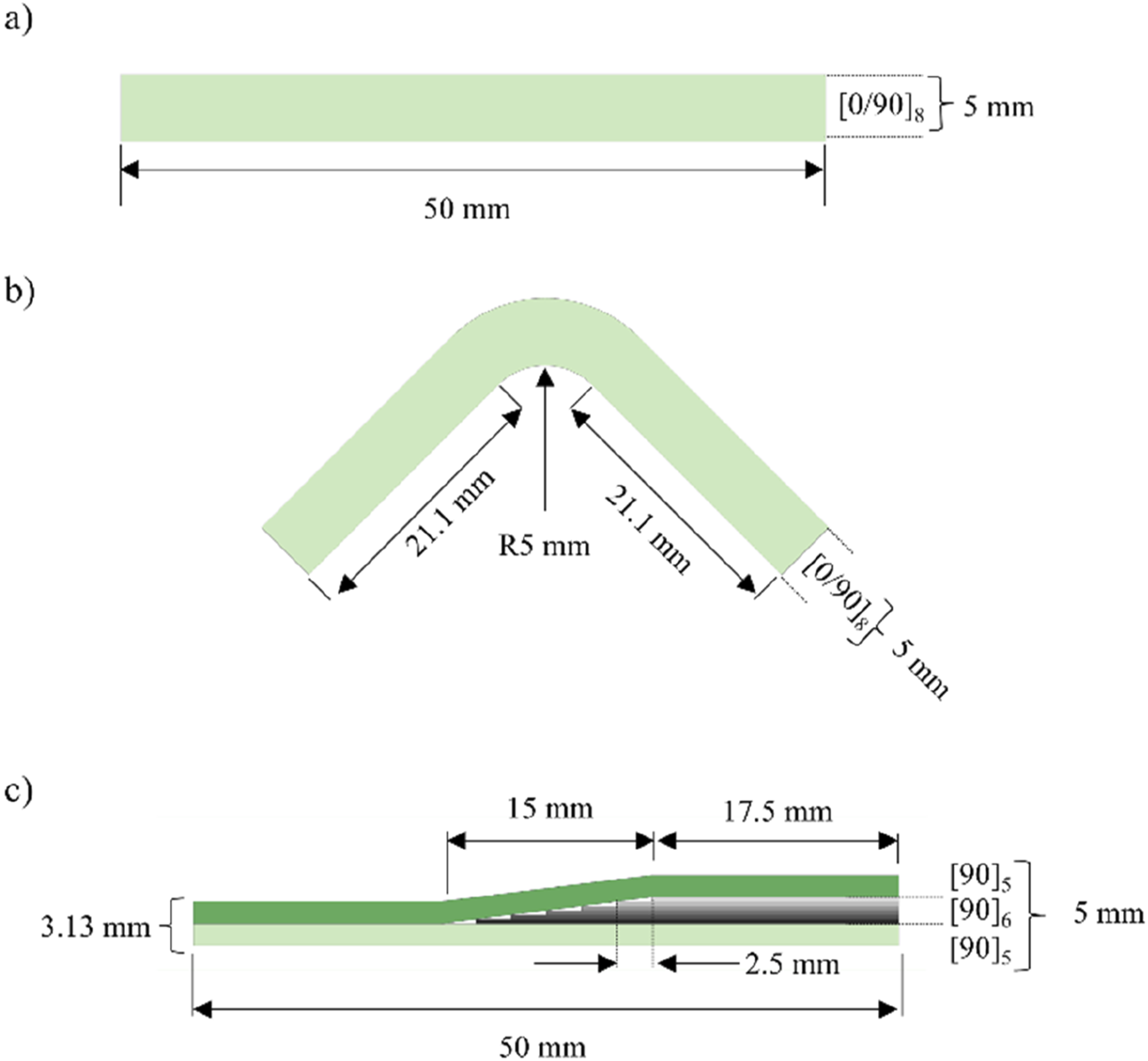

The three samples were manually laid-up before placing them on top of the Nylon tools according to the orientations shown in Figure 2(a) and (b). No intermediate debulking was applied during the lay-up process. A larger aluminium tool, with the same corner radius as the nylon corner tool, was used to facilitate the lay-up of the corner sample. After transferring the samples to the nylon tools, a Vacuum Bag Only (VBO) configuration was implemented using the set of consumables shown in Figure 2(c) and (d). Release films were used to separate the sample from the mould and the breather cloth. An edge breathing dam, consisting of a cork piece wrapped with fibreglass cloth, was placed along the shorter edge of the sample to facilitate air evacuation out of the sample. Finally, the vacuum line was connected and sealed to the vacuum port of the mould prior to installing the vacuum bag. A high quality vacuum level (3 kPa) was achieved throughout the entire manufacturing cycle of the three samples, resulting in a consolidation pressure of 98 kPa.

Figure 2.

CAD design of (a) the corner tool and (b) the flat tool. The sample is displayed in red and the fibre orientation is indicated for each. VBO layup of the flat sample (c) showing the placement of the edge breathing before vacuum bag sealing, and (d) final bagged configuration.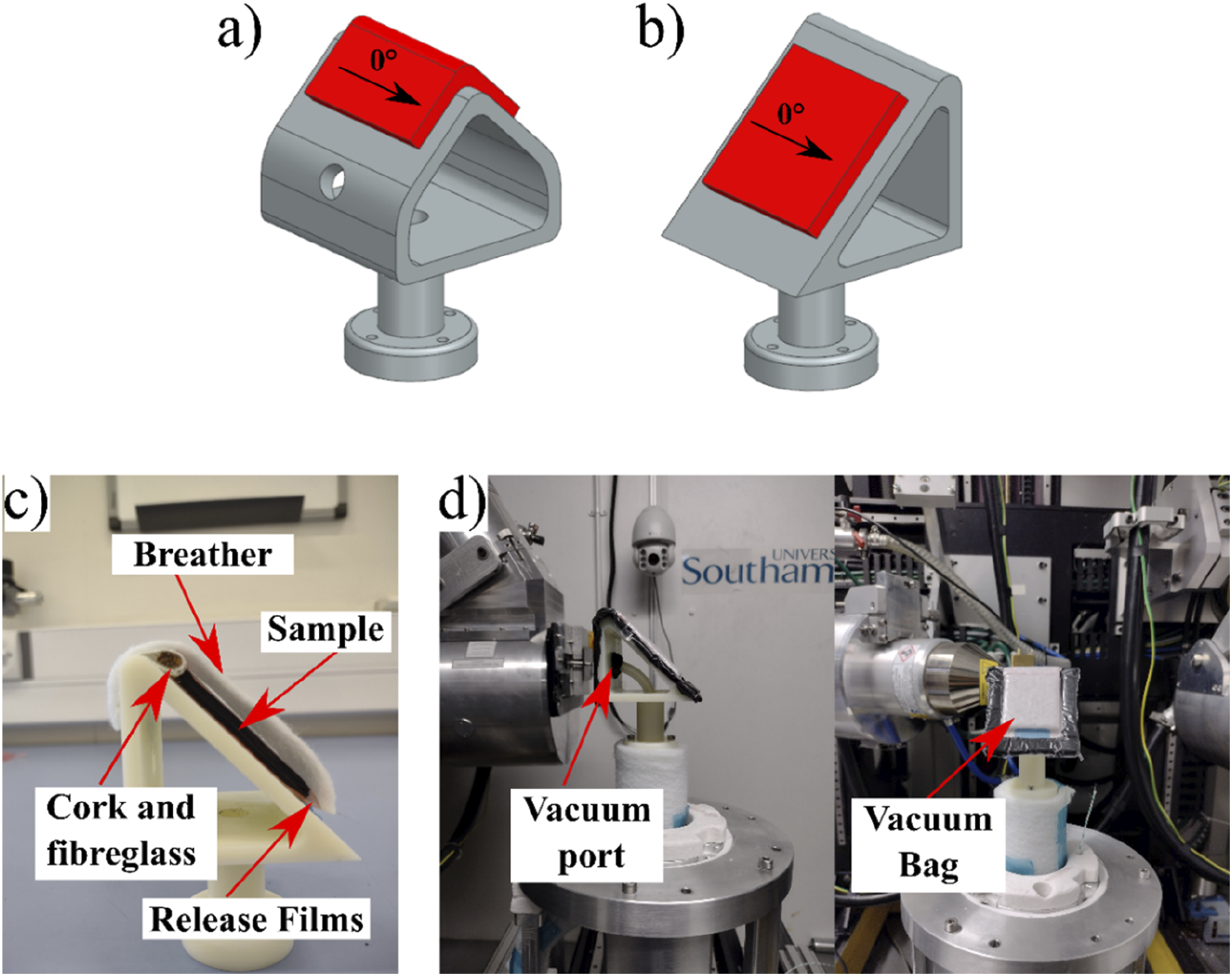

In Situ XCT rig

A custom XCT rig was developed to facilitate the OoA consolidation and cure of composite laminates under In Situ XCT conditions (Figure 3). It consists of two main components. Firstly, a frame was attached to the static stage of the CT-scanner to support the oven cover and the in-line heater (Watlow Fluent with internal baffles). Compressed air passes through the heater and is blown into the oven, heating the composite sample by convection. The oven cover had an internal diameter of 100 mm, a wall thickness of 5 mm, height of 200 mm and was made of the same cast Nylon 6 as the tools. Secondly, the Nylon tool is placed on top of a shaft connected to the rotating stage of the CT-scanner to rotate the sample and collect the 360° images needed for subsequent 3D reconstruction. The vacuum line, providing VBO consolidation of the sample (Figure 3(b)), runs through the centre of the shaft and is connected to a vacuum pump located outside the CT-scanner (Figure 3(c)). Vacuum level was monitored using a vacuum gauge placed in parallel to the vacuum circuit. Two K-type thermocouples were used to control and monitor the temperature within the oven. The thermocouples were placed on top of the oven cover, right above the sample but out of the field of view (FOV) (Figure 3(d)).

Figure 3.

Experimental setup: (a) the oven between the X-Ray source and detector, (b) VBO configuration of the corner sample, (c) CAD design of the rig, and (d) location of the thermocouples.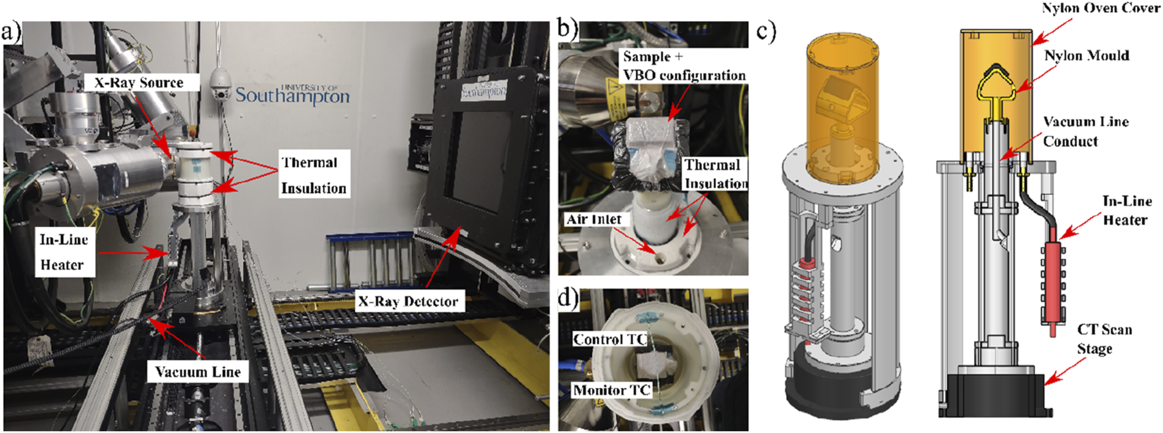

Manufacturing cycle

The three samples were manufactured under OoA conditions. Vacuum was applied for 15 minutes, approximately, before the start of the curing cycle. The material supplier data sheet recommends a curing cycle with a ramp rate between 0.3 and 3°C/min, and a variety of temperatures from 85°C for 16 h to 135°C for 1 h. An initial temperature ramp of 2°C/min was applied in this study until a set-point temperature of 120°C was reached, followed by a 1 h dwell at this temperature. As shown in Figure 4, the part temperature reached 135°C during the curing process. After curing, the oven was cooled to room temperature at a target rate of 10°C/min.

Figure 4.

Cure kinetics and viscosity evolution of the flat sample.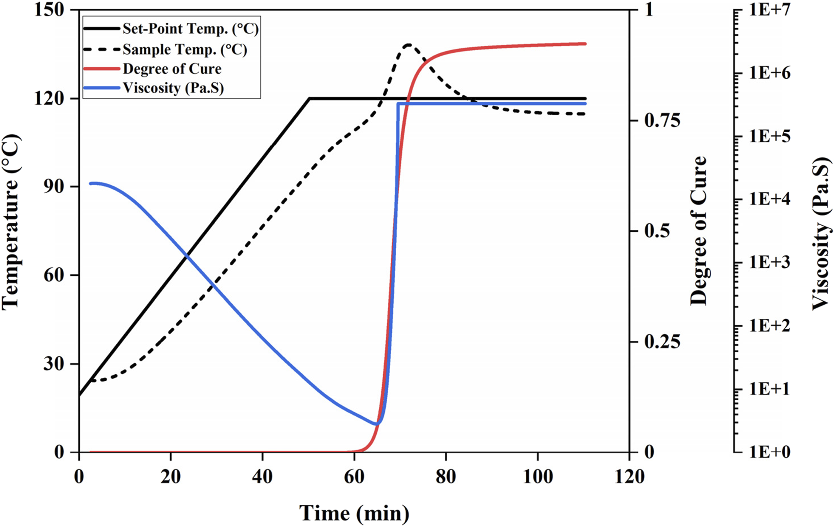

In conventional composite manufacturing processes, a thermocouple is usually placed in the midplane of the laminate edge to measure the temperature history. Introducing a thermocouple in the path of the X-ray would have caused high attenuation and resulted in a bright spot in the area of interest. Therefore, bench trials were performed replicating the heating conditions during the In Situ experiments to correlate the part temperature to the air temperature. Sample rotation that occurs during the In Situ XCT experiment was not replicated during the bench trial and could influence the part temperature.

Previously developed cure kinetics and viscosity models were fit to the measured part temperature from the bench trials to show the thermal behaviour of the epoxy, as illustrated in Figure 4. The cure and viscosity models are provided in Appendix A. The sample and set point temperatures are offset by 2.5 min to account for the difference in the initial temperature of the bench trial (24.5°C) and the In Situ experiments (19.5 ± 1.1°C). The temperature profile of the part reveals an exotherm which initiates after 60 min into the cycle (∼110°C) and increases the part temperature up to 138°C. At this point the viscosity also reaches its minimum and the cross-linking is initiated at around 68 min into the cycle, going from uncured to a degree of cure of 0.9 in just under 20 min. This rapid curing, arising from the exothermic reaction, is evident from the sample temperature rising above the set-point temperature.

In Situ XCT settings

Three in situ XCT experiments, one for each sample, were performed at the µ-VIS Imaging Centre at the University of Southampton with a custom dual-source Nikon 225/450kVp system, using a microfocus 225kVp source with a tungsten reflection target and a Perkin Elmer XRD 1621 CN03 HS flat panel detector. Following the data acquisition, each of the scans was reconstructed by Filter Back Projection (FBP) using the Nikon CT Pro software, resulting in a 32-bit greyscale 3D volume image of 1000 × 1000 × 1000 voxels.

The same set of XCT parameters were used for all the scans performed across the in situ XCT experiments. The source voltage and power were set to 120 kV and 33 W, respectively, and the detector was binned 2 × 2 times, resulting in 1000 × 1000 detector pixels. The source to object and source to detector distances were 82.93 mm and 1325.56 mm, respectively. The above setting resulted in a reconstructed voxel size of 25 µm and a FOV of 25 mm × 25 mm, which was taken from the centre of the sample to avoid capturing edge effects.

The selection of the spatial resolution was based on minimising the distance between the X-Ray source and the oven cover so that partial volume effects was reduced and the visualisation of micro-voids was enhanced. The partial volume effect is the grey scale representation of two or more material phases smaller than the XCT scan voxel size as the average of their X-ray attenuation, which can limit their detectability. ⁴⁹ Further increasing the voxel size would allow the capturing of a larger sample volume but also hinder the correct visualisation and further segmentation of micro-voids and tendency towards overestimation of macro-voids.^50,51

The samples were consolidated and cured while a series of consecutive scans captured the process, which ran uninterrupted. 60 scans were performed to capture the evolution of each sample during manufacturing. The first 47 scans captured the temperature ramp and the temperature dwell, while the remaining 13 scans captured the cooling phase. The total duration of a single In Situ XCT experiment was 2.5 h approximately, including the cooling phase.

A total time of about 2 min/scan was achieved by recording 1701 projections at an exposure time of 67 ms per projection during a 360° rotation. For each scan, an additional 30 seconds was needed to allow the rotating stage to rotate back to the initial position before starting the next scan. The resulting reconstructed 3D images depicts a 2 min averaged state of the scan, representing a 3.5X improvement of previous lab-based In Situ CT scanning of composites manufacturing. ⁴³

Image processing

The reconstructed volumes were analysed in Fiji (ImageJ) ⁵² to quantify the voids within the sample for each scan. All volumes were converted to 8-bit, rotated, and re-sliced so that the 0° plies are orthogonal to the screen. A Gaussian filter (sigma radius of 1) was applied to denoise the data based on previous successful segmentation by Deep Learning X-ray CT scans captured in 2 min and having a voxel size of 25 microns. ⁴⁸ The Gaussian filter is a special case of the mean filter and has been widely used in the pre-processing of X-Ray micrographs in the composite field. ³² Histogram stretching was applied to enhance the visual contrast. An additional 45° rotation was applied to the scans of the flat and tapered laminates to position the mould surface parallel to the x axis (Figure 5(a)). Thermal expansion of the Nylon tool during the experiments induced a vertical movement of the tool and sample, which was corrected to ensure that the assessed volume was the same across all the scans. To maximise the amount of material that was analysed from each sample and considering the physical limitations imposed by the different samples and tool shapes, a final sub-volume of 300 slices of 800 × 800 voxels (7 mm × 20 mm × 20 mm) was extracted from the scans capturing the corner evolution, and a sub-volume of 300 slices of 850 × 800 voxels (7 mm × 21.25 mm × 20 mm) was considered for the samples processed on the flat tool (flat and tapered samples).

Figure 5.

Images from the in situ experiment of the flat sample: (a) XCT image, (b) the phase segmentation provided by entropy thresholding, and (c) phase segmentation by Deep Learning.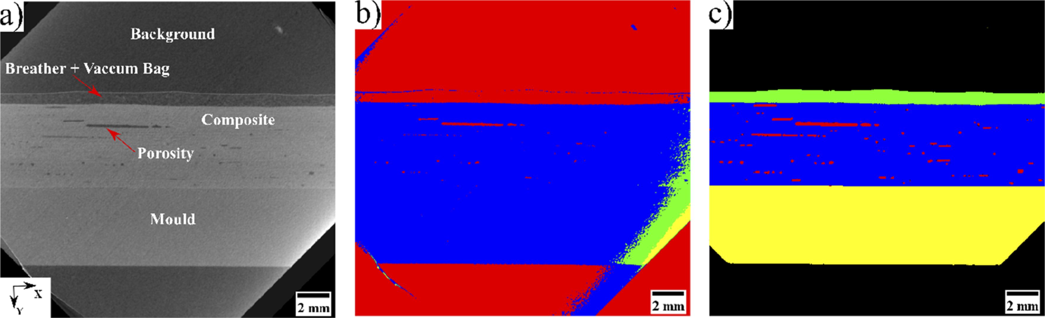

The final step of image processing consisted of the segmentation of the porosity within each sample. This process was particularly challenging as five different phases (background, breather and vacuum bag, composite, mould, and porosity) were present in the reconstructed greyscale images, as shown in Figure 5(a). Even though the background is mainly composed of air, it should be differentiated from the voids within the sample and must be considered as a separate class during segmentation.

A preliminary trial considered the application of the Otsu ⁵³ and entropy ⁵⁴ thresholding algorithms to provide the phase segmentation. To facilitate the threshold determination, the background and porosity phases were considered as a single phase. The phase segmentation provided by the entropy method is shown in Figure 5(b), which was found to provide a better overall segmentation than by the Otsu method. Additional information for and analysis of the thresholding segmentation is provided in Appendix B. The visual results in Figure 5(b) illustrate the poor performance of the thresholding approach to the separation of phases having a comparable density, such as the Nylon mould and the composite sample. This limitation highlights the need for the use of a segmentation technique that is not based uniquely on the greyscale, but also considers other properties, such as texture or pixel context.

Deep learning semantic segmentation using Convolutional Neural Networks (CNN) ⁵⁵ was performed via the definition of an architecture combining convolutional layers with other types of layers (e.g., fully connected, dropout, etc…), and displaying different connections between them. ⁵⁶ The resulting CNN automatically assigns a class to each of the pixels in an image after being trained with an image set formed by a set of raw images and their associated ground truths. The network iteratively learns to segment the phases of interest by minimising the error between the ground truth and its own prediction for each raw image in the training set. A network based on the U-Net architecture ⁵⁷ was defined and implemented in Python 3.6 and Tensorflow 2.5. ⁵⁸ This architecture has been applied to the semantic segmentation of composite X-Ray micrographs ⁵⁹ and was successfully used for the segmentation of different phases in 4D XCT datasets. ⁶⁰

In this study, two deep learning models were created, one for each type of mould, using the training workflow described in. ⁶⁰ The models were applied to the segmentation of the five phases in all the scans within each In Situ XCT experiment using the methodology proposed in. ⁵⁹ Deep Learning provided a substantial improvement in the segmentation of the different phases compared to the simple thresholding approach (Figure 5(b)–(c)). Additionally, it was able to differentiate between phases displaying similar grey scale levels, and segmented voids with reasonable accuracy over a wide range of sizes. Further information regarding the Deep Learning segmentation and training strategy is provided in Appendix C.

Microstructure evolution assessment

The evolution of the porosity, average void size and individual void counts were registered for each In Situ experiment. For each scan, the calculation of the porosity was done using the BoneJ plugin, ⁶¹ available in Fiji (ImageJ), from the segmented images (Figure 5(c)). During image processing it is common to eliminate objects with a size below a certain threshold to remove noise to obtain a cleaner segmented image for analysis. ⁶³ Objects with a minimum size of three voxels (i.e. 75 micron structures) were considered here, in line with previous studies, ⁴⁸ where three voxels were successfully used for an equivalent set of X-Ray parameters. Dragonfly ⁶² was used to generate the 3D renderings of the microstructure.

The thickness change occurring over the course of the in situ experiments was also reported for each laminate. The sample thickness was measured at the centre and at the edges of each sample within the field of view of the central 2D slice for each scan (Figure 6). The thickness of the laminates was automatically calculated by a custom-built script implemented in Python 3.6 that provides the y coordinate of the topmost and bottommost pixels of the composite phase for a given x coordinate. It is important to note that to calculate the thickness variation at the edges of the corner laminate, the scan needed to be rotated 45° so that the laminate is parallel to the cartesian axis.

Figure 6.

Location of the ROI (red boxes) for the (a) corner, (b) flat and (c) tapered sample. The laminate thickness was measured at the position indicated by the yellow lines.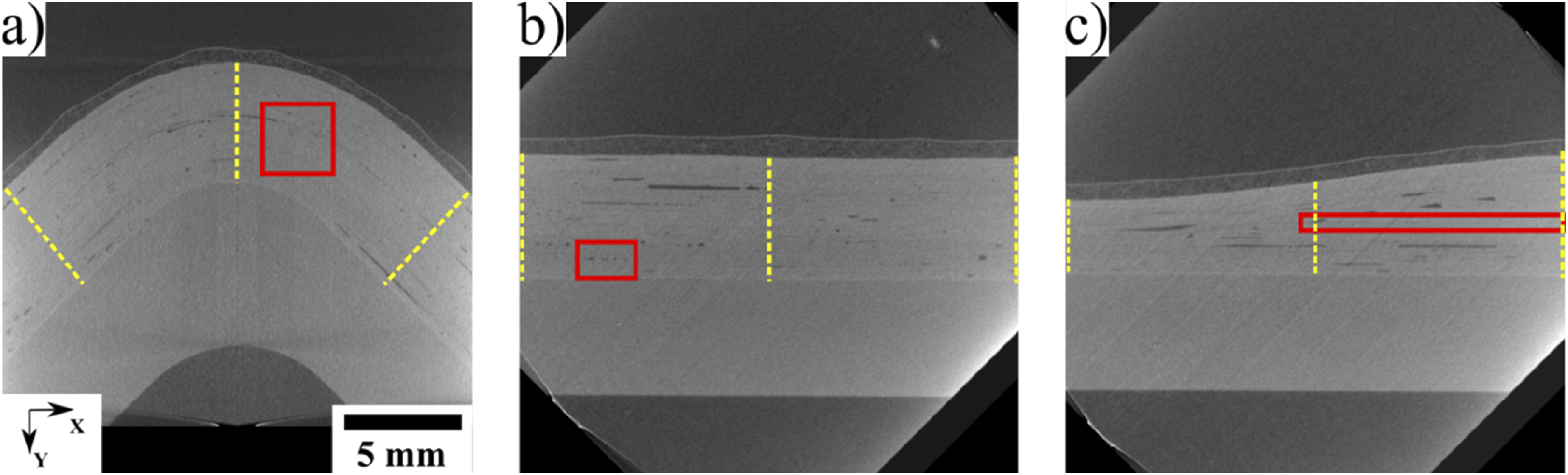

Finally, the void evolution in a sub-region of the original scans were studied by selecting a Region of Interest (ROI) in each sample, as shown in Figure 6. The flat laminate ROI was chosen because it has a porosity level of 2% composed of small volume voids, which is characteristic of the voids in high-performance applications. The ROI within the corner sample captured the changes occurring in the transition zone from the corner apex to one of the laminate arms. Finally, the ROI in the tapered sample covers the evolution of single central ply and its associated ply gap. The location of the ROI was kept fixed throughout the entire set of scans for the given In Situ experiment, and their dimensions were adapted to the morphology of each sample and the feature of interest that was being investigated.

Results

Microstructure evolution

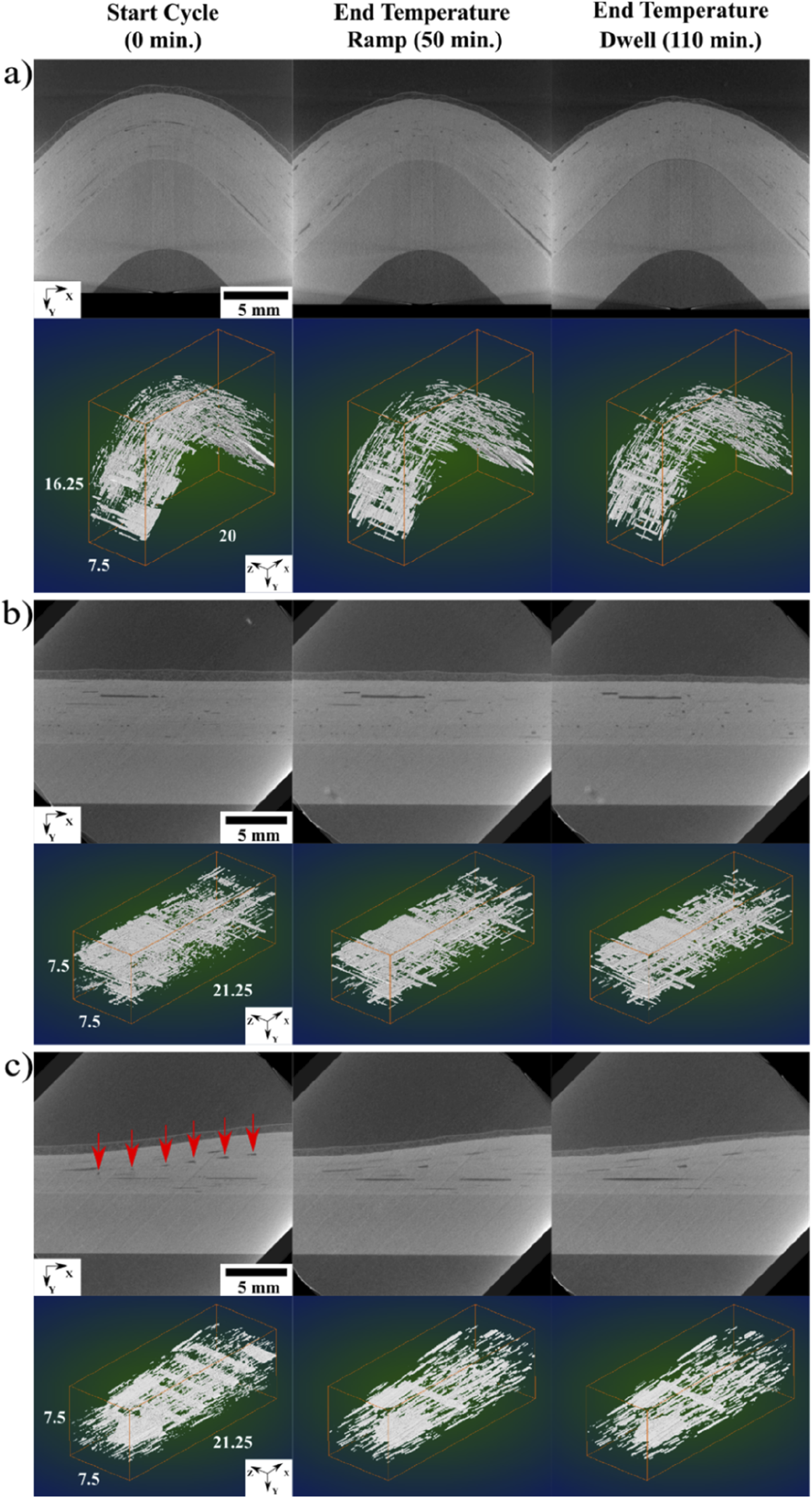
The porosity evolution during consolidation and curing of all three samples is shown in Figure 7. The three samples displayed a similar initial porosity (flat: 3.73%; corner: 3.31% and tapered: 4%), but the porosity evolved differently in each sample during the consolidation and cure process. The first stage of the curing cycle features a temperature ramp from ambient conditions to the 120°C dwell set-point. In this first stage, the resin viscosity decreases according to the profile shown in Figure 4. An increase in the average void volume and decrease in the void counts was observed across the three samples as smaller voids agglomerated. This effect was visually verified in the 3D reconstructions of the three samples and is shown in Figure 8, where the height of the bounding box has been adjusted to exclusively show the volume corresponding to the porosity within the sample.

Figure 7.

Evolution of (a) porosity, (b) average void volume, and (c) individual void counts for each sample during the manufacturing cycle. Resin gelation occurs around 68 min and is marked by the vertical dashed line.

Figure 8.

XCT observations of the (a) corner, (b) flat, and (c) tapered samples at three key points during the manufacturing cycle. The red arrows in the tapered sample point at the location of each of the ply-drops. For each sample, the top row shows the central slice of the scan at the points of interest, whereas the bottom row contains the associated 3D reconstruction of the porosity.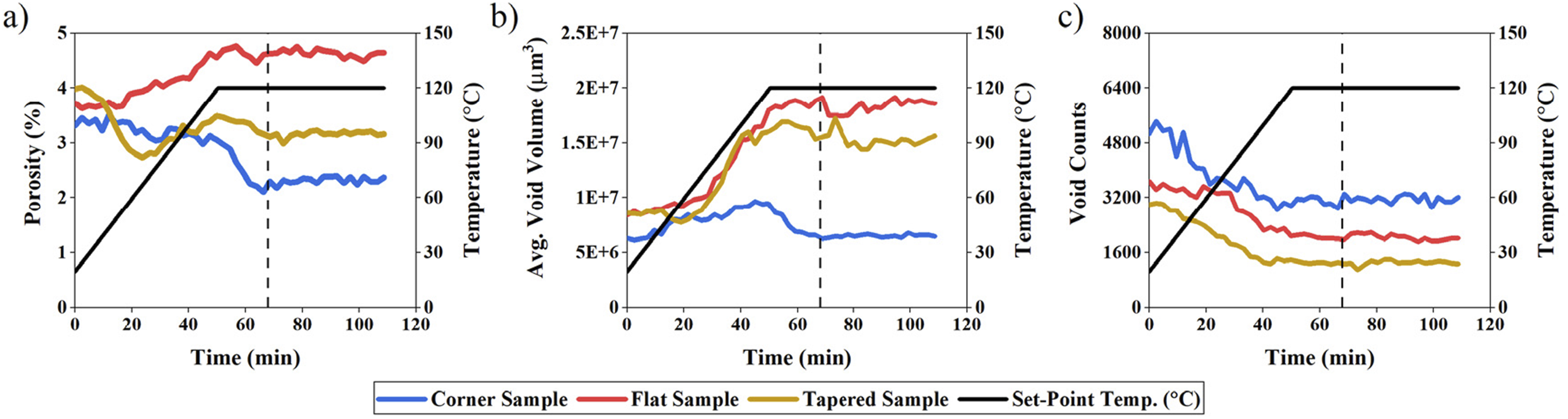

The second stage of the curing cycle covers the constant temperature dwell, where resin gelation occurs, and voids become locked into the microstructure. The third and final stage of the curing cycle was a cool down to ambient conditions. No changes in the sample microstructure were observed at this stage of the curing cycle. For brevity, the results from the cooling stage are omitted.

The porosity in the flat sample increased in the first stage of the cure cycle and reached a maximum value of 4.76% towards the end of the temperature ramp. Porosity remains constant from this point and until the end of the cure cycle. The 3D reconstruction shows a re-arrangement of the porosity distribution as the cycle progresses, consisting of fewer but larger and better-defined voids. The average void volume increases (initial: 8.39 × 10⁶ µm³, final: 18.6 × 10⁶ µm³) and void count decreases (initial: 3685, final: 2013) during the manufacturing process.

The porosity of the corner laminate steadily decreased during the first 50 min, followed by a significant drop during the next 10 min, leading to a minimum value of 2.1%. Resin viscosity is at its global minima during this period. Large voids that initially existed at the edges of the corner sample, and which are noticeable in the 3D reconstruction (Figure 8), are pushed out of the scan FOV once the temperature set point was reached. The removal of the larger voids from the FOV also has a substantial impact on the average void size, which decreased from a value of 9.67 × 10⁶ µm³, reached after 45 min into the cycle, to a value of 6.25 × 10⁶ µm³ in the following 23 min. Removal of the large voids does not substantially change the individual void counts. No relevant changes were observed after gelation, resulting in a final porosity value of 2.4%.

Finally, the tapered sample displays an initial reduction in the porosity value (to 2.73%) after 24 min, as the resin fills the empty gaps created by the ply-drops, which are noticeable in the central slice of the initial scan (Figure 8). The porosity then increased to 3.49% due to voids travelling from outside the field of view into a central ply gap while the resin viscosity was still low. This effect significantly impacts the microstructure evolution for the rest of the cycle and will be analysed in section 3.3.

Thickness evolution

The evolution of the thickness is measured at three locations (right, left and centre of the sample identified in Figure 6) and the results are shown in Figure 9. Gelation is marked in Figure 9 as a vertical line, when in reality it is a window that likely spans 5–10 min. For the material studied here, gelation occurred immediately before the exotherm peak, therefore some thickness change was observed after gelation due to thermal contraction from the exotherm peak of 135°C to the oven set-point of 120°C.

Figure 9.

Thickness evolution registered at three different locations for the (a) corner, (b) flat, and (c) tapered laminates. Resin gelation occurs around 68 min and is marked by the vertical dashed line.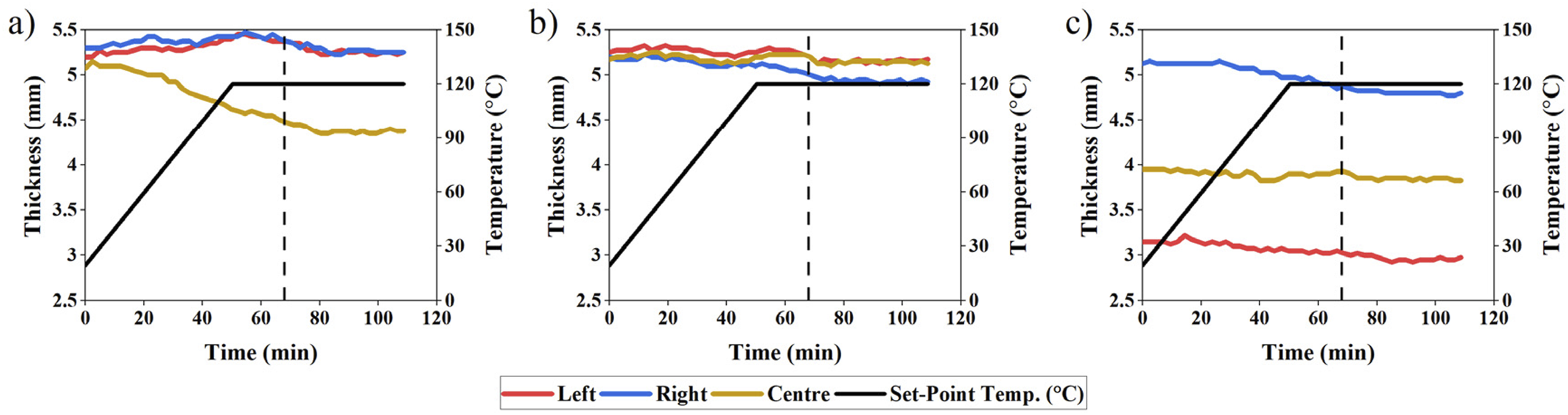

The corner sample initially displays a similar thickness across the three locations, with an average initial thickness of 5.2 ± 0.11 mm. The effect of the external corner consolidation process was a thickness reduction at the apex of the sample, reaching a final value of 4.38 mm (15% decrease). This behaviour contrasts with the evolution observed in the arms of the sample, which exhibit a final thickness of 5.25 mm at both edges, representing a variation of less than 1% from the initial values.

The flat sample has an initial average thickness of 5.2 ± 0.04 mm. The thickness at the rightmost location is reduced by 0.28 mm (6% reduction), compared to a reduction of only 0.08 mm and 0.05 mm (average 1% reduction) in the left and central positions, respectively. This difference can be influenced by the presence of a large void spanning the central and left sub-volume of the laminate and observable in the central slice and 3D reconstructions of the flat sample scan (Figure 8) that hinders the compression of the central and left-hand side of the sample. From these values, the cured ply thickness of a 150 g/m² ply was calculated to be 0.16 mm.

Finally, the initial thickness of the tapered sample is highly dependent on the measurement location due to the central ply drops. The initial measured thickness was 5.13 mm in the thickest region of the laminate and 3.15 mm in the thinnest. The thickness reduction is marginally greater in the thick region compared to the thin region (6.3% reduction vs 5.5%). The magnitude of this reduction is also comparable to the thickness decrease observed in the right edge of the flat sample, where the edge breathing was installed. The thickness measured at the central location reached a final thickness of 3.83 mm (3.1% reduction from an initial thickness of 3.95 mm).

Regions of interest

Three ROI were defined to study the microstructure evolution at specific locations within the samples, as identified by the red boxes in Figure 6. The porosity evolution for each ROI is shown in Figure 10.

Figure 10.

Evolution of (a) porosity, (b) average void volume, and (c) individual void counts within the ROI for each sample. Resin gelation occurs around 68 min and is marked by the vertical dashed line.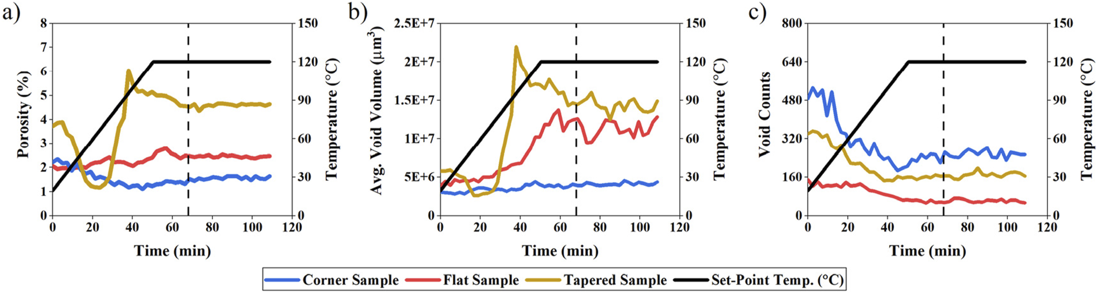

The volume selected within the corner cross-ply laminate (3 mm × 3 mm × 7.5 mm) sees enhanced void mobility in the early stages of the manufacturing cycle. The 3D reconstruction of the porosity evolution is shown in Figure 11. Most of the voids are oriented in the 90° fibre direction at the beginning of the cycle, whereas some isolated voids exist at 0°. This observation is expected because the 90° plies require the fibres to bend over the radius, making ply-to-ply contact more challenging and resulting in a higher proportion of interlaminar porosity. Small objects, identified as voids, are also visible within the entire volume. The initial porosity in this region was 2.22%, and 487 individual voids with an average size of 3.07 × 10⁶ µm³ were reported. After 33 min, the largest void is no longer visible, and the porosity reaches its minimum value (1.1%) after 45 min. At this point in the cure cycle, the lowest number of individual void counts is also reported (186). Porosity slightly increased and reached a final value of 1.63% at the end of the cycle. The average void size remained relatively constant throughout the curing cycle as both larger and smaller voids were re-arranged. The porosity distribution at the end of the cycle is dominated by larger voids oriented in the 90° direction, whereas most of the smaller voids are no longer visible.

Figure 11.

3D reconstruction of the porosity within the ROI defined in the corner sample at different stages of the manufacturing cycle. The largest void is identified by the red arrow and the edge breathing side is identified by the blue line.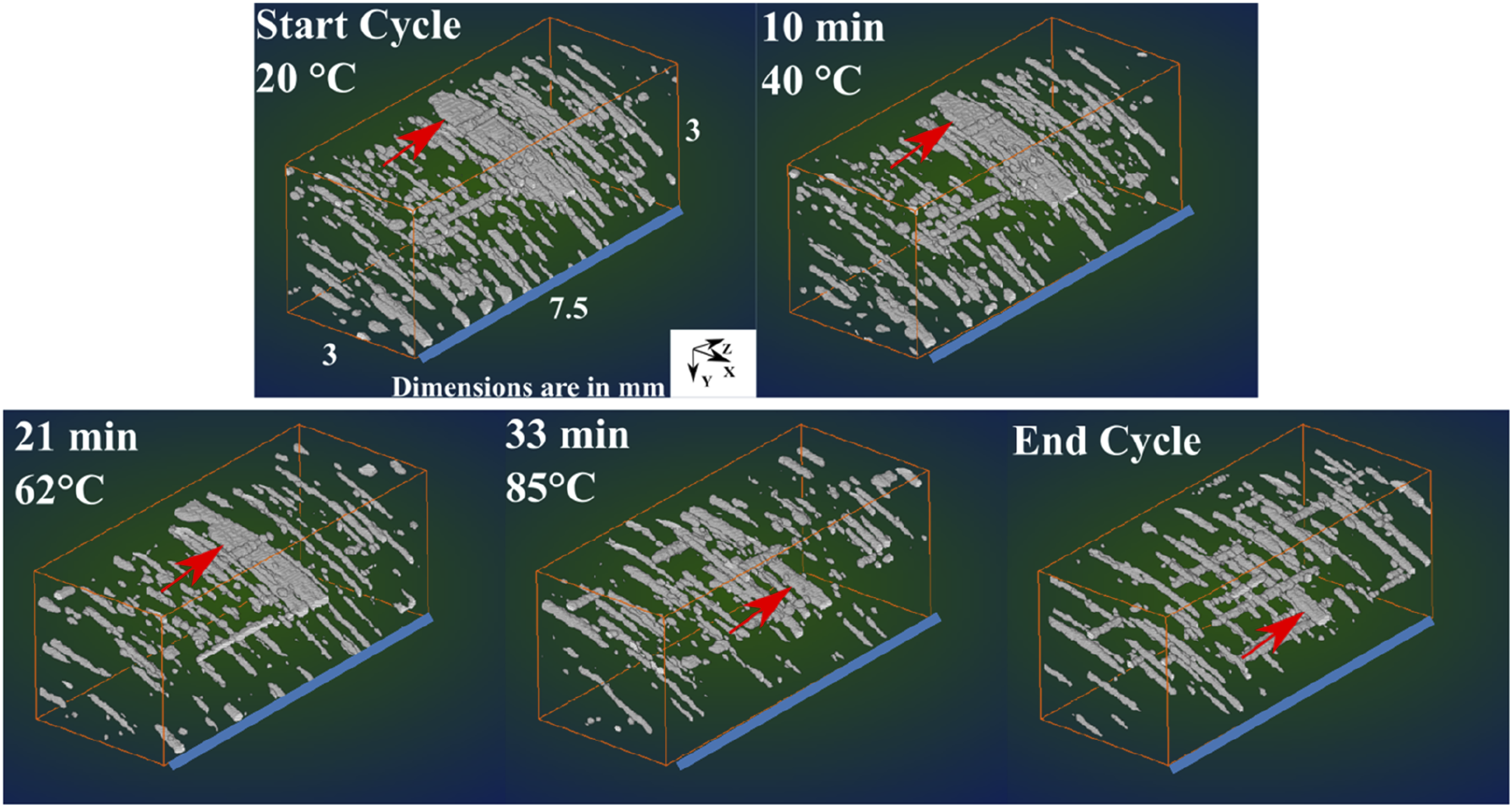

Figure 12 shows the evolution of the porosity within the ROI defined for the flat cross-ply sample (2.5 mm × 1.5 mm × 7.5 mm). This sub-volume is characterised by small and disperse voids, with no predominant orientation at the beginning of the cycle since all plies are laid flat. The initial conditions were a total porosity of 2.05%, 149 individual void counts and an average void size of 3.87 × 10⁶ µm³. As the temperature increases, voids appear to coalesce into bigger voids oriented parallel to the fibre directions. This effect can be visually assessed by the evolution of the void identified by the red arrow and oriented in the 90° direction. The void is initially surrounded by several voids of similar or smaller size and displays an irregular and elongated shape. After 33 min, still in the temperature ramp, the void grows and most of the smaller voids around it have disappeared. At 118°C the void mobility is maximum and the void continues to grow, mainly due to the merging with a large transversal void. By the end of the cycle, the transversal void has completely merged into the 90° void. The porosity at the end of the cycle increased to a value of 2.47%, whereas a substantial increase of the average void size (1.28 × 10⁶ µm³) and a 63% decrease of the void counts (57) was observed.

The 3D reconstruction of the porosity in the tapered ROI evolution is shown in Figure 13. The ROI dimensions are 11.25 mm × 0.62 mm × 7.5 mm. The initial porosity within this sub-volume was 3.72% and was largely dominated by the void associated to the ply-drop. As the temperature increased, the porosity reached a minimum value of 1.17% after 24 min. Four minutes after this point, a large void entered the ROI and travelled in the fibre direction towards the central part of the sample, inducing the re-appearance of the central ply-drop gap. The large void travels in the opposite direction to the location of the edge breathing, creating a sudden increase in porosity within the ROI, which reached a maximum of 6.04 %. A substantial increase of the average void size was also observed. As the large void settled within the central ply-drop gap, the final porosity decreased to a value of 4.63%.

Figure 12.

3D reconstruction of the porosity within the ROI of the flat sample at key stages of the manufacturing cycle. The red arrow points at a large void that enters the ROI field of view and merges with the ply-drop gap. The edge breathing side is identified by the blue line.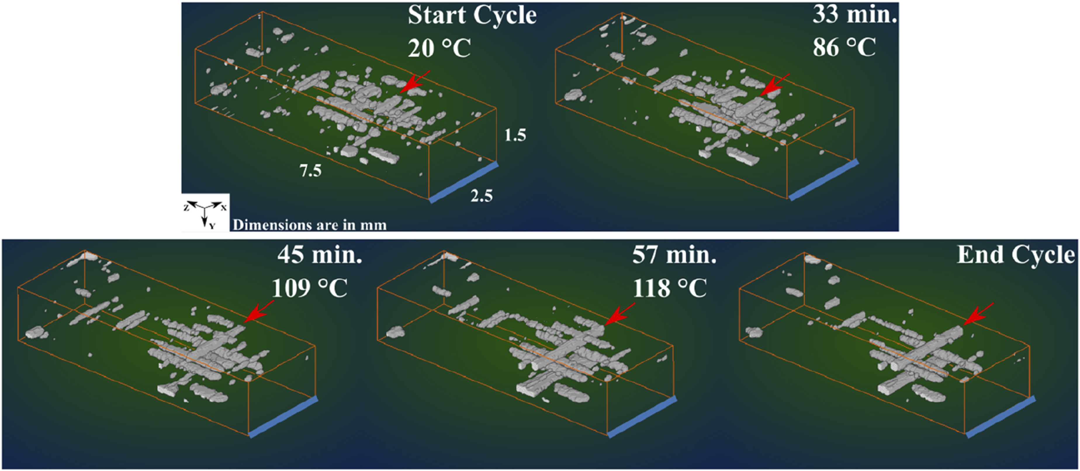

Discussion

The newly developed combination of lab-based In Situ XCT and deep learning segmentation was used to observe and quantify the microstructural changes for prepreg laminates processed using oven VBO curing. This methodology enabled the use of larger volumes, complex shapes and 3.5 times faster scan times compared to the current state-of-the-art. ⁴¹ Even though further repeats and an expanded test matrix are required to account for variations and inhomogeneities found in composite materials, some observations from the current study align with previous work in literature, while others were more surprising.

A common trend in the porosity evolution was observed across all three samples, where voids re-arrange into fewer but bigger volumes that are mostly oriented parallel to the fibre direction. This effect was particularly visible in the volume reconstruction (Figure 8) and in the sub-volume analysed within the flat sample (Figure 12), where the initial void distribution, characterised by small and disperse voids, merged into fewer but larger rod-shape voids as the consolidation process progressed. This final void morphology has been observed in previous work in literature ⁶³ and the current study is able to visualise the formation of these morphologies in real-time.

Figure 13.

3D reconstruction of the porosity within the ROI defined in the tapered sample at different stages of the manufacturing cycle. The evolution of the large void is identified by the red arrow and the edge breathing side is identified by the blue line.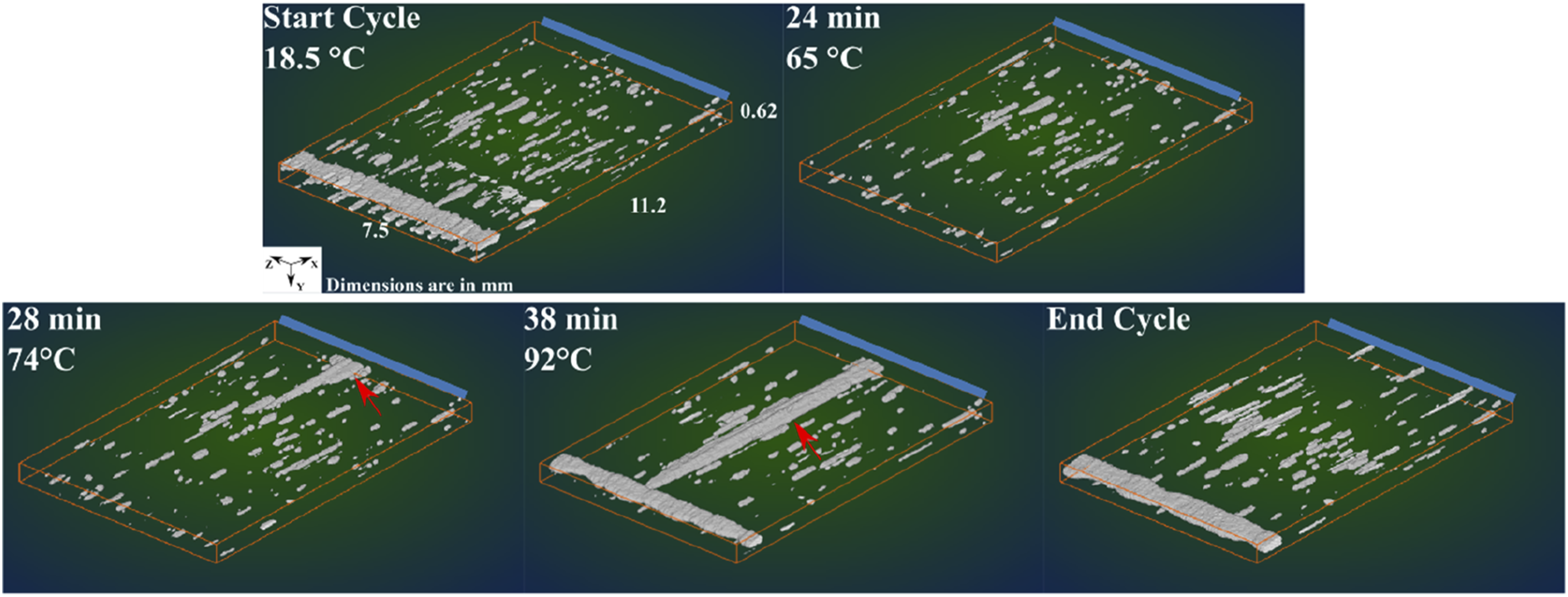

The measured porosity in the flat sample increased by 25% during the manufacturing cycle with an associated increase in void volume but a decrease in void counts. A previous In Situ study on understanding void mechanics used an analogous 2D microscopy configuration by incorporating perforated neat resin film to represent entrapped air. ²¹ In that work, two factors were observed that led to increase in void volume: (1) Pressure equilibrium and (2) Void mobility. The voids expanded if the gas pressure was higher than sum effects of hydrostatic resin pressure and surface tension. As the resin viscosity reduces the resin pressure reduces, which in turn leads void volume increasing. Furthermore, with increasing void mobility voids coalesce thus increasing the volume and void content. The current study enables the visualisation of this temporal phenomenon in a real composite sample.

It is important to note that the final porosity was higher than the initial state in the current study, even though edge breathing was used. This increased void content is potentially due to the exothermic reaction which leaves very little time for key mechanisms to aid in the reduction of entrapped air and expanded voids formed from a variety of reasons, such as moisture. These effects have been previously observed in ex situ studies using OoA prepregs. One study had indicated significant impact on the final void content from thermal gradients and edge breathing arising from closing of evacuation pathways. ⁶⁴ The effect on void evacuation from the closure of pathways can also be observed in the tapered sample in the current study (Figure 8). In these samples, the porosity content closer to the thinner edge is higher than the thicker edge (closest to the edge breather) as it was evacuated earlier in the cycle thus closing the pathways.

The corner samples had a thickness reduction at the apex that was greater than at the arms. This phenomenon of corner thinning of laminates manufactured on external radii have been observed in other studies and is attributed to increased consolidation pressure.^6,7 This increased consolidation pressure on 90° plies in the laminate can lead to percolation or shear flow ¹¹ and will depend on the resin state. In the current form, the In Situ XCT setup is not able to capture these finer flow phenomenon but is able to capture void migration away from the apex of the corner indicating presence of these flow mechanisms at different periods of the process.

Interestingly, the corner laminate separated from the mould tool during the constant temperature dwell, as shown in Figure 14. This separation may be attributed to the development of resin modulus and the ability to carry residual stresses triggered by chemical cure shrinkage and thermal contraction, both of which are known to produce spring-in in composite corner parts. ² Further widening of the gap between the corner part and tool was observed during cool-down due to the mis-match in the coefficient of thermal expansion (CTE) between the fibres and resin. As stated in section 2.1 the corner laminate did have a cross-ply [0,90]₈ lay-up, and while balanced, the lay-up is not symmetric. Lab-based In Situ CT could be used to better understand how and when the distortion develops during the manufacturing process, and compliment the methods available to predict dimensional stability and residual stresses. ²

Figure 14.

The corner laminate at (a) the start of the cycle and (b) the end of the temperature dwell. The top row shows the central slice of the scan with the red arrow pointing at the space between the composite and the mould. The bottom row displays the 3D reconstruction of the porosity (white) and the space between the sample and the mould (orange).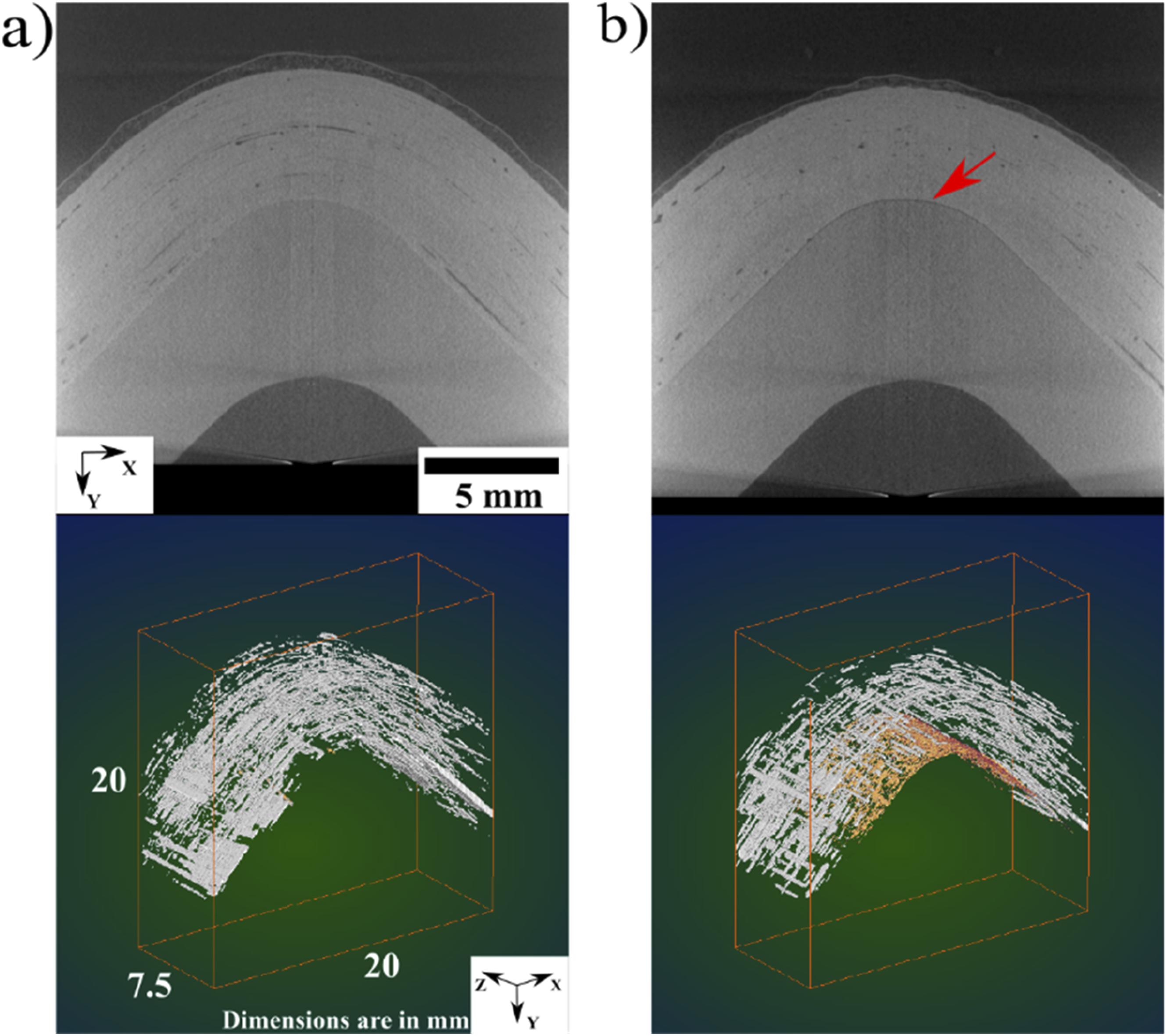

The evolution of the tapered sample showed a first stage where a sharp decrease in the porosity (31% reduction) was observed. However, an unexpected large void was observed re-entering the FOV and progressing in the opposite direction to the edge breathing (Figure 13). There was no drop in vacuum during the process and thus the reason for this observation cannot be fully ascertained.

There are limitations in the current study in terms of the need for more samples to confirm the observations. Furthermore, the void content analysis of the FOV could be affected by the directionality of the void mobility arising from single edge breathing. However, the current study does show the role In Situ XCT can play to relate part complexity, microstructural evolution, processing conditions and material properties.

Conclusions

A new methodology for faster In Situ lab-based XCT was developed for observing time-resolved void interaction and ply consolidation in composite laminates during oven vacuum bag moulding. The rig can run an uninterrupted cure cycle typical for high performance composite with a ramp rate of 2°C/min and peak temperature of 120°C. The custom rig and XCT parameters were optimised to achieve a 2-min scan time at voxel size of 25 µm. The scans were analysed using an improved deep learning image processing technique to study the microstructural evolution in three composite sample geometries: (1) Flat, (2) Tapered and (3) Corner. The rig combined with the deep learning technique allowed for faster scanning of larger and more complex samples compared to previous lab-based in situ XCT studies, reducing costs significantly compared to synchrotron methods.

From the proof-of-concept scans performed in this study, the following observations under the vacuum bag were seen in real-time:

• Void interaction in flat and tapered laminates: small and disperse voids merged into fewer but larger rod-shape voids as the consolidation process progressed.

• Thinning at the apex of external corners relative to the arms: voids migrated away from the apex of the corner but finer details of any resin and/or fibre flow were not captured.

• Laminate separating from the tool during the process: associated with the development of resin modulus and ability to carry stress.

Additional samples need to be tested to verify the reproducibility of the observations outlined above.

In Situ lab-based XCT combined with deep learning segmentation has proved to be a powerful and cost-effective tool to provide high-quality data capturing and time-resolved material behaviour. While shorter scan times could enable further information and time fidelity of the experiment, there are signal to noise limits that cannot be overcome without changing the source and detector hardware. Further investigations may well build on this initial work but the combination of kV, power, exposure time and number of projections was able to provide sufficient image quality for the purposes of observing void interaction and ply consolidation in composite laminates. With additional samples, this technology can be applied to study and optimise cure cycles for a wide range of industrial applications.