Sage Journals: Discover world-class research

Abstract

Fast and accurate methods are required to predict stresses in the vicinity of open and closed holes in composite structures, especially in a global-local modelling context as applied during the design of airframe structures. Fast analytical solutions for infinite-width anisotropic plates with open holes do not consider finite-width effects. Heuristic methods and semi-analytical solutions can be used to towards addressing such effects. To improve the accuracy and speed of these respective methods, we use machine learning (ML) methods trained on high-fidelity finite element analyses to make finite-width corrections. However, such methods require large amounts of training data to reduce errors to satisfactory levels. Therefore, in this study, the fusion of analytical solutions with machine learning is performed. We develop an analytical solution-informed ML model that is as fast as an analytical solution and superior in accuracy to analytical solutions with heuristic finite-width scaling. Our informed ML model offers accuracies equal to analytical solutions for the infinite-width case, and it is capable for use in a global-local modelling context, under uniaxial and biaxial loading. Our informed ML model outperforms prediction accuracy across all cases compared to uninformed ML models and requires a significantly lower size training dataset size.

Graphical Abstract

Keywords

Composites global-local finite-width open holes finite element analysis machine learning

Introduction and literature review

Open holes and closed holes (pinned holes and bolted joints) are common in composite structures,¹ and it is important to accurately predict their failure in a fast and virtual manner to enable sizing and optimisation studies of large composite structures. Progressive damage modelling requires high-fidelity meshing, a failure criterion and a degradation model. Therefore, progressive damage models are computationally expensive. Analytical methods have been developed in order to make faster predictions. Analytical methods to predict failure as a result of stresses at the hole edge result in conservative predictions.^2,3 Therefore, non-local semi-analytical approaches to predict failure have been developed.

The most popular of these approaches is the characteristic length method. This method is based on evaluating the failure indices using stresses at/over a given distance from the hole boundary.⁴ This distance lies perpendicular to loading, in the net section plane, for open hole composites, and it may also exist parallel to loading, in the bearing plane, for bolted joint analysis.⁵ In this method, stress analysis can be conducted using linear-elastic finite element analysis and therefore substantial computational expense is saved. Analytical methods for open hole stress analysis, such as those based on Lekhnitskii’s formalism,⁶ reduce computation expense further. Modifications built on this formalism are used in the bolted joint stress field model which is popular in industry,⁷ and combined with composite laminate theory, to apply the characteristic length method to bolted composite joints.

The Lekhnitskii formalism assumes an infinite plate.⁶ However, in application, free edges due to structure boundaries or due to nearby holes affect stress distribution and so finite-width effects require consideration. Various methods have been developed to generate finite-width correction factors. Heuristic methods scale stresses to conserve section forces,^8,9 but lack accuracy in capturing the change in stress distribution due to finite width. Semi-analytical methods based on auxiliary functions or boundary collocation can be used to satisfy finite-width boundary conditions,^10,11 however, their computational time and prediction accuracy varies with the amount of series truncation and boundary collocation points. Finite-width correction factors can also be derived by correction of failure strength and require a failure prediction model¹²; however, errors in this failure prediction model are not fully considered in Ref. 12.

In this work, we aim to use machine learning to modify predictions based on Lekhnitskii’s formalism, to account for finite-width effects. Machine learning methods use fast matrix multiplication and can deal with problems with non-linearities particularly well. This makes them suitable for an attractive compromise between speed and accuracy in comparison to existing methods.

Machine learning can be used to predict stress fields directly with numerical training data as in previous studies for composites structures. In such studies, image-based neural networks such as convolutional neural networks, U-nets, and generative adversarial networks are used to predict stress fields.^13–15 In a previous study, we used sequential neural networks to predict through-thickness stress distributions in a global-local multifidelity context.¹⁶ The study involved the development of an improved design of experiment, input and output feature engineering and neural network customisations to enable the machine learning methodology.

However, the numerical finite element methods used to generate training data can still be time-consuming. Furthermore, the physics information in these machine learning models is limited to numerical data. In this study, we propose the addition of physics information via analytical methods. The machine learning model aims to correct the approximate solution given by the analytical solution. The use of computationally efficient analytical solutions to inform the input of these machine learning models may result in higher accuracy predictions and/or reduce the amount of numerical data required to train the machine learning models.

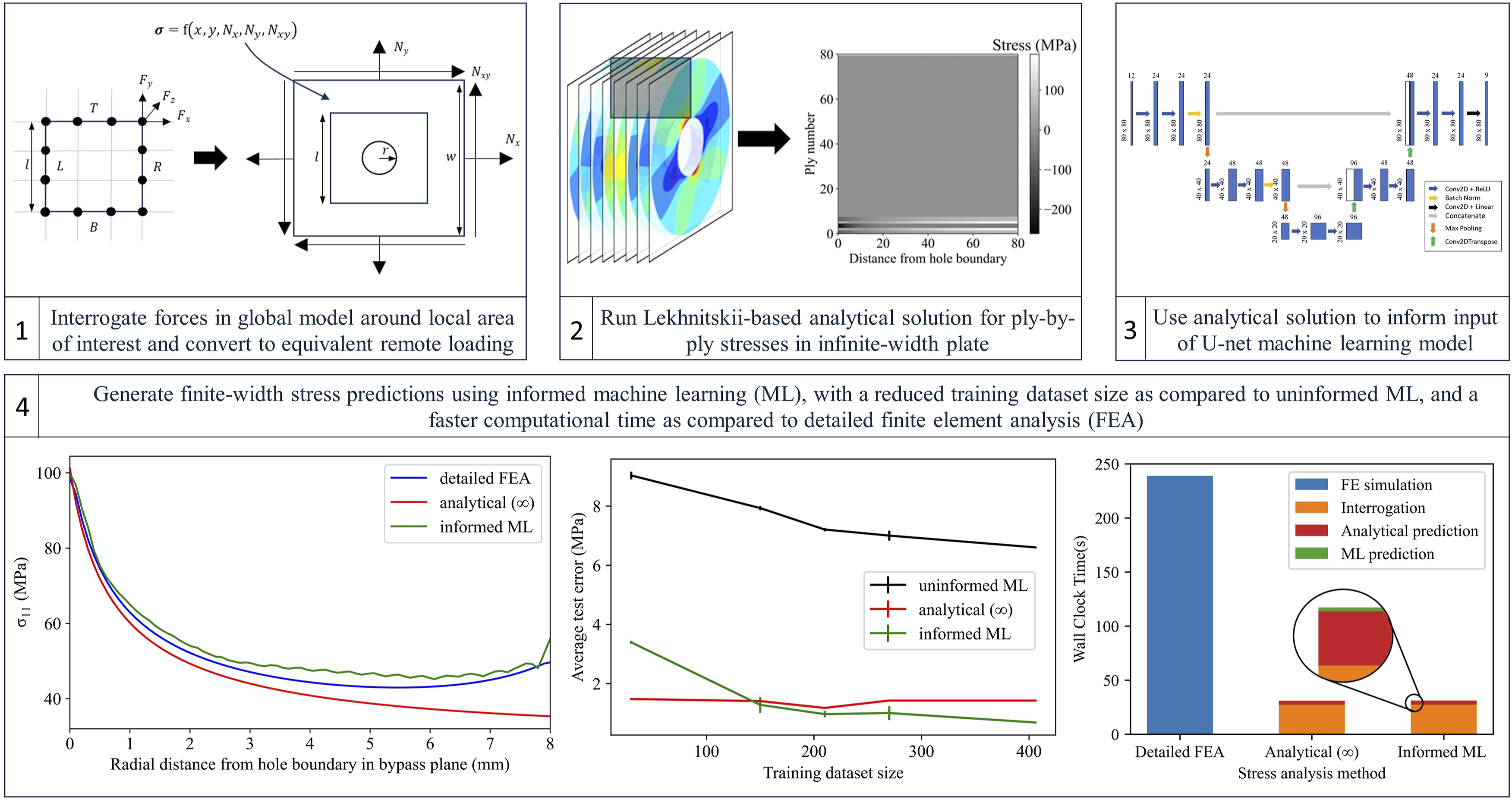
In order to embed the analytical solution-informed machine learning model into the global-local submodelling procedure, we also develop a method to interrogate the forces from a global model which may not have a fully represented hole feature. These forces are to be converted into remotely applied unit loads for input to the physics-informed machine learning model. This is performed under uniaxial and biaxial loading conditions.

In this study, we focus on open hole stress analysis and therefore the stresses in the net section plane. Overall, we show that the analytical solutions used in this study are both improved by the machine learning model and used to improve the machine learning model for use in multifidelity global-local submodelling frameworks.

Aims and objectives

The objectives of this study are to:

1. Predict the stress distribution around an open hole in infinite-width anisotropic plates with membrane loading using an analytical solution-informed machine learning model.

2. Generate finite-width stress corrections with the above machine learning model.

3. Develop a method to determine the equivalent remote loading applied to the open hole by the global model.

4. Use the machine learning model in a global-local modelling context to predict stress distributions around an open hole.

Methodology

Workflow

The workflow of the code to train and use our machine learning model starts with the generation of samples using a design of experiments method. Open hole laminates of varying hole geometry, $\frac{W}{D}$ ratios and laminate stacking sequences are created. This design of experiment, as according to a previous study,¹⁶ results in well distributed sampling of laminate stacking sequence in both the lamination parameters space and the ply angle space.

Thereafter, analytical solutions and numerical solutions for loading the laminate under varying membrane loads are created and saved. For our analytical solution, we extend the code developed by an online resource,¹⁷ to calculate ply-by-ply stress distributions in the net section plane with Lekhnitskii’s formalism. Numerical solutions generate stresses at nodes, and therefore need to be smoothly resampled using Paraview.¹⁸ These stresses are saved as image files.

The analytical solutions and the design of experiment variables can be used as input features when developing our machine learning model. The output features are the stress field images generated by numerical methods.

In order to use our developed machine learning model, we develop a script that converts nodal forces in a given global model to the equivalent remote loads. Analytical solutions of a given open hole laminate can then be determined, the results of which are improved by the use of our machine learning model to account for finite-width effect. Predicted stresses can then be saved for use as appropriate, with a failure criterion for example to predict failure.

Analytical solution

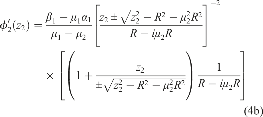
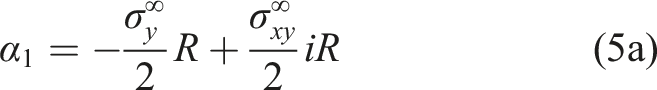
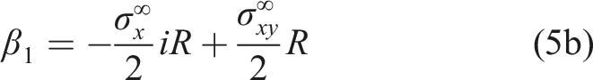
The Lekhnitskii formalism,⁶ which underpins the open hole stress calculation, extends the theory of elasticity to anisotropic materials using complex analysis. The full derivation of the analytical solution⁶ utilises an Airy stress function to satisfy stress equilibrium and compatibility equations in combination with Hooke’s law. In this study, we present the explicit expressions required to calculate stress components. Note that ply-by-ply stresses are calculated using composite laminate theory.

The stress distribution for a single cutout given loading at an infinite width is given by

σ_{x} = 2 R e [μ_{1}^{2} ϕ_{1}^{'} (z_{1}) + μ_{2}^{2} ϕ_{2}^{'} (z_{2})]

(1a)

σ_{y} = 2 R e [ϕ_{1}^{'} (z_{1}) + ϕ_{2}^{'} (z_{2})]

(1b)

τ_{x y} = - 2 R e [μ_{1} ϕ_{1}^{'} (z_{1}) + μ_{2} ϕ_{2}^{'} (z_{2})]

(1c)

where the

x, y

domain is transformed into the complex plane using

z_{k} = x + μ_{k} y f o r k \in {1, 2}

(2)

The characteristic equation below is solved to find the principal roots $μ_{1}$ and $μ_{2}$

a_{11} μ^{4} - {2 a}_{16} μ^{3} + (2 a_{12} + a_{66}) μ^{2} - 2 a_{26} μ + a_{22} = 0

(3)

The first order complex potential function derivates are given by

ϕ_{1}^{'} (z_{1}) = \frac{β_{1} - μ_{2} α_{1}}{μ_{1} - μ_{2}} {[\frac{z_{1} \pm \sqrt{z_{1}^{2} - R^{2} - μ_{1}^{2} R^{2}}}{R - i μ_{1} R}]}^{- 2} [(1 + \frac{z_{1}}{\pm \sqrt{z_{1}^{2} - R^{2} - μ_{1}^{2} R^{2}}}) \frac{1}{R - i μ_{1} R}]

(4a)

ϕ_{2}^{'} (z_{2}) = \frac{β_{1} - μ_{1} α_{1}}{μ_{1} - μ_{2}} {[\frac{z_{2} \pm \sqrt{z_{2}^{2} - R^{2} - μ_{2}^{2} R^{2}}}{R - i μ_{2} R}]}^{- 2} [(1 + \frac{z_{2}}{\pm \sqrt{z_{2}^{2} - R^{2} - μ_{2}^{2} R^{2}}}) \frac{1}{R - i μ_{2} R}]

(4b)

where

α_{1}

and

β_{1}

are given as a function of the remotely applied stresses

σ_{x}^{\infty}, σ_{y}^{\infty}, σ_{x y}^{\infty}

α_{1} = - \frac{σ_{y}^{\infty}}{2} R + \frac{σ_{x y}^{\infty}}{2} i R

(5a)

β_{1} = - \frac{σ_{x}^{\infty}}{2} i R + \frac{σ_{x y}^{\infty}}{2} R

(5b)

Finite element solution

We use Abaqus/2021 to generate our finite element models and run the linear-elastic implicit simulations.¹⁹ Square laminates with a central open hole are modelled. The hole radius is varied from 1 mm to 4 mm, and laminate thickness is varied from 1 mm to 10 mm in the design of experiment. As our plies are of 0.125 mm thickness, this corresponds to varying the number of plies between 8 and 80 plies. The $\frac{W}{D}$ (finite-width factor) ratio is varied between 3, 7 and 10. A ratio of 3 represents minimum finite-width as defined by hole and edge spacing design guidelines.²⁰ A ratio of 10 is used to represent plates of infinite-width, as boundary effects are shown to have dissipated by this distance.¹⁰ In total, 452 training samples were generated.

We use IM7/8852 carbon fibre material with properties as defined in Table 1. Conventional shell elements (S4R) are used, and a convergence study is performed in order to choose the appropriate mesh size. In Figure 1, we compare the stress at the hole boundary in the net section plane as predicted by the analytical simulation and the numerical simulation, of a given laminate [45/-45/0/90]_s with a 4 mm hole and a

\frac{W}{D}

ratio of 10 that is loaded in the x-direction by a given loading (100 N/mm). It is clear that the analytical solution and numerical solution converge using a very fine mesh size of 0.1 mm, therefore this mesh size is chosen for the rest of the study. The selection of a lower mesh density would result in lower-quality training data, and consequently a reduction in the maximum accuracy of the ML model. For example, a mesh size of 0.5 mm would result in a lower bound ML prediction error of ∼63 MPa in the 11-direction, as opposed to ∼0.5 MPa error using a 0.1 mm mesh size.

Table 1.

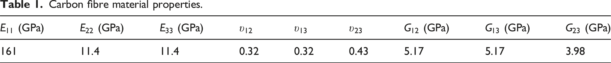
Carbon fibre material properties.

$E_{11}$ (GPa)	$E_{22}$ (GPa)	$E_{33}$ (GPa)	$υ_{12}$	$υ_{13}$	$υ_{23}$	$G_{12}$ (GPa)	$G_{13}$ (GPa)	$G_{23}$ (GPa)
161	11.4	11.4	0.32	0.32	0.43	5.17	5.17	3.98

Figure 1.

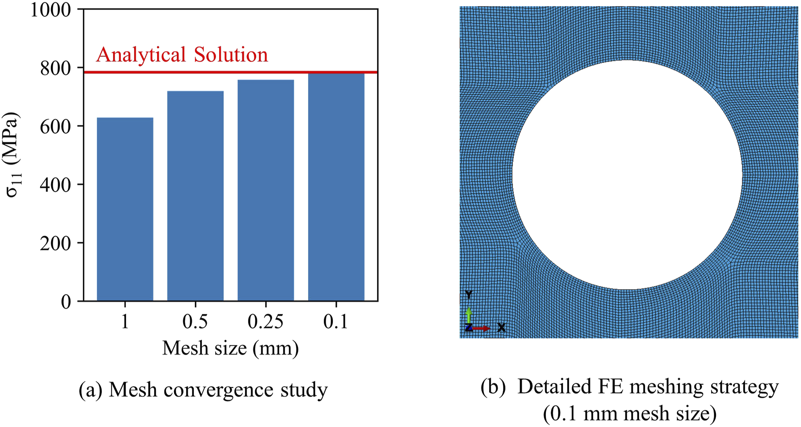
FE modelling details. (a) Mesh convergence study (b) Detailed FE meshing strategy (0.1 mm mesh size). FE: finite element.

Neural network

We use Tensorflow²¹ and Keras²² to develop our machine learning models. Two forms of network are required in this study and are depicted in Figure 2. The uninformed neural network predicts the high-fidelity FE stress field in the net section plane given simple scalar inputs as defined by the design of experiment. The physics-informed neural network additionally incorporates the analytically derived stress fields as input features. To accommodate the different dimensions of input and output between these two networks, the neural network architecture is varied. However, details such as the cost function and optimiser are the same.

Figure 2.

Block diagrams of the neural networks used in this study. (a) Uninformed neural network architecture (b) informed neural network architecture.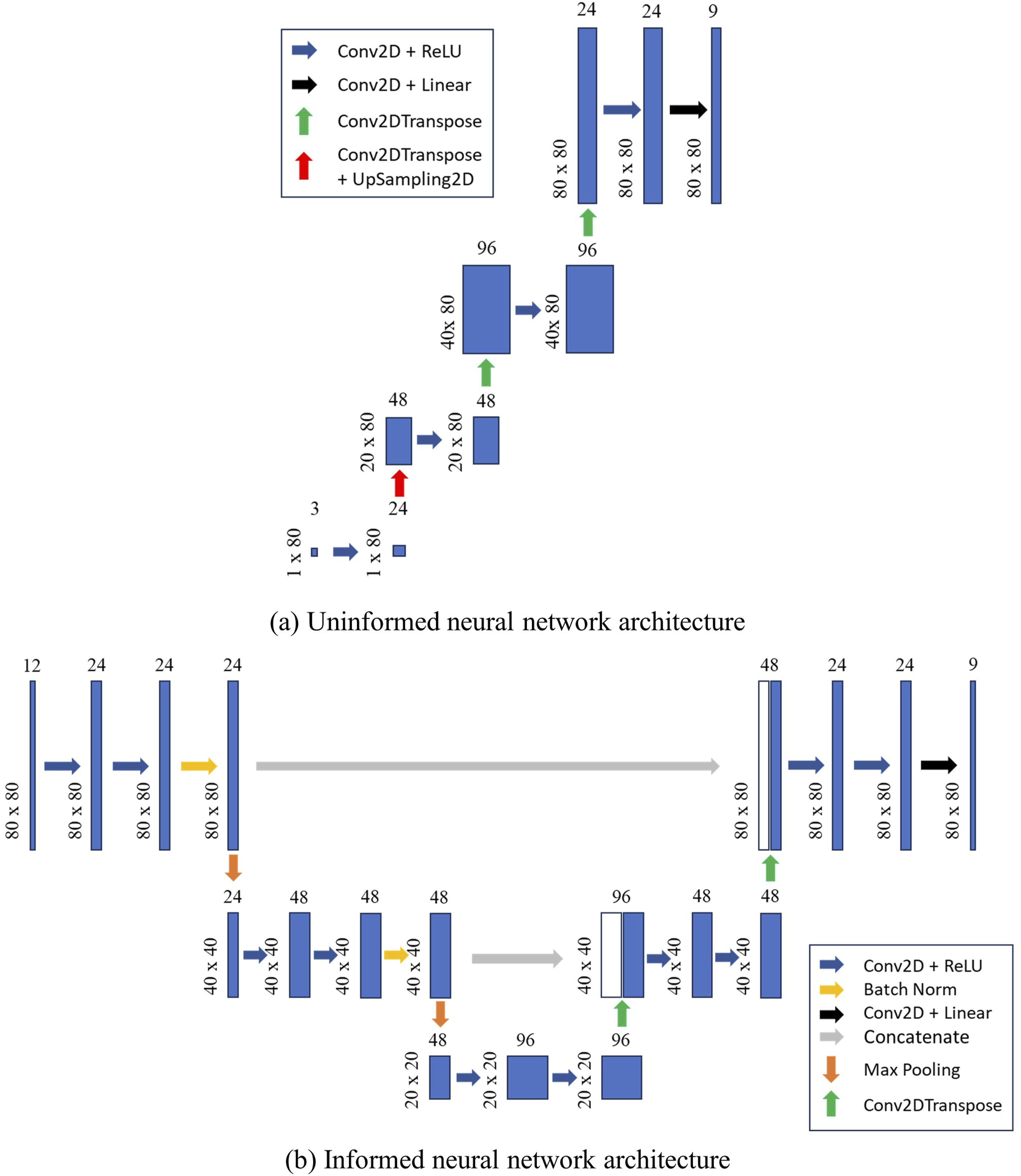

For the uninformed neural network, a singular value for the ply angle, hole radius and finite width factor is given to each of a maximum of 80 plies. Therefore, the input shape is 1 × 80 × 3. Note that for laminates with less than 80 plies, zero values are applied to the respective rows and columns. The output shape is an 80 × 80 stress field for the net section plane, for every 2D stress component given 2D loadings, as generated by FE simulations. Therefore, the output shape is 80 × 80 × 9. This uninformed neural network therefore requires upscaling of dimensions, which is performed using the decoder structure of the convolutional U-net model.²³

The input shape for the second network is an 80 × 80 stress field for the net section plane, for every 2D stress component given 2D loadings, as generated by analytical simulations. This results in an 80 × 80 × 9 matrix, which we concatenate to the 1 × 80 × 3 matrix as described for the uninformed network, to result in an 80 × 80 × 12 input shape. Note that we repeat the 1 × 80 × 3 matrix to make the concatenation compatible. The output matrix is the same as for the uninformed neural network. The inputs and outputs in this second network are therefore of similar dimensions. For this physics-informed neural network, we use the full encoder-decoder structure of the U-net model.²³

We use three-fold cross-validation on a train-validation-test dataset split. We vary the proportions of data in each sub-dataset, to investigate the effect of training dataset size on our model. We use an Adam optimiser, our cost function is the mean absolute error, and we use early stopping to terminate models when this error has converged.

Interrogation of force from the global model

The analytical solution determines the stress field around an open hole within an infinite-width composite plate. However, during the design and predictive virtual testing stage of large composite structures, stresses are interrogated within a global model which is of finite dimensions. We therefore develop a method to interrogate the forces around the local area of interest in the global model, and convert this into equivalent loads applied to a plate of infinite length, see Figure 3. For this, we define a circle of radius $r$ , within a local area of interest of square of side length $l$ and ply thickness $t$ , located in a global model with infinite length and finite width $w$ . Our method is used to interrogate the forces $F$ on the left $L$ , right $R$ , top $T$ and bottom $B$ boundaries of the local area of interest and convert this into equivalent unit loads $N$ applied to a plate of infinite length.

Figure 3.

Interrogation of forces from global mesh and conversion into equilibrated unit forces for input to the analytical model.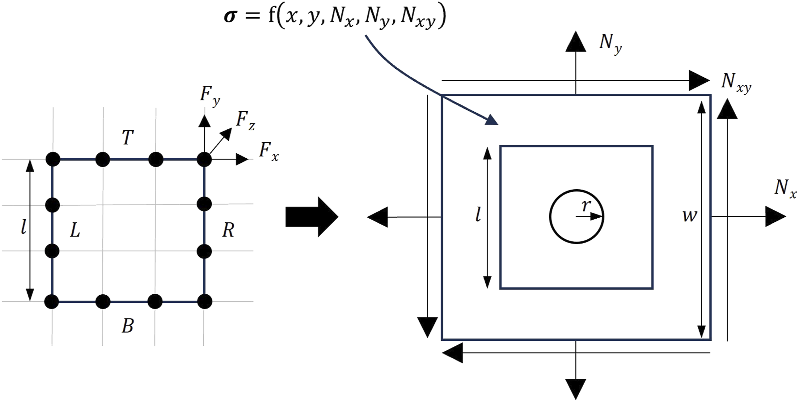

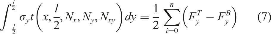
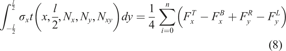
This conversion is performed by appropriately equating the forces at the boundary nodes 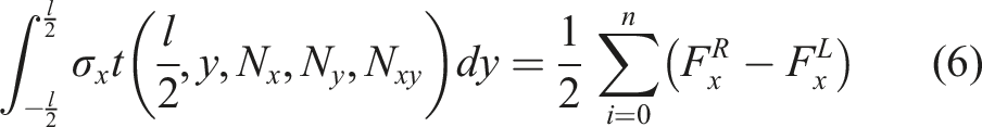$n$ of the local area with the integral of analytically derived stresses at this same boundary. This sets up three non-linear equations

\int_{- \frac{l}{2}}^{\frac{l}{2}} σ_{x} t (\frac{l}{2}, y, N_{x}, N_{y}, N_{x y}) d y = \frac{1}{2} \sum_{i = 0}^{n} (F_{x}^{R} - F_{x}^{L})

(6)

\int_{- \frac{l}{2}}^{\frac{l}{2}} σ_{y} t (x, \frac{l}{2}, N_{x}, N_{y}, N_{x y}) d y = \frac{1}{2} \sum_{i = 0}^{n} (F_{y}^{T} - F_{y}^{B})

(7)

\int_{- \frac{l}{2}}^{\frac{l}{2}} σ_{x} t (x, \frac{l}{2}, N_{x}, N_{y}, N_{x y}) d y = \frac{1}{4} \sum_{i = 0}^{n} (F_{x}^{T} - F_{x}^{B} + F_{y}^{R} - F_{y}^{L})

(8)

The roots of these equations are solved by a modified version of Powell’s hybrid method (a form of gradient descent), which is available within the fsolve function of the python based SciPy library.²⁴

Under the aforementioned root-finding method, our predicted far-field loadings may differ from the actual far field loadings under finite-width. This would then result in the analytical solution used to inform our method being inaccurate, and as a result, the overall ML-enhanced solution may be inaccurate. To correct for this, we can use the reasoning behind the heuristic approach by Tan to finite-width corrections.⁸ The Tan approach correctly aims to ensure that the integral of stresses 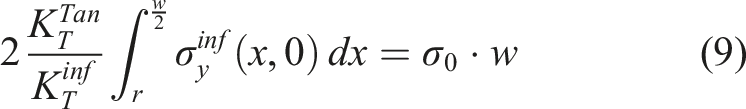$σ_{y}^{\inf}$ across a finite-width is equivalent to the far field loading due to remote stress $σ_{0}$

2 \frac{K_{T}^{Tan}}{K_{T}^{\inf}} \int_{r}^{\frac{w}{2}} σ_{y}^{\inf} (x, 0) d x = σ_{0} \cdot w

(9)

However, for finite-width problems, the Tan factor 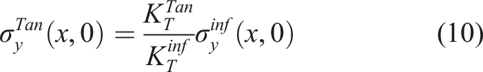$\frac{K_{T}^{Tan}}{K_{T}^{\inf}}$ derived to ensure this equivalence, is uniformly applied to scale the infinite-width solution

σ_{y}^{Tan} (x, 0) = \frac{K_{T}^{Tan}}{K_{T}^{\inf}} σ_{y}^{\inf} (x, 0)

(10)

This therefore assumes that stress decay is equivalent in finite-width and infinite-width settings, and so it is limited in accuracy.¹⁰ However, in our work, we do not propose to use the Tan factor to accurately predict the finite-width stress distribution at the net-section through the hole centre, as that is the role of our ML-assisted model. Instead, we aim to use a modified Tan factor 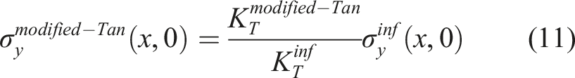$\frac{K_{T}^{m o d i f i e d - Tan}}{K_{T}^{\inf}}$ to scale the integral of stresses at this net-section back towards the infinite-width solution with corrected remote loading (that is unaffected by finite-width effects in the global model) so that we can use this infinite-width solution to better inform our ML-assisted model

σ_{y}^{m o d i f i e d - Tan} (x, 0) = \frac{K_{T}^{m o d i f i e d - Tan}}{K_{T}^{\inf}} σ_{y}^{\inf} (x, 0)

(11)

Our modified Tan correction factor is therefore derived by equilibrating the stresses, not at the net-section width, but on the finite-width cross-section (as determined from the global model) along the boundary of the local area of interest in the infinite-width solution to the remote finite-width loading, using the unit loads predicted from the root-finding methodology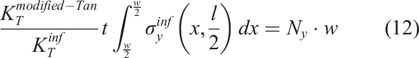

\frac{K_{T}^{m o d i f i e d - Tan}}{K_{T}^{\inf}} t \int_{\frac{w}{2}}^{\frac{w}{2}} σ_{y}^{\inf} (x, \frac{l}{2}) d x = N_{y} \cdot w

(12)

As our models are linear elastic, we can employ linear superposition. Therefore, we can scale machine learning predictions given a unit load, now that we know the total load applied. According to Saint Venant’s principle, the stresses due to statically equivalent loads are approximately the same, at a sufficient distance from the loaded area.²⁵ Therefore, for highly non-uniform global loading conditions applied close to the hole boundary, the accuracy of our method may decrease. However, this is not expected at a preliminary design stage, where global models are loaded with uniform unit loads calculated from sizing studies.²⁶

Results

Effect of training dataset size, width, and prediction method on average test error

In Figure 4 we evaluate the effect of dataset size on stress prediction error made by the analytical solution, the uninformed machine learning methodology and the analytical solution-informed machine learning methodology. This is done for all the widths investigated, as well as for the infinite-width case and the finite-width (factor 3) case separately. Average test error is defined as the mean error to the stresses predicted by FEA for the net section planes of laminates in the test dataset. Vertical ticks represent the standard deviation of this error for predictions made by ML models trained on cross-validation folds.

Figure 4.

Average test error for stress predictions methods for varying width and varying training dataset size.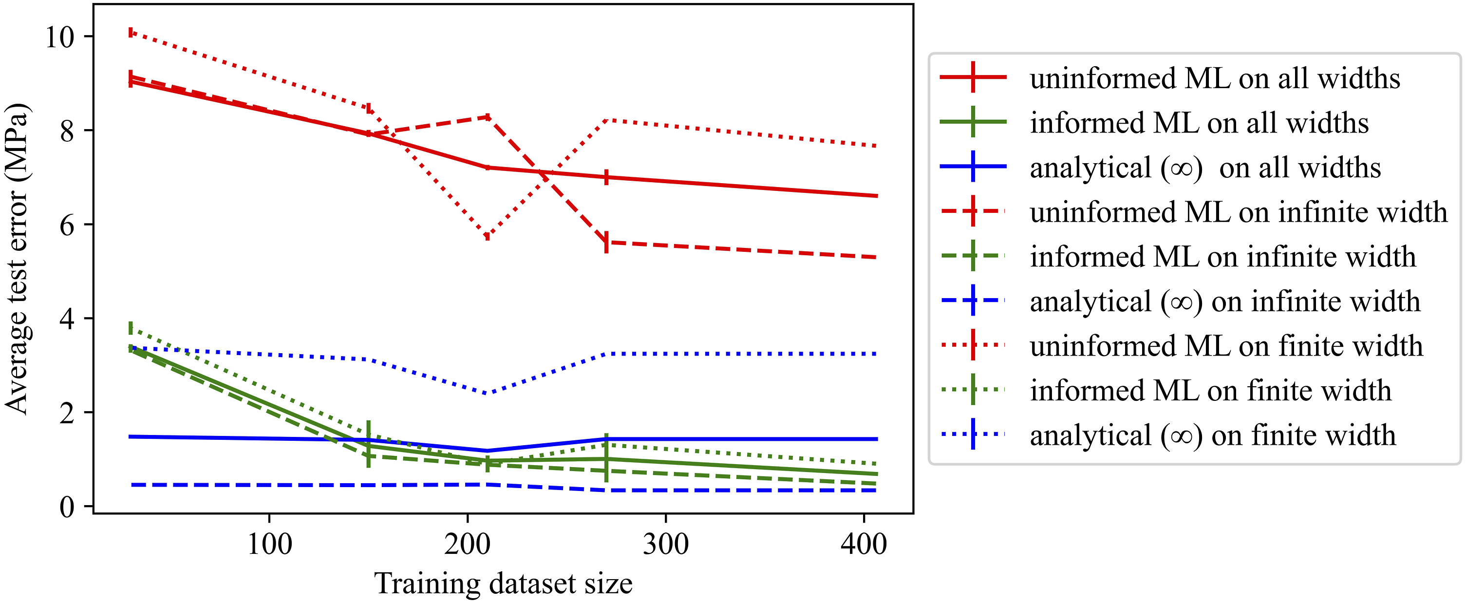

Effect of width and prediction method on maximum test error

In Table 2, we evaluate the maximum test error on stress predictions made by the analytical solution, the uninformed machine learning methodology and the analytical solution-informed machine learning methodology. Maximum test error is defined as the maximum error to the stresses predicted by FEA for the net section planes of laminates in the test dataset. The maximum amount of 406 dataset samples was used in this comparison.

Table 2.

Maximum test error for prediction methods for varying FWF.

	Maximum test error (MPa)
	Uninformed ML	Informed ML	Analytical (∞)
Infinite width (FWF = 10)	449.6	46.8	39.2
Finite width (FWF = 3)	416.9	59.5	127.7

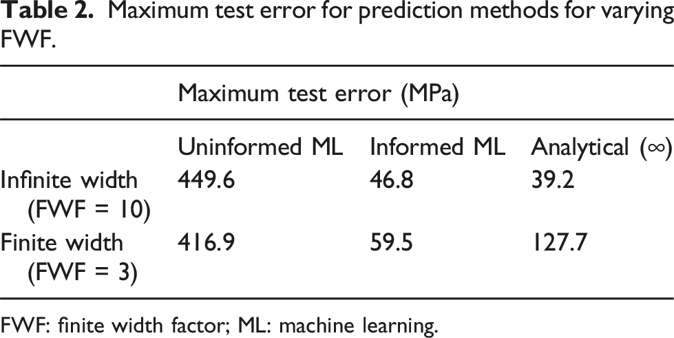
FWF: finite width factor; ML: machine learning.

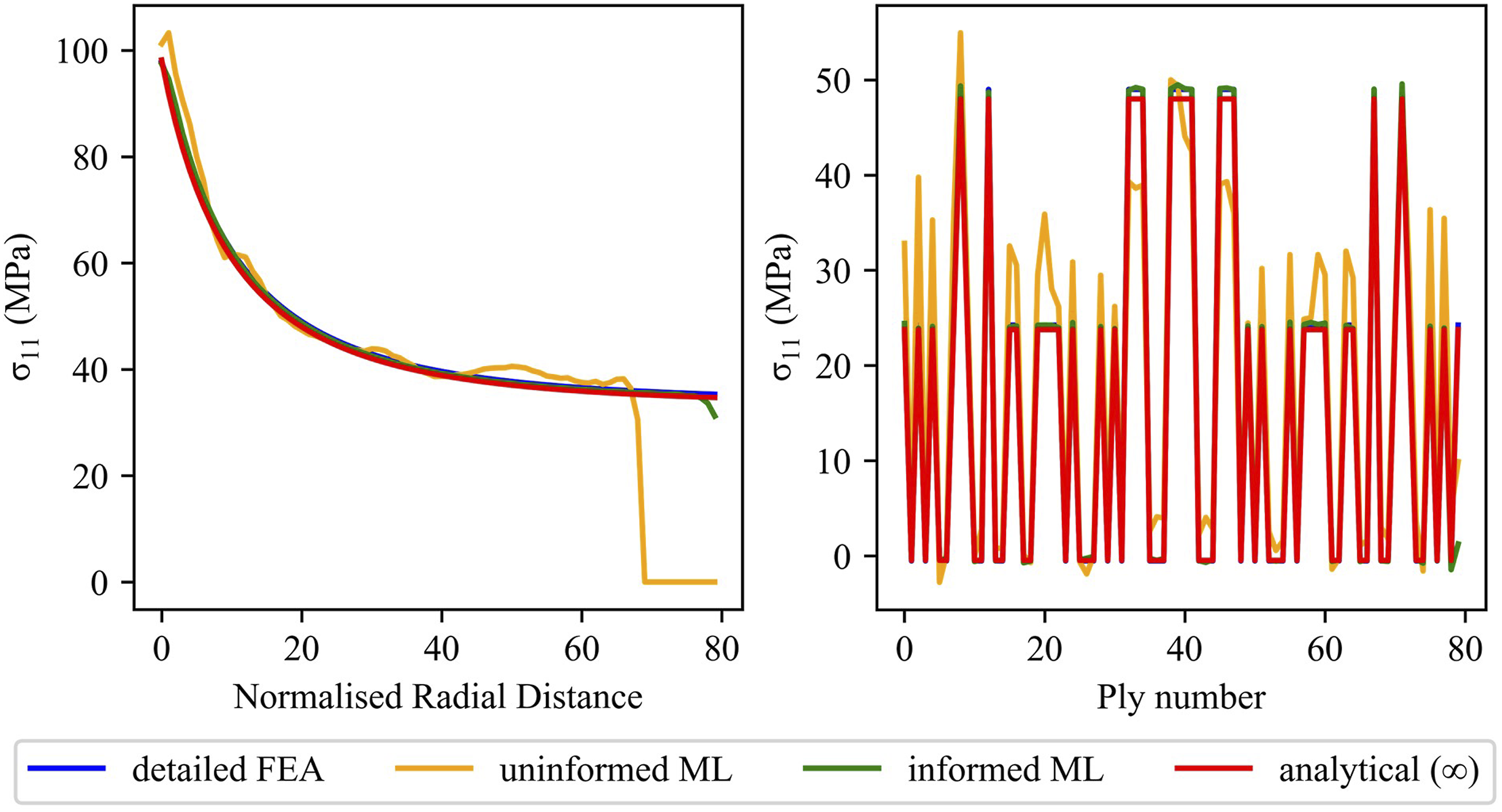
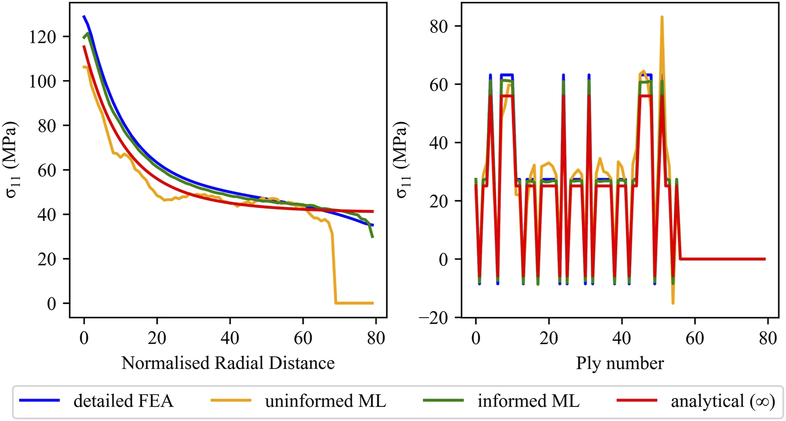
Through-thickness and radial stress distribution predictions

In this section, we compare the analytical solution predictions, uninformed machine learning predictions and analytical solution-informed ML predictions of net section stresses. The errors between such predictions to the FE stresses are shown for an example laminate in Figure 5. In this figure, multiple stress components are displayed for a comprehensive analysis. For further detail, this comparison is done radially away from the hole boundary (with radial distances normalised up to 2 × hole radius) for a given ply, and also through-thickness for all plies at a given distance (0.5 × radius) from the hole boundary. In Figure 6 we compare predictions made for an infinite-width plate, whereas in Figure 7 we compare predictions made for a finite-width (factor 3) plate.

Figure 5.

Example stress prediction errors for multiple stress components across the net section plane for a finite-width plate (with an additional key to show the ply angle for a given ply).

Figure 6.

Example stress distribution predictions for an infinite-width plate.

Figure 7.

Example stress distribution predictions for a finite-width plate.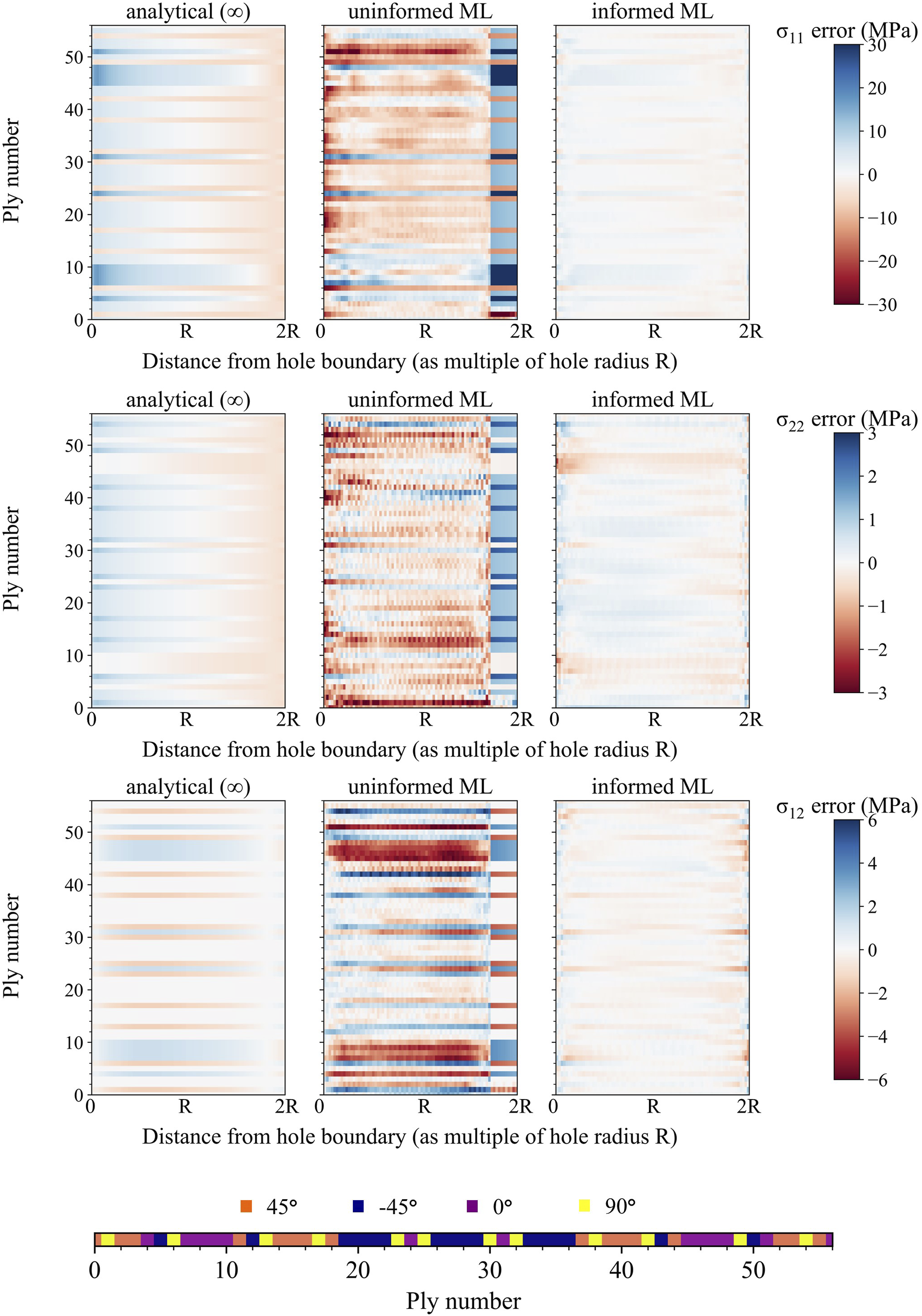

Application to global-local submodelling framework

Finally, we evaluate the use of the different prediction methods in a global-local context. We load a global model, with an average element length of 8 mm, by given membrane unit loads. Using the analytical solution, we can determine the expected loads if the plate is infinite in width. However, in a global-local modelling context, these loads would be unknown to the analyst. Therefore, we interrogate forces on the boundary of a local area of interest, with a central hole, to determine the far-field loading that was applied.

We use our modified Tan methodology to re-scale our predictions given interrogated loads towards predictions given expected loads. This can therefore be used to inform the analytical solution-informed machine learning model. The predictions made by this corrected machine learning model can be compared to predictions made by the commonly used Tan methodology. These comparisons are done under uniaxial loading $(N_{x} = 100 N / mm)$ and under biaxial loading $(N_{x} = 100 N / mm, N_{y} = 80 N / mm, N_{x y} = 60 N / mm)$ in Figure 8.

Figure 8.

Comparison of stress distributions in a given 0° ply. (a) Uniaxial loading (b) biaxial loading.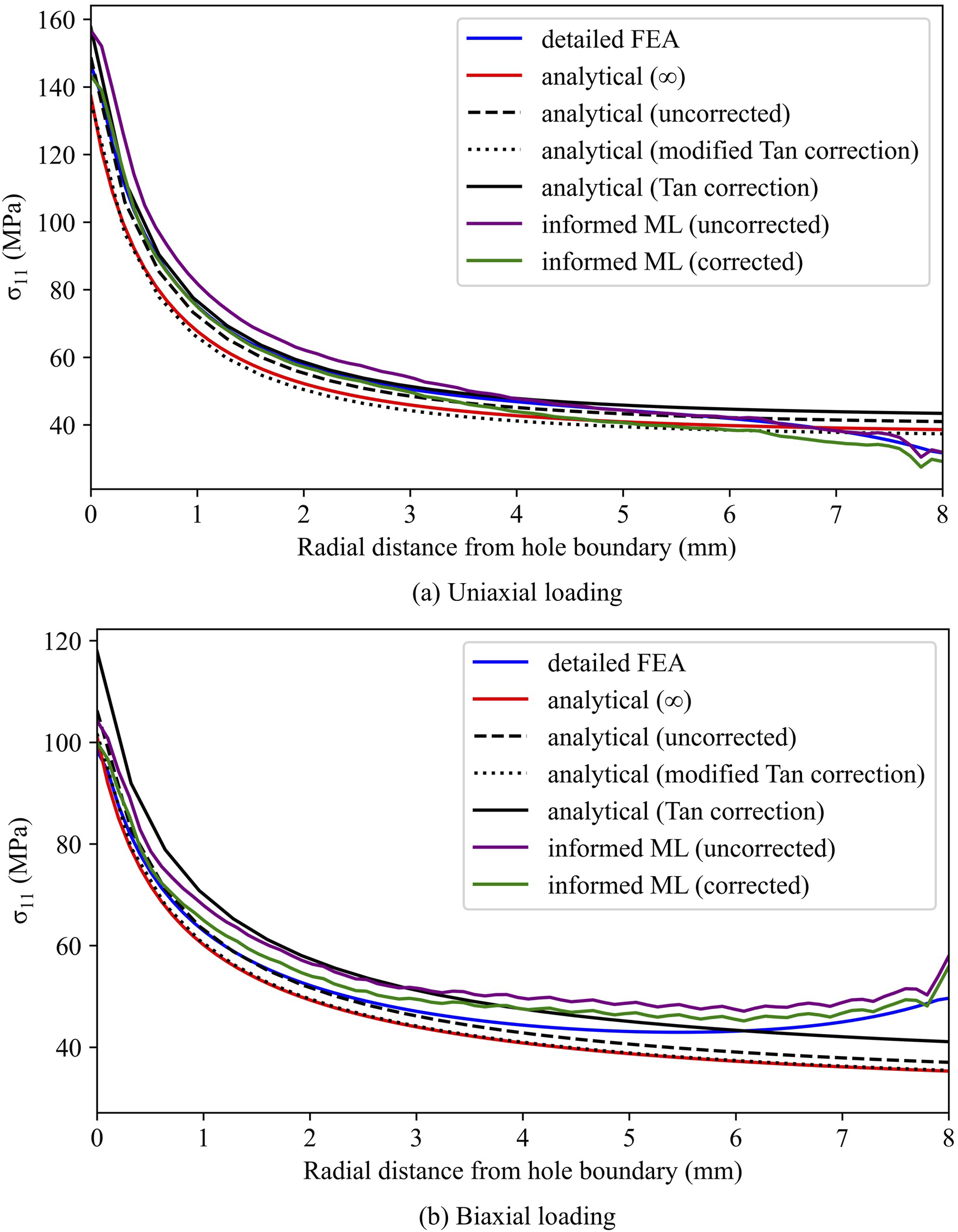

In Figure 9(a), we evaluate the distributions and predictions with further stress components. In Figure 9(b), we compare the effect of hole radius and laminate thickness on FE stress distributions and ML predictions. Laminate 1 has a 4 mm radius hole and is 5 mm thick, and laminate 2 has a 1 mm radius hole and is 7.5 mm thick.

Figure 9.

Performance of informed ML model on further testing. (a) Performance of informed ML for further stress components (b) effect of varying hole radius and laminate thickness on informed ML and detailed FEA. ML: machine learning; FEA: finite element analysis.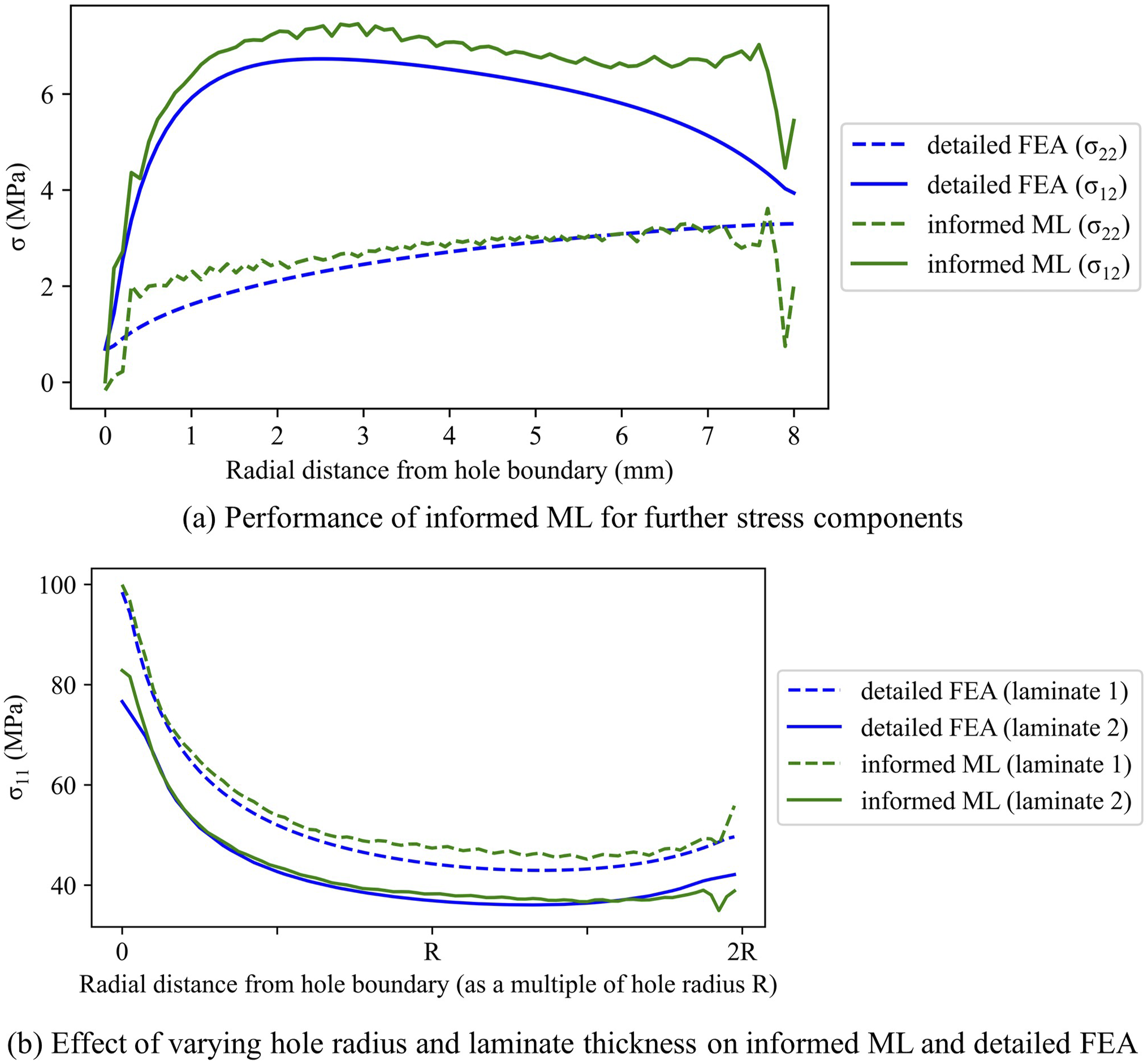

In Figure 10, we compare the total wall clock time made by different steps in the process of the stress analysis methods in this study. Both FE and ML analyses were run with 4 CPUs.

Figure 10.

Comparison of simulation time for different stress analysis methods.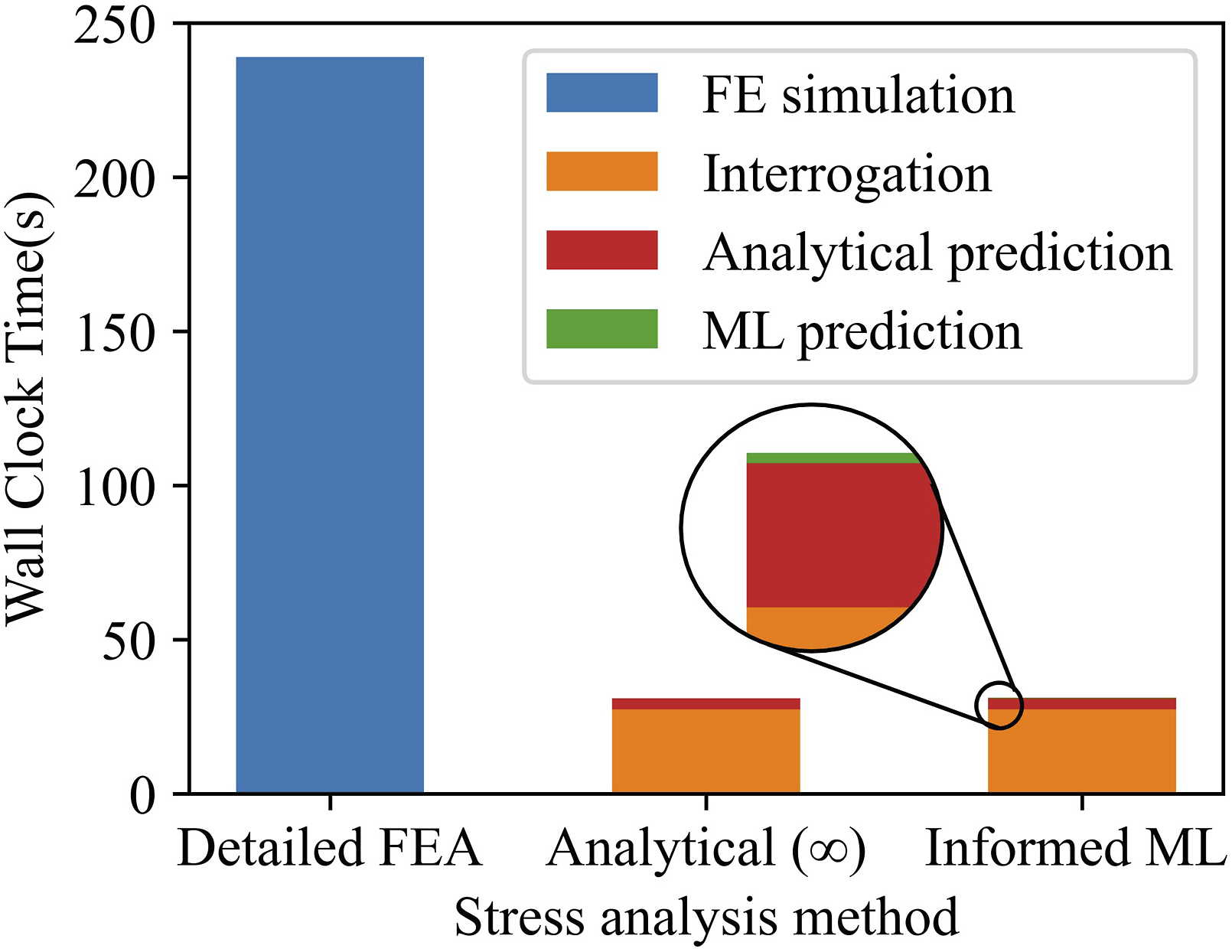

Discussion

In all cases analysed, for the dataset sizes investigated, the error has not yet converged, see Figure 4. Therefore, errors may be expected to improve further with more training data. However, we suggest that the ML performance will not exceed that of the analytical method on the infinite-width samples, as this is the theoretical minimum error of FE data to the analytical method.

As we can observe in Figure 4, the analytical solution-informed machine learning model performs significantly better than the uninformed machine learning model, across all widths. Given >400 samples, the uninformed ML model is still outperformed by an informed ML model with <50 samples. In Table 2, we can observe that the uninformed ML model is 9-10 times less accurate than other prediction methods. In Figures 6 and 7 the uninformed model shows unsatisfactory radial and through-thickness stress prediction, as neither the magnitude nor distribution of stresses match the detailed FEA results. In Figure 5 we further observe the uninformed neural network shows the largest errors in all stress components across the net section plane. Therefore, we can conclude that analytical information significantly improves the prediction accuracy of our ML model. Reducing the complexity of the additional analytical information, via an autoencoder, for example, may also be considered to further improve model accuracy.^27,28

When comparing errors for infinite-width predictions see Figure 4, the error from the analytical solution informed ML model approaches that of the analytical solution with increasing dataset size. We also see in Table 2 that the maximum test error for the informed ML model is similar to that of the analytical solution. From Figure 6, we find that the uninformed model achieves unsatisfactory prediction, whereas the informed ML model is able to closely match the radial and through-thickness distributions of the detailed FEA. We note that the informed ML model deviates from the FEA at the outermost radius. This may be due to the convolutional window sizes used in the neural network. Further hypertuning and increasing dataset size may be considered to remove this deviation, and further reduce error. However, overall, we can conclude that our informed ML model is able to perform as accurately as the analytical solution for infinite-width plates, given >400 training samples.

For finite-width plates, we can observe in Figure 4 that the informed ML model outperforms the analytical solution after ∼50 training samples. The maximum test error for the informed ML model is 47% of that of the analytical solution for the maximum training dataset size, see Table 2. As from Figure 5, the informed ML achieves lower errors overall than the analytical solution for 2D stress components across the net section plane. This is especially clear for stresses in the 11-direction. The magnitude of errors in this direction is higher due to the high fibre stiffness resulting in much higher stresses than in other components. From Figure 7, we further observe that, apart from the extremes in radius which may suffer deviations due to convolutional window size, the informed ML better captures the change in magnitude and distribution of stresses due to finite-width loading. Therefore, we conclude that our informed ML model is able to improve the analytical solution predictions to consider finite-width effects, given >150 training samples.

Under a global-local modelling context, as seen in Figure 8, we can observe that finite-width effects raise stress from the analytical solution of the infinite-width plate towards the detailed FEA results. This explains why the uncorrected analytical solution given interrogated loadings is higher than the infinite-width analytical solution. The use of a Tan factor on the uncorrected analytical solution raises stress accordingly, however, the distribution of stresses changes under finite-width effects and this Tan correction is unable to capture this.

Instead, we can see that our modified Tan correction is able to correct our uncorrected analytical solution given interrogated loads. As the global model has a significantly higher average element length, we see that despite our modified Tan correction the stress distribution slightly differs from the expected infinite-width analytical solution. The low fidelity modelling at the global level, results in the hole not being accurately represented and therefore the stiffness of the model in the local area results in inaccurate boundary forces. This is an artefact of the global-local modelling process, and a reminder that the global representation of the design feature affects the accuracy of stress predictions in its vicinity in the local model. However, our interrogation method is able to successfully capture a reasonable approximation of the stress distribution in a global-local context. Methods to more accurately capture stiffness despite low mesh density global modelling may be used to further reduce related errors.²⁹

For uniaxial loading, the mean absolute error of the Tan method to the detailed FEA results is 2.93%, whereas the mean absolute error of our informed ML methodology (without correction) increases to 3.30%. Combination of our modified Tan correction with our informed ML model results in a reduction of mean absolute error to 1.94%. For the case of biaxial loading, we see that our informed ML model shows further improvement in performance to traditional heuristic Tan scaling. The mean absolute error of the Tan method is 4.22%, whereas the mean absolute error of our informed ML methodology (without correction) is similar at 4.32%. Combination of our modified Tan correction with our informed ML model results in a reduction of mean absolute error to 1.77%. In this biaxial case, transverse and shear loads result in significant changes to stress distributions, which the Tan method is unable to capture. Overall, across loading, the use of the analytical solution with modified Tan correction to inform our ML model results in predictions that better capture the change in stress distribution due to finite-width effects. From Figure 9(a), we see that our informed ML methodology yields reasonable predictions across 2D stress components. Generally, it is observed that ML predictions in the radial direction can be discrete and irregular, as compared to the continuous FE and analytical predictions. Therefore, to further improve the accuracy of the ML model, a post-processing step involving smoothing such stress distributions may be considered.

As visible in Figure 9(b), the magnitude of stresses differs between laminates of varying thickness and hole radius. The greater the laminate thickness, the greater the cross-sectional area, and therefore the lower the net-section stresses for a given unit force. However, the distributions of stresses and predictions do not change greatly. It is the finite width factor which plays the most importance in distributions, not the hole radius itself. The effects of finite width factor are shown in Figures 5–7.

Finally, from Figure 10, we observe that our informed ML prediction is performed nearly as fast as the analytical solution, and both methods offer a 6-fold time-saving benefit to the detailed FEA model. The time to run the ML model itself is in the order of ∼200 ms and so is of negligible concern as an addition to the time to run the analytical solution. The longest time for both analytical solutions and informed ML models is the interrogation time. This includes the time to run the root-finding analyses to convert interrogated boundary forces to remote loads, as well as the time to compute (modified) Tan corrections. While our informed ML method shows a 200 s improvement to traditional detailed FEA methods, this saving is expected to compound given thousands of such features exist in an airframe, and for optimisation studies further orders of magnitude of runs may be required. For a large scale structure with a thousand features, for example, the nominal CPU time-saving benefit of our methodology is over 220 h. ML models make fast and scalable predictions using simple matrix operations. Therefore, for more complex features than open holes, which require longer FE simulations, the time-saving benefit of our methodology would further increase. This would be the case for bolted joints for example, which have a similar analytical solution ⁷ but require longer FEA simulation times due to higher fidelity meshing, larger model size and consideration of contact.³⁰

For composite structures with non-circular hole boundaries, modifications may be required to the underlying analytical method using methods from previous studies.^31,32 Our methodology is used to investigate the stresses around a singular hole. For multiple holes, hole interaction effects are minimised by following design guidelines,²⁰ and so are neglected in this methodology. Our methodology is applicable for static analyses, as for the early validation stages of airframe design, for example. Dynamic effects are therefore neglected. To account for local variations in composite layup, material discontinuities and manufacturing defects, we suggest parameterising such variations and including these variations in the training data.

Conclusions

In this study, we have used the analytical solution for an infinite-width plate under membrane loading to inform convolutional neural network-based predictions for finite-width analyses within a global-local modelling context.

We have found that our informed ML model performs significantly more accurately than an uninformed ML model. The informed ML model performs as accurately with less than 50 samples as the uninformed model with greater than 400 samples. We find that the informed ML model approaches the accuracy of the analytical solution for infinite-width plates and outperforms this solution for finite widths. We find that the informed ML model also outperforms heuristic-based Tan corrections for finite-width correction, as it is better able to capture the change in stress distributions under finite-width effects.

In a global-local submodelling context, our modified Tan correction is able to improve our informed ML model predictions, by considering errors made in calculating remote loads following interrogation of loads on the boundary of the local area of interest in the global model. Our model demonstrates accuracy benefits under both uniaxial loading and biaxial loading. We also show a 6-fold time-saving benefit of our informed ML model over traditional detailed FE submodelling, and a negligible addition to simulation time as compared to the analytical solution.

Overall, our informed ML model results in fast, high-accuracy predictions given reduced training dataset sizes for both infinite-width and finite-width plates. This methodology can in principle be applied to a variety of structural components including, for instance, both bearing and bypass situations for a bolted composite joint.

Footnotes

Acknowledgements

The first author acknowledges funding from the Department of Aeronautics, Imperial College London. The second author acknowledges funding from EPSRC project EP/W022508/1. The authors express gratitude and remembrance of the kind support and supervision of the late Professor Lorenzo Iannucci.

Declaration of conflicting interests

The author(s) declared no potential conflicts of interest with respect to the research, authorship, and/or publication of this article.

Funding

The author(s) disclosed receipt of the following financial support for the research, authorship, and/or publication of this article: This work was supported by EPSRC (No. EP/W022508/1).

ORCID iD

Omar Ahmed Imran Azeem

Data availability statement

Data will be made available upon request.*

References

Kassapoglou

. Holes. In: Modeling the effect of damage in composite structures: simplified approaches. Chichester: Wiley, 2015, pp. 9–40.

Hart-Smith

. Mechanically-fastened joints for advanced composites — phenomenological considerations and simple analyses. In: Fibrous composites in structural design. Boston, MA: Springer, 1980, pp. 543–574.

Waszczak

Cruse

. Failure mode and strength predictions of anisotropic bolt bearing specimens. J Compos Mater 1971; 5: 421–425.

Whitney

Nuismer

. Stress fracture criteria for laminated composites containing stress concentrations. J Compos Mater 1974; 8: 253–265.

Chang

Scott

Springer

. Strength of mechanically fastened composite joints. J Compos Mater 1982; 16: 470–494.

Lekhnitskii

. Anisotropic plates. https://apps.dtic.mil/sti/citations/AD0683218 (1968, accessed 10 December 2023).

HyperSizer . Bolted joint analyses. https://hypersizer.com/help_7.0/Content/Failure/BJSFM/bjsfm-about.php (2014, accessed 10 December 2023).

Tan

. Finite-width correction factors for anisotropic plate containing a central opening. J Compos Mater 1988; 22: 1080–1097.

de Jong

. Stresses around pin-loaded holes in elastically orthotropic or isotropic plates. J Compos Mater 1977; 11: 313–331.

10.

Nguyen-Hoang

Becker

. Open holes in composite laminates with finite dimensions: structural assessment by analytical methods. Arch Appl Mech 2022; 92: 1101–1125.

11.

Pastorino

Blázquez

López-Romano

, et al. Closed-form methodology for stress analysis of composite plates with cutouts and non-uniform lay-up. Compos Struct 2019; 212: 389–397.

12.

Freed

. Implementation of machine learning strategies for determination of finite width correction factors for orthotropic plates containing central hole. J Compos Mater 2022; 56: 4221–4230.

13.

Krokos

Bui Xuan

Bordas

SPA

, et al. A Bayesian multiscale CNN framework to predict local stress fields in structures with microscale features. Comput Mech 2022; 69: 733–766.

14.

Bhaduri

Gupta

Graham-Brady

. Stress field prediction in fiber-reinforced composite materials using a deep learning approach. Compos B Eng 2022; 238: 109879.

15.

Yang

Buehler

. Deep learning model to predict complex stress and strain fields in hierarchical composites. Sci Adv 2021; 7: eabd7416.

16.

Azeem

OAI

Pinho

. A machine learning assisted multifidelity modelling methodology to predict 3D stresses in the vicinity of design features in composite structures. Int J Solids Struct 2024; 301: 112946.

17.

GitHub - BenjaminETaylor/bjsfm . Bolted joint stress field model. https://github.com/BenjaminETaylor/bjsfm (accessed 15 December 2023).

18.

Ahrens

Geveci

Law

. Paraview: an end-user tool for large data visualization. Visualization Handbook: Elsevier, 2005.

19.

Dassault Systemes . Abaqus standard. https://www.3ds.com/(2021, accessed 15 December 2023).

20.

Abbot

. Analysis and design of composite and metallic flight vehicle structures. Grand Cayman: Abbot Aerospace, 2017.

21.

Abadi

Barham

Chen

, et al. TensorFlow: a system for large-scale machine learning.

22.

Chollet

. Keras 2015. https://keras.io (accessed 15 December 2023).

23.

Ronneberger

Fischer

Brox

. U-net: convolutional networks for biomedical image segmentation. Lect Notes Comput Sci 2015; 9351: 234–241.

24.

Virtanen

Gommers

Oliphant

, et al. SciPy 1.0: fundamental algorithms for scientific computing in Python. Nat Methods 2020; 17: 261–272.

25.

De Saint-Venant

. Mem. Acad. Sci Savants etrangers. De la torsion des prismes 1855; 14: 233–560.

26.

Niu

. Composite airframe structures practical design information and data. Hong Kong: Conmilit Press Limited, 1992.

27.

Bolón-Canedo

Remeseiro

. Feature selection in image analysis: a survey. Artif Intell Rev 2020; 53: 2905–2931.

28.

Kabir

Garg

. Machine learning enabled orthogonal camera goniometry for accurate and robust contact angle measurements. Sci Rep 2023; 13: 1–13.

29.

Reille

Champaney

Daim

, et al. Learning data-driven reduced elastic and inelastic models of spot-welded patches. Mechanics & Industry 2021; 22: 32.

30.

Egan

McCarthy

, et al. Stress analysis of single-bolt, single-lap, countersunk composite joints with variable bolt-hole clearance. Compos Struct 2012; 94: 1038–1051.

31.

Hsieh

Hwu

. A full field solution for an anisotropic elastic plate with a hole perturbed from an ellipse. Eur J Mech Solid 2023; 97: 104823.

32.