Review of elasto-static models for three-dimensional analysis of thick-walled anisotropic tubes

Abstract

Most shell or beam models of anisotropic tubes under bending have no validity for thick-walled structures. As a result, the need to develop three-dimensional formulations which allow a change in the stress, strain and displacement distributions across the radial component arises. Basic formulations on three-dimensional anisotropic elasticity were made either stress- or displacement-based by Lekhnitskii or Stroh on plates. Lekhnitskii also was the first to expand these analytical formulations to tubes under various loading conditions. This paper presents a review of the stress and strain analysis of tube models using three-dimensional anisotropic elasticity. The focus lies on layered structures, like fiber-reinforced plastics, under various bending loads, although the basic formulations and models regarding axisymmetric loads are briefly discussed. One section is also dedicated to the determination of an equivalent bending stiffness of tubes.

Introduction

This paper provides a review of analytical and semi-analytical models and enhancements for the three-dimensional analysis of stresses, strains and displacements of cylindrical tubes with linear-elastic, anisotropic material behavior. Since the main focus is on composite materials and their multi-layer design, special cases of material symmetry like monotropy, orthotropy and transverse-isotropy are considered. In general, all formulations are basicly developed for a single-layered tube and the layering is achieved by a multiple use of the model description and fulfillment of continuity conditions at the interphases. Even though the material description is three-dimensional, the stress and strain distributions are usually functions of only one or two coordinate directions to obtain a solvable system of governing equations. However, there are models with approximate solutions for the remaining dimensions using a series expansion or numeric methods.

The tube is globally described by a cylindrical coordinate system, where the principal directions are called radial r, circumferential θ and axial z, as well as a cartesian coordinate system x, y and z. As illustrated in Figure 1, both have their origin in the center of the circular cross section. Therefore, x- and y-positions could be expressed as x = r sin φ and y = r cos φ. In some cases a third global coordinate system is established, with the only difference being that the radial component, later refered to as $\stackrel{\sim }{r}$ , originates in the center of the laminate and not the tube cross-section. The associated displacements are indicated as u _x , u _y , u _z or rather u, v, w for cartesian coordinates and as u _r , u _θ , u _z for cylindrical coordinates, respectively. Stresses and strains are described by the related 3×3 tensor, which could be transferred to a 6×1 vector in notation by Voigt, ¹ for the cylindrical coordinate system.

Figure 1.

General cartesian and cylindrical coordinate systems of the tube used according to the definition of Lekhnitskii ² and the local and global cartesian coordinate system of the material in the wound fiber-reinforced tube with specification of the angle definition for the transformation of the material properties from the ply to laminate.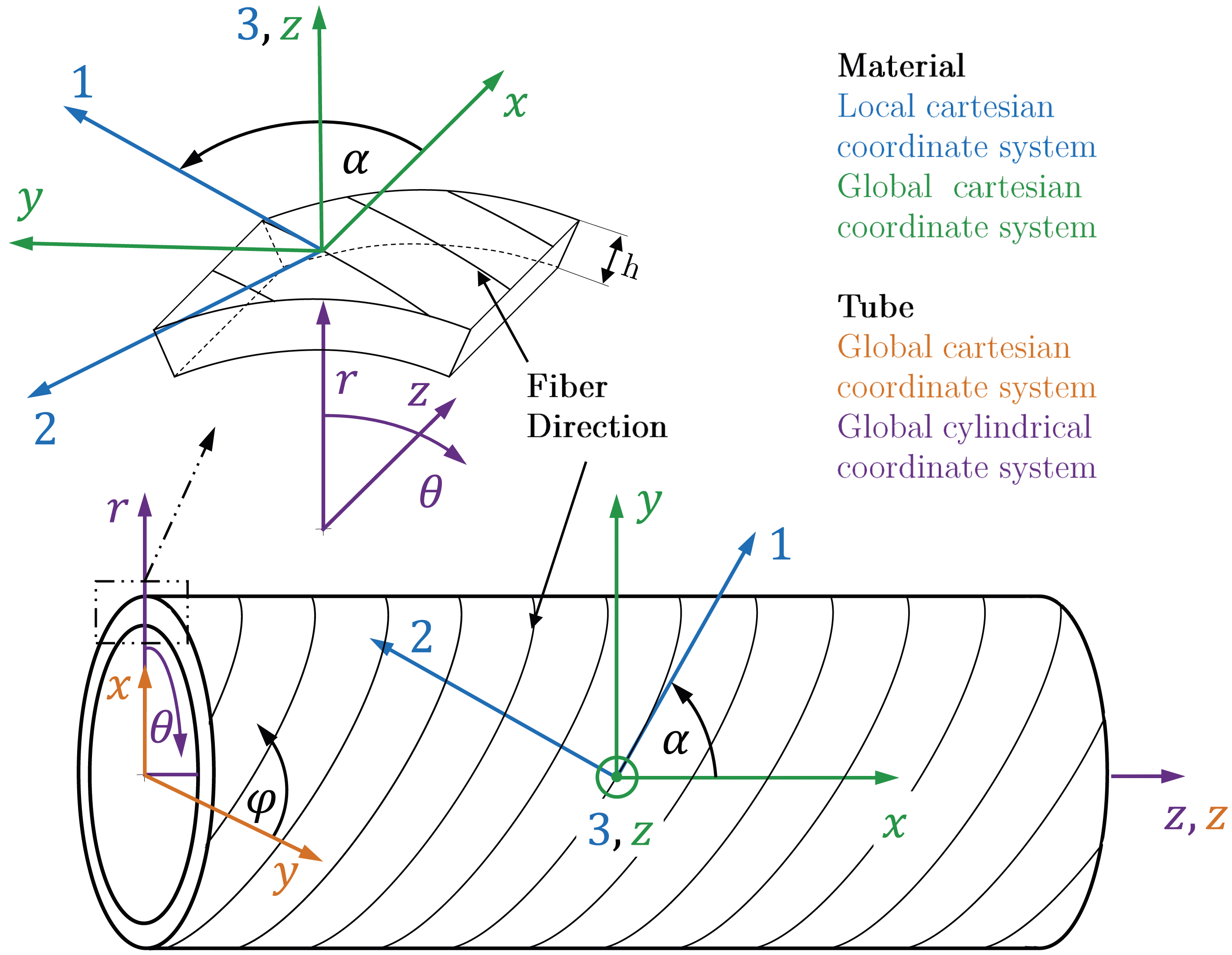

It should be noted here that the global cartesian tube coordinate system in Figure 1 is taken from the basic definition of Lekhnitskii, ² who defines the basis for further bending models. For the material description, however, the local and global coordinate systems must be used to ensure a consistent transformation of the ply to laminate properties. For the transformation from the global cartesian laminate coordinate system to the cylindrical tube coordinate system according to Lekhnitskii, ² reference should be made to Siegl and Ehrlich, ³ who ensure the use of the correct transformed material parameters for the use of tube bending models via an introduced permutation matrix. Lekhnitskii ² relates his cartesian coordinate system to generally anisotropic materials and does not take into account the fiber orientation, which according to his definition would lie in the radial direction in the tube cross-section and thus has no technical application. ³ If consistent coordinate systems for the material description as well as of the global tube based on the fiber orientation is desired, reference should be made to Almeida et al., ⁴ nevertheless the relations of Lekhnitskii (1963) are necessary to use the bending models, which is why they are used in this paper.

The considered load types for the static analysis are differentiated into axisymmetric and antisymmetric loads. The former includes axial tension and compression, internal and external pressure, torsion as well as in-plane shearing, the latter mainly consists of bending, transverse shearing and local transverse load. This review is focusing on tubes subjected to different bending loads and boundary conditions, but will also give an overview of general formulations regarding three-dimensional anisotropic elasticity and tubes under axisymmetric loads. Even though, some models in this review are capable of enabling dynamic analyses due to the physical description in form of an eigenvalue problem, it is focused on models under static and mechanical loads. Three-dimensional anisotropic elasticity also implies that the tubes are thick-walled and shell or beam formulations are not considered. A distinction between thin-walled and thick-walled tubes is made by the ratio of radius to thickness, which is strongly dependend on the used material and load case.

Constitutive law

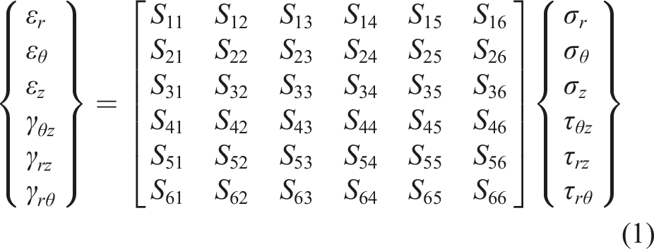
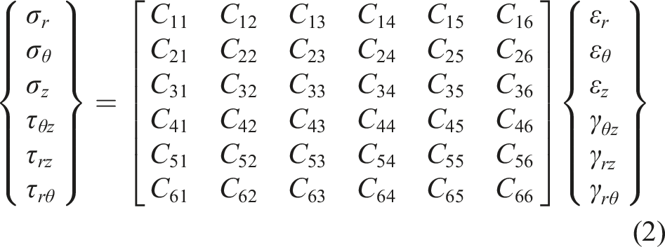
Regardless of the respective model or approach, the continuum is described by three fundamental equations: constitutive law, equilibrium equations and kinematic relationships. In case of a cylindrical tube, the general anisotropic material law in global form becomes

$\left\{\begin{array}{l}{\epsilon }_r\\ {\epsilon }_{\theta }\\ {\epsilon }_z\\ {\gamma }_{\theta z}\\ {\gamma }_{rz}\\ {\gamma }_{r\theta }\end{array}\right\}=\left[\begin{array}{llllll}{S}_{11}& S_{12}& S_{13}& S_{14}& S_{15}& S_{16}\\ S_{21}& S_{22}& S_{23}& S_{24}& S_{25}& S_{26}\\ S_{31}& S_{32}& S_{33}& S_{34}& S_{35}& S_{36}\\ S_{41}& S_{42}& S_{43}& S_{44}& S_{45}& S_{46}\\ S_{51}& S_{52}& S_{53}& S_{54}& S_{55}& S_{56}\\ S_{61}& S_{62}& S_{63}& S_{64}& S_{65}& S_{66}\end{array}\right]\left\{\begin{array}{l}{\sigma }_r\\ {\sigma }_{\theta }\\ {\sigma }_z\\ {\tau }_{\theta z}\\ {\tau }_{rz}\\ {\tau }_{r\theta }\end{array}\right\}$

(1)

or

$\left\{\begin{array}{l}{\sigma }_r\\ {\sigma }_{\theta }\\ {\sigma }_z\\ {\tau }_{\theta z}\\ {\tau }_{rz}\\ {\tau }_{r\theta }\end{array}\right\}=\left[\begin{array}{llllll}{C}_{11}& C_{12}& C_{13}& C_{14}& C_{15}& C_{16}\\ C_{21}& C_{22}& C_{23}& C_{24}& C_{25}& C_{26}\\ C_{31}& C_{32}& C_{33}& C_{34}& C_{35}& C_{36}\\ C_{41}& C_{42}& C_{43}& C_{44}& C_{45}& C_{46}\\ C_{51}& C_{52}& C_{53}& C_{54}& C_{55}& C_{56}\\ C_{61}& C_{62}& C_{63}& C_{64}& C_{65}& C_{66}\end{array}\right]\left\{\begin{array}{l}{\epsilon }_r\\ {\epsilon }_{\theta }\\ {\epsilon }_z\\ {\gamma }_{\theta z}\\ {\gamma }_{rz}\\ {\gamma }_{r\theta }\end{array}\right\}$

(2)

in notation of the compliances [S _ij ] or stiffnesses $\left[C_{ij}\right]={\left[S_{ij}\right]}^{-1}$ with i, j = 1-6. Due to the presence of a symmetry plane and the reflection of all characteristic values on it, the stiffness and compliance matrices can be simplified to a monotropic or monoclinic material behavior. The compliance matrix, as an example, is then expressed by

$\left[S_{ij,\text{mono}}\right]=\left[\begin{array}{llllll}{S}_{11}& S_{12}& S_{13}& S_{14}& 0& 0\\ S_{21}& S_{22}& S_{23}& S_{24}& 0& 0\\ S_{31}& S_{32}& S_{33}& S_{34}& 0& 0\\ S_{41}& S_{42}& S_{43}& S_{44}& 0& 0\\ 0& 0& 0& 0& S_{55}& S_{56}\\ 0& 0& 0& 0& S_{65}& S_{66}\end{array}\right].$

(3)

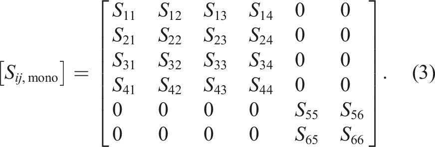
If a second or even third symmetry plane exists orthogonal to the first one, a further simplification to orthotropic material behavior is possible and

$\left[S_{ij,\text{ortho}}\right]=\left[\begin{array}{llllll}{S}_{11}& S_{12}& S_{13}& 0& 0& 0\\ S_{21}& S_{22}& S_{23}& 0& 0& 0\\ S_{31}& S_{32}& S_{33}& 0& 0& 0\\ 0& 0& 0& S_{44}& 0& 0\\ 0& 0& 0& 0& S_{55}& 0\\ 0& 0& 0& 0& 0& S_{66}\end{array}\right].$

(4)

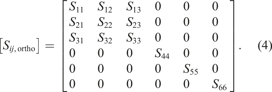
A material is called transversely isotropic or in some literature cylindrically anisotropic, if there are infinite symmetry planes around one coordinate direction. The matrix occupancy does not change in comparison to orthotropy, but the individual entries can be expressed by less characteristic values. The elastic state of the material can be expressed by 13 independent mechanical properties in case of monotropy, 9 in case of orthotropy and 5 in case of transversely isotropy. Note that there are many different notations for constitutive law and, in particular, the compliances in the literature.

Equilibrium Equations

The equilibrium equations are derived using the cartesian coordinate system for cylindrical stresses under the assumption of small angles on a segment of the hollow cylinder. On the basis of these assumptions, the curved surfaces of the segment can be approximated by plane surfaces and the cross section becomes trapezoidal. For all stresses, a Taylor series expansion is applied according to σ _r (r) = σ _r and σ _r (r + dr) = σ _r + (∂σ _r /∂r) dr. All terms multiplied by the finite dimensions dr, dθ or dz can be neglected because of the low values. By also neglecting inner forces of the continuum, the equilibrium equations result to

$\begin{array}{l}\frac{\partial {\sigma }_r}{\partial r}+\frac{1}{r}\hspace{1em}\frac{\partial {\tau }_{r\theta }}{\partial \theta }+\frac{\partial {\tau }_{rz}}{\partial z}+\frac{{\sigma }_r-{\sigma }_{\theta }}{r}=0,\\ \frac{\partial {\tau }_{\theta r}}{\partial r}+\frac{1}{r}\hspace{1em}\frac{\partial {\sigma }_{\theta }}{\partial \theta }+\frac{\partial {\tau }_{\theta z}}{\partial z}+\frac{2{\tau }_{\theta r}}{r}=0,\\ \frac{\partial {\tau }_{zr}}{\partial r}+\frac{1}{r}\hspace{1em}\frac{\partial {\tau }_{z\theta }}{\partial \theta }+\frac{\partial {\sigma }_z}{\partial z}+\frac{{\tau }_{zr}}{r}=0.\end{array}$

(5)

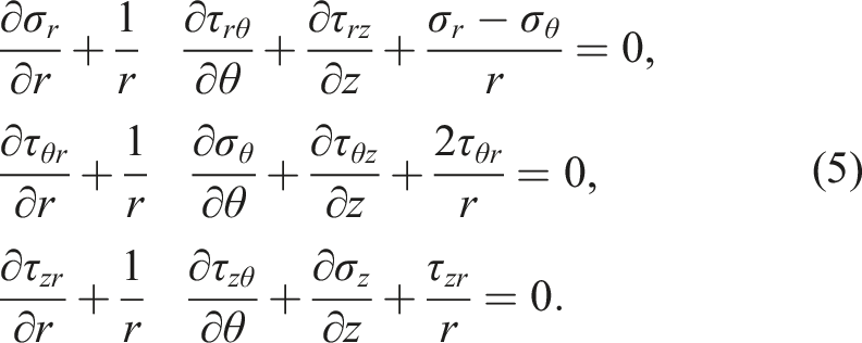
The indices ij (i, j = r, θ, z) correspond to the notation of the section plane i and the direction of action j. Equation (5) are describing the general form of equilibrium equations. In dependence of the specific model the stresses are independent of one or two coordinates, thus eliminating the derivatives in the respective directions.

Kinematic relationships

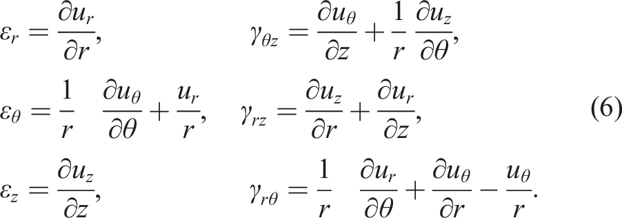
The strains can be distinguished in normal strains {ɛ _i } and shear strains {γ _ij } for i, j = r, θ, z. Mathematically, they are described by changes in the length and angular ratios of the continuum, which can be expressed in terms of displacements. Due to the contiguous ring cross-section of the tube, a normal strain in tangential direction also produces an additional displacement in the radial direction. The kinematic relationships, in form of the strain-displacement relations, follow from vectorial considerations on a segment of the hollow cylinder with small-angle approximations, a Taylor series expansion according to the predescribed use for the stresses and the assumption that only a minimal change over the radius occurs. In general terms, they are

$\begin{array}{l}{\epsilon }_r=\frac{\partial u_r}{\partial r},\hspace{1em}\hspace{1em}\hspace{1em}\hspace{1em}\hspace{1em}{\gamma }_{\theta z}=\frac{\partial u_{\theta }}{\partial z}+\frac{1}{r} \frac{\partial u_z}{\partial \theta },\\ {\epsilon }_{\theta }=\frac{1}{r}\hspace{1em}\frac{\partial u_{\theta }}{\partial \theta }+\frac{u_r}{r},\hspace{1em}{\gamma }_{rz}=\frac{\partial u_z}{\partial r}+\frac{\partial u_r}{\partial z},\\ {\epsilon }_z=\frac{\partial u_z}{\partial z},\hspace{1em}\hspace{1em}\hspace{1em}\hspace{1em}\hspace{1em}{\gamma }_{r\theta }=\frac{1}{r}\hspace{1em}\frac{\partial u_r}{\partial \theta }+\frac{\partial u_{\theta }}{\partial r}-\frac{u_{\theta }}{r}.\end{array}$

(6)

In equation (6) the derivatives for the respective directions disappear, if the strains and displacements are considered invariabel along these directions.

Further damage and failure-considering investigations

In addition to the elasto-static models for three-dimensional analysis of thick-walled anisotropic tubes summarised here in detail, there are also numerous analytical, numerical and experimental studies that deal with damage, failure and buckling of filament wound composite tubes for further load cases besides bending, as well as considering the aeroelasticity and buckling of plates that could be used for an application on fiber-reinforced tubes.

Further experimental, numerical and analytical studies on composite tubes under different loading scenarios

If, at higher loads, the material behaviour can no longer be adequately described with the linear-elastic approaches, reference should be made to the investigations on the damage and failure of filament wound tubes under different loading scenarios. Experimental and numerical approaches under external pressure loads are described in Almeida et al. ⁵ For radial compression of the composite tubes, damage modelling can be found in Almeida et al. ⁶ and the influence of the winding pattern of the composite tubes is described in Lisboa et al. ⁷ Based on genetic algorithm accounting progressive damage, Almeida et al. ⁸ developed an optimization of the stacking sequence of composite tubes under internal pressure. Regarding the internal pressure loading of the composite tubes, in Azizian and Almeida ⁹ surrogate models are used for stochastic, probabilistic and relaibility analyses have using artificial neural network metamodels. Further, optimisations and effects on the manufacturing of variable-angle composite cylinders can be obtained from experiments using digital image correlation (DIC) to capture the strains on composite tubes under axial compression in Almeida et al. ¹⁰ Here, the measurement of imperfections is also used to perform non-linear numerical model along with a progressive damage analysis to describe the occurring buckling mechanisms more precisely. Further findings and fundamentals on buckling of composite tubes under axial compression are presented in Almeida et al. ⁴ regarding buckling and post-buckling as linear, nonlinear, damage and experimental analysis and in Almeida et al. ¹¹ the basic design methodology for optimising the tube with variable-axial fiber layout can be found. Furthermore, in Wang et al. ¹² a reliability-based buckling optimisation with an accelerated kriging metamodel can be found for in the winding process using variable angles. Based on this, further developments of the Kriging-based metamodel in combination with particle swarm optimisation can be found in Wang et al. ¹³ Further insights into the compression of composite tubes can be found in Stedile Filho et al., ¹⁴ who also investigate the torsion load of the structure, which is used as a drive shaft. Furthermore, the influences of mosaic pattern on hygrothermally-aged composite tubes under axial compression have been investigated in Azevedo et al. ¹⁵

Further investigations on aeroelasticity and buckling of composite plates

Aeroelasticity considers the phenomena resulting from the interaction of aerodynamic (especially transient), inertial and elastic forces that occur during the relative motion of a fluid (air) and a flexible body (aircraft). ¹⁶ Based on the approaches to aeroelasticity and buckling of composite plates, certain material properties can be derived that can be used for further investigations on fiber-reinforced tubes that could be used in the aerospace industry. For this purpose, the recent studies by Sharma et al. ¹⁷ on stochastic frequency analysis of composite plates with curvilinear fiber and Sharma et al. ¹⁸ on stochastic aeroelastic analysis of laminated composite plates with variable fiber spacing can be considered. The aeroelastic analysis of plates made of lightweight materials with material uncertainty is described in Swain et al. ¹⁹ Methods for quantifying the uncertainty in the free vibration and aeroelastic response of an angularly adjustable laminates are given in Sharma et al. ²⁰ The aeroelastic control of delaminated angle tow laminated composite plates using piezoelectric patches is given in Sharma et al. ²¹ The use of piezoelectric patches is also described in the study by Sharma et al. ²² to investigate active flutter suppression of damaged variable stiffness laminated rectangular plate. Further investigations in the field of free vibration can be found in Sharma et al., ²³ who studied the static and free vibration analysis of smart variable stiffness composite plates with delaminations. On the other hand, in Sharma et al. ²⁰ a study is made for uncertainty quantification in free vibration and aeroelastic response of variable angle tow laminated composite plates. Uncertainty quantification under thermal loading in buckling strength of variable stiffness laminated composite plates can be found in Sharma et al. ²⁴ For functionally graded sandwich plates using layerwise theory, a vibration and certainty analysis has been carried out in Sharma et al. ²⁵

Three-Dimensional anisotropic elasticity

Three-dimensionality implies that the examined continua are thick-walled and thus their properties change in thickness direction. Theories which reduce the material properties of a laminate to its median plane are therefore excluded. Models regarding three-dimensional anisotropic elasticity can be distinguished into formulations using complex variables as well as formulations using the state-space approach. Although some of these theories provide exact solutions in all three coordinate directions for simple continua, most models need to limit the stresses, strains and displacements to functions of only one or two coordinates to obtain a solveable system of governing equations. Therefore, some approaches use approximate solutions along one, two or even all three directions.

General formulation using complex variables

There are two fundamental formulations of general anisotropic elasticity, the stress- or compliance-based according to Lekhnitskii ² and the displacement- or stiffness-based according to Stroh, ²⁶ Stroh ²⁷ and Eshelby et al. ²⁸ Both methods share similar approaches to describe the elastic state of the homogenous continuum, although different state variables are used. Constitutive law, equilibrium equations and strain-displacement relations are employed as fundamental equations to generate a system of governing equations. Stresses, strains and displacements are existent in three dimensions, but do not vary along one coordinate. For most of the tube models, there is no variation along the tube axis z.

General formulation by Lekhnitskii

Lekhnitskii ² is expressing the strains and displacements as functions of the stresses, which leads to the necessity of performing compatibility conditions for the three displacements of the motion field. By applying the stress functions of Airy and Prandtl, the stresses are reduced to two unknowns. A system of partial differential equations is formed for the unknown stress functions using the aforementioned fundamental equations in terms of reduced compliances as well as the geometrical parameters and their derivations. The solution is then obtained in form of a sixth order polynomial, the so-called sextic equation, by inserting predefined initial functions for the stress functions and a subsequent integration. Henceforth, it is possible to describe stresses, strains and displacements as functions of the unknown integration constants C _i (i = 1-6) in the polynominal equation, the compliances, reduced compliances and coordinate positions. For the respective load condition and continuum, simplifications of the fundamental equations can be made beforehand and the integration constants are determined through boundary conditions.

General formulation by Stroh

Stroh ²⁶ on the other hand operates with already compatible displacements of an arbitrary solid, that are independent of one dimension (here z) of an cartesian coordinate system (x, y, z). According to Eshelby et al. ²⁸ the compatible displacement vector {u _c } can be expressed by the summation of three complex functions composed of an unknown vector {A_c,i} and a function of an unknown complex coefficent p _i as well as the two dependent coordinates x and y with

$\left\{u_c\right\}={\displaystyle \sum }_{i=1}^3\left\{A_{c,i}\right\}\hspace{0.17em}f\left(x+p_i\hspace{0.17em}y\right),$

(7)

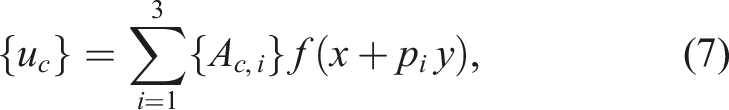
By utilization of the fundamental equations, an equation of sixth order with the unknown roots p _i (i = 1, 2, 3) is obtained. These roots are necessarily complex, which was proven by Eshelby et al., ²⁸ and correspond to the eigenvalues of the continuum. ²⁶ Based on the fact, that the coefficients are real and elastic stability must be met, these solutions appear in three complex conjugate pairs. ²⁹ For the real displacements all imaginary parts vanish and only the real parts have to be considered. ²⁸ For the respective continuum and load case simplifications can be made and the particular solutions are found through boundary conditions. The general solution can be superposed from the particular solutions.

Comparison of Lekhnitskii and Stroh

For a long time it was only assumed that both formulations are equivalent regarding their sextic equations. It was finally proven by Barnett and Kirchner ²⁹ by reducing the six-dimensional formulation of Stroh into two homogeneous, linear algebraic equations in terms of the reduced compliances. A more direct comparison of the coefficents, depending on the formulation as functions of the stiffnesses or reduced compliances, isn’t possible. According to Tarn and Wang, ³⁰ the Lekhnitskii-formulation facilitates the representation of the stresses and the Stroh-formulation those of the displacements. Furthermore, the approach of Lekhnitskii ² is not feasible for static motions like the determination of eigenvalues and eigenforms. ³¹ Stroh ²⁶ enables this by reducing the deformation problem to the determination of the eigenvalues and eigenvectors of the system and connecting them to the constitutive law through special eigenrelations. ³² Barnett and Kirchner ²⁹ favorate the formulation of Stroh, ²⁶ because of a more direct computation and the already met compatibility conditions. But they also point out that the choice must be made in regards to the specific case.

General formulation of state-space approach

In addition to these two formulations, a mixed approach known as state-space approach exists, where the governing equations are derived from the fundamental equations in terms of stresses and displacements. This so-called state equation in general form is expressed by the derivation of a state vector {R}, usually consisting of three displacements and three selected stresses. For most models the stresses in radial direction are chosen and the state equation is

$\frac{\partial }{\partial r}\left\{R\right\}=\left[A\left(r\right)\right]\hspace{0.17em}\left\{R\right\}.$

(8)

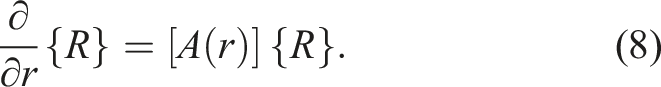
A second equation {S} = [B(r)] {R} is used after solving the state equation for the computation of the vector {S}, containing the remaining three stress components. Matrices [A(r)] and [B(r)] are linear differential operators, which depend on one coordinate, here r, but only consist of derivations of the other two coordinates. ³³ Although state-space models use elastic equations in three-dimensional form, they must discretize in at least one coordinate direction for a unique solution because of the fact that, for the usual boundary conditions, the state equation becomes a partial differential equation with infinite order. ³³ As a rule, an approximation method by node subdivision is applied, for example, by means of the finite-difference method, the finite-element method or a series development in the laminate plane (here z-θ). In this way, the state equation is converted into a system of linear differential equations that can be solved using standard methods by integrating the boundary conditions into the matrices [A(r)] and [B(r)]. However, the boundary conditions at the end faces of the continuum must again be formulated by simplifications in certain coordinate directions. Exact solutions using three-dimensional elastic equations are only possible in special cases like Rogers et al. ³⁴ Therefore, most models in the state-space only deal with axisymmetric loads and, like the previous approaches, only allow changes of the displacements, strains and stresses in two coordinate directions.

Stress-Based approaches

In addition to the basic formulation of three-dimensional anisotropic elasticity, Lekhnitskii deals in his books ‘Theory of Elasticity of an Anisotropic Elastic Body’, ² and ‘Anisotropic Plates’ ³⁵ as well as numerous publications^36–38 with tasks regarding infinite plates, bars, beams, cylinders, pipes, and plates with elliptical defects or inclusions under differing axisymmetric or bending loads. Each further described literature is based on these formulations.

General formulation of the tube according to Lekhnitskii

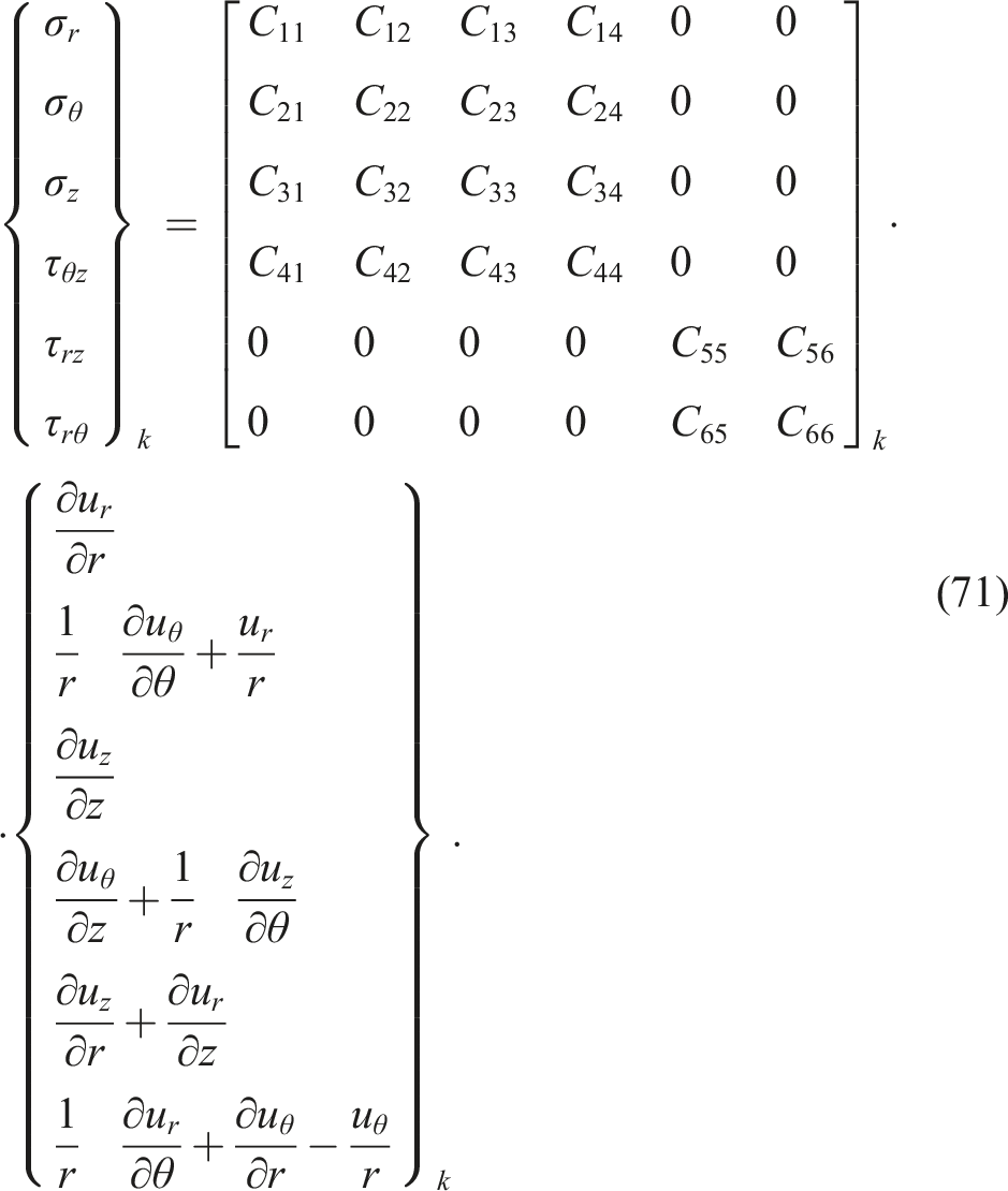
For the single-layered cylindrical tube, the fully populated constitutive law, corresponding to equation (1), is used initially. The tube is in the state of generalized plane strain, which means that a strain ɛ _z is present. However, like all other strains, displacements and stresses, it does not alter along the axial component. This allows a simplification of the contitutive law by a linear approach for the axial strain with

$\begin{array}{l}{\epsilon }_z=S_{33}\hspace{0.17em}\left(A\hspace{0.17em}x+B\hspace{0.17em}y+C\right)\\ =S_{33}\hspace{0.17em}\left(A\hspace{0.17em}r\hspace{0.17em}\sin \hspace{0.17em}\theta +B\hspace{0.17em}r\hspace{0.17em}\cos \hspace{0.17em}\theta +C\right).\end{array}$

(9)

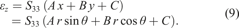
It is assumed that the axial strain only results from the axial stress σ _z and consists of one component for each of the bending moments about the x- and y-axis as well as one component for the axisymmetric loads. The unknowns A, B, and C represent the magnitudes of these stresses that increase with distance x or y to the neutral fiber for a moment load (A and B) and are constant for an axial load (C). By substituting the equation (9) into the third equation of (1), the stress in z direction can be computed and inserted into the remaining equations of (1). The result is the reduced material law

$\begin{array}{l}{\epsilon }_r={\beta }_{11}\hspace{0.17em}{\sigma }_r+{\beta }_{12}\hspace{0.17em}{\sigma }_{\theta }+{\beta }_{14}\hspace{0.17em}{\tau }_{\theta z}+{\beta }_{15}\hspace{0.17em}{\tau }_{rz}+{\beta }_{16}\hspace{0.17em}{\tau }_{r\theta }\\ +S_{33}\hspace{0.17em}\left(A\hspace{0.17em}r\hspace{0.17em}\sin \hspace{0.17em}\theta +B\hspace{0.17em}r\hspace{0.17em}\cos \hspace{0.17em}\theta +C\right),\\ {\epsilon }_{\theta }={\beta }_{21}\hspace{0.17em}{\sigma }_r+{\beta }_{22}\hspace{0.17em}{\sigma }_{\theta }+{\beta }_{24}\hspace{0.17em}{\tau }_{\theta z}+{\beta }_{25}\hspace{0.17em}{\tau }_{rz}+{\beta }_{26}\hspace{0.17em}{\tau }_{r\theta }\\ +S_{33}\hspace{0.17em}\left(A\hspace{0.17em}r\hspace{0.17em}\sin \hspace{0.17em}\theta +B\hspace{0.17em}r\hspace{0.17em}\cos \hspace{0.17em}\theta +C\right),\\ {\gamma }_{\theta z}={\beta }_{41}\hspace{0.17em}{\sigma }_r+{\beta }_{42}\hspace{0.17em}{\sigma }_{\theta }+{\beta }_{44}\hspace{0.17em}{\tau }_{\theta z}+{\beta }_{45}\hspace{0.17em}{\tau }_{rz}+{\beta }_{46}\hspace{0.17em}{\tau }_{r\theta }\\ +S_{33}\hspace{0.17em}\left(A\hspace{0.17em}r\hspace{0.17em}\sin \hspace{0.17em}\theta +B\hspace{0.17em}r\hspace{0.17em}\cos \hspace{0.17em}\theta +C\right),\\ {\gamma }_{rz}={\beta }_{51}\hspace{0.17em}{\sigma }_r+{\beta }_{52}\hspace{0.17em}{\sigma }_{\theta }+{\beta }_{54}\hspace{0.17em}{\tau }_{\theta z}+{\beta }_{55}\hspace{0.17em}{\tau }_{rz}+{\beta }_{56}\hspace{0.17em}{\tau }_{r\theta }\\ +S_{33}\hspace{0.17em}\left(A\hspace{0.17em}r\hspace{0.17em}\sin \hspace{0.17em}\theta +B\hspace{0.17em}r\hspace{0.17em}\cos \hspace{0.17em}\theta +C\right),\\ {\gamma }_{r\theta }={\beta }_{61}\hspace{0.17em}{\sigma }_r+{\beta }_{62}\hspace{0.17em}{\sigma }_{\theta }+{\beta }_{64}\hspace{0.17em}{\tau }_{\theta z}+{\beta }_{65}\hspace{0.17em}{\tau }_{rz}+{\beta }_{66}\hspace{0.17em}{\tau }_{r\theta }\\ +S_{33}\hspace{0.17em}\left(A\hspace{0.17em}r\hspace{0.17em}\sin \hspace{0.17em}\theta +B\hspace{0.17em}r\hspace{0.17em}\cos \hspace{0.17em}\theta +C\right),\end{array}$

(10)

with the reduced compliances

${\beta }_{ij}=S_{ij}-\frac{S_{i3}\hspace{1em}{S}_{3j}}{S_{33}}\text{for}i,j=\mathrm{1,2,4,5,6}.$

(11)

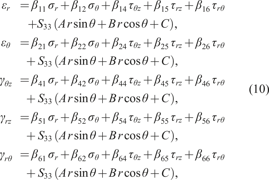
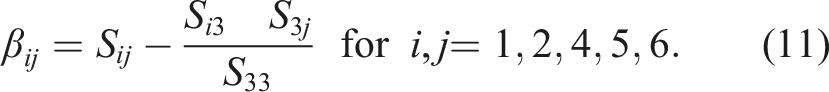
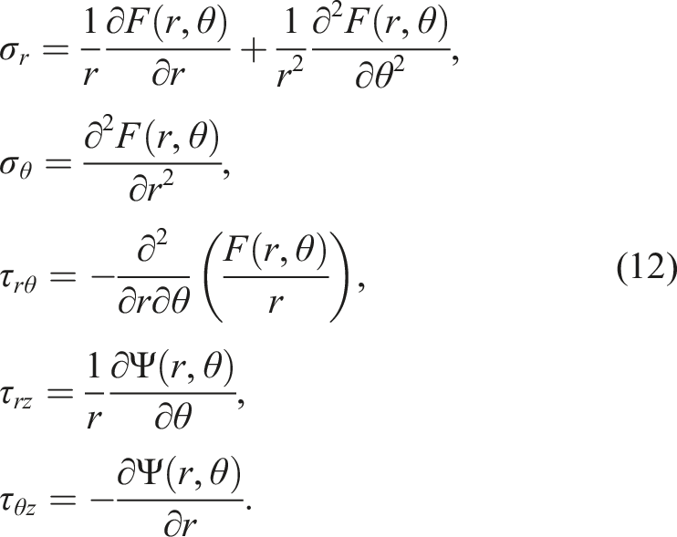
Furthermore an approach according to the stress functions of Airy F(r, θ) and Prandtl Ψ(r, θ) for the remaining five stresses is used. These stress functions meet the given equilibrium equation (5) and allow the boundary value problem to be converted to only two stress variables. Stresses can then be written as

$\begin{array}{l}{\sigma }_r=\frac{1}{r}\hspace{0.17em}\frac{\partial F\left(r,\theta \right)}{\partial r}+\frac{1}{r^2}\hspace{0.17em}\frac{{\partial }^{2}F\left(r,\theta \right)}{\partial {\theta }^2},\\ {\sigma }_{\theta }=\frac{{\partial }^{2}F\left(r,\theta \right)}{\partial r^2},\\ {\tau }_{r\theta }=-\frac{{\partial }^2}{\partial r\partial \theta }\hspace{0.17em}\left(\frac{F\left(r,\theta \right)}{r}\right),\\ {\tau }_{rz}=\frac{1}{r}\hspace{0.17em}\frac{\partial \mathrm{\Psi }\left(r,\theta \right)}{\partial \theta },\\ {\tau }_{\theta z}=-\frac{\partial \mathrm{\Psi }\left(r,\theta \right)}{\partial r}.\end{array}$

(12)

The six strains are described by only three displacements in the strain-displacement relations (6), which implies that they can’t be independent of one another and must meet compatibility requirements. The equation (6) are therefore inserted into the material law (2). By integration of the 3rd, 4th and 5th equation of the resulting system over the z-axis and conversion to the displacements, the following equations can be deduced

$\begin{array}{l}{u}_z=z\hspace{0.17em}\left(S_{31}\hspace{0.17em}{\sigma }_r+S_{32}\hspace{0.17em}{\sigma }_{\theta }+S_{33}\hspace{0.17em}{\sigma }_z+S_{34}\hspace{0.17em}{\tau }_{\theta z}+S_{35}\hspace{0.17em}{\tau }_{rz}+S_{36}\hspace{0.17em}{\tau }_{r\theta }\right)\\ +U_{z,0}\left(r,\theta \right),\\ u_{\theta }=z\hspace{0.17em}\left(S_{41}\hspace{0.17em}{\sigma }_r+S_{42}\hspace{0.17em}{\sigma }_{\theta }+S_{43}\hspace{0.17em}{\sigma }_z+S_{44}\hspace{0.17em}{\tau }_{\theta z}+S_{45}\hspace{0.17em}{\tau }_{rz}+S_{46}\hspace{0.17em}{\tau }_{r\theta }\right)\\ -\frac{z^2}{2}\hspace{0.17em}\frac{1}{r}\hspace{0.17em}\frac{\partial \left(S_{31}\hspace{0.17em}{\sigma }_r+S_{32}\hspace{0.17em}{\sigma }_{\theta }+S_{33}\hspace{0.17em}{\sigma }_z+S_{34}\hspace{0.17em}{\tau }_{\theta z}+S_{35}\hspace{0.17em}{\tau }_{rz}+S_{36}\hspace{0.17em}{\tau }_{r\theta }\right)}{\partial \theta }\\ -\frac{z}{r}\hspace{0.17em}\frac{\partial U_{z,0}}{\partial \theta }+U_{\theta ,0}\left(r,\theta \right),\\ u_r=z\hspace{0.17em}\left(S_{51}\hspace{0.17em}{\sigma }_r+S_{52}\hspace{0.17em}{\sigma }_{\theta }+S_{53}\hspace{0.17em}{\sigma }_z+S_{54}\hspace{0.17em}{\tau }_{\theta z}+S_{55}\hspace{0.17em}{\tau }_{rz}+S_{56}\hspace{0.17em}{\tau }_{r\theta }\right)\\ -\frac{z^2}{2}\hspace{0.17em}\frac{\partial \left(S_{31}\hspace{0.17em}{\sigma }_r+S_{32}\hspace{0.17em}{\sigma }_{\theta }+S_{33}\hspace{0.17em}{\sigma }_z+S_{34}\hspace{0.17em}{\tau }_{\theta z}+S_{35}\hspace{0.17em}{\tau }_{rz}+S_{36}\hspace{0.17em}{\tau }_{r\theta }\right)}{\partial r}\\ -z\frac{\partial U_{z,0}}{\partial r}+U_{r,0}\left(r,\theta \right).\end{array}$

(13)

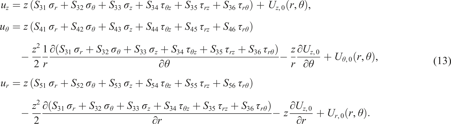
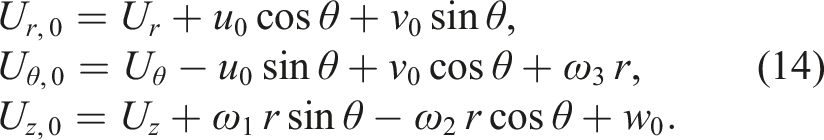
By using the displacements due to strains U _r , U _θ , U _z in the cylindrical coordinate system as well as the translatory u₀, v₀, w₀ and rotatory ω₁, ω₂, ω₃ rigid-body motions in the cartesian coordinate system, equations for the unknown displacement functions, resulting from the integration, can be established. Due to the small angles, the rigid-body motions can be transformed into the cylindrical system by means of the trigonometric functions. The displacement field is thus given by Lekhnitskii ² in the form

$\begin{array}{l}{U}_{r,0}=U_r+u_0\hspace{0.17em}\cos \hspace{0.17em}\theta +v_0\hspace{0.17em}\sin \hspace{0.17em}\theta ,\\ U_{\theta ,0}=U_{\theta }-u_0\hspace{0.17em}\sin \hspace{0.17em}\theta +v_0\hspace{0.17em}\cos \hspace{0.17em}\theta +{\omega }_3\hspace{0.17em}r,\\ U_{z,0}=U_z+{\omega }_1\hspace{0.17em}r\hspace{0.17em}\sin \hspace{0.17em}\theta -{\omega }_2\hspace{0.17em}r\hspace{0.17em}\cos \hspace{0.17em}\theta +w_0.\end{array}$

(14)

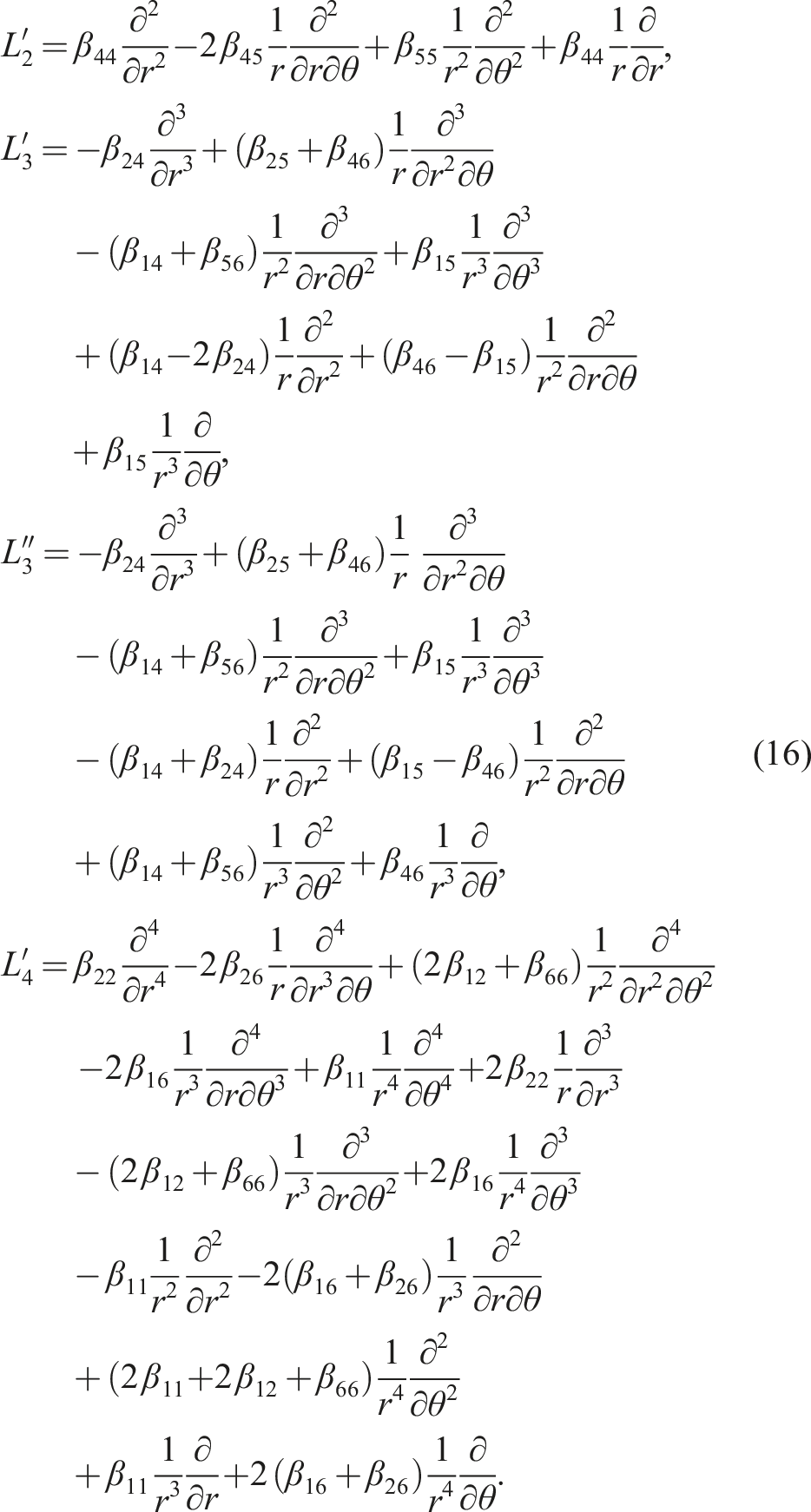
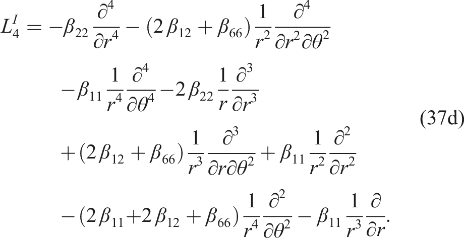
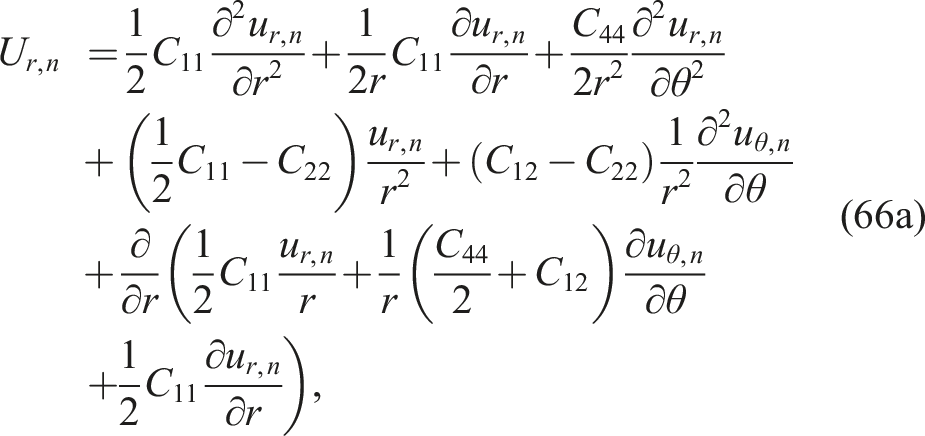
For compatibility, the equation (13) must be substituted into the other three equations of the constitutive law (2). The governing partial differential equation system can be established as a function of stress functions using the reduced constitutive law (10), the stress function approach (12), the displacements (13) and the displacements resulting from integration and expressed by the displacement field (14). For brevity, the system results in ²

$\begin{array}{l}{L}_4^{\prime }\hspace{0.17em}F+L_3^{\prime }\hspace{0.17em}\mathrm{\Psi }=2\hspace{0.17em}\left[\left(S_{13}-S_{23}\right)\hspace{0.17em}A-S_{36}\hspace{0.17em}B\right]\hspace{0.17em}\frac{\sin \hspace{0.17em}\theta }{r}\\ \hspace{1em}\hspace{1em}\hspace{1em}\hspace{1em}\hspace{1em}\hspace{1em}\hspace{1em}\hspace{1em}\hspace{1em}+2\hspace{0.17em}\left[S_{36}\hspace{0.17em}A+\left(S_{13}-S_{23}\right)\hspace{0.17em}B\right]\hspace{0.17em}\frac{\cos \hspace{0.17em}\theta }{r},\end{array}$

(15a)

$\begin{array}{l}{L}_3^{″}\hspace{0.17em}F+L_2^{\prime }\hspace{0.17em}\mathrm{\Psi }=\left(-S_{35}\hspace{0.17em}A+2\hspace{0.17em}{S}_{34}\hspace{0.17em}B\right)\hspace{0.17em}\cos \hspace{0.17em}\theta \\ \hspace{1em}\hspace{1em}\hspace{1em}\hspace{1em}\hspace{1em}\hspace{1em}\hspace{1em}\hspace{1em}\hspace{1em}+\left(2\hspace{0.17em}{S}_{34}\hspace{0.17em}A+S_{35}\hspace{0.17em}B\right)\hspace{0.17em}\sin \hspace{0.17em}\theta +C\hspace{0.17em}{S}_{34}\hspace{0.17em}\frac{1}{r}\end{array}.$

(15b)

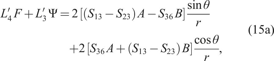
The differential operators of second order $L_2^{\prime }$ , third order $L_3^{\prime }$ , $L_3^{″}$ and fourth order $L_4^{\prime }$ are

$\begin{array}{l}{L}_2^{\prime }={\beta }_{44}\hspace{0.17em}\frac{{\partial }^2}{\partial r^2}-2\hspace{0.17em}{\beta }_{45}\hspace{0.17em}\frac{1}{r}\hspace{0.17em}\frac{{\partial }^2}{\partial r\partial \theta }+{\beta }_{55}\hspace{0.17em}\frac{1}{r^2}\hspace{0.17em}\frac{{\partial }^2}{\partial {\theta }^2}+{\beta }_{44}\hspace{0.17em}\frac{1}{r}\hspace{0.17em}\frac{\partial }{\partial r},\\ L_3^{\prime }=-{\beta }_{24}\hspace{0.17em}\frac{{\partial }^3}{\partial r^3}+\left({\beta }_{25}+{\beta }_{46}\right)\hspace{0.17em}\frac{1}{r}\hspace{0.17em}\frac{{\partial }^3}{\partial r^2\partial \theta }\\ -\left({\beta }_{14}+{\beta }_{56}\right)\hspace{0.17em}\frac{1}{r^2}\hspace{0.17em}\frac{{\partial }^3}{\partial r\partial {\theta }^2}+{\beta }_{15}\hspace{0.17em}\frac{1}{r^3}\hspace{0.17em}\frac{{\partial }^3}{\partial {\theta }^3}\\ +\left({\beta }_{14}-2\hspace{0.17em}{\beta }_{24}\right)\hspace{0.17em}\frac{1}{r}\hspace{0.17em}\frac{{\partial }^2}{\partial r^2}+\left({\beta }_{46}-{\beta }_{15}\right)\hspace{0.17em}\frac{1}{r^2}\hspace{0.17em}\frac{{\partial }^2}{\partial r\partial \theta }\\ +{\beta }_{15}\hspace{0.17em}\frac{1}{r^3}\hspace{0.17em}\frac{\partial }{\partial \theta },\\ L_3^{″}=-{\beta }_{24}\hspace{0.17em}\frac{{\partial }^3}{\partial r^3}+\left({\beta }_{25}+{\beta }_{46}\right)\hspace{0.17em}\frac{1}{r}\hspace{1em}\frac{{\partial }^3}{\partial r^2\partial \theta }\\ -\left({\beta }_{14}+{\beta }_{56}\right)\hspace{0.17em}\frac{1}{r^2}\hspace{0.17em}\frac{{\partial }^3}{\partial r\partial {\theta }^2}+{\beta }_{15}\hspace{0.17em}\frac{1}{r^3}\hspace{0.17em}\frac{{\partial }^3}{\partial {\theta }^3}\\ -\left({\beta }_{14}+{\beta }_{24}\right)\hspace{0.17em}\frac{1}{r}\hspace{0.17em}\frac{{\partial }^2}{\partial r^2}+\left({\beta }_{15}-{\beta }_{46}\right)\hspace{0.17em}\frac{1}{r^2}\hspace{0.17em}\frac{{\partial }^2}{\partial r\partial \theta }\\ +\left({\beta }_{14}+{\beta }_{56}\right)\hspace{0.17em}\frac{1}{r^3}\hspace{0.17em}\frac{{\partial }^2}{\partial {\theta }^2}+{\beta }_{46}\hspace{0.17em}\frac{1}{r^3}\hspace{0.17em}\frac{\partial }{\partial \theta },\\ L_4^{\prime }={\beta }_{22}\hspace{0.17em}\frac{{\partial }^4}{\partial r^4}-2\hspace{0.17em}{\beta }_{26}\hspace{0.17em}\frac{1}{r}\hspace{0.17em}\frac{{\partial }^4}{\partial r^3\partial \theta }+\left(2\hspace{0.17em}{\beta }_{12}+{\beta }_{66}\right)\hspace{0.17em}\frac{1}{r^2}\hspace{0.17em}\frac{{\partial }^4}{\partial r^2\partial {\theta }^2}\\ -2\hspace{0.17em}{\beta }_{16}\hspace{0.17em}\frac{1}{r^3}\hspace{0.17em}\frac{{\partial }^4}{\partial r\partial {\theta }^3}+{\beta }_{11}\hspace{0.17em}\frac{1}{r^4}\hspace{0.17em}\frac{{\partial }^4}{\partial {\theta }^4}+2\hspace{0.17em}{\beta }_{22}\hspace{0.17em}\frac{1}{r}\hspace{0.17em}\frac{{\partial }^3}{\partial r^3}\\ -\left(2\hspace{0.17em}{\beta }_{12}+{\beta }_{66}\right)\hspace{0.17em}\frac{1}{r^3}\hspace{0.17em}\frac{{\partial }^3}{\partial r\partial {\theta }^2}+2\hspace{0.17em}{\beta }_{16}\hspace{0.17em}\frac{1}{r^4}\hspace{0.17em}\frac{{\partial }^3}{\partial {\theta }^3}\\ -{\beta }_{11}\frac{1}{r^2}\frac{{\partial }^2}{\partial r^2}-2\left({\beta }_{16}+{\beta }_{26}\right)\frac{1}{r^3}\frac{{\partial }^2}{\partial r\partial \theta }\\ +\left(2\hspace{0.17em}{\beta }_{11}+2\hspace{0.17em}{\beta }_{12}+{\beta }_{66}\right)\hspace{0.17em}\frac{1}{r^4}\hspace{0.17em}\frac{{\partial }^2}{\partial {\theta }^2}\\ +{\beta }_{11}\hspace{0.17em}\frac{1}{r^3}\hspace{0.17em}\frac{\partial }{\partial r}+2\hspace{0.17em}\left({\beta }_{16}+{\beta }_{26}\right)\hspace{0.17em}\frac{1}{r^4}\hspace{0.17em}\frac{\partial }{\partial \theta }.\end{array}$

(16)

Pure bending of the tube according to Lekhnitskii

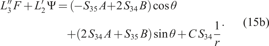
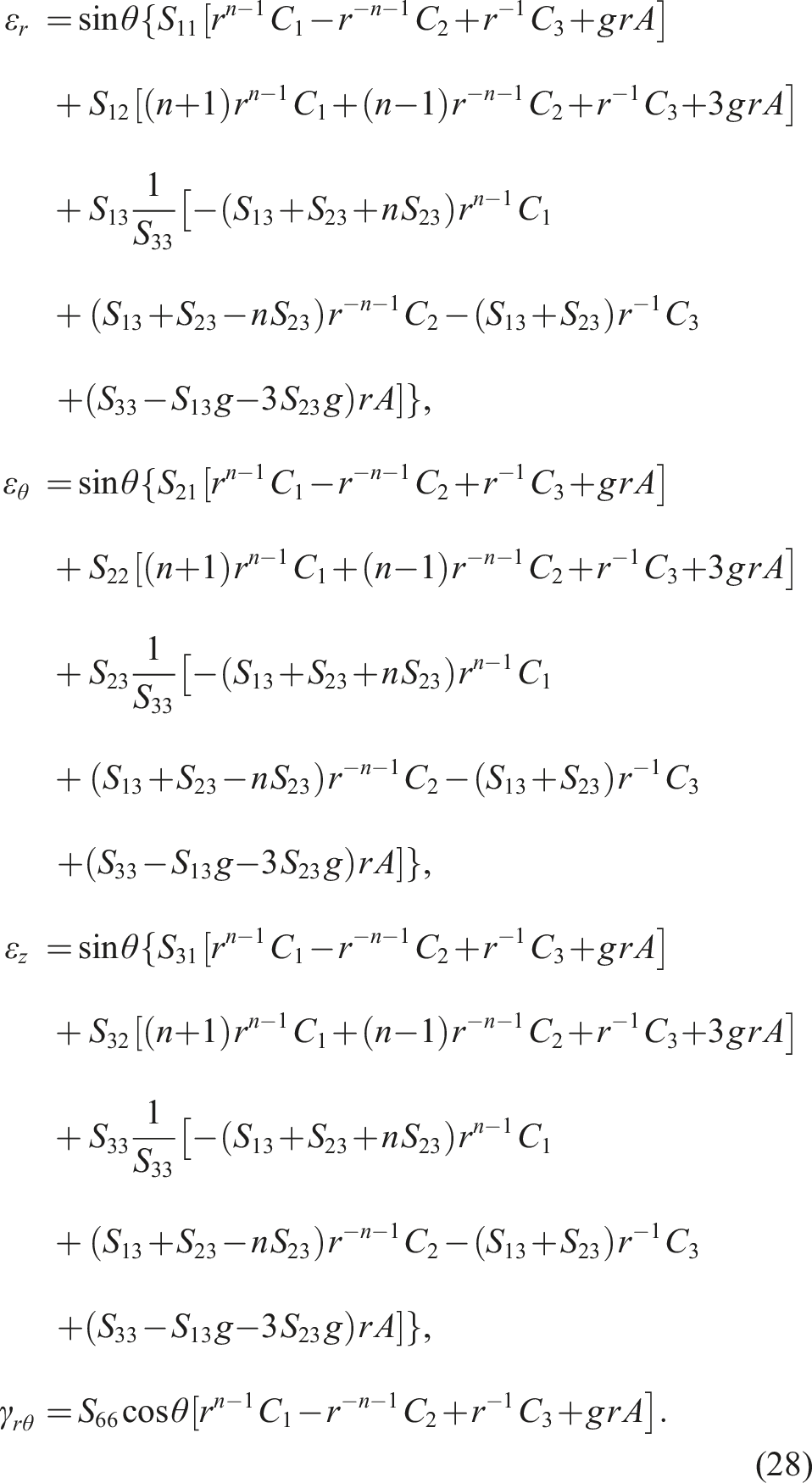
For the load case of pure bending around the y-axis, some simplifications can be made. The orthotropic constitutive law, see (4), is used and the following variables are set equal to zero

$\frac{\partial }{\partial z}=0;B=C=0;\mathrm{\Psi }=0.$

(17)

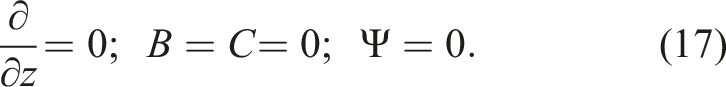
B and C as described in section General formulation of the tube according to Lekhnitskii are coupled to bending around the x-axis and axisymmetric loads. The Prandtl stress function Ψ is only considered for the load case of torsion. This simplifies the equation system (15a), simultaneously eliminating (15b), to

$\begin{array}{ll}& {\beta }_{22}\hspace{0.17em}\frac{{\partial }^{4}F}{\partial r^4}+\left(2\hspace{0.17em}{\beta }_{12}+{\beta }_{66}\right)\hspace{0.17em}\frac{1}{r^2}\hspace{0.17em}\frac{{\partial }^{4}F}{\partial r^2\partial {\theta }^2}+{\beta }_{11}\hspace{0.17em}\frac{1}{r^4}\hspace{0.17em}\frac{{\partial }^{4}F}{\partial {\theta }^4}\\ & +2\hspace{0.17em}{\beta }_{22}\hspace{0.17em}\frac{1}{r}\hspace{0.17em}\frac{{\partial }^{3}F}{\partial r^3}-\left(2\hspace{0.17em}{\beta }_{12}+{\beta }_{66}\right)\hspace{0.17em}\frac{1}{r^3}\hspace{0.17em}\frac{{\partial }^{3}F}{\partial r\partial {\theta }^2}\\ & -{\beta }_{11}\hspace{0.17em}\frac{1}{r^2}\hspace{0.17em}\frac{{\partial }^{2}F}{\partial r^2}+\left(2\hspace{0.17em}{\beta }_{11}+2\hspace{0.17em}{\beta }_{12}+{\beta }_{66}\right)\hspace{0.17em}\frac{1}{r^4}\hspace{0.17em}\frac{{\partial }^{2}F}{\partial {\theta }^2}\\ & +{\beta }_{11}\hspace{0.17em}\frac{1}{r^3}\hspace{0.17em}\frac{\partial F}{\partial r}=2\hspace{0.17em}\left(S_{13}-S_{23}\right)\hspace{0.17em}A\hspace{0.17em}\frac{\sin \hspace{0.17em}\theta }{r}.\end{array}$

(18)

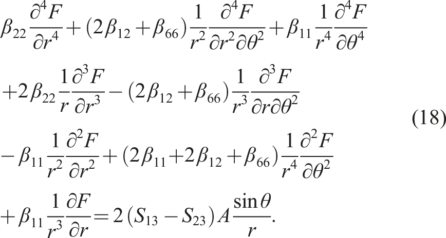
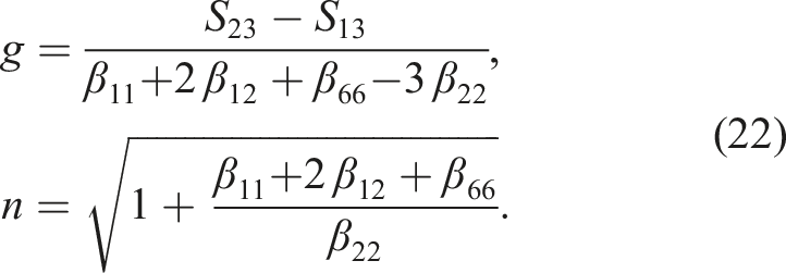
A solution for this partial differential system is searched, using a trigonometric approach in the form

$F=f\left(r\right)\hspace{0.17em}\sin \hspace{0.17em}\theta$

(19)

and results in a polynomial function of the fourth class with five unknowns C₁-C₄ and A by searching solutions for f(r) ²

$F=\left(\frac{C_1}{n}\hspace{0.17em}{r}^{1+n}+\frac{C_2}{n}\hspace{0.17em}{r}^{1-n}+C_3\hspace{0.17em}r\hspace{0.17em}\ln \hspace{0.17em}r+C_4\hspace{0.17em}r+A\hspace{0.17em}\frac{g}{2}\hspace{0.17em}{r}^3\right)\hspace{0.17em}\sin \hspace{0.17em}\theta .$

(20)

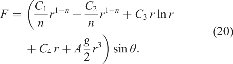
Substituting Equations (20) and (17) into (12) provides the stress distributions

$\begin{array}{ll}{\sigma }_r=& \left[C_1\hspace{0.17em}{r}^{\left(n-1\right)}-C_2\hspace{0.17em}{r}^{\left(-n-1\right)}+\frac{C_3}{r}+A\hspace{0.17em}g\hspace{0.17em}r\right]\cdot \hspace{0.17em}\sin \hspace{0.17em}\theta ,\\ {\sigma }_{\theta }=& \left[C_1\hspace{0.17em}\left(n+1\right)\hspace{0.17em}{r}^{n-1}+C_2\hspace{0.17em}\left(n-1\right)\hspace{0.17em}{r}^{-n-1}+\frac{C_3}{r}+3\hspace{0.17em}A\hspace{0.17em}g\hspace{0.17em}r\right]\\ & \cdot \hspace{0.17em}\sin \hspace{0.17em}\theta ,\\ {\sigma }_z=& A\hspace{0.17em}r\hspace{0.17em}\sin \hspace{0.17em}\theta -\frac{1}{S_{33}}\hspace{0.17em}\left(S_{13}\hspace{0.17em}{\sigma }_r+S_{23}\hspace{0.17em}{\sigma }_{\theta }\right),\\ {\tau }_{r\theta }=& -\left[C_1\hspace{0.17em}{r}^{n-1}-C_2\hspace{0.17em}{r}^{-n-1}+\frac{C_3}{r}+A\hspace{0.17em}g\hspace{0.17em}r\right]\hspace{0.17em}\cdot \cos \hspace{0.17em}\theta ,\end{array}$

(21)

with

$\begin{array}{l}g=\frac{S_{23}-S_{13}}{{\beta }_{11}+2\hspace{0.17em}{\beta }_{12}+{\beta }_{66}-3\hspace{0.17em}{\beta }_{22}},\\ n=\sqrt{1+\frac{{\beta }_{11}+2\hspace{0.17em}{\beta }_{12}+{\beta }_{66}}{{\beta }_{22}}}.\end{array}$

(22)

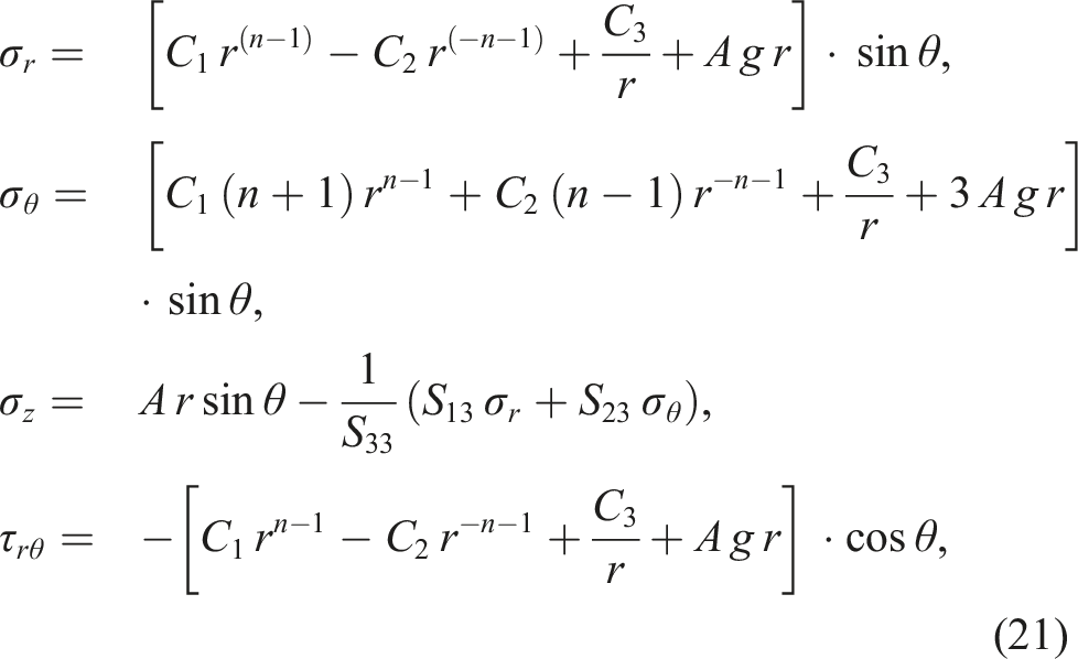
The unknowns C₁-C₃ and A must be found by the use of boundary conditions. Strains and displacements can be calculated utilizing the constitutive law (2) and the strain-displacement relations (6).

Multi-Layered tube according to Xia et al

Composites represent a multi-layer design with different fiber angles and thus local coordinate systems for each layer. Therefore, the Lekhnitskii tube model is used for each individual layer and solved with continuity conditions on the interphases for enhancements like the model by Xia et al. ³⁹

Transformation and simplification of a single layer

The compliances of each layer must be transformed from the local (1, 2, 3) into the global coordinate system (r, θ, z) around the related fiber angle α, see Figure 1.

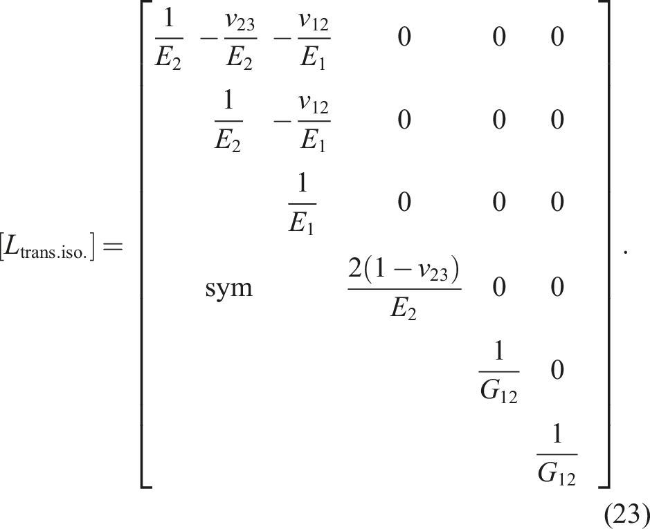
The local compliances are indicated by [L _ij ] (i, j = 1-6) in transversely isotropic form in accordance with equation (4). The engineering constants can be used to express the compliances of a unidirectional layer as

$\left[L_{\text{trans}.\text{iso}.}\right]=\left[\begin{array}{cccccc}\frac{1}{E_2}& -\frac{{\nu }_{23}}{E_2}& -\frac{{\nu }_{12}}{E_1}& 0& 0& 0\\ & \frac{1}{E_2}& -\frac{{\nu }_{12}}{E_1}& 0& 0& 0\\ & & \frac{1}{E_1}& 0& 0& 0\\ & \text{sym}& & \frac{2\left(1-{\nu }_{23}\right)}{E_2}& 0& 0& \\ & & & & \frac{1}{G_{12}}& 0\\ & & & & & \frac{1}{G_{12}}\end{array}\right].$

(23)

However, it should be noted that the local constituitve law is formulated by Xia et al. ³⁹ using the permutated notation ${\left\{{\sigma }_3,{\sigma }_2,{\sigma }_1,{\tau }_{23},{\tau }_{12},{\tau }_{13}\right\}}^T$ instead of the common notation ${\left\{{\sigma }_1,{\sigma }_2,{\sigma }_3,{\tau }_{23},{\tau }_{13},{\tau }_{12}\right\}}^T$ used for example in laminate theories. This also changes the positions of the individual entries in the stiffness and compliance matrix. Transverse isotropy implies that E₃ = E₂, ν₁₃ = ν₁₂ and G₁₃ = G₁₂. Further details on the necessity of transforming the material properties for application to bending models and another possibility of permutation can be found in Siegl and Ehrlich. ³ The global constitutive law of each layer can be expressed by

$\left\{\begin{array}{l}{\epsilon }_r\\ {\epsilon }_{\theta }\\ {\epsilon }_z\\ {\gamma }_{r\theta }\\ {\gamma }_{\theta z}\\ {\gamma }_{zr}\end{array}\right\}={\left[Q_{ij}\right]}^{-1}\hspace{0.17em}\left[L_{ij}\right]\hspace{0.17em}\left[P_{ij}\right]\hspace{0.17em}\left\{\begin{array}{l}{\sigma }_r\\ {\sigma }_{\theta }\\ {\sigma }_z\\ {\tau }_{r\theta }\\ {\tau }_{\theta z}\\ {\tau }_{zr}\end{array}\right\}=\left[S_{ij}\right]\hspace{0.17em}\left\{\begin{array}{l}{\sigma }_r\\ {\sigma }_{\theta }\\ {\sigma }_z\\ {\tau }_{r\theta }\\ {\tau }_{\theta z}\\ {\tau }_{zr}\end{array}\right\}$

(24)

in which the transformation matrices are

$\left[Q_{ij}\right]=\left[\begin{array}{cccccc}1& 0& 0& 0& 0& 0\\ 0& c^2\alpha & s^2\alpha & 0& -c\alpha \hspace{0.17em}s\alpha & 0\\ 0& s^2\alpha & c^2\alpha & 0& c\alpha \hspace{0.17em}s\alpha & 0\\ 0& 0& 0& c\alpha & 0& -s\alpha \\ 0& 2\hspace{0.17em}c\alpha s\alpha & -2\hspace{0.17em}c\alpha s\alpha & 0& c^2\alpha -s^2\alpha & 0\\ 0& 0& 0& s\alpha & 0& c\alpha \end{array}\right]$

(25)

and

$\left[P_{ij}\right]=\left[\begin{array}{cccccc}1& 0& 0& 0& 0& 0\\ 0& c^2\alpha & s^2\alpha & 0& -2\hspace{0.17em}c\alpha \hspace{0.17em}s\alpha & 0\\ 0& s^2\alpha & c^2\alpha & 0& 2\hspace{0.17em}c\alpha \hspace{0.17em}s\alpha & 0\\ 0& 0& 0& c\alpha & 0& -s\alpha \\ 0& c\alpha \hspace{0.17em}s\alpha & -c\alpha \hspace{0.17em}s\alpha & 0& c^2\alpha -s^2\alpha & 0\\ 0& 0& 0& s\alpha & 0& c\alpha \end{array}\right]$

(26)

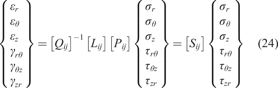
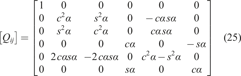
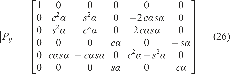
Trigonometric functions in (25) and (26) are abbreviated with c = cos and s = sin. The global constitutive law of each layer is further simplified by setting compliances S₁₆, S₂₆, S₃₆, S₄₄, S₅₅, S₆₁, S₆₂ and S₆₃ equal to zero. Coupling effects of a monotropic single layer and shear stresses τ _zr and τ _θz as well as transverse contraction effects are thus neglected. Note that Xia et al. ³⁹ also permuted the global constitutive law according to Lekhnitskii ² from ${\left\{{\sigma }_r,{\sigma }_{\theta },{\sigma }_z,{\tau }_{\theta z},{\tau }_{rz},{\tau }_{r\theta }\right\}}^T$ to ${\left\{{\sigma }_r,{\sigma }_{\theta },{\sigma }_z,{\tau }_{r\theta },{\tau }_{\theta z},{\tau }_{rz}\right\}}^T$ , which leads to the redefinition of S₆₆ to S₄₄ in the equation for γ _rθ . For consistency, the definition of Lekhnitskii ² is used and results in

$\begin{array}{l}{\epsilon }_r=S_{11}\hspace{0.17em}{\sigma }_r+S_{12}\hspace{0.17em}{\sigma }_{\theta }+S_{13}\hspace{0.17em}{\sigma }_z,\\ {\epsilon }_{\theta }=S_{21}\hspace{0.17em}{\sigma }_r+S_{22}\hspace{0.17em}{\sigma }_{\theta }+S_{23}\hspace{0.17em}{\sigma }_z,\\ {\epsilon }_z=S_{31}\hspace{0.17em}{\sigma }_r+S_{32}\hspace{0.17em}{\sigma }_{\theta }+S_{33}\hspace{0.17em}{\sigma }_z,\\ {\gamma }_{r\theta }=S_{66}\hspace{0.17em}{\tau }_{r\theta }.\end{array}$

(27)

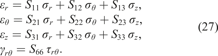
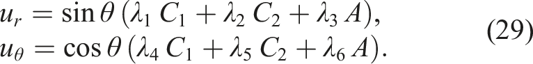
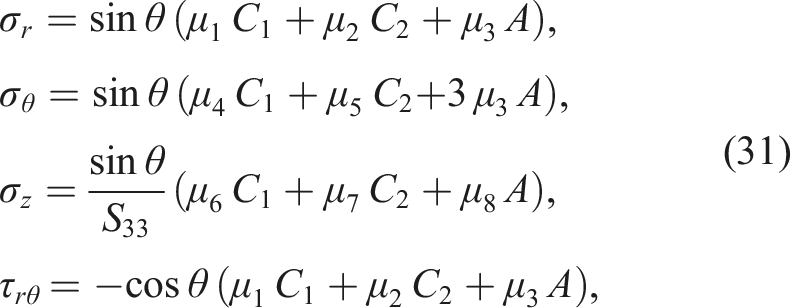
By substituting the stress distributions for a single layer under pure bending from equation (21) into the constitutive law (27), the equations for the strains are obtained by Pavlou ⁴⁰ with

$\begin{array}{l}{\epsilon }_r=\hspace{0.17em}\sin \hspace{0.17em}\theta \hspace{0.17em}\{S_{11}\hspace{0.17em}\left[r^{n-1}\hspace{0.17em}{C}_1-r^{-n-1}\hspace{0.17em}{C}_2+r^{-1}\hspace{0.17em}{C}_3+g\hspace{0.17em}r\hspace{0.17em}A\right]\\ +S_{12}\hspace{0.17em}\left[\left(n+1\right)\hspace{0.17em}{r}^{n-1}\hspace{0.17em}{C}_1+\left(n-1\right)\hspace{0.17em}{r}^{-n-1}\hspace{0.17em}{C}_2+r^{-1}\hspace{0.17em}{C}_3+3\hspace{0.17em}g\hspace{0.17em}r\hspace{0.17em}A\right]\\ +S_{13}\hspace{0.17em}\frac{1}{S_{33}}\hspace{0.17em}[-\left(S_{13}+S_{23}+n\hspace{0.17em}{S}_{23}\right)\hspace{0.17em}{r}^{n-1}\hspace{0.17em}{C}_1\\ +\left(S_{13}+S_{23}-n\hspace{0.17em}{S}_{23}\right)\hspace{0.17em}{r}^{-n-1}\hspace{0.17em}{C}_2-\left(S_{13}+S_{23}\right)\hspace{0.17em}{r}^{-1}\hspace{0.17em}{C}_3\\ +\left(S_{33}-S_{13}\hspace{0.17em}g-3\hspace{0.17em}{S}_{23}\hspace{0.17em}g\right)\hspace{0.17em}r\hspace{0.17em}A]\},\\ {\epsilon }_{\theta }=\hspace{0.17em}\sin \hspace{0.17em}\theta \hspace{0.17em}\{S_{21}\hspace{0.17em}\left[r^{n-1}\hspace{0.17em}{C}_1-r^{-n-1}\hspace{0.17em}{C}_2+r^{-1}\hspace{0.17em}{C}_3+g\hspace{0.17em}r\hspace{0.17em}A\right]\\ +S_{22}\hspace{0.17em}\left[\left(n+1\right)\hspace{0.17em}{r}^{n-1}\hspace{0.17em}{C}_1+\left(n-1\right)\hspace{0.17em}{r}^{-n-1}\hspace{0.17em}{C}_2+r^{-1}\hspace{0.17em}{C}_3+3\hspace{0.17em}g\hspace{0.17em}r\hspace{0.17em}A\right]\\ +S_{23}\hspace{0.17em}\frac{1}{S_{33}}\hspace{0.17em}[-\left(S_{13}+S_{23}+n\hspace{0.17em}{S}_{23}\right)\hspace{0.17em}{r}^{n-1}\hspace{0.17em}{C}_1\\ +\left(S_{13}+S_{23}-n\hspace{0.17em}{S}_{23}\right)\hspace{0.17em}{r}^{-n-1}\hspace{0.17em}{C}_2-\left(S_{13}+S_{23}\right)\hspace{0.17em}{r}^{-1}\hspace{0.17em}{C}_3\\ +\left(S_{33}-S_{13}\hspace{0.17em}g-3\hspace{0.17em}{S}_{23}\hspace{0.17em}g\right)\hspace{0.17em}r\hspace{0.17em}A]\},\\ {\epsilon }_z=\hspace{0.17em}\sin \hspace{0.17em}\theta \hspace{0.17em}\{S_{31}\hspace{0.17em}\left[r^{n-1}\hspace{0.17em}{C}_1-r^{-n-1}\hspace{0.17em}{C}_2+r^{-1}\hspace{0.17em}{C}_3+g\hspace{0.17em}r\hspace{0.17em}A\right]\\ +S_{32}\hspace{0.17em}\left[\left(n+1\right)\hspace{0.17em}{r}^{n-1}\hspace{0.17em}{C}_1+\left(n-1\right)\hspace{0.17em}{r}^{-n-1}\hspace{0.17em}{C}_2+r^{-1}\hspace{0.17em}{C}_3+3\hspace{0.17em}g\hspace{0.17em}r\hspace{0.17em}A\right]\\ +S_{33}\hspace{0.17em}\frac{1}{S_{33}}\hspace{0.17em}[-\left(S_{13}+S_{23}+n\hspace{0.17em}{S}_{23}\right)\hspace{0.17em}{r}^{n-1}\hspace{0.17em}{C}_1\\ +\left(S_{13}+S_{23}-n\hspace{0.17em}{S}_{23}\right)\hspace{0.17em}{r}^{-n-1}\hspace{0.17em}{C}_2-\left(S_{13}+S_{23}\right)\hspace{0.17em}{r}^{-1}\hspace{0.17em}{C}_3\\ +\left(S_{33}-S_{13}\hspace{0.17em}g-3\hspace{0.17em}{S}_{23}\hspace{0.17em}g\right)\hspace{0.17em}r\hspace{0.17em}A]\},\\ {\gamma }_{r\theta }=\hspace{0.17em}{S}_{66}\hspace{0.17em}\cos \hspace{0.17em}\theta \hspace{0.17em}\left[r^{n-1}\hspace{0.17em}{C}_1-r^{-n-1}\hspace{0.17em}{C}_2+r^{-1}\hspace{0.17em}{C}_3+g\hspace{0.17em}r\hspace{0.17em}A\right].\end{array}$

(28)

The constant C₃ is set equal to zero because of the fact that the displacements are single-valued functions .^2,39 Otherwise the system would give an infinite number of solutions for C₁-C₃. In Zhang and Hoa ⁴¹ it is assumed that Lekhnitskii ² found this solution empirically. By inserting the strains ɛ _r and ɛ _θ from (28) into the strain-displacement relations (6), integration and conversion, the displacements u _r and u _θ can be arranged to ⁴⁰

$\begin{array}{l}{u}_r=\sin \hspace{0.17em}\theta \hspace{0.17em}\left({\lambda }_1\hspace{0.17em}{C}_1+{\lambda }_2\hspace{0.17em}{C}_2+{\lambda }_3\hspace{0.17em}A\right),\\ u_{\theta }=\cos \hspace{0.17em}\theta \hspace{0.17em}\left({\lambda }_4\hspace{0.17em}{C}_1+{\lambda }_5\hspace{0.17em}{C}_2+{\lambda }_6\hspace{0.17em}A\right).\end{array}$

(29)

The abbreviations for the coefficents are

$\begin{array}{l}{\lambda }_1=-2\left[S_{13}^2+\left(n+1\right)S_{23}{S}_{13}-S_{33}\left(S_{12}+n{S}_{12}+S_{11}\right)\right]r^{2n}\\ \cdot \left(\frac{r^{-n}}{2n{S}_{33}}\right),\\ {\lambda }_2=2\left[-S_{13}^2+\left(n-1\right)S_{23}{S}_{13}+S_{33}\left(S_{12}-n{S}_{12}+S_{11}\right)\right]\\ \cdot \left(\frac{r^{-n}}{2n{S}_{33}}\right),\\ {\lambda }_3=n{r}^{n+2}\left[S_{33}{S}_{13}+g\left(-S_{13}\left(S_{13}+3S_{23}\right)+S_{33}\left(3S_{12}+S_{11}\right)\right)\right]\\ \cdot \left(\frac{r^{-n}}{2n{S}_{33}}\right),\\ {\lambda }_4=2r^{2n}[n^2\left(S_{23}^2-S_{33}{S}_{22}\right)-S_{13}\left(S_{13}+S_{23}\right)\\ +n\left(S_{23}\left(S_{13}+S_{23}\right)-S_{23}{S}_{13}-S_{33}\left(S_{22}+2S_{12}\right)\right)\\ +S_{33}\left(S_{12}+S_{11}\right)]\left(\frac{r^{-n}}{2n{S}_{33}}\right),\\ {\lambda }_5=2[n^2\left(S_{23}^2-S_{33}{S}_{22}\right)-S_{13}\left(S_{13}+S_{23}\right)\\ +n\left(-S_{23}\left(S_{13}+S_{23}\right)+S_{23}{S}_{13}+S_{33}{S}_{22}\right)\\ +S_{33}\left(S_{12}+S_{11}\right)]\left(\frac{r^{-n}}{2n{S}_{33}}\right),\\ {\lambda }_6=n{r}^{n+2}[S_{33}\left(S_{13}-2S_{23}\right)+g(\left(S_{13}+3S_{23}\right)\left(2S_{23}-S_{13}\right)\\ +S_{33}\left(-6S_{22}+S_{12}+S_{11}\right))]\left(\frac{r^{-n}}{2n{S}_{33}}\right).\end{array}$

(30)

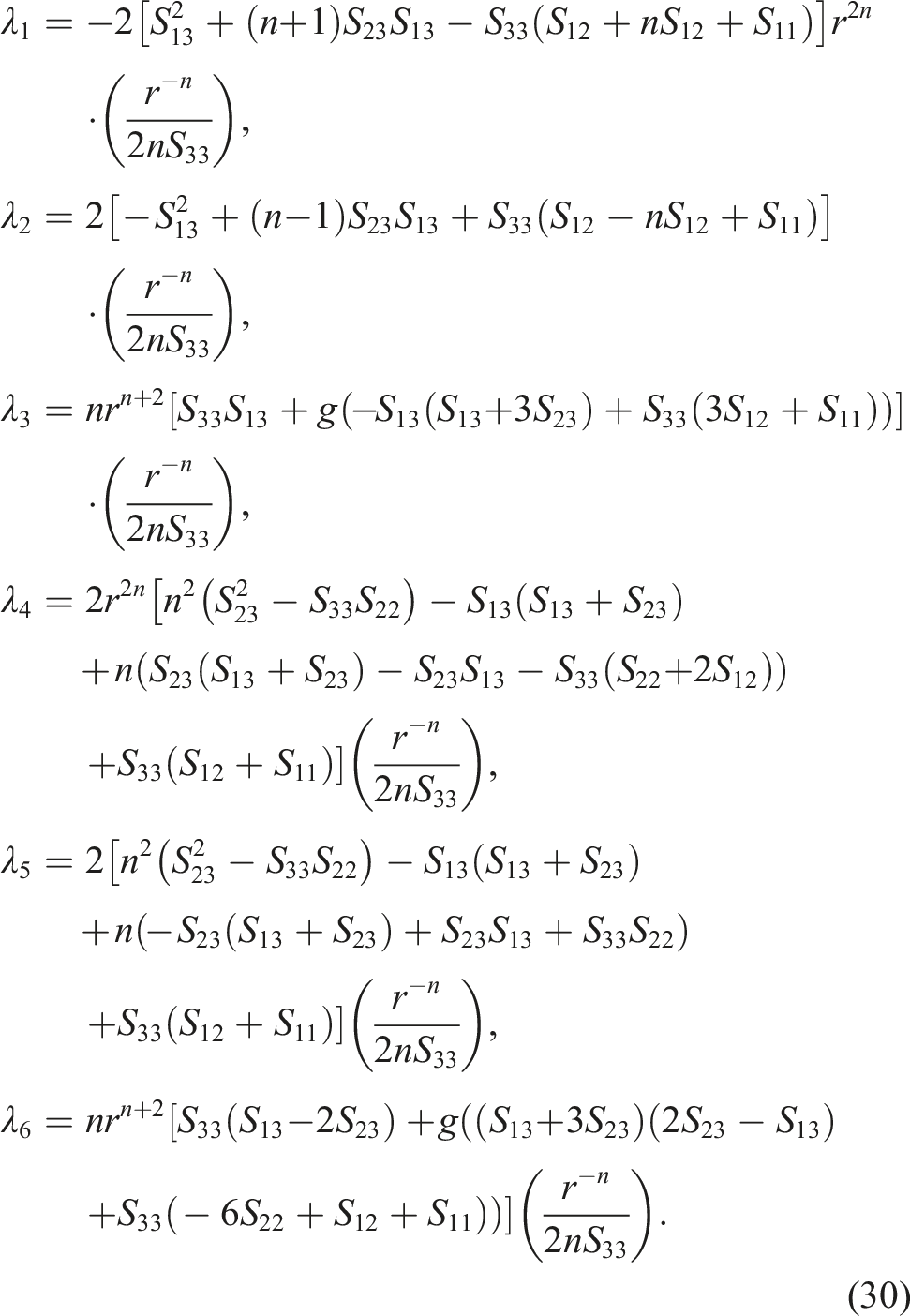
This rearrangement is also used for the stress distributions (21), which leads to

$\begin{array}{l}{\sigma }_r=\sin \hspace{0.17em}\theta \hspace{0.17em}\left({\mu }_1\hspace{0.17em}{C}_1+{\mu }_2\hspace{0.17em}{C}_2+{\mu }_3\hspace{0.17em}A\right),\\ {\sigma }_{\theta }=\sin \hspace{0.17em}\theta \hspace{0.17em}\left({\mu }_4\hspace{0.17em}{C}_1+{\mu }_5\hspace{0.17em}{C}_2+3\hspace{0.17em}{\mu }_3\hspace{0.17em}A\right),\\ {\sigma }_z=\frac{\sin \hspace{0.17em}\theta }{S_{33}}\hspace{0.17em}\left({\mu }_6\hspace{0.17em}{C}_1+{\mu }_7\hspace{0.17em}{C}_2+{\mu }_8\hspace{0.17em}A\right),\\ {\tau }_{r\theta }\hspace{0.17em}=-\cos \hspace{0.17em}\theta \hspace{0.17em}\left({\mu }_1\hspace{0.17em}{C}_1+{\mu }_2\hspace{0.17em}{C}_2+{\mu }_3\hspace{0.17em}A\right),\end{array}$

(31)

using

$\begin{array}{l}{\mu }_1=r^{n-1},\\ {\mu }_2\hspace{0.17em}=-r^{-n-1},\\ {\mu }_3=g\hspace{0.17em}r,\\ {\mu }_4=\left(n\hspace{0.17em}+\hspace{0.17em}1\right)\hspace{0.17em}{r}^{n-1},\\ {\mu }_5=\left(n\hspace{0.17em}-\hspace{0.17em}1\right)\hspace{0.17em}{r}^{-n-1},\\ {\mu }_6\hspace{0.17em}\hspace{0.17em}=-\left(S_{13}+S_{23}+n\hspace{0.17em}{S}_{23}\right)\hspace{0.17em}{r}^{n-1},\\ {\mu }_7=\left(S_{13}+S_{23}-n\hspace{0.17em}{S}_{23}\right)\hspace{0.17em}{r}^{-n-1},\\ {\mu }_8=\left(S_{33}-S_{13}\hspace{0.17em}g-3\hspace{0.17em}{S}_{23}\hspace{0.17em}g\right)\hspace{0.17em}r.\end{array}$

(32)

Enhancements to the multi-layer composite

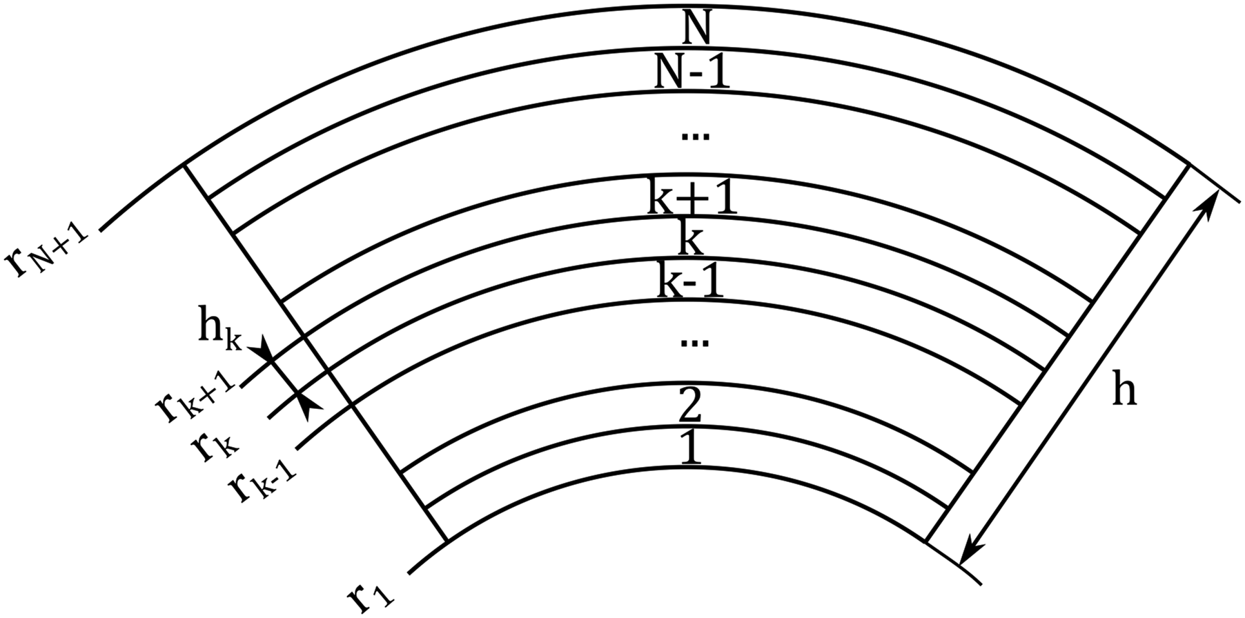
For a tube with a multi-layer structure the constants C₁, C₂ and A from the single-layer according to Lekhnitskii ² must be determined for each layer from k = 1 to k = N. The radial positions of the layer boundaries can be described by the respective inner radius r _k , outer radius r_k+1 and layer thickness h _k , see Figure 2. It should be noted that the indexing of the individual layers can be done in different ways. Almeida et al. ⁴ numbers the individual layers from the inside of the tube starting from one. The reference plane for the layer distances is the mid-plane of the tube segment section, based on which the distances t _i are given vectorially as a function of the z-axis, which is orthogonal to the laminate and oriented upwards. This definition can be used directly, for example, to determine the laminate properties using the Classical Laminate Theory (CLT). Often the z-axis in the CLT is defined for plates downwards in the laminate from the reference plane, cf. Gibson, ⁴² Ehrlich ⁴³ and Romano. ⁴⁴

Figure 2.

Indication of the layering with reference plane on the inner radius. ⁴⁵

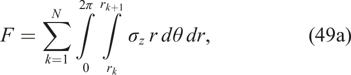
This results in a system of equations with 3N unknowns, which must be satisfied by 3(N − 1) boundary conditions at the interphases and 3 boundary conditions at the outer surfaces. The 3(N − 1) conditions on the interphases are denoted by

$\begin{array}{l}{\sigma }_r^k\left(r_{k+1}\right)={\sigma }_r^{k+1}\left(r_{k+1}\right),\\ {\tau }_{r\theta }^k\left(r_{k+1}\right)={\tau }_{r\theta }^{k+1}\left(r_{k+1}\right),\\ u_r^k\hspace{0.17em}\left(r_{k+1}\right)=u_r^{k+1}\left(r_{k+1}\right),\\ u_{\theta }^k\left(r_{k+1}\right)=u_{\theta }^{k+1}\left(r_{k+1}\right).\end{array}$

(33)

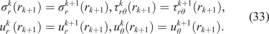
The stresses σ _r and τ _rθ yield an identical boundary condition, since their course is identical except for the sign and a phase shift. In addition, both stresses must become zero on the internal and external surface of the cylindrical tube and the bending moment corresponds to the summed surface integrals of the axial stress σ _z of all tube layers N. The three obtained boundary conditions are

$\begin{array}{l}{\sigma }_r^1\left(r_1\right)={\tau }_{r\theta }^1\left(r_1\right)=0,\\ {\sigma }_r^N\left(r_{N+1}\right)={\tau }_{r\theta }^N\left(r_{N+1}\right)=0,\\ M=2{\displaystyle \sum }_{k=1}^N\underset{0}{\overset{\pi }{{\displaystyle \int }}}\underset{r_k}{\overset{r_{k+1}}{{\displaystyle \int }}}{\sigma }_z^k\left(r,\theta \right)\hspace{0.17em}{r}^2\hspace{0.17em}\sin \hspace{0.17em}\theta \hspace{0.17em}dr\hspace{0.17em}d\theta .\end{array}$

(34)

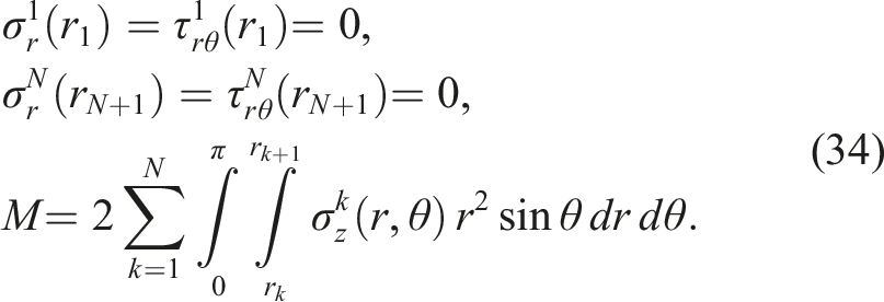
The equation for the bending moment can also be expressed by abbreviations of the coefficients of the unknowns according to the procedure for the displacements and stresses. This allows a conversion of the coefficents and boundary conditions into matrix notation and thus a linear system of equations for the three unknowns can be set up. ⁴⁰ Therefore, a simple calculation of the solution vector, containing all unknowns, is possible. Stresses, strains and displacements can be computed with known constants.

Multi-Layered tube according to Jolicoeur and Cardou

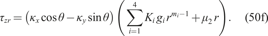
Unlike Xia et al., ³⁹ who are considering pure bending, Jolicoeur and Cardou ⁴⁶ use a more general formulation of the multi-layer tube based on the Lekhnitskii ² model. Axisymmetric tensile and torsional loads are taken into account, even though there is no coupling with bending.

Reformulation of the governing equations

The global constitutive law is used in monoclinic form, according to equation (3), with 13 independent elastic constants. The local constitutive law is not specified, but a permutation and transformation from a transversely isotropic fomulation is given by Siegl and Ehrlich. ³ The procedure of Jolicoeur and Cardou ⁴⁶ follows the approach of Lekhnitskii, except for a reformulation of the initial function for the axial strain ɛ _z as a function of the constant curvatures κ _x and κ _y as well as the nominal axial strain ɛ due to axial loads. Equation (9) then follows to

${\epsilon }_z={\kappa }_x\hspace{0.17em}r\hspace{0.17em}\sin \hspace{0.17em}\theta -{\kappa }_y\hspace{0.17em}r\hspace{0.17em}\cos \hspace{0.17em}\theta +\epsilon .$

(35)

A comparison of equations (9) and (35) provides the relations κ _x = A/S₃₃, κ _y = − B/S₃₃ and ɛ = C/S₃₃. Using this reformulated approach and the global monoclinic constitutive law, the governing system of equations (15a) and (15b) is simplified to

$\begin{array}{l}{L}_4^I\hspace{0.17em}F+L_3^I\hspace{0.17em}\mathrm{\Psi }=\frac{2}{r}\hspace{0.17em}\frac{S_{13}-S_{23}}{S_{33}}\hspace{0.17em}\left({\kappa }_x\hspace{0.17em}\sin \hspace{0.17em}\theta -{\kappa }_y\hspace{0.17em}\cos \hspace{0.17em}\theta \right),\\ L_3^{II}\hspace{0.17em}F+L_2^I\hspace{0.17em}\mathrm{\Psi }=\frac{S_{34}}{S_{33}}\hspace{0.17em}\left(2\hspace{0.17em}{\kappa }_x\hspace{0.17em}\sin \hspace{0.17em}\theta -2\hspace{0.17em}{\kappa }_y\hspace{0.17em}\cos \hspace{0.17em}\theta +\frac{\epsilon }{r}\right)-2\hspace{0.17em}\vartheta ,\end{array}$

(36)

using differential operators

$L_2^I=-{\beta }_{44}\hspace{0.17em}\frac{{\partial }^2}{\partial r^2}-{\beta }_{55}\hspace{0.17em}\frac{1}{r^2}\hspace{0.17em}\frac{{\partial }^2}{\partial {\theta }^2}-{\beta }_{44}\hspace{0.17em}\frac{1}{r}\hspace{0.17em}\frac{\partial }{\partial r},$

(37a)

$\begin{array}{l}{L}_3^I={\beta }_{24}\hspace{0.17em}\frac{{\partial }^3}{\partial r^3}+\left({\beta }_{14}+{\beta }_{56}\right)\hspace{0.17em}\frac{1}{r^2}\hspace{0.17em}\frac{{\partial }^3}{\partial r\partial {\theta }^2}\\ +\left({\beta }_{14}-2\hspace{0.17em}{\beta }_{24}\right)\hspace{0.17em}\frac{1}{r}\hspace{0.17em}\frac{{\partial }^2}{\partial r^2},\end{array}$

(37b)

$\begin{array}{l}{L}_3^{II}={\beta }_{24}\hspace{0.17em}\frac{{\partial }^3}{\partial r^3}+\left({\beta }_{14}+{\beta }_{56}\right)\hspace{0.17em}\frac{1}{r^2}\hspace{0.17em}\frac{{\partial }^3}{\partial r\partial {\theta }^2}\\ +\left({\beta }_{14}+{\beta }_{24}\right)\hspace{0.17em}\frac{1}{r}\hspace{0.17em}\frac{{\partial }^2}{\partial r^2}-\left({\beta }_{14}+{\beta }_{56}\right)\hspace{0.17em}\frac{1}{r^3}\hspace{0.17em}\frac{{\partial }^2}{\partial {\theta }^2},\end{array}$

(37c)

$\begin{array}{l}{L}_4^I=-{\beta }_{22}\hspace{0.17em}\frac{{\partial }^4}{\partial r^4}-\left(2\hspace{0.17em}{\beta }_{12}+{\beta }_{66}\right)\hspace{0.17em}\frac{1}{r^2}\hspace{0.17em}\frac{{\partial }^4}{\partial r^2\partial {\theta }^2}\\ -{\beta }_{11}\hspace{0.17em}\frac{1}{r^4}\hspace{0.17em}\frac{{\partial }^4}{\partial {\theta }^4}-2\hspace{0.17em}{\beta }_{22}\hspace{0.17em}\frac{1}{r}\hspace{0.17em}\frac{{\partial }^3}{\partial r^3}\\ +\left(2\hspace{0.17em}{\beta }_{12}+{\beta }_{66}\right)\hspace{0.17em}\frac{1}{r^3}\hspace{0.17em}\frac{{\partial }^3}{\partial r\partial {\theta }^2}+{\beta }_{11}\hspace{0.17em}\frac{1}{r^2}\hspace{0.17em}\frac{{\partial }^2}{\partial r^2}\\ -\left(2\hspace{0.17em}{\beta }_{11}+2\hspace{0.17em}{\beta }_{12}+{\beta }_{66}\right)\hspace{0.17em}\frac{1}{r^4}\hspace{0.17em}\frac{{\partial }^2}{\partial {\theta }^2}-{\beta }_{11}\hspace{0.17em}\frac{1}{r^3}\hspace{0.17em}\frac{\partial }{\partial r}.\end{array}$

(37d)

Here, the additional term ϑ is introduced, which symbolizes the relative twisting angle due to a torsional load. The superscripts () ^I and () ^II are used for numbering, whereas the subscripts represent the order.

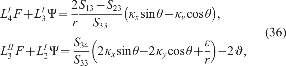
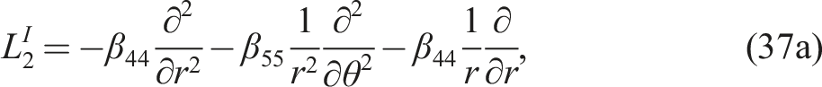
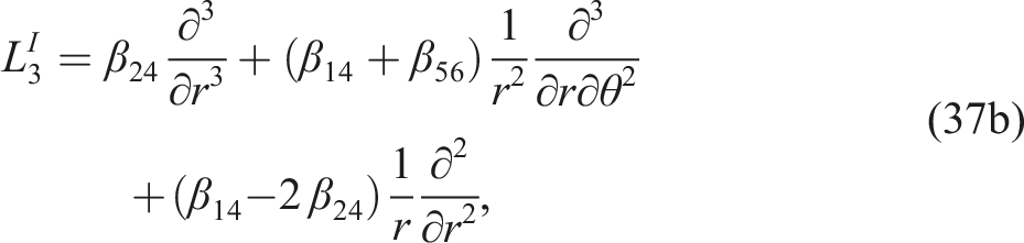
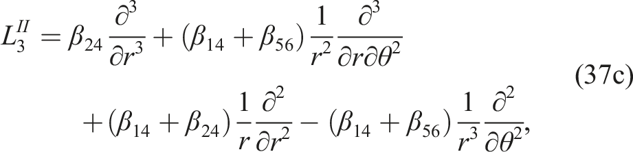
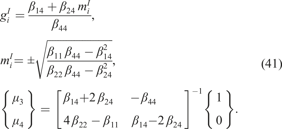
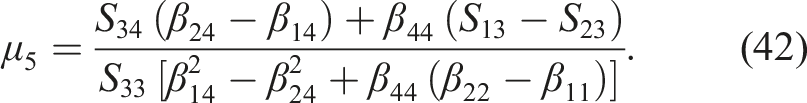
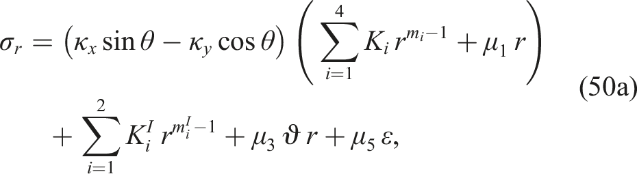
General solution of governing equations

A trigonometric solution f₁(r) and ϕ₁(r) for bending loads in dependence of the curvatures and a constant solution f₂(r) and ϕ₂(r) for axisymmetric loads are sought separately and then added up in the form

$\begin{array}{l}F=f_1\left(r\right)\hspace{0.17em}\left({\kappa }_x\hspace{0.17em}\sin \hspace{0.17em}\theta -{\kappa }_y\hspace{0.17em}\cos \hspace{0.17em}\theta \right)+f_2\left(r\right),\\ \mathrm{\Psi }={\varphi }_1\left(r\right)\hspace{0.17em}\left({\kappa }_x\hspace{0.17em}\sin \hspace{0.17em}\theta -{\kappa }_y\hspace{0.17em}\cos \hspace{0.17em}\theta \right)+{\varphi }_2\left(r\right).\end{array}$

(38)

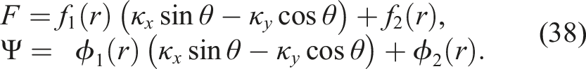
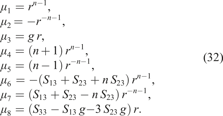
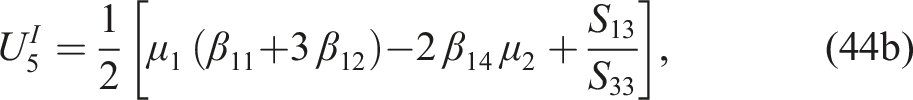
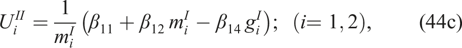
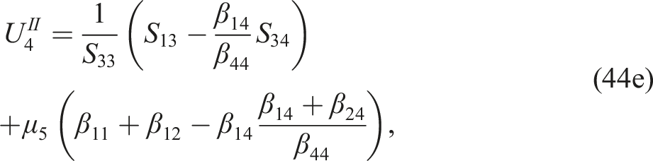
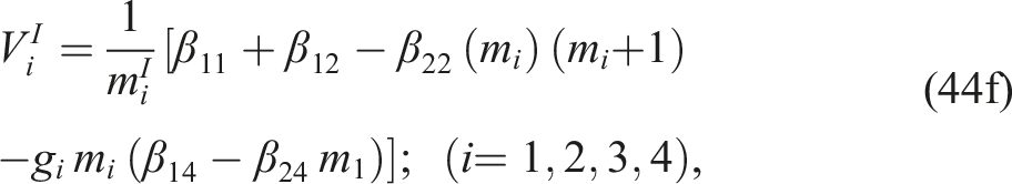
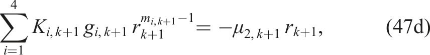
For each load case, homogeneous and particulate solutions are searched for the two functions and subsequently superposed. The general solution for the stress functions results after inserting equations (37) and (38) into equation (36) according to Jolicoeur and Cardou ⁴⁶ in

$\begin{array}{l}F=\left(\sum _{i=1}^4\frac{K_i}{m_i}\hspace{0.17em}{r}^{m_i+1}+K_5\hspace{0.17em}r+K_6\hspace{0.17em}r\hspace{0.17em}\ln \hspace{0.17em}r+\frac{{\mu }_1}{2}\hspace{0.17em}{r}^3\right)\\ \cdot \left({\kappa }_x\hspace{0.17em}\sin \hspace{0.17em}\theta -{\kappa }_y\hspace{0.17em}\cos \hspace{0.17em}\theta \right)+\sum _{i=1}^2\frac{K_i^I}{m_i^I+1}\hspace{0.17em}{r}^{m_i^I+1}\\ +K_3^I+K_4^I\hspace{0.17em}r+\frac{K_5^I}{2}\hspace{0.17em}{r}^2+\frac{{\mu }_3}{3}\hspace{0.17em}\vartheta \hspace{0.17em}{r}^3,\\ \mathrm{\Psi }=\left(\sum _{i=1}^4{K}_i\hspace{0.17em}{g}_i\hspace{0.17em}{r}^{m_i}+K_6\hspace{0.17em}\frac{{\beta }_{56}}{{\beta }_{66}}+{\mu }_2\hspace{0.17em}{r}^2\right)\hspace{0.17em}\left({\kappa }_x\hspace{0.17em}\sin \hspace{0.17em}\theta -{\kappa }_y\hspace{0.17em}\cos \hspace{0.17em}\theta \right)\\ +\sum _{i=1}^2\frac{K_i^I\hspace{0.17em}{g}_i^I}{m_i^I}\hspace{0.17em}{r}^{m_i^I}+K_4^I\hspace{0.17em}\frac{{\beta }_{11}}{{\beta }_{14}}\hspace{0.17em}\ln \hspace{0.17em}r+K_5^I\hspace{0.17em}\frac{{\beta }_{14}+{\beta }_{24}}{{\beta }_{44}}\hspace{0.17em}r\\ +K_6^I+\frac{S_{34}}{S_{33}{\beta }_{44}}\epsilon r+\frac{{\mu }_4}{2}\vartheta r^2.\end{array}$

(39)

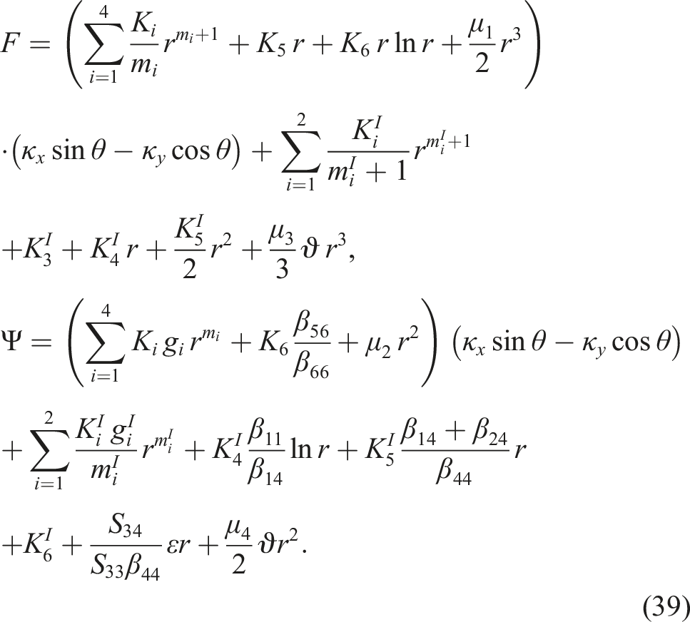
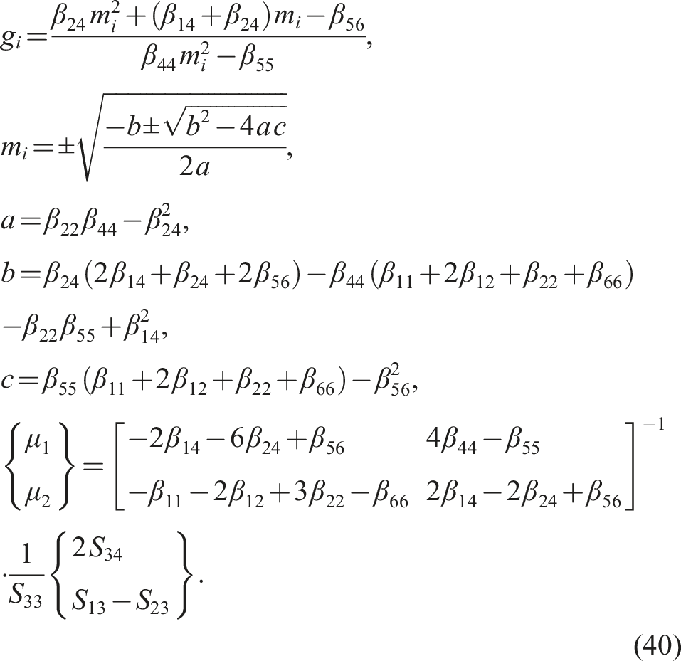
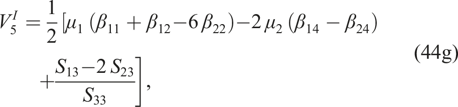
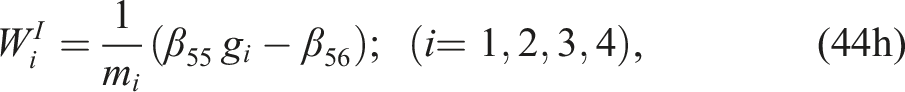
K _i for i = 1-6 represents the integration constants. The abbreviations g _i and m _i for i = 1-4 from the homogeneous solution as well as μ₁ and μ₂ from the particulate solution under pure bending are

$\begin{array}{l}{g}_i=\frac{{\beta }_{24}\hspace{0.17em}{m}_i^2+\left({\beta }_{14}+{\beta }_{24}\right)\hspace{0.17em}{m}_i-{\beta }_{56}}{{\beta }_{44}\hspace{0.17em}{m}_i^2-{\beta }_{55}},\\ m_i=\pm \sqrt{\frac{-b\pm \sqrt{b^2-4\hspace{0.17em}a\hspace{0.17em}c}}{2\hspace{0.17em}a}},\\ a={\beta }_{22}\hspace{0.17em}{\beta }_{44}-{\beta }_{24}^2,\\ b={\beta }_{24}\hspace{0.17em}\left(2\hspace{0.17em}{\beta }_{14}+{\beta }_{24}+2\hspace{0.17em}{\beta }_{56}\right)-{\beta }_{44}\hspace{0.17em}\left({\beta }_{11}+2\hspace{0.17em}{\beta }_{12}+{\beta }_{22}+{\beta }_{66}\right)\\ -{\beta }_{22}\hspace{0.17em}{\beta }_{55}+{\beta }_{14}^2,\\ c={\beta }_{55}\hspace{0.17em}\left({\beta }_{11}+2\hspace{0.17em}{\beta }_{12}+{\beta }_{22}+{\beta }_{66}\right)-{\beta }_{56}^2,\\ \left\{\begin{array}{l}{\mu }_1\\ {\mu }_2\end{array}\right\}={\left[\begin{array}{ll}-2\hspace{0.17em}{\beta }_{14}-6\hspace{0.17em}{\beta }_{24}+{\beta }_{56}& 4\hspace{0.17em}{\beta }_{44}-{\beta }_{55}\\ -{\beta }_{11}-2\hspace{0.17em}{\beta }_{12}+3\hspace{0.17em}{\beta }_{22}-{\beta }_{66}& 2\hspace{0.17em}{\beta }_{14}-2\hspace{0.17em}{\beta }_{24}+{\beta }_{56}\end{array}\right]}^{-1}\\ \cdot \frac{1}{S_{33}}\hspace{0.17em}\left\{\begin{array}{l}2\hspace{0.17em}{S}_{34}\\ S_{13}-S_{23}\end{array}\right\}.\end{array}$

(40)

The abbreviations $g_i^I$ and $m_i^I$ for i = 1-2 from the homogenous solution as well as μ₃ and μ₄ from the particulate solution under axisymmetric loads are

$\begin{array}{l}{g}_i^I=\frac{{\beta }_{14}+{\beta }_{24}\hspace{0.17em}{m}_i^I}{{\beta }_{44}},\\ m_i^I=\pm \sqrt{\frac{{\beta }_{11}\hspace{0.17em}{\beta }_{44}-{\beta }_{14}^2}{{\beta }_{22}\hspace{0.17em}{\beta }_{44}-{\beta }_{24}^2}},\\ \left\{\begin{array}{l}{\mu }_3\\ {\mu }_4\end{array}\right\}={\left[\begin{array}{ll}{\beta }_{14}+2\hspace{0.17em}{\beta }_{24}& -{\beta }_{44}\\ 4\hspace{0.17em}{\beta }_{22}-{\beta }_{11}& {\beta }_{14}-2\hspace{0.17em}{\beta }_{24}\end{array}\right]}^{-1}\left\{\begin{array}{l}1\\ 0\end{array}\right\}.\end{array}$

(41)

The unknowns K₅, $K_3^I$ and $K_6^I$ are set to zero because their associated stresses disappear when they are derived. ⁴⁶ Compliance of the fourth equation of the reduced constitutive law (10) leads to K₆ = 0 and the condition that the displacements are single-valued functions to $K_4^I=0$ and $K_5^I=\epsilon \hspace{0.17em}{\mu }_5$ with

${\mu }_5=\frac{S_{34}\hspace{0.17em}\left({\beta }_{24}-{\beta }_{14}\right)+{\beta }_{44}\hspace{0.17em}\left(S_{13}-S_{23}\right)}{S_{33}\hspace{0.17em}\left[{\beta }_{14}^2-{\beta }_{24}^2+{\beta }_{44}\hspace{0.17em}\left({\beta }_{22}-{\beta }_{11}\right)\right]}.$

(42)

Stresses are obtained by substituting equation (39) into (12). Strains and displacements can be expressed using the fundamental equations. The previously unknown terms U _r , U _θ and U _z from (14) follow to

$\begin{array}{l}{U}_r=\left({\kappa }_x\hspace{0.17em}\sin \hspace{0.17em}\theta -{\kappa }_y\hspace{0.17em}\cos \hspace{0.17em}\theta \right)\hspace{0.17em}\left({\displaystyle \sum }_{i=1}^4{K}_i\hspace{0.17em}{U}_i^I\hspace{0.17em}{r}^{m_i}+U_5^I\hspace{0.17em}{r}^2\right)\\ +{\displaystyle \sum }_{i=1}^2{K}_i^I\hspace{0.17em}{U}_i^{II}\hspace{0.17em}{r}^{m_i}+U_3^{II}\hspace{0.17em}\vartheta \hspace{0.17em}{r}^2+U_4^{II}\hspace{0.17em}\epsilon \hspace{0.17em}r,\\ U_{\theta }=\left({\kappa }_x\hspace{0.17em}\cos \hspace{0.17em}\theta +{\kappa }_y\hspace{0.17em}\sin \hspace{0.17em}\theta \right)\hspace{0.17em}\left({\displaystyle \sum }_{i=1}^4{K}_i\hspace{0.17em}{V}_i^I\hspace{0.17em}{r}^{m_i}+V_5^I\hspace{0.17em}{r}^2\right),\\ U_z=\left({\kappa }_x\hspace{0.17em}\cos \hspace{0.17em}\theta +{\kappa }_y\hspace{0.17em}\sin \hspace{0.17em}\theta \right)\hspace{0.17em}\left({\displaystyle \sum }_{i=1}^4{K}_i\hspace{0.17em}{W}_i^I\hspace{0.17em}{r}^{m_i}+W_5^I\hspace{0.17em}{r}^2\right),\end{array}$

(43)

with the subexpressions

$U_i^I=\frac{1}{m_i}\hspace{0.17em}\left[{\beta }_{11}+{\beta }_{12}\hspace{0.17em}\left(m_i+1\right)-{\beta }_{14}\hspace{0.17em}{g}_i\hspace{0.17em}{m}_i\right];\left(i=\mathrm{1,2,3,4}\right),$

(44a)

$U_5^I=\frac{1}{2}\hspace{0.17em}\left[{\mu }_1\hspace{0.17em}\left({\beta }_{11}+3\hspace{0.17em}{\beta }_{12}\right)-2\hspace{0.17em}{\beta }_{14}\hspace{0.17em}{\mu }_2+\frac{S_{13}}{S_{33}}\right],$

(44b)

$U_i^{II}=\frac{1}{m_i^I}\hspace{0.17em}\left({\beta }_{11}+{\beta }_{12}\hspace{0.17em}{m}_i^I-{\beta }_{14}\hspace{0.17em}{g}_i^I\right);\left(i=\mathrm{1,2}\right),$

(44c)

$U_3^{II}=\frac{1}{2}\hspace{0.17em}\left[{\mu }_3\hspace{0.17em}\left({\beta }_{11}+2\hspace{0.17em}{\beta }_{12}\right)-{\mu }_4\hspace{0.17em}{\beta }_{14}\right],$

(44d)

$\begin{array}{l}{U}_4^{II}=\frac{1}{S_{33}}\hspace{0.17em}\left(S_{13}-\frac{{\beta }_{14}}{{\beta }_{44}}\hspace{0.17em}{S}_{34}\right)\\ +{\mu }_5\hspace{0.17em}\left({\beta }_{11}+{\beta }_{12}-{\beta }_{14}\hspace{0.17em}\frac{{\beta }_{14}+{\beta }_{24}}{{\beta }_{44}}\right),\end{array}$

(44e)

$\begin{array}{l}{V}_i^I=\frac{1}{m_i^I}\hspace{0.17em}[{\beta }_{11}+{\beta }_{12}-{\beta }_{22}\hspace{0.17em}\left(m_i\right)\hspace{0.17em}\left(m_i+1\right)\\ -g_i\hspace{0.17em}{m}_i\hspace{0.17em}\left({\beta }_{14}-{\beta }_{24}\hspace{0.17em}{m}_1\right)];\left(i=\mathrm{1,2,3,4}\right),\end{array}$

(44f)

$\begin{array}{l}{V}_5^I=\frac{1}{2}\hspace{0.17em}[{\mu }_1\hspace{0.17em}\left({\beta }_{11}+{\beta }_{12}-6\hspace{0.17em}{\beta }_{22}\right)-2\hspace{0.17em}{\mu }_2\hspace{0.17em}\left({\beta }_{14}-{\beta }_{24}\right)\\ +\frac{S_{13}-2\hspace{0.17em}{S}_{23}}{S_{33}}],\end{array}$

(44g)

$W_i^I=\frac{1}{m_i}\hspace{0.17em}\left({\beta }_{55}\hspace{0.17em}{g}_i-{\beta }_{56}\right);\left(i=\mathrm{1,2,3,4}\right),$

(44h)

$W_5^I=\frac{1}{2}\hspace{0.17em}\left({\beta }_{55}\hspace{0.17em}{\mu }_2-{\beta }_{56}\hspace{0.17em}{\mu }_1\right).$

(44i)

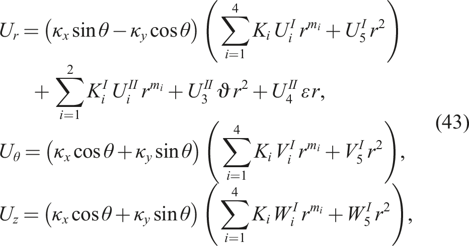
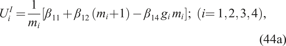
These are explicitly mentioned at this point because they are necessary for establishing the continuity conditions and the determination of the remaining unknown constants K₁-K₄ as well as $K_1^I$ - $K_2^I$ . The function U _z represents warping and rotation of the cross section, wherefore the Euler-Bernoulli hypothesis is not applicable. ⁴⁷

Enhancements to the multi-layer composite

Rigid body motions, see equation (14), are usually set equal to zero for this kind of problem, but here the two translational components u₀ and v₀ are required to take the effect of Poisson ratios into account. ⁴⁶ They can be expressed by an unknown constant ν and the curvatures as

$u_0=-\nu \hspace{0.17em}{\kappa }_y;v_0=\nu \hspace{0.17em}{\kappa }_x$

(45)

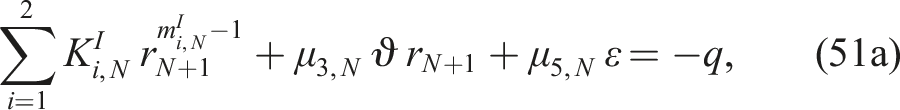
To determine the unknown constants, Jolicoeur and Cardou ⁴⁶ distinguish two cases of boundary conditions between the individual layers: ’No Slip’, or rather ’Perfect Bonding’, and ’No Friction’. In the first case all displacements u _r , u _θ and u _z as well as the radial stress components σ _r , τ _rθ and τ _rz are considered to be continous and all single layers are in contact, which implies sufficient prestress. Therefore seven conditions, because continuity of u _r leads to two different equations, for the interphases can be established to

$\begin{array}{l}{\displaystyle \sum }_{i=1}^4{K}_{i,k}\hspace{0.17em}{r}_{k+1}^{m_{i,k}-1}-K_{i,k+1}\hspace{0.17em}{r}_{k+1}^{m_{i,k+1}-1}\\ =\left({\mu }_{1,k+1}-{\mu }_{1,k}\right)\hspace{0.17em}{r}_{k+1},\end{array}$

(46a)

$\begin{array}{l}{\displaystyle \sum }_{i=1}^2{K}_{i,k}^I\hspace{0.17em}{r}_{k+1}^{m_{i,k}^I-1}-K_{i,k+1}^I\hspace{0.17em}{r}_{k+1}^{m_{i,k+1}^I-1}\\ =\left({\mu }_{3,k+1}-{\mu }_{3,k}\right)\hspace{0.17em}\vartheta \hspace{0.17em}{r}_{k+1}+\left({\mu }_{5,k+1}-{\mu }_{5,k}\right)\hspace{0.17em}\epsilon ,\end{array}$

(46b)

$\begin{array}{l}{\displaystyle \sum }_{i=1}^4{K}_{i,k}\hspace{0.17em}{g}_{i,k}\hspace{0.17em}{r}_{k+1}^{m_{i,k}-1}-K_{i,k+1}\hspace{0.17em}{g}_{i,k+1}\hspace{0.17em}{r}_{k+1}^{m_{i,k+1}-1}\\ =\left({\mu }_{2,k+1}-{\mu }_{2,k}\right)\hspace{0.17em}{r}_{k+1},\end{array}$

(46c)

$\begin{array}{l}{\nu }_k-{\nu }_{k+1}+{\displaystyle \sum }_{i=1}^4{K}_{i,k}\hspace{0.17em}{U}_{i,k}^I\hspace{0.17em}{r}_{k+1}^{m_{i,k}}-K_{i,k+1}\hspace{0.17em}{U}_{i,k+1}^I\hspace{0.17em}{r}_{k+1}^{m_{i,k+1}}\\ =\left(U_{5,k+1}^I-U_{5,k}^I\right)\hspace{0.17em}{r}_{k+1}^2,\end{array}$

(46d)

$\begin{array}{l}{\displaystyle \sum }_{i=1}^2{K}_{i,k}^I\hspace{0.17em}{U}_{i,k}^{II}\hspace{0.17em}{r}_{k+1}^{m_{i,k}^I}-K_{i,k+1}^I\hspace{0.17em}{U}_{i,k+1}^{II}\hspace{0.17em}{r}_{k+1}^{m_{i,k+1}^I}\\ =\left(U_{3,k+1}^{II}-U_{3,k}^{II}\right)\hspace{0.17em}\vartheta \hspace{0.17em}{r}_{k+1}^2+\left(U_{4,k+1}^{II}-U_{4,k}^{II}\right)\hspace{0.17em}\epsilon \hspace{0.17em}{r}_{k+1},\end{array}$

(46e)

$\begin{array}{l}{\nu }_k-{\nu }_{k+1}+{\displaystyle \sum }_{i=1}^4{K}_{i,k}\hspace{0.17em}{V}_{i,k}^I{r}_{k+1}^{m_{i,k}}-K_{i,k+1}\hspace{0.17em}{V}_{i,k+1}^I\hspace{0.17em}{r}_{k+1}^{m_{i,k+1}}\\ =\left(V_{5,k+1}^I-V_{5,k}^I\right)\hspace{0.17em}{r}_{k+1}^2,\end{array}$

(46f)

$\begin{array}{l}{\displaystyle \sum }_{i=1}^4{K}_{i,k}\hspace{0.17em}{W}_{i,k}^I{r}_{k+1}^{m_{i,k}}-K_{i,k+1}\hspace{0.17em}{W}_{i,k+1}^I\hspace{0.17em}{r}_{k+1}^{m_{i,k+1}}\\ =\left(W_{5,k+1}^I-W_{5,k}^I\right)\hspace{0.17em}{r}_{k+1}^2\end{array}$

(46g)

In the second case of ’No Friction’, a sliding of the single layers along θ and z on the interphases is allowed. Hence, the displacements u _θ and u _z can be discontinous and the stresses τ _rθ and τ _rz become zero on the layer boundaries. This leads to the following four conditions

${\displaystyle \sum }_{i=1}^4{K}_{i,k}\hspace{0.17em}{r}_{k+1}^{m_{i,k}-1}=-{\mu }_{1,k}\hspace{0.17em}{r}_{k+1},$

(47a)

${\displaystyle \sum }_{i=1}^4{K}_{i,k+1}\hspace{0.17em}{r}_{k+1}^{m_{i,k+1}-1}=-{\mu }_{1,k+1}\hspace{0.17em}{r}_{k+1},$

(47b)

${\displaystyle \sum }_{i=1}^4{K}_{i,k}\hspace{0.17em}{g}_{i,k}\hspace{0.17em}{r}_{k+1}^{m_{i,k}-1}=-{\mu }_{2,k}\hspace{0.17em}{r}_{k+1},$

(47c)

${\displaystyle \sum }_{i=1}^4{K}_{i,k+1}\hspace{0.17em}{g}_{i,k+1}\hspace{0.17em}{r}_{k+1}^{m_{i,k+1}-1}=-{\mu }_{2,k+1}\hspace{0.17em}{r}_{k+1},$

(47d)

which are used in addition to the already established equations (46b), (46d) and (46e). Thus, 7(N − 1) conditions exist regardless of the contact type for 7N unknowns K_1,k-K_4,k, $K_{1,k}^I$ - $K_{2,k}^I$ and ν _k . The remaining boundary conditions of σ _r = τ _rθ = τ _rz = 0 on the outer and inner surface of the tube are providing the remaining seven equations with (47a) and (47c) for r₁ and r_N+1 as well as

${\displaystyle \sum }_{i=1}^2{K}_{i,N}^I\hspace{0.17em}{r}_{N+1}^{m_{i,N}^I-1}=-{\mu }_{3,N}\hspace{0.17em}\vartheta \hspace{0.17em}{r}_{N+1}-{\mu }_{5,N}\hspace{0.17em}\epsilon ,$

(48a)

${\displaystyle \sum }_{i=1}^2{K}_{i,1}^I\hspace{0.17em}{r}_1^{m_{i,1}^I-1}=-{\mu }_{\mathrm{3,1}}\hspace{0.17em}\vartheta \hspace{0.17em}{r}_1-{\mu }_{\mathrm{5,1}}\hspace{0.17em}\epsilon .$

(48b)

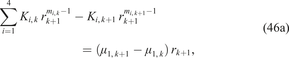
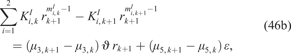
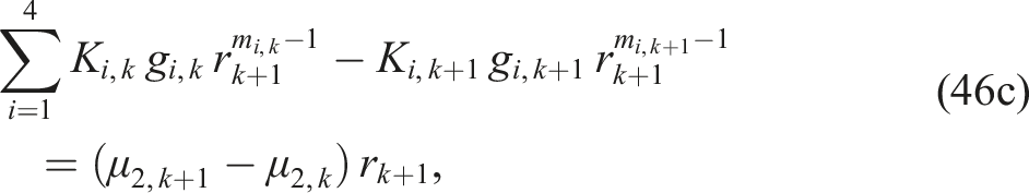
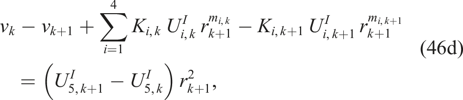
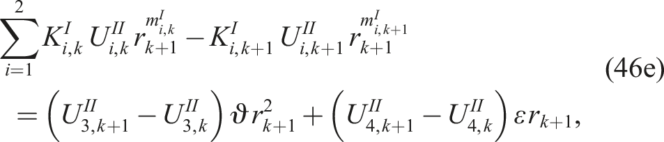
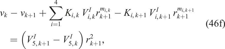
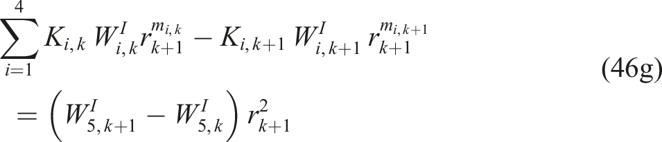
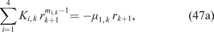
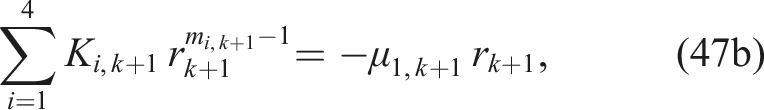
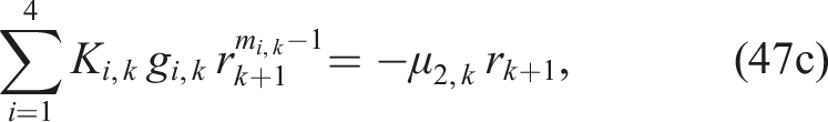
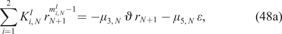
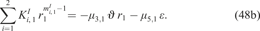
The constant ν₁ is set equal to zero for the first layer to gain the seventh equation. The obtained system of linear equations is divided into two subsystems. Firstly, the subsystem for bending loads is build using either interphase conditions (46a), (46c), (46d), (46f) and (46g) for ’No Slip’ or (46d) and (47a-47d) for ’No Friction’ to obtain K_1,k-K_4,k and ν _k . Equations (47a) and (47c) are used on the external surfaces independent of the interphase boundary conditions. Secondly, the subsystem for axisymmetric loads and the determination of $K_1^I$ - $K_2^I$ can regardless of the contact type be solved for known ɛ and ϑ using equations (46b), (46e) on the interphases and (48a), (48b) on the external surfaces. The external force F and moments T, M _x , M _y are expressed by the summation of surface integrals of the cross sections of each individual layer by

$F={\displaystyle \sum }_{k=1}^N\underset{0}{\overset{2\pi }{{\displaystyle \int }}}\underset{r_k}{\overset{r_{k+1}}{{\displaystyle \int }}}{\sigma }_z\hspace{0.17em}r\hspace{0.17em}d\theta \hspace{0.17em}dr,$

(49a)

$T={\displaystyle \sum }_{k=1}^N\underset{0}{\overset{2\pi }{{\displaystyle \int }}}\underset{r_k}{\overset{r_{k+1}}{{\displaystyle \int }}}{\tau }_{\theta z}\hspace{0.17em}{r}^2\hspace{0.17em}d\theta \hspace{0.17em}dr,$

(49b)

$M_x={\displaystyle \sum }_{k=1}^N\underset{0}{\overset{2\pi }{{\displaystyle \int }}}\underset{r_k}{\overset{r_{k+1}}{{\displaystyle \int }}}{\sigma }_z\hspace{0.17em}{r}^2\hspace{0.17em}\sin \hspace{0.17em}\theta \hspace{0.17em}d\theta \hspace{0.17em}dr,$

(49c)

$M_y=-{\displaystyle \sum }_{k=1}^N\underset{0}{\overset{2\pi }{{\displaystyle \int }}}\underset{r_k}{\overset{r_{k+1}}{{\displaystyle \int }}}{\sigma }_z\hspace{0.17em}{r}^2\hspace{0.17em}\cos \hspace{0.17em}\theta \hspace{0.17em}d\theta \hspace{0.17em}dr.$

(49d)

The equations associated with the respective loads are integrated into the corresponding linear equation system. Both can be solved separately using matrix form. There is no coupling between axisymmetric loads and bending loads. This also applies to the bending moment M _x and the curvature κ _y and vice versa. ⁴⁶ In addition, both curvatures are constant along the z axis. The solution procedure ist similar to the previously described procedure according Xia et al. ³⁹ The final stresses according to Jolicoeur and Cardou ⁴⁶ result in

$\begin{array}{l}{\sigma }_r=\left({\kappa }_x\hspace{0.17em}\sin \hspace{0.17em}\theta -{\kappa }_y\hspace{0.17em}\cos \hspace{0.17em}\theta \right)\hspace{0.17em}\left({\displaystyle \sum }_{i=1}^4{K}_i\hspace{0.17em}{r}^{m_i-1}+{\mu }_1\hspace{0.17em}r\right)\\ +{\displaystyle \sum }_{i=1}^2{K}_i^I\hspace{0.17em}{r}^{m_i^I-1}+{\mu }_3\hspace{0.17em}\vartheta \hspace{0.17em}r+{\mu }_5\hspace{0.17em}\epsilon ,\end{array}$

(50a)

$\begin{array}{l}{\sigma }_{\theta }=\left({\kappa }_x\hspace{0.17em}\sin \hspace{0.17em}\theta -{\kappa }_y\hspace{0.17em}\cos \hspace{0.17em}\theta \right)\hspace{0.17em}\left({\displaystyle \sum }_{i=1}^4{K}_i\hspace{0.17em}\left(m_i+1\right)\hspace{0.17em}{r}^{m_i-1}+3\hspace{0.17em}{\mu }_1\hspace{0.17em}r\right)\\ +{\displaystyle \sum }_{i=1}^2{K}_i^I\hspace{0.17em}{m}_i^I\hspace{0.17em}{r}^{m_i^I-1}+2\hspace{0.17em}{\mu }_3\hspace{0.17em}\vartheta \hspace{0.17em}r+{\mu }_5\hspace{0.17em}\epsilon ,\end{array}$

(50b)

${\sigma }_z=\frac{1}{S_{33}}\hspace{0.17em}\left[{\kappa }_x\hspace{0.17em}r\hspace{0.17em}\sin \hspace{0.17em}\theta -{\kappa }_y\hspace{0.17em}r\hspace{0.17em}\cos \hspace{0.17em}\theta +\epsilon -S_{13}\hspace{0.17em}{\sigma }_r-S_{23}\hspace{0.17em}{\sigma }_{\theta }-S_{34}\hspace{0.17em}{\tau }_{\theta z}\right],$

(50c)

${\tau }_{r\theta }=\left({\kappa }_x\hspace{0.17em}\cos \hspace{0.17em}\theta -{\kappa }_y\hspace{0.17em}\sin \hspace{0.17em}\theta \right)\hspace{0.17em}\left(-{\displaystyle \sum }_{i=1}^4{K}_i\hspace{0.17em}{r}^{m_i-1}-{\mu }_1\hspace{0.17em}r\right),$

(50d)

$\begin{array}{l}{\tau }_{\theta z}=\left({\kappa }_x\hspace{0.17em}\sin \hspace{0.17em}\theta -{\kappa }_y\hspace{0.17em}\cos \hspace{0.17em}\theta \right)\hspace{0.17em}\left(-{\displaystyle \sum }_{i=1}^4{K}_i\hspace{0.17em}{g}_i\hspace{0.17em}{m}_i\hspace{0.17em}{r}^{m_i-1}-2\hspace{0.17em}{\mu }_2\hspace{0.17em}r\right)\\ -{\displaystyle \sum }_{i=1}^2{K}_i^I\hspace{0.17em}{g}_i^I\hspace{0.17em}{r}^{m_i^I-1}-{\mu }_4\hspace{0.17em}\vartheta \hspace{0.17em}r-\left({\mu }_5\hspace{0.17em}\frac{{\beta }_{14}+{\beta }_{24}}{{\beta }_{44}}+\frac{S_{34}}{S_{33}+{\beta }_{44}}\right)\hspace{0.17em}\epsilon ,\end{array}$

(50e)

${\tau }_{zr}=\left({\kappa }_x\hspace{0.17em}\cos \hspace{0.17em}\theta -{\kappa }_y\hspace{0.17em}\sin \hspace{0.17em}\theta \right)\hspace{0.17em}\left({\displaystyle \sum }_{i=1}^4{K}_i\hspace{0.17em}{g}_i\hspace{0.17em}{r}^{m_i-1}+{\mu }_2\hspace{0.17em}r\right).$

(50f)

Further enhancements regarding tubes under bending loads

According to Zhang and Hoa ⁴¹ all models based on Lekhnitskii formalism share the disadvantage that, for C₃ ≠ 0 and fiber angles of 0° or 90°, fewer unknowns than equations are present and therefore several solutions for the stress field exist. While the models according to Lekhnitskii ² and Xia et al. ³⁹ circumvent this problem by the neglection of C₃, the model of Jolicoeur and Cardou ⁴⁶ is fully exposed to it. For example, the continuity conditions of τ _rz , τ _θz and u _z are satisfied identically and simplify to identities for K₃ ≠ 0. This drawback is solved by Zhang and Hoa ⁴¹ using a limit-based approach with an approximation by Taylor series of expansion for identically solved continuity conditions. In a subsequent paper by Zhang et al. ⁴⁸ this approach is advanced to composites with arbitrary lay-ups and fiber angles using the introduced unified and unknown coefficients $K_3^{*}$ and $K_4^{*}$ , which become K₃ and K₄ for fiber angles of neither 0° nor 90°. In the other case, these coefficients turn into approximated constants which are derived using the Taylor series of expansion for compliances, reduced compliances as well as all terms depending on them (i. e. g _i and m _i for i = 1, 2, 3, 4 and μ _i i = 1, 2). This includes the coefficients themselves.

Using a reformulation of the model of Xia et al., ³⁹ Menshykova and Guz ⁴⁹ examined the difference between an innermost metallic and an axially oriented carbon composite layer. In the model description, two winding layers are combined to an orthotropic layer [±α], a formulation of an isotropic layer is established and new abbreviations of the compliances are used for a better representation. A comparative study of the lay-ups [steel/±α/0] and [0/±α/0] under varying fiber angles α and pure bending is carried out using the program Matlab. The focus of this investigation lies on the normal stress curves across the thickness at the point θ = π/2 of the highest positive axial stress. The tubes have an internal radius of 2.5 mm and an external radius of 7.5 mm, making them thick-walled. Menshykova and Guz ⁴⁹ showed that an increase in the layer thickness of the innermost layer, steel and carbon composite, or a decrease in the fiber angle ±α of the central layer results in higher stress jumps between the layers. In addition, the isotropic innermost layer displaced the highest jump in the axial and circumferrential normal stresses from the transition between the ±α- and the outer 0°-layer to the transition between the inner, isotropic layer and the ±α-layer.

Based on the tube model of Jolicoeur and Cardou, ⁴⁶ and thus Lekhnitskii, ² Chouchaoui and Ochoa ⁴⁷ use a new variant of the boundary condition ’No Slip’ between the layers. In addition to the conditions of the underlying model that the stresses σ _r , τ _rθ , τ _rz and displacements u _r , u _θ , u _z show a continuous course over the thickness of the laminate, the shear stresses τ _rθ , τ _rz become zero at the interphases. Jolicoeur and Cardou ⁴⁶ more reasonably employed this zeroing in combination with allowing a slip and therefore discontinous course of displacements u _r and u _θ calling it ’No Friction’. So for the subsystem of linear equations and bending loads the conditions (47a-47d) are used in combination with (46d), (46f) and (46g) instead of (46a) and (46c) in the ’No Slip’ case of Jolicoeur and Cardou. ⁴⁶ Furthermore, for the model of Chouchaoui and Ochoa ⁴⁷ the radial stress σ _r at the outer surfaces corresponds to the respective internal or external pressure p or -q and does not become zero. This is taken into account in the boundary conditions (48a) and (48b) in the following way

$\begin{array}{l}{\displaystyle \sum }_{i=1}^2{K}_{i,N}^I\hspace{0.17em}{r}_{N+1}^{m_{i,N}^I-1}+{\mu }_{3,N}\hspace{0.17em}\vartheta \hspace{0.17em}{r}_{N+1}+{\mu }_{5,N}\hspace{0.17em}\epsilon \hspace{0.17em}=-q,\end{array}$

(51a)

$\begin{array}{l}{\displaystyle \sum }_{i=1}^2{K}_{i,1}^I\hspace{0.17em}{r}_1^{m_{i,1}^I-1}+{\mu }_{\mathrm{3,1}}\hspace{0.17em}\vartheta \hspace{0.17em}{r}_1+{\mu }_{\mathrm{5,1}}\hspace{0.17em}\epsilon \hspace{0.17em}=p\end{array}.$

(51b)

Further enhancements regarding tubes under axisymmetric loads

There are significantly more models dealing with axisymmetric loads and in particular internal pressure, than those dealing with bending loads. This is due to the further simplification of the uniform load over the circumferential direction θ and the frequent use of composites in pipeline and tank applications. The basic formulation can also be traced back to general and axisymmetric formulations by Lekhnitskii, ² but there are also approaches from laminated plate theories. The extension to the multi-layer composite of Jolicoeur and Cardou ⁴⁶ applies, as already described in the section Multi-Layered tube according to Jolicoeur and Cardou, for both bending and axisymmetric loads. They gave a more general formulation than Lekhnitskii, who separated each specific load case.

Furthermore, Ting ⁵⁰ developed a variant of the Lekhnitskii formulation for a single-layered tube with cylindrical anisotropy where stresses, strains and displacements only depend on the radial coordinate r. The model applies for given uniform stresses σ _r , τ _rθ , τ _rz on the external surfaces as well as a uniform axial strain or torsion. In contrast to Lekhnitskii, ² the compliance terms and therefore the constitutive law also occurs in a double-reduced form, which allows a more compact and simple system description. The two reductions are possible due to the specification of known deformations ɛ _z and γ _θr . The publication is an extension of an earlier publication by Ting, ⁵¹ which solves the same problem by using the Stroh ²⁶ formulation. The description, however, is less complex and physically more tangible. ⁵⁰

For the same model boundaries and load conditions, Chen et al. ⁵² have adapted the model of Ting ⁵¹ almost simultaneously to Ting ⁵⁰ into a Lekhnitskii formulation. As a novelty towards Ting, the load case of a constant temperature change is added and the system is described without the necessity of a superposition of the basic equations. This gives a more direct applicability.

Displacement-Based approaches

Displacement-based tube models, found in the literature, do not provide exact solutions in all coordinate directions for the load case of pure bending. However, the models of the state-space approach, which are presented in section State-Space Approaches, usually use a displacement approach in combination with stresses. In addition to a few short descriptions of models with axisymmetric loads, this section presents the displacement-based approximity solutions according to Sarvestani et al.^45,53–57 for tubes under different bending loads. Displacement-based approaches provide a compatible displacement field for the continuum derived from the fundamental equations, which must be solved to obtain strains and stresses.

Axisymmetric loads

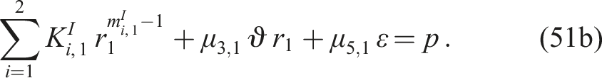
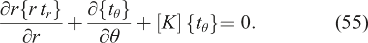
Ting ⁵¹ formulated a single-layered, orthotropic tube model based on the Stroh formulation for axisymmetric loads using a special matrix form for the equilibrium equations with the stress vectors

$\left\{t_r\right\}=\left\{\begin{array}{l}{\sigma }_r\\ {\tau }_{r\theta }\\ {\tau }_{rz}\end{array}\right\};\left\{t_{\theta }\right\}=\left\{\begin{array}{l}{\tau }_{\theta r}\\ {\sigma }_{\theta }\\ {\tau }_{\theta z}\end{array}\right\};\left\{t_z\right\}=\left\{\begin{array}{l}{\tau }_{zr}\\ {\tau }_{z\theta }\\ {\sigma }_z\end{array}\right\}$

(52)

and the coefficent matrix

$\left[K\right]=\left[\begin{array}{lll}0& -1& 0\\ 1& 0& 0\\ 0& 0& 0\end{array}\right]$

(53)

the equilibrium equation (5) can be represented by the matrix equation

$\frac{\partial r\left\{r\hspace{0.17em}{t}_r\right\}}{\partial r}+\frac{\partial \left\{t_{\theta }\right\}}{\partial \theta }+\left[K\right]\hspace{0.17em}\left\{t_{\theta }\right\}\hspace{0.17em}r\frac{\partial \left\{t_z\right\}}{\partial z}=0.$

(54)

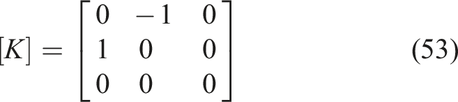
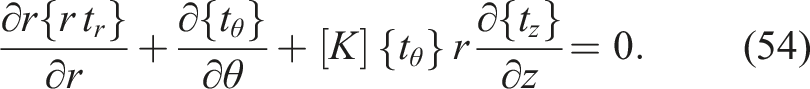
An independence of z simplifies this equation to

$\frac{\partial r\left\{r\hspace{0.17em}{t}_r\right\}}{\partial r}+\frac{\partial \left\{t_{\theta }\right\}}{\partial \theta }+\left[K\right]\hspace{0.17em}\left\{t_{\theta }\right\}=0.$

(55)

Using the strain-displacement relations (6), the three stress vectors can be related to the displacements via stiffness terms. If these relations are employed in equation (55) for cylindrical anisotropy, a single system of equations for the displacement vector {u} is obtained. In the used form, which is simplified to the sole dependence on coordinate r, this results in

$\begin{array}{l}r\hspace{0.17em}\left[Q\right]\hspace{0.17em}\frac{\partial r\hspace{0.17em}\frac{\partial \left\{u\right\}}{\partial r}}{\partial r}+r\hspace{0.17em}\left(\left[R\right]\hspace{0.17em}\left[K\right]+\left[K\right]\hspace{0.17em}{\left[R\right]}^T\right)\hspace{0.17em}\frac{\partial \left\{u\right\}}{\partial r}\\ +\left[K\right]\hspace{0.17em}\left[T\right]\hspace{0.17em}\left[K\right]\hspace{0.17em}\left\{u\right\}=0.\end{array}$

(56)

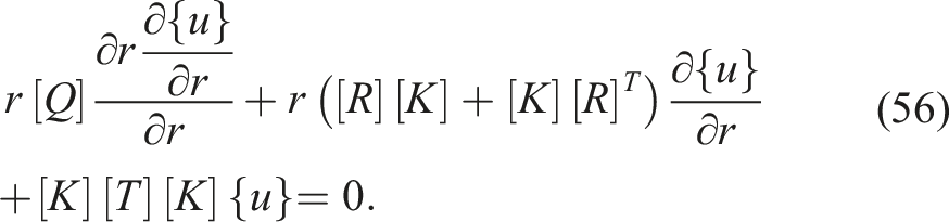
The matrices [Q] = [C_i1k1], [R] = [C_i1k2] and [T] = [C_i2k2] are submatrices of the stiffness matrix [C _ijkl ].

Substituting the equation (57) in equation (56) yields six eigenvalues and eigenvectors, which must be determined separately for each load case, taking into account the respective boundary conditions. A system of diffential equations depending on the displacement vector {u} is formed using these equilibrium equations, the kinematic relations and the full tensor notation of the material law. The solution is then searched in the form

$\left\{u\right\}=r^{{\lambda }_i}\left\{g_i\right\},$

(57)

where λ _i are eigenvalues and {g _i } eigenvectors of the system. For each load case these eigenvalues and -vectors are determined using boundary conditions. The load cases under consideration are internal and external pressure in radial direction, a predetermined shear load for τ _rθ and τ _rz on the inner and outer radius as well as torsional and axial extension, all distributed uniformly over the hoop direction θ. In the case of the latter two, a dependency on coordinate z is taken into account for the displacements but not for the stresses. For the respective load case, all six stress and three displacement curves can be calculated. A superposition of the results of the individual load cases is also possible.

A multi-layer tube model under internal pressure based on the classical laminated plate theory was developed by Xia et al. ⁵⁸ The fundamental equations are independent of z and θ, what simplifies them and the system of governing equations. This system of partial differential equations is described for the displacements u _r and u _θ using global stiffnesses [C _ij ] for (i, j = 1-6) in monotropic form. It is solved using continuity conditions for u _r , u _θ , σ _r , τ _rθ and τ _rz as well as boundary conditions σ _r (r₁) = − p and σ _r (r_N+1) = τ _rθ (r₁) = τ _rθ (r_N+1) = τ _rz (r₁) = τ _rz (r_N+1) = 0.

Zu et al. ⁵⁹ established a thick-walled, multi-layered tube model, defined by a ratio of radius to thickness of 10, under internal pressure and expanded it for an isotropic, metallic innermost layer. Compared to Xia et al., ⁵⁸ they simplified the model by neglecting the stresses τ _rθ , τ _rz and the related conditions. In analytical investigations the model was compared with the results of Xia et al. ⁵⁸ and the influence of the metallic inner layer was investigated. Adding an innermost metal layer of up to 4 mm layer thickness to a laminate structure [54/− 54/− 54/54] with a constant inner radius of 50 mm and a layer thickness of 0.5 mm resulted in a reduction of the axial stresses by up to 70%. ⁵⁹ The twist angle and the failure according to the Tsai-Wu criterion were also reduced.

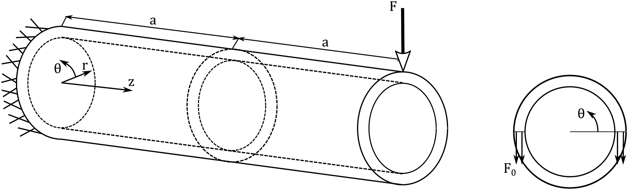
Cantilever tube under bending according to Sarvestani et al

Sarvestani et al. ⁵⁶ developed an approach for an orthotropic tube which is clamped on one end and loaded with the transverse force F on the other end using the cylindrical coordinate system (z, θ, r), see Figure 3. The general procedure has already been worked out in publications by Sarvestani and Sarvestani ⁵³ as well as Sarvestani and Sarvestani ⁵⁴ for plates.

Figure 3.

Cantilever tube model according to Sarvestani and Hojjati. ⁴⁵

It should be pointed out, that by comparsion with Lekhnitskii ² a permutated notation of material law and elastic constants is used. The first and third as well as the fourth and sixth entries of the stress and strain vectors are interchanged, whereby the rows and columns of the stiffness matrix are also adjusted. In contrast to the aforementioned models, the displacements, strains and stresses are discretized or interpolated over the radial component. Theoretical approaches are used for the other directions. 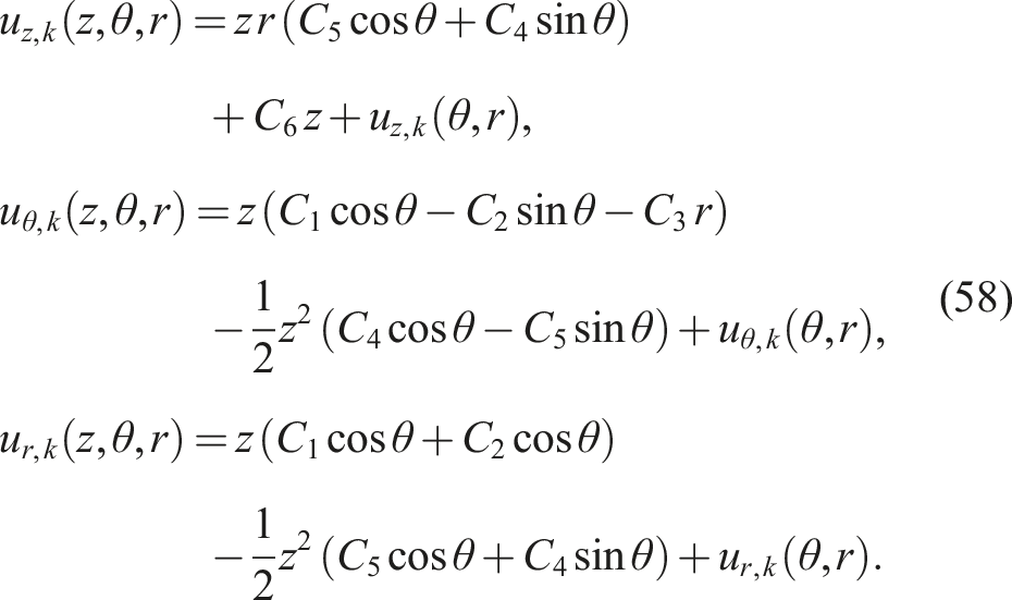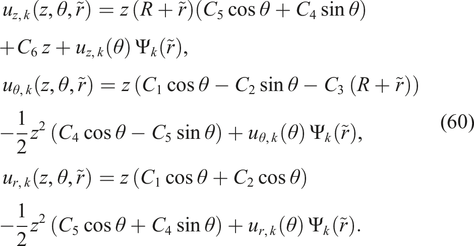⁵⁶ Although there is no real variation along the axial component z, since only different shear load values are used for different positions. Based on the strain-displacement relations (6) the following displacement field is obtained by integration and rearrangement

$\begin{array}{l}{u}_{z,k}\left(z,\theta ,r\right)=z\hspace{0.17em}r\hspace{0.17em}\left(C_5\hspace{0.17em}\cos \hspace{0.17em}\theta +C_4\hspace{0.17em}\sin \hspace{0.17em}\theta \right)\\ +C_6\hspace{0.17em}z+u_{z,k}\left(\theta ,r\right),\\ u_{\theta ,k}\left(z,\theta ,r\right)=z\hspace{0.17em}\left(C_1\hspace{0.17em}\cos \hspace{0.17em}\theta -C_2\hspace{0.17em}\sin \hspace{0.17em}\theta -C_3\hspace{0.17em}r\right)\\ -\frac{1}{2}\hspace{0.17em}{z}^2\hspace{0.17em}\left(C_4\hspace{0.17em}\cos \hspace{0.17em}\theta -C_5\hspace{0.17em}\sin \hspace{0.17em}\theta \right)+u_{\theta ,k}\left(\theta ,r\right),\\ u_{r,k}\left(z,\theta ,r\right)=z\hspace{0.17em}\left(C_1\hspace{0.17em}\cos \hspace{0.17em}\theta +C_2\hspace{0.17em}\cos \hspace{0.17em}\theta \right)\\ -\frac{1}{2}\hspace{0.17em}{z}^2\hspace{0.17em}\left(C_5\hspace{0.17em}\cos \hspace{0.17em}\theta +C_4\hspace{0.17em}\sin \hspace{0.17em}\theta \right)+u_{r,k}\left(\theta ,r\right).\end{array}$

(58)

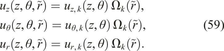
Moreover it is important that the unknown integration constants C₁-C₆ are the same for each layer k to ensure continuity of the displacements. In the so-called layerwise theory (LWT) with index k = 1 to N + 1 for the layer boundaries, the displacements of a general point are represented by

$\begin{array}{l}{u}_z\left(z,\theta ,\stackrel{\sim }{r}\right)=u_{z,k}\left(z,\theta \right)\hspace{0.17em}{\mathrm{\Omega }}_k\left(\stackrel{\sim }{r}\right),\\ u_{\theta }\left(z,\theta ,\stackrel{\sim }{r}\right)=u_{\theta ,k}\left(z,\theta \right)\hspace{0.17em}{\mathrm{\Omega }}_k\left(\stackrel{\sim }{r}\right),\\ u_r\left(z,\theta ,\stackrel{\sim }{r}\right)=u_{r,k}\left(z,\theta \right)\hspace{0.17em}{\mathrm{\Omega }}_k\left(\stackrel{\sim }{r}\right).\end{array}$

(59)

The parameter N represents the total number of numerical layers in the laminate, ${\mathrm{\Omega }}_k\left(\stackrel{\sim }{r}\right)$ the Lagrange interpolation formula to discretize along the coordinate $\stackrel{\sim }{r}$ of the k-th position and $\stackrel{\sim }{r}$ the coordinate of thickness direction originated in the center plane of the laminate. The local unknown functions u_z,k(z, θ), u_θ,k(z, θ) and u_r,k(z, θ), which are only dependent on two coordinates, are found by re-formulating the displacement field (58) using the principle of (59) to

$\begin{array}{l}{u}_{z,k}\left(z,\theta ,\stackrel{\sim }{r}\right)=z\hspace{0.17em}\left(R+\stackrel{\sim }{r}\right)\left(C_5\hspace{0.17em}\cos \hspace{0.17em}\theta +C_4\hspace{0.17em}\sin \hspace{0.17em}\theta \right)\\ +C_6\hspace{0.17em}z+u_{z,k}\left(\theta \right)\hspace{0.17em}{\mathrm{\Psi }}_k\left(\stackrel{\sim }{r}\right),\\ u_{\theta ,k}\left(z,\theta ,\stackrel{\sim }{r}\right)=z\hspace{0.17em}\left(C_1\hspace{0.17em}\cos \hspace{0.17em}\theta -C_2\hspace{0.17em}\sin \hspace{0.17em}\theta -C_3\hspace{0.17em}\left(R+\stackrel{\sim }{r}\right)\right)\\ -\frac{1}{2}\hspace{0.17em}{z}^2\hspace{0.17em}\left(C_4\hspace{0.17em}\cos \hspace{0.17em}\theta -C_5\hspace{0.17em}\sin \hspace{0.17em}\theta \right)+u_{\theta ,k}\left(\theta \right)\hspace{0.17em}{\mathrm{\Psi }}_k\left(\stackrel{\sim }{r}\right),\\ u_{r,k}\left(z,\theta ,\stackrel{\sim }{r}\right)=z\hspace{0.17em}\left(C_1\hspace{0.17em}\cos \hspace{0.17em}\theta +C_2\hspace{0.17em}\cos \hspace{0.17em}\theta \right)\\ -\frac{1}{2}\hspace{0.17em}{z}^2\hspace{0.17em}\left(C_5\hspace{0.17em}\cos \hspace{0.17em}\theta +C_4\hspace{0.17em}\sin \hspace{0.17em}\theta \right)+u_{r,k}\left(\theta \right)\hspace{0.17em}{\mathrm{\Psi }}_k\left(\stackrel{\sim }{r}\right).\end{array}$

(60)

Note that the relation $r=R+\stackrel{\sim }{r}$ with mean radius R of the tube was applied. The linear interpolation function ${\mathrm{\Psi }}_k\left(\stackrel{\sim }{r}\right)$ provides a continuous displacement behavior across the thickness, but the transverse strains remain discontinuous. By increasing the polynomial of the interpolation, the accuracy of the solution is increased. For linear interpolation, the equations are ⁵⁶

${\mathrm{\Psi }}_k(\stackrel{\sim }{r})=\{\begin{array}{ll}0& \stackrel{\sim }{r}\hspace{0.17em}\le \hspace{0.17em}{\stackrel{\sim }{r}}_{k-1},\\ {\mathrm{\Psi }}_{k-1}^2(\stackrel{\sim }{r})=\frac{1}{h(k-1)}\hspace{0.17em}(\stackrel{\sim }{r}-{\stackrel{\sim }{r}}_{k-1})& {\stackrel{\sim }{r}}_{k-1}\le \stackrel{\sim }{r}\hspace{0.17em}\le \hspace{0.17em}{\stackrel{\sim }{r}}_k,\\ {\mathrm{\Psi }}_k^1(\stackrel{\sim }{r})=\frac{1}{h_k}\hspace{0.17em}({\stackrel{\sim }{r}}_{k+1}-\stackrel{\sim }{r})& {\stackrel{\sim }{r}}_k\le \stackrel{\sim }{r}\hspace{0.17em}\le \hspace{0.17em}{\stackrel{\sim }{r}}_{k+1},\\ 0& \stackrel{\sim }{r}\ge {\stackrel{\sim }{r}}_{k+1}.\end{array}$

(61)

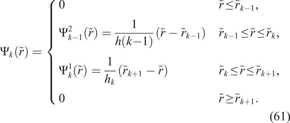
The parameter h _k corresponds to the layer thickness of the k-th position and ${\mathrm{\Psi }}_k^1\left(\stackrel{\sim }{r}\right)$ and ${\mathrm{\Psi }}_{k-1}^2\left(\stackrel{\sim }{r}\right)$ to local linear Lagrange interpolations. By using equation (60) with the strain-displacement relations (6), the strains can be expressed in dependence of the integration constants, the global lagrange interpolation and the unknown displacements u_z,k(θ), u_θ,k(θ) and u_r,k(θ) as functions only of hoop direction θ. Subsequently, the equilibrium equations are established by employing the strains to the principle of minimum potential energy. This results in an equation system with 3(N + 1) local equilibrium equations and unknown local displacements. In addition, the unknown displacements and constants C₁-C₆ can be represented as functions of the stresses and the given shear load F₀, which is assumed to be uniformly distributed over the radius, see Figure 3.

Finally the system of governing equations for the displacements is obtained using the global constitutive law in monotropic form and is solved by the use of boundary conditions. For model verification, the axial stress was compared with the model according to Lekhnitskii ² and showed good agreement. An increase of fictious layers, by additionally dividing the physical layers in the analysis, showed an approximation of the stresses in thickness direction in comparison to a finite element (FE) calculation. A good agreement was also found to experimental studies regarding three-point bending tests on pipes. Advantages of using the LWT for the cylindrical, orthotropic tube are simpler input values compared to FE calculations and a more accurate representation of the stresses and deformations in thickness direction compared to other tube models.

Curved tube under bending according to Sarvestani et al

Furthermore, a new displacement-based model of an orthotropic, curved tube with a single layer was developed by Sarvestani et al. ⁵⁷ for pure bending using the toroidal elasticity and the method of successive approximation. The toroidal elasticity (TE) is a known three-dimensional approach for the static analysis of thick-walled, curved tubes and was developed i. a. by the authors Lang ⁶⁰ as well as Zhu and Redekop. ⁶¹ In contrast to cylindrical approaches of straight pipes, the longitudinal axis is represented by an axis of rotation Φ instead of a cartesian coordinate z, see Figure 4.

Figure 4.

Curved tube according to Sarvestani et al. ⁵⁷

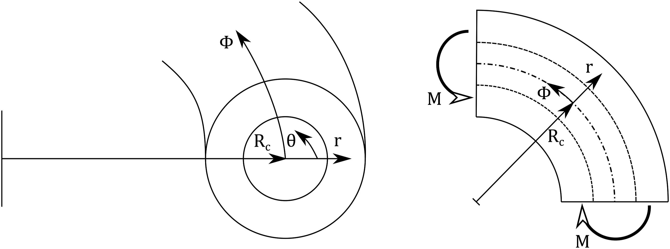
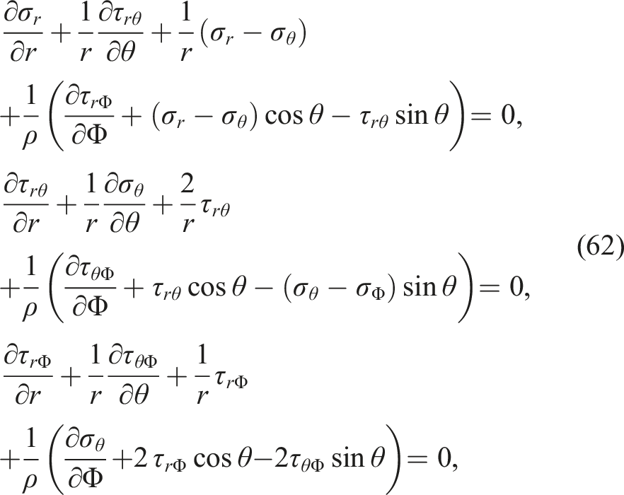
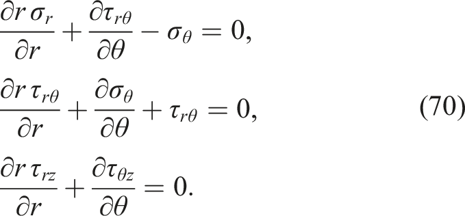
The toroidal equilibrium equations can be established using this coordinate system according to Sarvestani and Gorjipoor ⁵⁵ with ρ = R _c + r cos θ to

$\begin{array}{ll}& \frac{\partial {\sigma }_r}{\partial r}+\frac{1}{r}\hspace{0.17em}\frac{\partial {\tau }_{r\theta }}{\partial \theta }+\frac{1}{r}\hspace{0.17em}\left({\sigma }_r-{\sigma }_{\theta }\right)\\ & +\frac{1}{\rho }\hspace{0.17em}\left(\frac{\partial {\tau }_{r\mathrm{\Phi }}}{\partial \mathrm{\Phi }}+\left({\sigma }_r-{\sigma }_{\theta }\right)\hspace{0.17em}\cos \hspace{0.17em}\theta -{\tau }_{r\theta }\hspace{0.17em}\sin \hspace{0.17em}\theta \right)=0,\\ & \frac{\partial {\tau }_{r\theta }}{\partial r}+\frac{1}{r}\hspace{0.17em}\frac{\partial {\sigma }_{\theta }}{\partial \theta }+\frac{2}{r}\hspace{0.17em}{\tau }_{r\theta }\\ & +\frac{1}{\rho }\hspace{0.17em}\left(\frac{\partial {\tau }_{\theta \mathrm{\Phi }}}{\partial \mathrm{\Phi }}+{\tau }_{r\theta }\hspace{0.17em}\cos \hspace{0.17em}\theta -\left({\sigma }_{\theta }-{\sigma }_{\mathrm{\Phi }}\right)\hspace{0.17em}\sin \hspace{0.17em}\theta \right)=0,\\ & \frac{\partial {\tau }_{r\mathrm{\Phi }}}{\partial r}+\frac{1}{r}\hspace{0.17em}\frac{\partial {\tau }_{\theta \mathrm{\Phi }}}{\partial \theta }+\frac{1}{r}\hspace{0.17em}{\tau }_{r\mathrm{\Phi }}\\ & +\frac{1}{\rho }\hspace{0.17em}\left(\frac{\partial {\sigma }_{\theta }}{\partial \mathrm{\Phi }}+2\hspace{0.17em}{\tau }_{r\mathrm{\Phi }}\hspace{0.17em}\cos \hspace{0.17em}\theta -2{\tau }_{\theta \mathrm{\Phi }}\hspace{0.17em}\sin \hspace{0.17em}\theta \right)=0,\end{array}$

(62)

The strain-displacement relations are

${\epsilon }_r=\frac{\partial u_r}{\partial r},$

(63a)

${\epsilon }_{\theta }=\frac{u_r}{r}+\frac{1}{r}\hspace{0.17em}\frac{\partial u_{\theta }}{\partial \theta },$

(63b)

${\epsilon }_{\mathrm{\Phi }}=\frac{1}{\rho }\hspace{0.17em}\left(u_r\hspace{0.17em}\cos \hspace{0.17em}\theta -u_{\theta }\hspace{0.17em}\sin \hspace{0.17em}\theta +\frac{\partial u_{\mathrm{\Phi }}}{\partial \mathrm{\Phi }}\right),$

(63c)

${\gamma }_{r\theta }=\frac{1}{2}\hspace{0.17em}\left(\frac{1}{r}\hspace{0.17em}\frac{\partial u_r}{\partial \theta }+\frac{\partial u_{\theta }}{\partial r}-\frac{u_{\theta }}{r}\right),$

(63d)

${\gamma }_{r\mathrm{\Phi }}=\frac{1}{2}\hspace{0.17em}\left(\frac{\partial u_{\mathrm{\Phi }}}{\partial r}+\frac{1}{\rho }\hspace{0.17em}\frac{\partial u_r}{\partial \mathrm{\Phi }}-\frac{u_{\mathrm{\Phi }}}{\rho }\hspace{0.17em}\cos \hspace{0.17em}\theta \right),$

(63e)

${\gamma }_{\theta \mathrm{\Phi }}=\frac{1}{2}\hspace{0.17em}(\frac{1}{r}\hspace{0.17em}\frac{\partial u_{\mathrm{\Phi }}}{\partial \theta }+\frac{1}{\rho }\hspace{0.17em}\frac{\partial u_{\theta }}{\partial \mathrm{\Phi }}+\frac{u_{\mathrm{\Phi }}}{\rho }\hspace{0.17em}\sin \hspace{0.17em}\theta ).$

(63f)

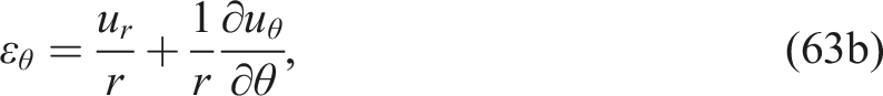
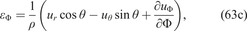
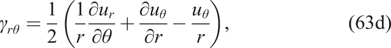
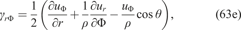
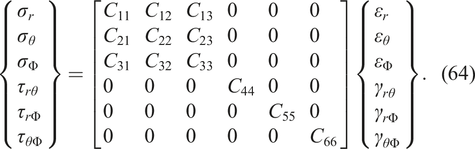
In contrast to the stress-based models, the material law is used in stiffness formulation according to Herakovich ⁶² for orthotropy. With permutation of the fourth and sixth row as well as column towards Lekhnitskii, ² it results in

$\left\{\begin{array}{l}{\sigma }_r\\ {\sigma }_{\theta }\\ {\sigma }_{\mathrm{\Phi }}\\ {\tau }_{r\theta }\\ {\tau }_{r\mathrm{\Phi }}\\ {\tau }_{\theta \mathrm{\Phi }}\end{array}\right\}=\left[\begin{array}{llllll}{C}_{11}& C_{12}& C_{13}& 0& 0& 0\\ C_{21}& C_{22}& C_{23}& 0& 0& 0\\ C_{31}& C_{32}& C_{33}& 0& 0& 0\\ 0& 0& 0& C_{44}& 0& 0\\ 0& 0& 0& 0& C_{55}& 0\\ 0& 0& 0& 0& 0& C_{66}\end{array}\right]\left\{\begin{array}{l}{\epsilon }_r\\ {\epsilon }_{\theta }\\ {\epsilon }_{\mathrm{\Phi }}\\ {\gamma }_{r\theta }\\ {\gamma }_{r\mathrm{\Phi }}\\ {\gamma }_{\theta \mathrm{\Phi }}\end{array}\right\}.$

(64)

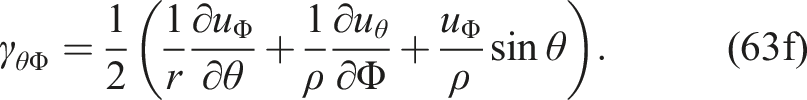
From the connection of the equilibrium equation (62) and the stress-displacement relations, again obtained from the strain-displacement relations (63a-63f) and the constitutive law (64), the system of descriptive Navier equations of the toroidal coordinate system is obtained as

$\begin{array}{l}{\left(\frac{1}{\rho }\right)}^0\hspace{0.17em}{U}_r+{\left(\frac{1}{\rho }\right)}^1\hspace{0.17em}{\overline{U}}_r+{\left(\frac{1}{\rho }\right)}^2\hspace{0.17em}{\widehat{U}}_r=0,\\ {\left(\frac{1}{\rho }\right)}^0\hspace{0.17em}{U}_{\theta }+{\left(\frac{1}{\rho }\right)}^1\hspace{0.17em}{\overline{U}}_{\theta }+{\left(\frac{1}{\rho }\right)}^2\hspace{0.17em}{\widehat{U}}_{\theta }=0,\\ {\left(\frac{1}{\rho }\right)}^0\hspace{0.17em}{U}_{\mathrm{\Phi }}+{\left(\frac{1}{\rho }\right)}^1\hspace{0.17em}{\overline{U}}_{\mathrm{\Phi }}+{\left(\frac{1}{\rho }\right)}^2\hspace{0.17em}{\widehat{U}}_{\mathrm{\Phi }}=0.\end{array}$

(65)

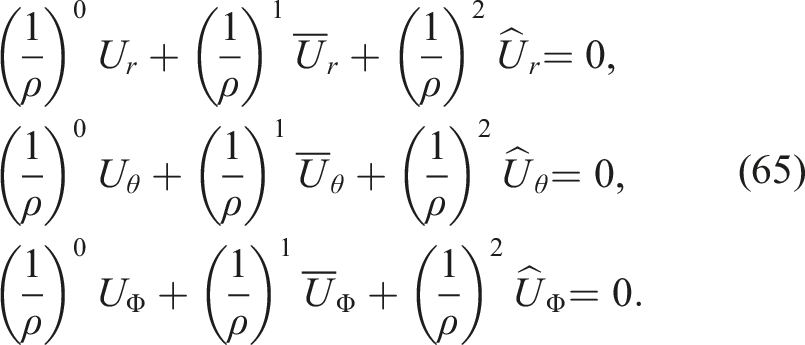
The geometric parameter ρ = R _c + r cos θ follows from the radius of the tube curvature R _c and the radial coordinate of the tube r. As can be seen, the displacements can be divided into a part independent of ρ, a linear-dependent, and a nonlinear-dependent part. The coefficients in (65) are

$\begin{array}{ll}{U}_{r,n}& =\frac{1}{2}\hspace{0.17em}{C}_{11}\hspace{0.17em}\frac{{\partial }^2{u}_{r,n}}{\partial r^2}+\frac{1}{2r}\hspace{0.17em}{C}_{11}\hspace{0.17em}\frac{\partial u_{r,n}}{\partial r}+\frac{C_{44}}{2r^2}\hspace{0.17em}\frac{{\partial }^2{u}_{r,n}}{\partial {\theta }^2}\\ & +\left(\frac{1}{2}\hspace{0.17em}{C}_{11}-C_{22}\right)\hspace{0.17em}\frac{u_{r,n}}{r^2}+\left(C_{12}-C_{22}\right)\hspace{0.17em}\frac{1}{r^2}\hspace{0.17em}\frac{{\partial }^2{u}_{\theta ,n}}{\partial \theta }\\ & +\frac{\partial }{\partial r}\hspace{0.17em}(\frac{1}{2}\hspace{0.17em}{C}_{11}\hspace{0.17em}\frac{u_{r,n}}{r}+\frac{1}{r}\left(\frac{C_{44}}{2}+C_{12}\right)\hspace{0.17em}\frac{\partial u_{\theta ,n}}{\partial \theta }\\ & +\frac{1}{2}\hspace{0.17em}{C}_{11}\hspace{0.17em}\frac{\partial u_{r,n}}{\partial r}),\end{array}$

(66a)

$\begin{array}{ll}{\overline{U}}_{r,n}& =\cos \hspace{0.17em}\theta \hspace{0.17em}\frac{\partial u_{r,n}}{\partial r}\hspace{0.17em}\left(C_{11}-C_{13}\right)-\hspace{0.17em}\sin \hspace{0.17em}\theta \hspace{0.17em}\frac{\partial u_{\theta ,n}}{\partial r}\hspace{0.17em}\frac{C_{44}}{2}\\ & -\hspace{0.17em}\sin \hspace{0.17em}\theta \hspace{0.17em}\frac{C_{44}}{2}\hspace{0.17em}\left(\frac{1}{r}\hspace{0.17em}\frac{\partial u_{r,n}}{\partial \theta }-\frac{u_{\theta ,n}}{r}\right)\\ & +\cos \hspace{0.17em}\theta \hspace{0.17em}\left(C_{12}-C_{23}\right)\left(\frac{1}{r}\hspace{0.17em}\frac{\partial u_{\theta ,n}}{\partial \theta }+\frac{u_{r,n}}{r}\right)\\ & +\frac{\partial }{\partial r}\hspace{0.17em}(\frac{C_{55}}{2}\hspace{0.17em}\frac{\partial u_{\mathrm{\Phi },n}}{\partial \mathrm{\Phi }}\\ & +C_{13}\hspace{0.17em}\left(u_{r,n}\hspace{0.17em}\cos \hspace{0.17em}\theta -u_{\theta ,n}\hspace{0.17em}\sin \hspace{0.17em}\theta +\frac{\partial u_{\mathrm{\Phi },n}}{\partial \mathrm{\Phi }}\right))\\ & +\frac{1}{r}\left(C_{13}-C_{23}\right)\left(u_{r,n}\hspace{0.17em}cos\hspace{0.17em}\theta -u_{\theta ,n}\hspace{0.17em}sin\hspace{0.17em}\theta +\frac{\partial u_{\mathrm{\Phi },n}}{\partial \mathrm{\Phi }}\right)\end{array}$

(66b)

$\begin{array}{ll}{\widehat{U}}_{r,n}& =\frac{C_{55}}{2}\hspace{0.17em}\frac{{\partial }^2{u}_{r,n}}{\partial {\mathrm{\Phi }}^2}-\frac{C_{55}}{2}\hspace{0.17em}\cos \hspace{0.17em}\theta \hspace{0.17em}\frac{\partial u_{\mathrm{\Phi },n}}{\partial \mathrm{\Phi }}\\ & -C_{33}\hspace{0.17em}\cos \hspace{0.17em}\theta \hspace{0.17em}\left(u_{r,n}\hspace{0.17em}\cos \hspace{0.17em}\theta -u_{\theta ,n}\hspace{0.17em}\sin \hspace{0.17em}\theta +\frac{\partial u_{\mathrm{\Phi },n}}{\partial \mathrm{\Phi }}\right),\end{array}$

(66c)

$\begin{array}{ll}{U}_{\theta ,n}& =\frac{C_{44}}{2}\hspace{0.17em}\frac{{\partial }^2{u}_{\theta ,n}}{\partial r^2}+\frac{1}{2r}\hspace{0.17em}{C}_{44}\hspace{0.17em}\frac{\partial u_{\theta ,n}}{\partial r}+\frac{C_{22}}{2r^2}\hspace{0.17em}\frac{{\partial }^2{u}_{\theta ,n}}{\partial {\theta }^2}\\ & -\frac{1}{2}\hspace{0.17em}{C}_{44}\hspace{0.17em}\frac{u_{\theta ,n}}{r^2}+\frac{1}{2}\hspace{0.17em}{C}_{44}\hspace{0.17em}\frac{1}{r^2}\hspace{0.17em}\frac{{\partial }^2{u}_{r,n}}{\partial \theta }\\ & +\frac{1}{r}\hspace{0.17em}\frac{\partial }{\partial \theta }\hspace{0.17em}(C_{22}\hspace{0.17em}\frac{u_{r,n}}{r}+\left(\frac{C_{44}}{2}+C_{12}\right)\hspace{0.17em}\frac{\partial u_{r,n}}{\partial r}\\ & +\frac{1}{2r}\hspace{0.17em}{C}_{22}\hspace{0.17em}\frac{\partial u_{\theta ,n}}{\partial \theta }),\end{array}$

(66d)

$\begin{array}{ll}{\overline{U}}_{\theta ,n}& =\cos \hspace{0.17em}\theta \hspace{0.17em}\frac{C_{44}}{2}\hspace{0.17em}\frac{\partial u_{\theta ,n}}{\partial r}-\hspace{0.17em}\sin \hspace{0.17em}\theta \hspace{0.17em}\left(C_{12}-C_{13}\right)\hspace{0.17em}\frac{\partial u_{r,n}}{\partial r}\\ & -\hspace{0.17em}\sin \hspace{0.17em}\theta \hspace{0.17em}\left(C_{22}-C_{23}\right)\cdot \left(\frac{1}{r}\hspace{0.17em}\frac{\partial u_{\theta ,n}}{\partial \theta }+\frac{u_{r,n}}{r}\right)\\ & +\cos \hspace{0.17em}\theta \hspace{0.17em}\frac{C_{44}}{2}\left(\frac{1}{r}\hspace{0.17em}\frac{\partial u_{r,n}}{\partial \theta }-\frac{u_{\theta ,n}}{r}\right)+\frac{1}{r}\hspace{0.17em}\frac{\partial }{\partial \theta }\hspace{0.17em}(\frac{C_{66}}{2}\hspace{0.17em}\frac{\partial u_{\mathrm{\Phi },n}}{\partial \mathrm{\Phi }}\\ & +C_{23}\hspace{0.17em}\left(u_{r,n}\hspace{0.17em}\cos \hspace{0.17em}\theta -u_{\theta ,n}\hspace{0.17em}\sin \hspace{0.17em}\theta +\frac{\partial u_{\mathrm{\Phi },n}}{\partial \mathrm{\Phi }}\right)),\end{array}$

(66e)

$\begin{array}{ll}{\widehat{U}}_{\theta ,n}& =\frac{C_{66}}{2}\hspace{0.17em}\frac{{\partial }^2{u}_{\theta ,n}}{\partial {\mathrm{\Phi }}^2}+\frac{C_{66}}{2}\hspace{0.17em}\sin \hspace{0.17em}\theta \hspace{0.17em}\frac{\partial u_{\mathrm{\Phi },n}}{\partial \mathrm{\Phi }}\\ & -C_{33}\hspace{0.17em}\sin \hspace{0.17em}\theta \hspace{0.17em}\left(u_{r,n}\hspace{0.17em}\cos \hspace{0.17em}\theta -u_{\theta ,n}\hspace{0.17em}\sin \hspace{0.17em}\theta +\frac{\partial u_{\mathrm{\Phi },n}}{\partial \mathrm{\Phi }}\right),\end{array}$

(66f)

$\begin{array}{ll}{U}_{\mathrm{\Phi },n}& =\frac{1}{2}\hspace{0.17em}{C}_{55}\hspace{0.17em}\frac{{\partial }^2{u}_{\mathrm{\Phi },n}}{\partial r^2}+\frac{1}{2r}\hspace{0.17em}{C}_{55}\hspace{0.17em}\frac{\partial u_{\mathrm{\Phi },n}}{\partial r}+\frac{C_{66}}{2r^2}\hspace{0.17em}\frac{{\partial }^2{u}_{\mathrm{\Phi },n}}{\partial {\theta }^2},\end{array}$

(66g)

$\begin{array}{ll}{\overline{U}}_{\mathrm{\Phi },n}& =\cos \hspace{0.17em}\theta \hspace{0.17em}\frac{C_{55}}{2}\hspace{0.17em}\frac{\partial u_{\mathrm{\Phi },n}}{\partial r}-\frac{1}{r}\hspace{0.17em}\cos \hspace{0.17em}\theta \hspace{0.17em}\left(\frac{C_{55}}{2}-\frac{C_{66}}{2}\right)\hspace{0.17em}{u}_{\mathrm{\Phi },n}\\ & -\frac{1}{r}\hspace{0.17em}\sin \hspace{0.17em}\theta \hspace{0.17em}\frac{C_{66}}{2}\hspace{0.17em}\frac{\partial u_{\mathrm{\Phi },n}}{\partial \theta }+\frac{\partial }{\partial \mathrm{\Phi }}\hspace{0.17em}(\left(\frac{C_{55}}{2}+C_{13}\right)\hspace{0.17em}\frac{\partial u_{r,n}}{\partial r}\\ & +\frac{1}{r}\hspace{0.17em}\left(\frac{C_{66}}{2}+C_{23}\right)\hspace{0.17em}\frac{\partial u_{\theta ,n}}{\partial \theta }+\frac{1}{r}\hspace{0.17em}\left(\frac{C_{55}}{2}+C_{23}\right)\hspace{0.17em}{u}_{r,n}),\end{array}$

(66h)

$\begin{array}{ll}{\widehat{U}}_{\mathrm{\Phi },n}& =\frac{C_{33}}{2}\hspace{0.17em}\frac{{\partial }^2{u}_{\mathrm{\Phi },n}}{\partial {\mathrm{\Phi }}^2}+(C_{55}\hspace{0.17em}\left(\frac{1}{2}\hspace{0.17em}{\cos }^2\hspace{0.17em}\theta -\hspace{0.17em}\cos \hspace{0.17em}\theta \right)\\ & +C_{66}\hspace{0.17em}\left(\frac{1}{2}\hspace{0.17em}{\sin }^2\hspace{0.17em}\theta -\hspace{0.17em}\sin \hspace{0.17em}\theta \right))\hspace{0.17em}{u}_{\mathrm{\Phi },n}\\ & +\frac{\partial }{\partial \mathrm{\Phi }}\hspace{0.17em}(\left(C_{33}+\frac{C_{55}}{2}\right)\hspace{0.17em}{u}_{r,n}\hspace{0.17em}\cos \hspace{0.17em}\theta \\ & -\left(C_{33}+\frac{C_{55}}{2}\right)u_{\theta ,n}\hspace{0.17em}\sin \hspace{0.17em}\theta +\frac{C_{33}}{2}\hspace{0.17em}\frac{\partial u_{\mathrm{\Phi },n}}{\partial \mathrm{\Phi }}).\end{array}$

(66i)

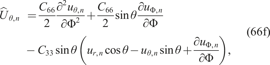
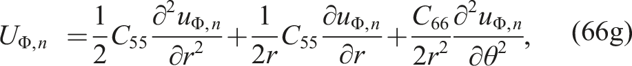
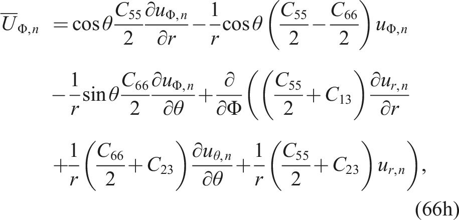
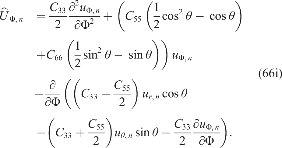
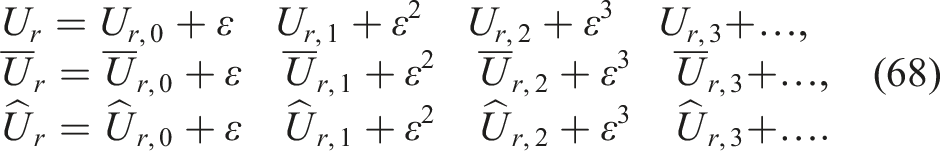
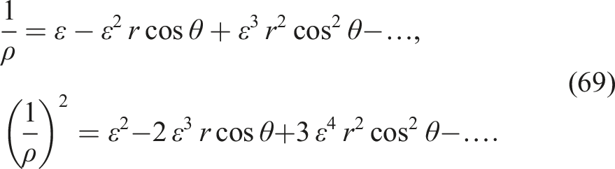
For equation (65) the subscripts n, which correspond to the order of the coefficients and displacements, vanish and for the later equation (68) they are used with n = 0-3. There is no exact solution for the Navier equations of toroidal elasticity, which is why the solution is approximated by the method of successive approximation. ⁵⁷ The displacement terms are obtained using the geometry parameter ɛ = r _i /R _c with

$\begin{array}{l}{u}_r=u_{r,0}+\epsilon \hspace{1em}{u}_{r,1}+{\epsilon }^2\hspace{1em}{u}_{r,2}+{\epsilon }^3{u}_{r,3}+\dots ,\\ u_{\theta }=u_{\theta ,0}+\epsilon \hspace{1em}{u}_{\theta ,1}+{\epsilon }^2\hspace{1em}{u}_{\theta ,2}+{\epsilon }^3\hspace{1em}{u}_{\theta ,3}+\dots ,\\ u_{\mathrm{\Phi }}=u_{\mathrm{\Phi },0}+\epsilon \hspace{1em}{u}_{\mathrm{\Phi },1}+{\epsilon }^2\hspace{1em}{u}_{\mathrm{\Phi },2}+{\epsilon }^3\hspace{1em}{u}_{\mathrm{\Phi },3}+\dots .\end{array}$

(67)

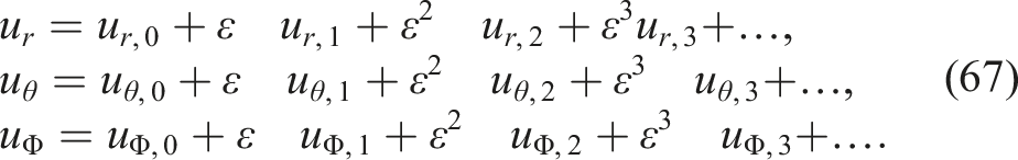
For the displacement parts of the Navier equations, the following equations are gained

$\begin{array}{l}{U}_r=U_{r,0}+\epsilon \hspace{1em}{U}_{r,1}+{\epsilon }^2\hspace{1em}{U}_{r,2}+{\epsilon }^3\hspace{1em}{U}_{r,3}+\dots ,\\ {\overline{U}}_r={\overline{U}}_{r,0}+\epsilon \hspace{1em}{\overline{U}}_{r,1}+{\epsilon }^2\hspace{1em}{\overline{U}}_{r,2}+{\epsilon }^3\hspace{1em}{\overline{U}}_{r,3}+\dots ,\\ {\widehat{U}}_r={\widehat{U}}_{r,0}+\epsilon \hspace{1em}{\widehat{U}}_{r,1}+{\epsilon }^2\hspace{1em}{\widehat{U}}_{r,2}+{\epsilon }^3\hspace{1em}{\widehat{U}}_{r,3}+\dots .\end{array}$

(68)

Analogously, the equations for U _θ , ${\overline{U}}_{\theta }$ , ${\widehat{U}}_{\theta }$ and U_Φ, ${\overline{U}}_{\mathrm{\Phi }}$ , ${\widehat{U}}_{\mathrm{\Phi }}$ are obtained. A Taylor series approach is used for the terms with ρ in the form

$\begin{array}{l}\frac{1}{\rho }=\epsilon -{\epsilon }^2\hspace{0.17em}r\hspace{0.17em}\cos \hspace{0.17em}\theta +{\epsilon }^3\hspace{0.17em}{r}^2\hspace{0.17em}{\cos }^2\hspace{0.17em}\theta -\dots ,\\ {\left(\frac{1}{\rho }\right)}^2={\epsilon }^2-2\hspace{0.17em}{\epsilon }^3\hspace{0.17em}r\hspace{0.17em}\cos \hspace{0.17em}\theta +3\hspace{0.17em}{\epsilon }^4\hspace{0.17em}{r}^2\hspace{0.17em}{\cos }^2\hspace{0.17em}\theta -\dots .\end{array}$

(69)

After the equations (68) and (69) are inserted into the equation system (65), the terms of the different orders of ɛ are ordered and their coefficients are set to zero. This results in equation systems for the displacements of the respective order, which must be solved. The equation system of zeroth order only consists of a homogeneous solution, while the equation systems of higher order also have a particulate solution. Both are found using initial functions in trigonometric form. The general solution is obtained by considering all single solutions in the general displacement equations. For smaller geometric ratios ɛ the first terms of low order already provide a good approximation of the exact solution. In their paper, Sarvestani et al. ⁵⁷ verify their model by matching the curved isotropic case to literature values, the curved orthotropic case to FE simulations and the straight orthotropic case to the calculation method of Lekhnitskii. ² The straight tube is approximated with a ratio of R _c /r _i = 75 and all verifications showed good agreement.

In Sarvestani and Hojjati, ⁴⁵ the displacement-based model of Sarvestani et al. ⁵⁷ is extended to a multi-layer composite using a layerwise theory and Lagrange interpolation functions in a similar way as described in section Cantilever tube under bending according to Sarvestani et al. for a straight cantilever tube.

State-Space approaches

In the state-space approach the governing system of equations of a continuum is formulated in matrix form and in dependence of a state vector. Even though the state vector may only consist of stresses or displacements, the common approach is to use a combination of both. It is further appropriate to use state variables, that are needed for continuity conditions over the radial direction.

Axisymmetric tube formulations

In the research group surrounding Fan, Sheng and Ye, numerous publications were developed to the state-space approach of thick-walled plates, shells or cylindrical shells (tubes), see i. a. Fan and Sheng ⁶³ and Sheng and Le. ⁶⁴ In Fan and Ding, ⁶⁵ a pipe or closed cylindrical shell clamped on both sides under internal pressure is analytically described. However, this model applies only to axisymmetric loads, no changes over θ and an approximation of the thickness direction r using the method of successive approximation with N thin-walled subcylinders. The exact solution is thus approximated, but small errors remain. Compared to the FE solution, however, the stresses and displacements of the state vector can be displayed continuously over the laminate thickness. ⁶⁵ The method of successive approximation was introduced for isotropic shells by Soldatos and Hadjigeorgiou ⁶⁶ and has been extended to orthotropic shells by Hawkes and Soldatos. ⁶⁷ Since the differential equation system has variable coefficents for these models by virtue of the term $1+\stackrel{\sim }{r}/R^{-1}$ , depending on the ratio of thickness coordinate $\stackrel{\sim }{r}$ to mean radius R, a power series expansion for this term is used in the form $1+\stackrel{\sim }{r}/R^{-1}=1-\stackrel{\sim }{r}/R+{\stackrel{\sim }{r}}^2/R^2$ to obtain constant coefficients. ⁶⁶ If the number of sublayers N tends to infinity, the thickness of each subcylinder approaches zero and the usage of the power series becomes more insignificant. ⁶⁷ Many of the models are suitable for static as well as dynamic investigations due to the formulation as an eigenvalue problem.

Sheng and Ye ⁶⁸ formulated a three-dimensional, semi-analytic model of a multi-layer tube under axisymmetric bending. In this case, the tube is clamped on both sides, as a result of which the displacements become zero, and is stressed over the entire length and circumferential direction with a uniform internal or external pressure. Due to the coupling between longitudinal and torsional deformation, the 3D analysis is used only for axisymmetric loads and the stresses do not change over the circumferential component θ. ⁶⁸ The displacements u _r , u _θ , u _z and the stresses τ _rz , τ _rθ , σ _r in thickness direction are used as state variables. First, the state equation for a thin-walled single-layer tube is set up using a displacement approach and a Fourier series approximation in axial direction. Thinness is here defined by a ratio of wall thickness to radius smaller than 0.01. ⁶⁸ The expansion to thick-walled, multi-layered pipes is achieved by a radial subdivision into N sub-tubes, each of which satisfies thinness and adds fictive interphases within the layers to the real interphases at the layer boundaries. The system can be solved via continuity conditions of the state vector for all interphases and boundary conditions at the uniformly stressed or fixed envelope surfaces. The remaining three stresses can be discontinous. Analytical examples show the displacement and stress course over the axial and radial component. The basis for the approach by Sheng and Ye ⁶⁸ is the use of a recursive formulation of the state equations and continuity conditions at the interphases introduced in Fan and Ye ⁶⁹ for thick-walled plates. By this notation, the order of the state equation of the entire laminate is independent of the number of sub-layers N since the interphase boundary conditions must not be integrated into the global equation. ⁶⁴

In Ye and Soldatos ⁷⁰ the recursive algorithm according to Fan and Ye ⁶⁹ is also used in combination with the division into N sub-tubes for the fulfillment of thinness in each fictitious layer. As the continuum used, an open as well as a closed cylindrical shell is described under general surface traction. The respective loads are usually applied in dynamic form as harmonics via Fourier series. The core of the paper is the convergence consideration of the displacement and stress profiles with increasing number of sub-layers N. It is expected that as the number increases, the approximate solution approaches the exact solution of three-dimensional elasticity. It was found that for more complex loads, such as bending, convergence occurs much later, even though the examples explained in Ye and Soldatos ⁷⁰ only represent internal and external pressure considerations. Ye and Soldatos ⁷⁰ validate their approach by comparison with other, exact models of cylindrical shells under radial pressure.

Tube under bending according to Tarn and Wang

In addition to axisymmetric loads, Tarn and Wang ³⁰ are treating the load case of pure bending in their tube model formulated in state-space. As in most pipe models, the loads do not vary along the axial coordinate and the bending load is not coupled to the other loads. An innovation is the formulation of the state vector as a function of r. Thus, the system matrix of the state equation becomes independent of r and a solution by ordinary matrix algebra is made possible. The state vector {R} becomes ${\left\{u_r,u_{\theta },u_z,r {\sigma }_r,r {\tau }_{r\theta },r {\tau }_{rz}\right\}}^T$ . The equilibrium conditions (5), as also used in Lekhnitskii, ² are obtained by reformulation with the multiplication of r and ∂/∂z = 0 to

$\begin{array}{l}\frac{\partial r\hspace{0.17em}{\sigma }_r}{\partial r}+\frac{\partial {\tau }_{r\theta }}{\partial \theta }-{\sigma }_{\theta }=0,\\ \frac{\partial r\hspace{0.17em}{\tau }_{r\theta }}{\partial r}+\frac{\partial {\sigma }_{\theta }}{\partial \theta }+{\tau }_{r\theta }=0,\\ \frac{\partial r\hspace{0.17em}{\tau }_{rz}}{\partial r}+\frac{\partial {\tau }_{\theta z}}{\partial \theta }=0.\end{array}$

(70)

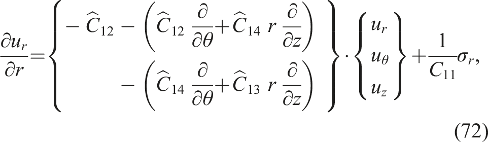
Using the monotropic material law in stiffness formulation and strain-displacement relations (6), the material law of each layer k can be expressed by

$\begin{array}{l}{\left\{\begin{array}{l}{\sigma }_r\\ {\sigma }_{\theta }\\ {\sigma }_z\\ {\tau }_{\theta z}\\ {\tau }_{rz}\\ {\tau }_{r\theta }\end{array}\right\}}_k={\left[\begin{array}{llllll}{C}_{11}& C_{12}& C_{13}& C_{14}& 0& 0\\ C_{21}& C_{22}& C_{23}& C_{24}& 0& 0\\ C_{31}& C_{32}& C_{33}& C_{34}& 0& 0\\ C_{41}& C_{42}& C_{43}& C_{44}& 0& 0\\ 0& 0& 0& 0& C_{55}& C_{56}\\ 0& 0& 0& 0& C_{65}& C_{66}\end{array}\right]}_k\cdot \\ \cdot {\left\{\begin{array}{l}\frac{\partial u_r}{\partial r}\\ \frac{1}{r}\hspace{1em}\frac{\partial u_{\theta }}{\partial \theta }+\frac{u_r}{r}\\ \frac{\partial u_z}{\partial z}\\ \frac{\partial u_{\theta }}{\partial z}+\frac{1}{r}\hspace{1em}\frac{\partial u_z}{\partial \theta }\\ \frac{\partial u_z}{\partial r}+\frac{\partial u_r}{\partial z}\\ \frac{1}{r}\hspace{1em}\frac{\partial u_r}{\partial \theta }+\frac{\partial u_{\theta }}{\partial r}-\frac{u_{\theta }}{r}\end{array}\right\}}_k.\end{array}$

(71)

Note again the notation sequence, which corresponds without permutation to the notation of Lekhnitskii. ² From the first equation of (71) follows

$\begin{array}{ll}\frac{\partial u_r}{\partial r}=& \left\{\begin{array}{lll}-{\widehat{C}}_{12}& -\left({\widehat{C}}_{12}\hspace{1em}\frac{\partial }{\partial \theta }+{\widehat{C}}_{14}\hspace{1em}r\hspace{1em}\frac{\partial }{\partial z}\right)& -\left({\widehat{C}}_{14}\hspace{1em}\frac{\partial }{\partial \theta }+{\widehat{C}}_{13}\hspace{1em}r\hspace{1em}\frac{\partial }{\partial z}\right)\end{array}\right\}\\ & \cdot \left\{\begin{array}{l}{u}_r\\ u_{\theta }\\ u_z\end{array}\right\}+\frac{1}{C_{11}}{\sigma }_r,\end{array}$

(72)

whereby for i, j = 1-4. With this equation (72) inserted into the second, third and fourth equations of (71), the stresses are expressed by

$\begin{array}{ll}{\sigma }_{\theta }=& \frac{1}{r}\left\{\begin{array}{lll}{Q}_{22}& Q_{22}\hspace{1em}\frac{\partial }{\partial \theta }+Q_{24}\hspace{1em}r\hspace{1em}\frac{\partial }{\partial z}& Q_{24}\hspace{1em}\frac{\partial }{\partial \theta }+Q_{23}\hspace{1em}r\hspace{1em}\frac{\partial }{\partial z}\end{array}\right\}\left\{\begin{array}{l}{u}_r\\ u_{\theta }\\ u_z\end{array}\right\}\\ & +{\widehat{C}}_{12}{\sigma }_r,\\ {\sigma }_z=& \frac{1}{r}\left\{\begin{array}{lll}{Q}_{23}& Q_{23}\hspace{1em}\frac{\partial }{\partial \theta }+Q_{34}\hspace{1em}r\hspace{1em}\frac{\partial }{\partial z}& Q_{34}\hspace{1em}\frac{\partial }{\partial \theta }+Q_{33}\hspace{1em}r\hspace{1em}\frac{\partial }{\partial z}\end{array}\right\}\left\{\begin{array}{l}{u}_r\\ u_{\theta }\\ u_z\end{array}\right\}\\ & +{\widehat{C}}_{13}{\sigma }_r,\\ {\tau }_{\theta z}=& \frac{1}{r}\left\{\begin{array}{lll}{Q}_{24}& Q_{24}\hspace{1em}\frac{\partial }{\partial \theta }+Q_{44}\hspace{1em}r\hspace{1em}\frac{\partial }{\partial z}& Q_{44}\hspace{1em}\frac{\partial }{\partial \theta }+Q_{34}\hspace{1em}r\hspace{1em}\frac{\partial }{\partial z}\end{array}\right\}\left\{\begin{array}{l}{u}_r\\ u_{\theta }\\ u_z\end{array}\right\}\\ & +{\widehat{C}}_{14}{\sigma }_r,\end{array}$

(73)

with reduced stiffnesses Q _ij = (C _ij − C_1i C_1j)/C₁₁ for i, j = 1-4. The fifth and sixth equation of (71) yield

$\frac{\partial }{\partial r}\left\{\begin{array}{l}{u}_{\theta }\\ u_z\end{array}\right\}=\frac{1}{r}\left\{\begin{array}{ll}-\frac{\partial }{\partial \theta }& 1\\ -r\hspace{1em}\frac{\partial }{\partial z}& 0\end{array}\right\}\left\{\begin{array}{l}{u}_r\\ u_{\theta }\end{array}\right\}+\left[\begin{array}{ll}{C}_{66}& C_{56}\\ C_{56}& C_{55}\end{array}\right]\left\{\begin{array}{l}{\tau }_{rz}\\ {\tau }_{r\theta }\end{array}\right\}.$

(74)

And equations (72) to (73) applied to the new equilibrium equation (70) provide

$\begin{array}{l}\frac{\partial }{\partial r}\hspace{1em}\left(r {\sigma }_r\right)=\frac{1}{r}\left\{\begin{array}{lll}{Q}_{22}& Q_{22} \frac{\partial }{\partial \theta }+Q_{24}\hspace{1em}r\hspace{1em}\frac{\partial }{\partial z}& Q_{24}\hspace{1em}\frac{\partial }{\partial \theta }+Q_{23}\hspace{1em}r\hspace{1em}\frac{\partial }{\partial z}\end{array}\right\}\\ \cdot \left\{\begin{array}{l}{u}_r\\ u_{\theta }\\ u_z\end{array}\right\}+{\hat{C}}_{12}{\sigma }_r-\frac{\partial }{\partial \theta }\hspace{1em}{\tau }_{r\theta },\\ \frac{\partial }{\partial r}\left(r {\tau }_{r\theta }\right)=-\frac{1}{r}\left\{\begin{array}{lll}{Q}_{22}& Q_{22} \frac{\partial }{\partial \theta }+Q_{24}\hspace{1em}r\hspace{1em}\frac{\partial }{\partial z}& Q_{24}\hspace{1em}\frac{\partial }{\partial \theta }+Q_{23}\hspace{1em}r\hspace{1em}\frac{\partial }{\partial z}\end{array}\right\}\\ \cdot \left\{\begin{array}{l}{u}_r\\ u_{\theta }\\ u_z\end{array}\right\}-{\hat{C}}_{12}\frac{\partial }{\partial \theta }\hspace{1em}{\sigma }_r-{\tau }_{r\theta },\\ \frac{\partial }{\partial r}\left(r {\tau }_{rz}\right)=-\frac{1}{r}\left\{\begin{array}{lll}{Q}_{24}& Q_{24} \frac{\partial }{\partial \theta }+Q_{44}\hspace{1em}r\hspace{1em}\frac{\partial }{\partial z}& Q_{44}\hspace{1em}\frac{\partial }{\partial \theta }+Q_{34}\hspace{1em}r\hspace{1em}\frac{\partial }{\partial z}\end{array}\right\}\\ \cdot \left\{\begin{array}{l}{u}_r\\ u_{\theta }\\ u_z\end{array}\right\}+{\hat{C}}_{14}\hspace{1em}\frac{\partial }{\partial \theta }\hspace{1em}{\sigma }_r.\end{array}$

(75)

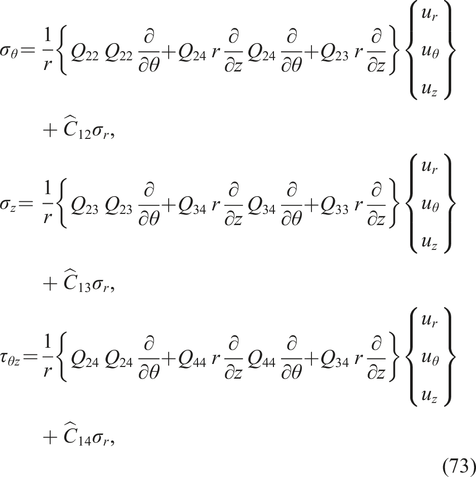
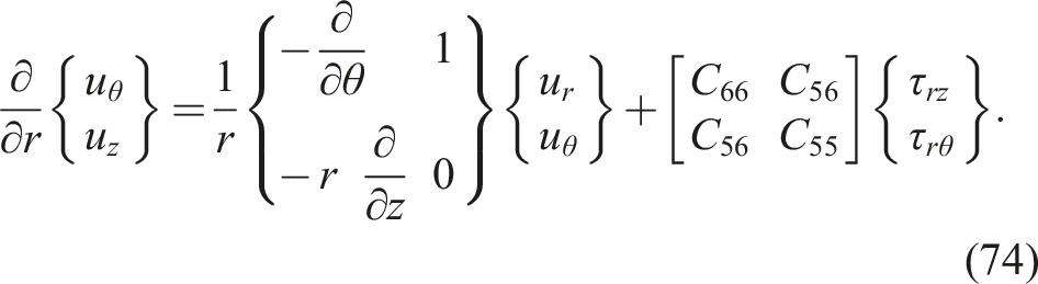
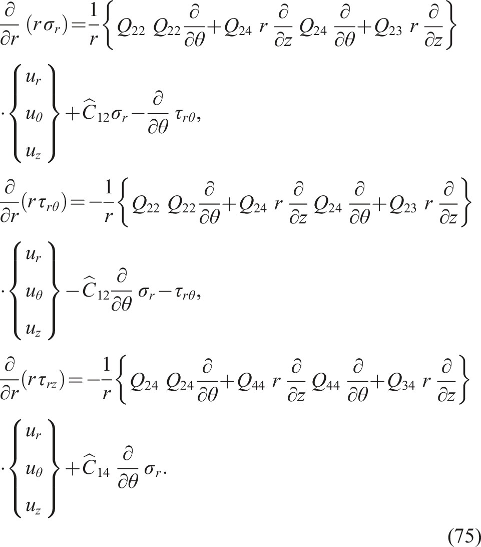
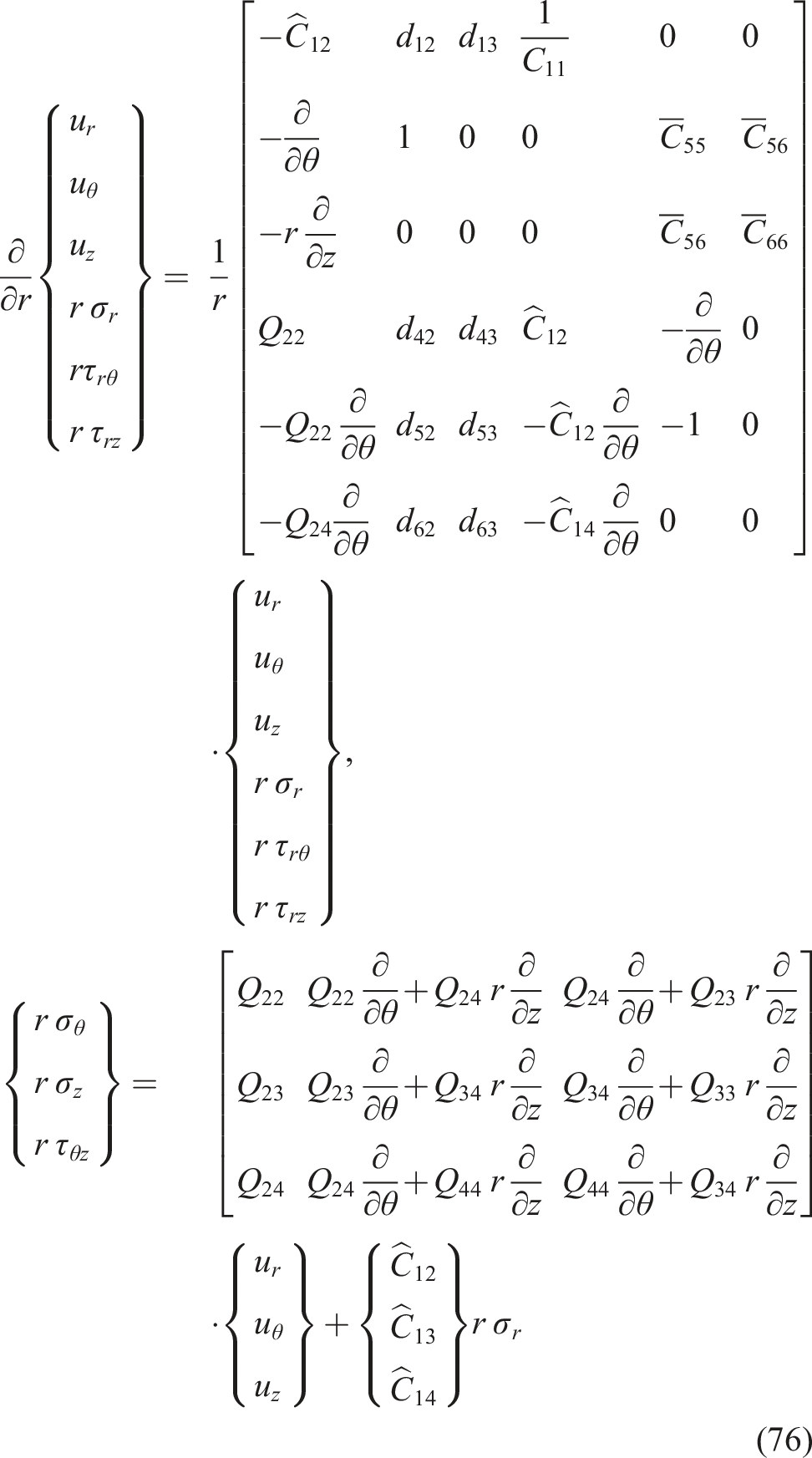
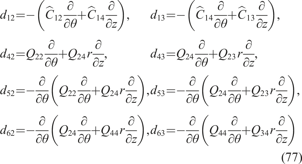
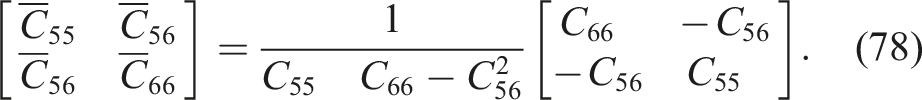
Finally, writing equations (72) to (75) in matrix form leads to the state equations in the form of equation (8) to

$\begin{array}{ll}\frac{\partial }{\partial r}\left\{\begin{array}{l}{u}_r\\ u_{\theta }\\ u_z\\ r {\sigma }_r\\ r{\tau }_{r\theta }\\ r {\tau }_{rz}\end{array}\right\}=& \frac{1}{r}\left[\begin{array}{llllll}-{\hat{C}}_{12}& d_{12}& d_{13}& \frac{1}{C_{11}}& 0& 0\\ -\frac{\partial }{\partial \theta }& 1& 0& 0& {\overline{C}}_{55}& {\overline{C}}_{56}\\ -r \frac{\partial }{\partial z}& 0& 0& 0& {\overline{C}}_{56}& {\overline{C}}_{66}\\ Q_{22}& d_{42}& d_{43}& {\hat{C}}_{12}& -\frac{\partial }{\partial \theta }& 0\\ -Q_{22} \frac{\partial }{\partial \theta }& d_{52}& d_{53}& -{\hat{C}}_{12} \frac{\partial }{\partial \theta }& -1& 0\\ -Q_{24}\frac{\partial }{\partial \theta }& d_{62}& d_{63}& -{\hat{C}}_{14} \frac{\partial }{\partial \theta }& 0& 0\end{array}\right]\\ & \cdot \left\{\begin{array}{l}{u}_r\\ u_{\theta }\\ u_z\\ r {\sigma }_r\\ r {\tau }_{r\theta }\\ r {\tau }_{rz}\end{array}\right\},\\ \left\{\begin{array}{l}r {\sigma }_{\theta }\\ r {\sigma }_z\\ r {\tau }_{\theta z}\end{array}\right\}=& \left[\begin{array}{lll}{Q}_{22}& Q_{22} \frac{\partial }{\partial \theta }+Q_{24} r \frac{\partial }{\partial z}& Q_{24} \frac{\partial }{\partial \theta }+Q_{23} r \frac{\partial }{\partial z}\\ Q_{23}& Q_{23} \frac{\partial }{\partial \theta }+Q_{34} r \frac{\partial }{\partial z}& Q_{34} \frac{\partial }{\partial \theta }+Q_{33} r \frac{\partial }{\partial z}\\ Q_{24}& Q_{24} \frac{\partial }{\partial \theta }+Q_{44} r \frac{\partial }{\partial z}& Q_{44} \frac{\partial }{\partial \theta }+Q_{34} r \frac{\partial }{\partial z}\end{array}\right]\\ & \cdot \left\{\begin{array}{l}{u}_r\\ u_{\theta }\\ u_z\end{array}\right\}+\left\{\begin{array}{l}{\hat{C}}_{12}\\ {\hat{C}}_{13}\\ {\hat{C}}_{14}\end{array}\right\}r {\sigma }_r\end{array}$

(76)

with

$\begin{array}{llll}{d}_{12}=-\left({\widehat{C}}_{12}\hspace{1em}\frac{\partial }{\partial \theta }+{\widehat{C}}_{14}\hspace{1em}\frac{\partial }{\partial z}\right),& d_{13}=-\left({\widehat{C}}_{14}\hspace{1em}\frac{\partial }{\partial \theta }+{\widehat{C}}_{13}\hspace{1em}\frac{\partial }{\partial z}\right),& & \\ d_{42}=Q_{22}\hspace{1em}\frac{\partial }{\partial \theta }+Q_{24}\hspace{1em}r\hspace{1em}\frac{\partial }{\partial z},& d_{43}=Q_{24}\hspace{1em}\frac{\partial }{\partial \theta }+Q_{23}\hspace{1em}r\hspace{1em}\frac{\partial }{\partial z},& & \\ d_{52}=-\frac{\partial }{\partial \theta }\hspace{1em}\left(Q_{22}\hspace{1em}\frac{\partial }{\partial \theta }+Q_{24}\hspace{1em}r\hspace{1em}\frac{\partial }{\partial z}\right),& d_{53}=-\frac{\partial }{\partial \theta }\hspace{1em}\left(Q_{24}\hspace{1em}\frac{\partial }{\partial \theta }+Q_{23}\hspace{1em}r\hspace{1em}\frac{\partial }{\partial z}\right),& & \\ d_{62}=-\frac{\partial }{\partial \theta }\hspace{1em}\left(Q_{24}\hspace{1em}\frac{\partial }{\partial \theta }+Q_{44}\hspace{1em}r\hspace{1em}\frac{\partial }{\partial z}\right),& d_{63}=-\frac{\partial }{\partial \theta }\hspace{1em}\left(Q_{44}\hspace{1em}\frac{\partial }{\partial \theta }+Q_{34}\hspace{1em}r\hspace{1em}\frac{\partial }{\partial z}\right)& & \end{array}$

(77)

and

$\left[\begin{array}{ll}{\overline{C}}_{55}& {\overline{C}}_{56}\\ {\overline{C}}_{56}& {\overline{C}}_{66}\end{array}\right]=\frac{1}{C_{55}\hspace{1em}{C}_{66}-C_{56}^2}\left[\begin{array}{ll}{C}_{66}& -C_{56}\\ -C_{56}& C_{55}\end{array}\right].$

(78)

After substituting the displacement field according to Lekhnitskii ² into the state equation (76), the solution is searched for using the following initial functions for the state vector

$\left\{\begin{array}{l}{u}_r\\ u_{\theta }\\ u_z\\ r\hspace{0.17em}{\sigma }_r\\ r\hspace{0.17em}{\tau }_{r\theta }\\ r\hspace{0.17em}{\tau }_{rz}\end{array}\right\}=\left\{\begin{array}{l}{U}_1\left(r\right)\\ V_1\left(r\right)\\ W_1\left(r\right)\\ X_1\left(r\right)\\ Y_1\left(r\right)\\ Z_1\left(r\right)\end{array}\right\}+\left\{\begin{array}{l}{U}_2\left(r\right)\hspace{0.17em}\cos \hspace{0.17em}\theta \\ V_2\left(r\right)\hspace{0.17em}\sin \hspace{0.17em}\theta \\ W_2\left(r\right)\hspace{0.17em}\sin \hspace{0.17em}\theta \\ X_2\left(r\right)\hspace{0.17em}\cos \hspace{0.17em}\theta \\ Y_2\left(r\right)\hspace{0.17em}\sin \hspace{0.17em}\theta \\ Z_2\left(r\right)\hspace{0.17em}\sin \hspace{0.17em}\theta \end{array}\right\}+\left\{\begin{array}{l}{U}_3\left(r\right)\hspace{0.17em}\sin \hspace{0.17em}\theta \\ V_3\left(r\right)\hspace{0.17em}\cos \hspace{0.17em}\theta \\ W_3\left(r\right)\hspace{0.17em}\cos \hspace{0.17em}\theta \\ X_3\left(r\right)\hspace{0.17em}\sin \hspace{0.17em}\theta \\ Y_3\left(r\right)\hspace{0.17em}\cos \hspace{0.17em}\theta \\ Z_3\left(r\right)\hspace{0.17em}\cos \hspace{0.17em}\theta \end{array}\right\}.$

(79)

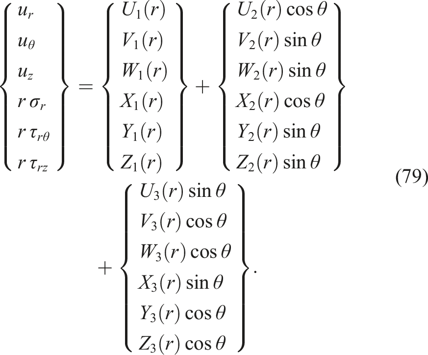
This results in three sets of uncoupled first-order differential equations separated into axisymmetric loads (index ’1’) and bending loads around x as well as y axes (indices ’2’ and ’3’), which have to be solved separately. The unknown coefficients U₁(r)-Z₃(r) are determined in the solution procedure. Thus a constant distribution over θ for axisymmetric and a trigonometric distribution for bending loads is given by the initial functions. The solution of the single systems is again achieved by the search for a homogeneous and particulate solution and the use of boundary conditions. For a multi-layer composite, the state equation for each layer k has to be solved, where continuity conditions of the state vector are used as additional boundary conditions.

Determination of an equivalent flexural stiffness

In addition to the elastic constants of the individual layers, many compliance-based models also provide an equivalent bending stiffness ⟨EI⟩. In general this equivalent stiffness is represented by the relationship between bending moments and curvatures, for example in the model of Jolicoeur and Cardou ⁴⁶ in section Multi-Layered tube according to Jolicoeur and Cardou, by

$\begin{array}{l}{M}_x=〈E\hspace{0.17em}I〉\hspace{0.17em}{\kappa }_x,\\ M_y=〈E\hspace{0.17em}I〉\hspace{0.17em}{\kappa }_y.\end{array}$

(80)

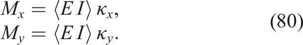
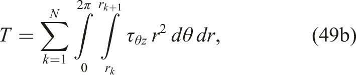
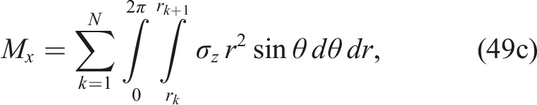
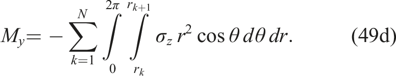
There is no coupling between M _x and κ _y or M _y and κ _x , which means that the curvatures only occur in the plane perpendicular to the bending load axis. ⁴⁶ Using the equation (49c) the moment M _x can be represented as a function of the stress σ _z . Considering that there are no axisymmetric loads, and thus ɛ, ϑ and the constants - $K_1^I$ - $K_2^I$ become zero, the equivalent bending stiffness follows from integration of the applied stresses and a reformulation of (80) to

$\begin{array}{ll}⟨E I⟩=& \sum _{n=0}^N\frac{\pi }{S_{33,n}}\hspace{1em}\{\sum _{i=1}^4{K}_{i,n}\hspace{1em}[S_{13,n}+S_{23,n}\hspace{1em}\left(m_{i,n}+1\right)\\ & -S_{34,n} g_{i,n} m_{i,n}]\frac{r_n^{m_{i,n}+2}-r_{n+1}^{m_{i,n}+2}}{m_{i,n}+2}\\ & +\left[{\mu }_{1,n}\hspace{1em}\left(S_{13,n}+3 S_{23,n}\right)-2 {\mu }_{2,n} S_{34,n}-1\right]\hspace{1em}\frac{r_n^4-r_{n+1}^4}{4}\}.\end{array}$

(81)

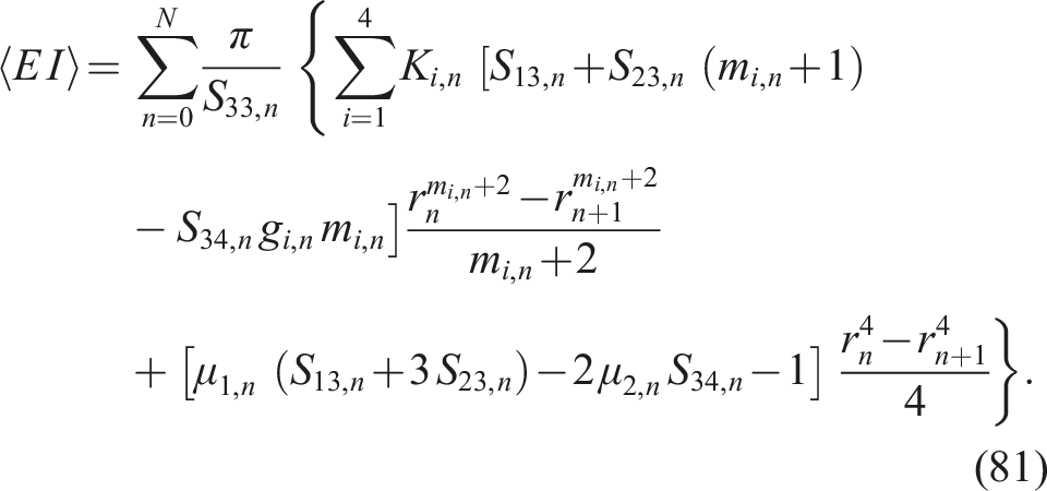
The abbreviations g_i,n, m_i,n and μ_1,n can be found from the equation (40) and C_i,n are known for each layer n after solving the model.

Geuchy Ahmad and Hoa ⁷¹ are comparing the approach for the equivalent bending stiffness of an anisotropic tube using the three-dimensional elasticity theory according to Jolicoeur and Cardou, ⁴⁶ see equation (81), with the classical approach from isotropic strength of materials and beam theory

$E\hspace{0.17em}{I}_{\text{circular} \text{ring}}=E \frac{\pi }{64}\left(D_a^4-D_i^4\right).$

(82)

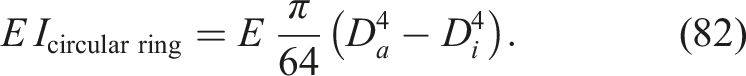
The surface moment of inertia I is directly applied for a circular ring with the inner and outer diameter D _i , D _a . This approach has only a limited validity for transversely isotropic and orthotropic materials such as composites. The global bending stiffness E _z I of the multilayer composite can be calculated by summing the bending stiffnesses of the individual layers of the pipe E_z,nI _n to

$\begin{array}{l}{E}_z I=\sum _{n=1}^N{E}_{z,n}\hspace{0.17em}{I}_n\\ =\sum _{n=1}^N\frac{E_1}{{\cos }^4{\alpha }_n+\frac{E_1}{G_{12}-2\hspace{1em}{\nu }_{12}}\hspace{0.17em}{\cos }^2{\alpha }_n\hspace{0.17em}{\sin }^2{\alpha }_n+\frac{E_1}{E_2}\hspace{0.17em}{\sin }^4{\alpha }_n}\hspace{0.17em}{I}_n.\end{array}$

(83)

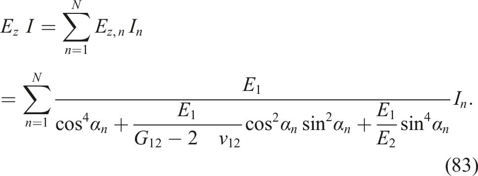
The global elastic modulus of a pipe layer E_z,n is determined by the engineering constants of the single layer E₁, E₂, G₁₂, ν₁₂ and the respective fiber angle α _n according to the approach of Hyer. ⁷² However, this approach does not consider the interaction of the individual layers.

For thick-walled pipes of carbon fiber-reinforced plastic with layer structure [α/− α] the computed flexural stiffnesses following equations (81) and (83) showed a good agreement for fiber angles of α = 0° as well as α > 50°. However, in the 0° < α < 50° section, significantly higher values were found for the calculation according to Jolicoeur and Cardou ⁴⁶ with a maximum deviation of approximately 250 % at fiber angle 15°. ⁷¹ In bending tests on thick-walled tubes (outer diameter 61.1 mm, wall thickness 11.5 mm, length 1016 mm) with layering of [25₄₅/(−25)₄₅] and [25/−25]₉₀ the equivalent bending stiffness ⟨EI⟩ was determined by the maximum axial strain ${\epsilon }_z^{\max }\left(s\right)$ in the pipe center at a deflection s and the adjacent bending moment M _x (s) using

$〈E\hspace{0.17em}I〉=\frac{M_x\left(s\right)}{{\epsilon }_z^{\max }\left(s\right)}\hspace{0.17em}\frac{D_a}{2}.$

(84)

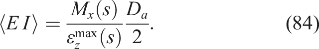
The experimentally obtained equivalent bending stiffnesses of the two pipes according to (84) are denoted by ⟨E I⟩₁ = 29.1 kNm² and ⟨E I⟩₂ = 32.3 kNm². ⁷¹ The values for the approach of strength of materials (83), calculated under the same assumptions, are clearly below the test results with E _z I = 13.5 kNm², while the values calculated using equation (81) according to Jolicoeur and Cardou ⁴⁶ with ⟨E I⟩_1,jol = 33.6 kNm² and ⟨E I⟩_2,jol = 35 kNm² are 8-14 % above the experimental results. ⁷¹ The model according to Jolicoeur and Cardou ⁴⁶ thus provides usable values which are not fully achieved in the experiment due to manufacturing inaccuracies and errors such as porosities and angular deviations.

Furthermore, Shadmehri et al. ⁷³ are concerned with the comparison of the bending stiffness from the classical approach using the moment of inertia according to Hyer ⁷² with an equivalent bending stiffness derived from the non-classical laminated beam theory. This approach is based on the first-order shear deformation theory (FSDT) and considers transverse shear deformations, a coupling between tension and torsion and a coupling between bending and transverse shearing, but no deformations and thus ovalization in the cross-section. By utilizing the elements of the ABD-matrix of the non-classical laminate theory, the mean radius R of the tube and the simplification $\overline{A}=A_{11} A_{33}-A_{13}^2$ , the equivalent bending stiffness can be expressed by

$\begin{array}{l}〈EI〉=R\pi \{R^2(A_{22}-\frac{A_{12}\left(A_{33}\hspace{0.17em}{A}_{12}-A_{13}\hspace{0.17em}{A}_{23}\right)}{\overline{A}}\\ -\frac{A_{23}\left(A_{23}\hspace{0.17em}{A}_{11}-A_{13}\hspace{0.17em}{A}_{12}\right)}{\overline{A}}\\ \cdot \left(A_{66}-\frac{A_{16}\left(A_{33}\hspace{0.17em}{A}_{16}-A_{13}\hspace{0.17em}{A}_{36}\right)}{\overline{A}}-\frac{A_{36}\left(A_{11}\hspace{0.17em}{A}_{36}-A_{13}\hspace{0.17em}{A}_{16}\right)}{\overline{A}}\right)\\ +R^2\left(A_{22}-\frac{A_{12}\left(A_{33}\hspace{0.17em}{A}_{12}-A_{13}\hspace{0.17em}{A}_{23}\right)}{\overline{A}}-\frac{A_{23}\left(A_{23}\hspace{0.17em}{A}_{11}-A_{13}\hspace{0.17em}{A}_{12}\right)}{\overline{A}}\right)\\ \cdot \left(A_{44}\frac{A_{45}^2}{A_{55}}\right)-R^2(A_{26}-\frac{A_{12}\left(A_{33}\hspace{0.17em}{A}_{16}-A_{13}\hspace{0.17em}{A}_{36}\right)}{\overline{A}}\\ {-\frac{A_{23}\left(A_{36}\hspace{0.17em}{A}_{11}-A_{13}\hspace{0.17em}{A}_{16}\right)}{\overline{A}})}^2\\ +2R\left(B_{22}-\frac{A_{12}\left(A_{33}\hspace{0.17em}{B}_{12}-A_{13}\hspace{0.17em}{B}_{23}\right)}{\overline{A}}-\frac{A_{23}\left(A_{11}\hspace{0.17em}{B}_{23}-A_{13}\hspace{0.17em}{B}_{12}\right)}{\overline{A}}\right)\\ \cdot \left(A_{66}-\frac{A_{16}\left(A_{33}\hspace{0.17em}{A}_{16}-A_{13}\hspace{0.17em}{A}_{36}\right)}{\overline{A}}-\frac{A_{36}\left(A_{11}\hspace{0.17em}{A}_{36}-A_{13}\hspace{0.17em}{A}_{16}\right)}{\overline{A}}\right)\\ +2R\left(B_{22}-\frac{A_{12}\left(A_{33}\hspace{0.17em}{B}_{12}-A_{13}\hspace{0.17em}{B}_{23}\right)}{\overline{A}}-\frac{A_{23}\left(A_{11}\hspace{0.17em}{B}_{23}-A_{13}\hspace{0.17em}{B}_{12}\right)}{\overline{A}}\right)\\ \cdot \left(A_{44}\frac{A_{45}^2}{A_{55}}\right)\\ -2R\left(A_{26}-\frac{A_{12}\left(A_{33}\hspace{0.17em}{A}_{16}-A_{13}\hspace{0.17em}{A}_{36}\right)}{\overline{A}}-\frac{A_{23}\left(A_{36}\hspace{0.17em}{A}_{11}-A_{13}\hspace{0.17em}{A}_{16}\right)}{\overline{A}}\right)\\ \cdot \left(B_{26}-\frac{A_{16}\left(A_{33}\hspace{0.17em}{B}_{12}-A_{13}\hspace{0.17em}{B}_{23}\right)}{\overline{A}}-\frac{A_{36}\left(A_{11}\hspace{0.17em}{B}_{23}-A_{13}\hspace{0.17em}{B}_{12}\right)}{\overline{A}}\right)\\ \cdot \left(D_{22}-\frac{B_{12}\left(A_{33}\hspace{0.17em}{B}_{12}-A_{13}\hspace{0.17em}{B}_{23}\right)}{\overline{A}}-\frac{B_{23}\left(A_{11}\hspace{0.17em}{B}_{23}-A_{13}\hspace{0.17em}{B}_{12}\right)}{\overline{A}}\right)\\ \cdot \left(A_{66}-\frac{A_{16}\left(A_{33}\hspace{0.17em}{A}_{16}-A_{13}\hspace{0.17em}{A}_{36}\right)}{\overline{A}}-\frac{A_{36}\left(A_{11}\hspace{0.17em}{A}_{36}-A_{13}\hspace{0.17em}{A}_{16}\right)}{\overline{A}}\right)\\ +\left(D_{22}-\frac{B_{12}\left(A_{33}\hspace{0.17em}{B}_{12}-A_{13}\hspace{0.17em}{B}_{23}\right)}{\overline{A}}-\frac{B_{23}\left(A_{11}\hspace{0.17em}{B}_{23}-A_{13}\hspace{0.17em}{B}_{12}\right)}{\overline{A}}\right)\\ \cdot \left(A_{44}\frac{A_{45}^2}{A_{55}}\right)\\ -{\left(B_{26}-\frac{A_{16}\left(A_{33}\hspace{0.17em}{B}_{12}-A_{13}\hspace{0.17em}{B}_{23}\right)}{\overline{A}}-\frac{A_{36}\left(A_{11}\hspace{0.17em}{B}_{23}-A_{13}\hspace{0.17em}{B}_{12}\right)}{\overline{A}}\right)}^2\}\\ /\{\left(A_{66}-\frac{A_{16}\left(A_{33}\hspace{0.17em}{A}_{16}-A_{13}\hspace{0.17em}{A}_{36}\right)}{\overline{A}}-\frac{A_{36}\left(A_{11}\hspace{0.17em}{A}_{36}-A_{13}\hspace{0.17em}{A}_{16}\right)}{\overline{A}}\right)+\left(A_{44}-\frac{A_{45}^2}{A_{55}}\right)\}.\end{array}$

(85)

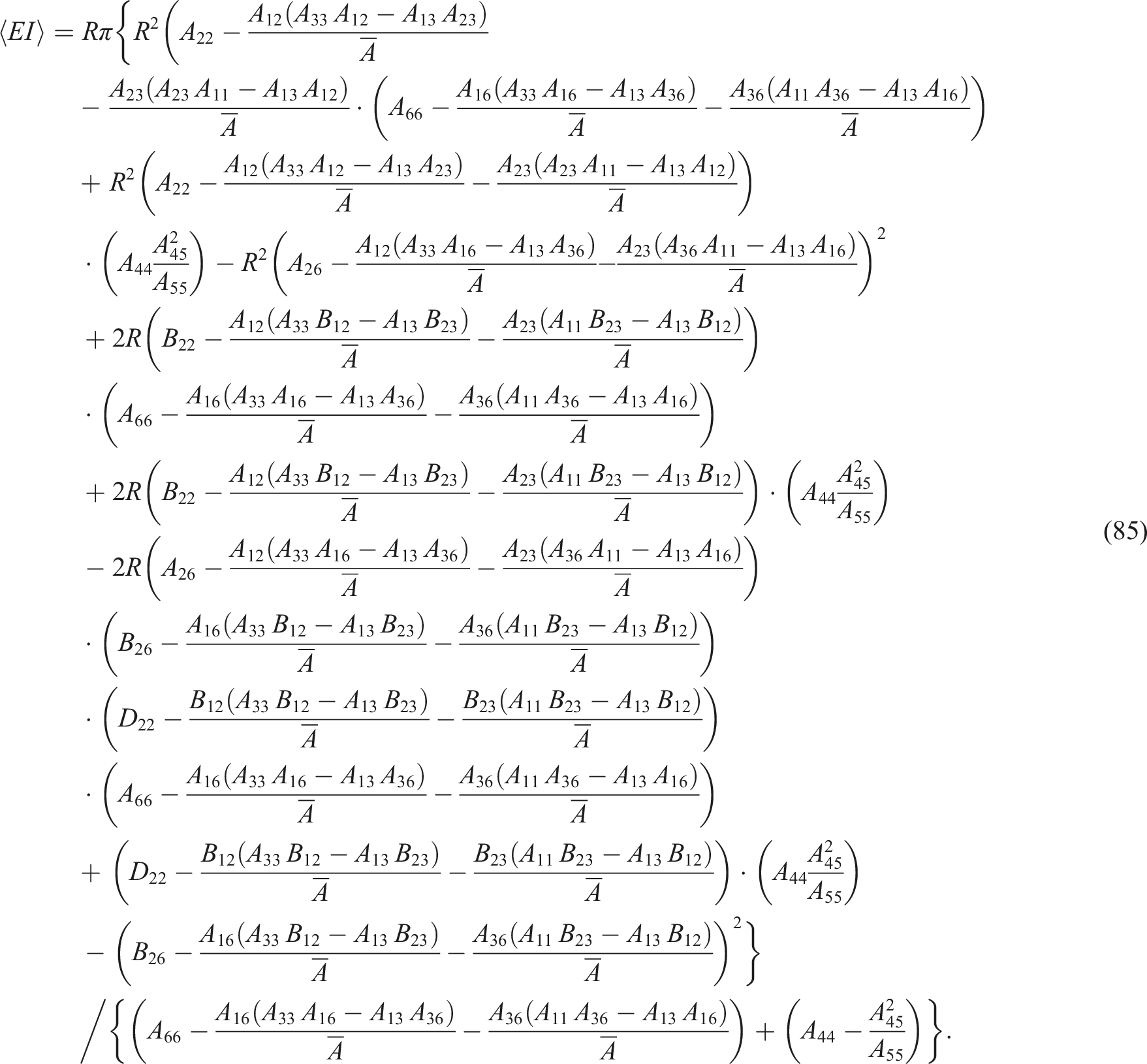
Four different pipe structures [90₂₀/0₂₀], $\left[{\left({90}_{10}/0_{10}\right)}_3/\pm {45}_{25}\right]$ , [90₃₀/±25₄₅/90₅/±30₂₀/90₅/±45₂₀] and [Aluminum 1 mm/90₂₀/±25₂₀/90₅/±30₂₅/90₅/±45₁₀] of carbon fiber-reinforced plastic were examined and compared with three-point and four-point bending tests, respectively. The two theories agree well for pipe type 1 with only approx. 2 % deviation. Shadmehri et al. ⁷³ are linking this to the cross-ply lamination, leaving out the fact that this tube type is the only one which can nearly be assumed thin-walled with a ratio of thickness to mean radius of t/D _m = 0.07. Thinness is given by Zhang et al. ⁴⁸ at a ratio of less than 0.05, which means that all tubes examined by Shadmehri et al. ⁷³ must be considered thick-walled. Although, compared with the cross-ply laminated tubes all other types show significantly higher values of 0.15 to 0.27, which is why an influence can not be ruled out. In bending tests a somewhat lower bending stiffness is achieved than predicted by the non-classical laminated beam theory.

The equivalent bending stiffness from the non-classical laminate theory according to Shadmehri et al., ⁷³ see equation (85), is compared by Derisi et al. ⁷⁴ with a simulation technique in which an equivalent aluminum tube is assigned to a composite pipe and the flexural stiffness is determined by equation (82). First, the composite pipe with inner diameter D _i and wall thickness h is transferred to an equivalent sandwich plate with a core layer of thickness D _i and a respective laminate height h on both sides. This plate has a unit width and the stiffness of the core layer is assumed to be zero. Via classical lamination theory the flexural stiffness is determined for the plate according to

$\begin{array}{ll}{⟨E I⟩}_{\text{plate},\text{CLT}}& =\frac{1}{d_{11}}=\frac{\det \hspace{0.17em}D}{D_{22} D_{66}-D_{26}^2}\\ & =\frac{D_{11} \left(D_{22} D_{66}-D_{26}^2\right)-D_{12} \left(D_{12} D_{66}-D_{26} D_{16}\right)}{D_{22} D_{66}-D_{26}^2}\\ & \frac{+D_{16} \left(D_{12} D_{26}-D_{22} D_{16}\right)}{D_{22} D_{66}-D_{26}^2}.\end{array}$

(86)

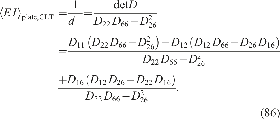
This bending stiffness of the plate does not correspond to the equivalent bending stiffness of the composite pipe, but is proportional to it. ⁷⁴ This bending stiffness is then equated with the bending stiffness of an aluminum sandwich plate of unknown thickness t and unit width. This bending stiffness is

${〈E\hspace{0.17em}I〉}_{\text{plate},\text{alu}}={〈E\hspace{0.17em}I〉}_{\text{plate},\text{CLT}}=1\frac{{\left(D_i+2t\right)}^3-D_i^3}{12}{E}_{\text{alu}}.$

(87)

The sole unknown is the thickness t. Assuming that the core thickness D _i again corresponds to the inner diameter of an aluminum tube with wall thickness t, the equivalent bending rigidity ⟨EI⟩ of the equivalent aluminum tube and therefore the composite tube can now be calculated with equation (82). The procedure is illustrated in Figure 5.

Figure 5.

Schematic representation of the determination of the equivalent flexural rigidity by a comparative method according to Derisi et al. ⁷⁴

For three different laminates and lay-ups both methods were compared with one another and three-point or four-point bending tests, respectively. In the experiment, the force on the compression die and the axial strain on the center of the opposite tube side were recorded. The bending stiffness was then calculated by equation (84). For all types of tubes, which were also used in Shadmehri et al., ⁷³ the closed analytical method according to equation (85) and the comparative technique according to Derisi et al. ⁷⁴ only showed about 2 % difference, while both showed 5-10 % deviation to the experimental results.

Conclusion

All presented tube models have three-dimensional stress, strain and displacement distributions, but show no changes over the tube axis. The approaches for only axisymmetric loads as well as the state-space approaches are furthermore independent of the circumferential coordinate θ. However, even if a dependency is present for the models regarding bending loads, the courses are given by trigonometric initial functions with unknown amplitudes, which is only feasible in tube sections where the St. Vernant principle is applicable. Therefore, the main focus of the models is on the differences in the gradients over the thickness direction r and their formulations of the continuity conditions at the layer transitions, whether their fictious or real. For tubes under bending loads only the stress-based models based on the Lekhnitskii formulation are delievering exact solutions in all three directions without approximations in form of interpolations, series expansions or numeric methods. Beside the differences in the radial distribution and the basic formulation, a distinction of the models in form of the used displacement field is possible. Thus the model of Jolicoeur and Cardou ⁴⁶ allows a warping and rotation of the pipe cross-section that the models of Lekhnitskii ² and Xia et al. ³⁹ are not considering. Further limitations for all models are the assumptions of small deformations and a constant curvature as well as the fact that different load cases are only superposed but not coupled.

In the literature there is no comparison of the different pipe models to be found. Validations of bending models with finite element calculations, if at all, are delivered only for the simplest case of pure bending. An exception to that rule are Sarvestani et al., ⁵⁶ who deal with a tube under cantilever load, although their model is also only applicable in the mid section of the tube far away from load introduction or mounting. Experimental studies are even rarer. Derisi et al., ⁷⁴ Geuchy Ahmad and Hoa ⁷¹ as well as Shadmehri et al. ⁷³ compared different methods to calculate an equivalent bending stiffness and therefore the deflection with three- or four-point bending tests. Only one of these methods is based on an anisotropic, three-dimensional tube model by Jolicoeur and Cardou. ⁴⁶ A more detailed comparison of bending tests on tubes and analytical formulations by Jolicoeur and Cardou ⁴⁶ was carried out by Derisi et al. ⁷⁴ The described models and papers by Sarvestani^45,53–57 included validations with finite element method and experimental studies. Potential for future research work thence lies in the comparison and validation of these models as well as the extension to more complex load cases, such as coupled loads, and the consideration of singularities or inhomogeneities. In addition, it is useful to investigate different symmetry effects of the layer structure and, for example, to consider the influence of the ondulation of the individual layers in the winding process, which turns the positive and negative individual layers into bi-directional individual layers. More on how the winding process of fiber-reinforced plastic tubes affects the bi-directional layers can be read at Kastenmeier. ⁷⁵ Additional studies on the effects of scale reduction can also be carried out. Even though in most cases, calculations using the finite element method are more feasible and accurate.