Sage Journals: Discover world-class research

Abstract

A stochastic cure simulation approach is developed to investigate the variability of the cure process during resin infusion related to thermal effects. Boundary condition uncertainty is quantified experimentally and appropriate stochastic processes are developed to represent the variability in tool/air temperature and surface heat transfer coefficient. The heat transfer coefficient presents a variation across different experiments of 12.3%, whilst the tool/air temperatures present a standard deviation over 1℃. The boundary condition variability is combined with an existing model of cure kinetics uncertainty and the full stochastic problem is addressed by coupling a cure model with Monte Carlo and the Probabilistic Collocation Method and applied to the case of thin carbon epoxy laminates. The overall variability in cure time reaches a coefficient of variation of about 22%, which is dominated by uncertainty in surface heat transfer and tool temperature; with ambient temperature and kinetics contributing variability in the order of 1%.

Keywords

Polymer-matrix composites curing stochastic simulation statistics

Introduction

The manufacturing of composite materials involves many sources of uncertainty associated with material properties and process parameters variability. These uncertainties can considerably influence the properties and the quality of the manufactured part, which in many cases can result in a considerable amount of scrap associated with significant cost and environmental implications. In addition, variability can significantly affect the efficiency of process cycles in terms of time and cost.

The effect of material properties variability has been extensively investigated with a focus on reinforcement geometry. This type of variability is mainly associated with in-plane and out of plane fibre misalignment and can affect all the manufacturing steps. Several experimental studies have indicated that in-plane fibre misalignment can be represented by a normally distributed random variable^1–5 and can present strong spatial autocorrelation over the textile. This can influence the forming process introducing considerable variability in defect generation.⁵ In addition, fibre misalignment alongside nesting effects can introduce significant variability in permeability leading to considerable flow induced defects such as void formation and dry spots.^6–8

The issue of variability during the cure step has received limited attention so far in the literature. The cure process can be potentially affected by material properties variability related to fibre misalignment and resin behaviour uncertainty as well as environmental/boundary condition uncertainty. These effects can influence the risk of the occurrence of cure process defects such as temperature overshoot, under-cure, and shape distortion degrading potentially the overall quality of composite parts. Very limited data and results exist concerning variability during the cure step, whilst the parameters introducing uncertainty into the cure process have not been explicitly characterised and evaluated. The effect of cure kinetics uncertainty and cure temperature uncertainty on cure time has been studied based on hypothesised levels of variability showing that cure temperature variations tend to dominate cure time variability.⁹ Furthermore, consideration of variability in the optimisation of the cure time has shown that optimal cure time increases with increasing variability.¹⁰ A study preceding the work presented here has shown that even in the case of high specification epoxies cure kinetics variability can influence significantly the occurrence of exothermic effects leading to temperature overshoots in thick and ultra-thick components.¹¹ These findings have highlighted the considerable potential practical importance of uncertainty in the cure step and the need for an approach that can be utilised to simulate the overall effect of variability in the outcome of this stage of the process.

This study aims at the investigation of the influence of variability on heat transfer effects occurring during the cure process focusing on cure time. Cure time is of crucial importance since it determines the duration of the manufacturing process which in turn dictates the efficiency and the cost of the process. In addition, variability in cure time can lead to significant amount of scrap since underestimation of the cure time can lead in under-cure resulting in deterioration in the mechanical properties of the part.

A methodology to characterise and model boundary conditions uncertainty related to tool temperature, ambient temperature and surface heat transfer coefficient is developed and the propagation of this variability during the curing process is investigated. This information is combined with existing models of cure kinetics variability¹¹ and the overall stochastic simulation problem is addressed by coupling a finite element based cure simulation model with a Monte Carlo scheme (MC) and an implementation of the Probabilistic Collocation Method (PCM). The methodology is demonstrated in the case of flat thin carbon fibre-epoxy laminates fabricated by resin infusion. During the curing stage of resin infusion processes heat is applied on the surface of the laminate in contact with the mould defined by a cure profile initiating curing reactions. Heat is dissipated due to natural air convection between the vacuum bag and the air resulting to a degree of cure and temperature gradient through the thickness of the laminate. This can result in significant variations in cure time.

Methodology

Cure simulation

A thermal cure simulation model was implemented in the finite element analysis solver MSC.Marc. The model is three dimensional and transient. The modelling approach used in this study was based on 3D iso-parametric 8-node composite brick elements; 175 MSC.Marc element type for thermal analysis. These elements allow modelling of layered materials; different material properties, fibre orientation and thickness can be assigned to different layers within the same element. Each layer contains four integration points and a numerical integration scheme based on Gaussian quadrature is employed. In the case of a flat laminate, the heat transfer problem is solved as a 1D problem with a stack of 3D elements, since the geometry is fully symmetric in the in-plane direction. Therefore, the model of this study comprised six elements as shown in Figure 1; each element comprised of two layers of 0.3 mm thickness, which is the nominal thickness of the fabric used.¹³

Figure 1.

Temperature colour maps; deterministic model.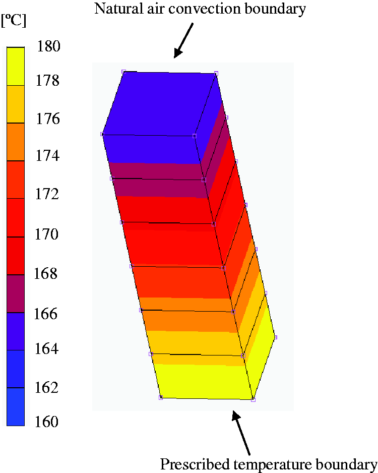

The materials considered were Hexcel RTM6¹² epoxy resin and Hexcel G1157¹³ pseudo unidirectional carbon fibre reinforcement. The material properties of the curing composite depend on both temperature and degree of cure. The material sub-models of cure kinetics, specific heat capacity and thermal conductivity, were implemented in user defined subroutines UCURE, USPCHT and ANKOND,¹⁴ respectively. The cure kinetics model used in this study is a combination of an n^th order model and an autocatalytic model,¹⁵ whilst the specific heat capacity is calculated based on the rule of mixtures. A geometry-based model is applied to compute the thermal conductivity.¹⁶ The specific heat capacity and thermal conductivity of the fibres depend linearly on temperature, whilst the specific heat capacity and thermal conductivity of the resin depend on both temperature and degree of cure. In the cure kinetics model, the cure reaction rate is computed as follows¹⁵

\frac{da}{dt} = k_{1} (1 - a)^{n_{1}} + k_{2} (1 - a)^{n_{2}} a^{m}

(1)

where a is the current degree of cure, k₁, k₂ the reaction rate constants following an Arrhenius law (

k_{1} = A_{1} \exp (- E_{1} / RT), k_{2} = A_{2} \exp (- E_{2} / RT))

, and m, n₁, n₂ the reaction orders. The specific heat capacity is computed using the rule of mixtures as follows¹¹

c_{p} = w_{f} c_{pf} + (1 - w_{f}) c_{pr}

(2)

where w_f is the fibre weight fraction,

c_{pf}

the fibre specific heat capacity and

c_{pr}

the specific heat capacity of the resin. The thermal conductivity in the longitudinal direction is calculated as follows¹⁶

K_{11} = v_{f} K_{lf} + (1 - v_{f}) K_{r}

(3)

where v_f is the fibre volume fraction and

K_{lf}

and K_r are the thermal conductivity of the fibre in the longitudinal direction and of the resin, respectively. In the transverse direction, the thermal conductivity is computed as follows¹⁶

K_{22} = K_{33} = v_{f} K_{r} (\frac{K_{tf}}{K_{r}} - 1) + K_{r} (\frac{1}{2} - \frac{K_{tf}}{2 K_{r}}) + K_{r} (\frac{K_{tf}}{K_{r}} - 1) \sqrt{v_{f}^{2} - v_{f} + \frac{(\frac{K_{tf}}{K_{r}} + 1)^{2}}{(\frac{2 K_{tf}}{K_{r}} - 2)^{2}}}

(4)

where

K_{tf}

is the conductivity of the fibre in the transverse direction.

Details concerning the material sub-models presented in equations (1)–(4) as well the constants required for these models are reported in the literature.¹¹

Experimental setup for the analysis of boundary conditions uncertainty

Investigation of boundary conditions uncertainty was carried out by a series of experiments using an infusion set-up. These experiments aim at characterising the behaviour of stochastic parameters with time as well as across different experimental runs. The information produced forms the basis for the selection and development of appropriate stochastic models of tool temperature, ambient temperature and surface heat transfer coefficient between the vacuum bag and the air.

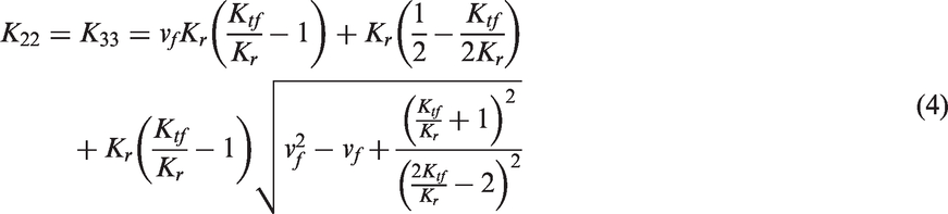
Ten tests were carried out using the experimental set-up illustrated in Figure 2. It comprises an ELKOM 8.4 KW electrical heating platen, a 10 mm thick aluminium tooling plate, a nylon N64PS-x VAC INNOVATION peel ply fabric, a nylon VAClease xR1.2 VAC INNOVATION vacuum bag, two K-type thermocouples and two RdF micro-foil heat flux sensors.¹⁷ A 4.5 mm thick carbon fibre-epoxy flat panel fabricated by infusion was used to produce thermal conditions similar to those during the cure of a part. The matrix system of the panel was Hexcel RTM6, whilst the reinforcement was Hexcel AS7 12 k carbon fibre¹⁸ with an areal density of 268 g/m². The composite panel was placed on the tooling plate, covered with the peel ply and the vacuum bag and sealed before testing. Two heat flux sensors were mounted on the vacuum bag to measure natural air convection variability as well as its spatial dependence. A K-type thermocouple was placed on the tool (T/C1) to quantify tool temperature uncertainty and a second one (T/C2) away from the apparatus to measure ambient temperature variability. The temperature was equilibrated at 160℃ in all tests. The experimental set-up was identical between the different runs, i.e. all the components remained at the same position to ensure maximum possible repeatability in the experimental procedure.

Figure 2.

Schematic representation of cross-section of experimental set-up used for quantification of boundary condition uncertainty.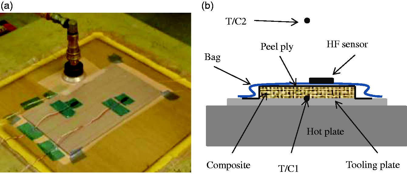

Moreover, additional datasets were acquired to study the effect of signal noise on the experimental results. In particular, two thermocouples and the two heat flux sensors were mounted on the aluminium tooling plate, where one of the thermocouples and one of the heat flux sensors were sealed using a sealing tape used in resin infusion processes. The temperature was equilibrated at 160℃ as well.

The micro-foil heat flux sensor consists of a thin layer as shown in Figure 2 and is a differential thermocouple type sensor using T-type thermocouples.¹⁷ The T-type thermocouples were used to measure the temperature at the vacuum bag. Given that the same heat flux should flow through the sensor and the surface where the sensor is mounted, the sensor is directly measuring the heat loss or gain through the thin layer by measuring the temperature difference between opposite sides of the thin layer. This sensor produces a voltage output which is proportional to heat flux. In particular, the heat-flux $\overset{\cdot}{Q}$ is given by the following relation

\overset{\cdot}{Q} = (HF) / (CM TCF)

(5)

where

HF

is the sensor output,

CM

a calibration multiplier provided by the manufacturer and

TCF

a temperature compensation factor. The calibration multiplier (unique to each sensor) is measured at 21℃ and is not linear with temperature. The sensors used in this study had a calibration multiplier of 0.15 µV per W/m². The temperature compensation factor is a function of temperature and can be found in¹⁷. In the case of the two K-type thermocouples as well as the T-type thermocouples incorporated in the sensors an output in ℃ is produced, whilst in the case of the sensors a voltage output is produced and therefore equation (5) was utilised to calculate the heat flux. Subsequently, the heat transfer coefficient h was computed using the measurements of bag and air temperature T_A

h = \frac{\overset{\cdot}{Q}}{T_{s} - T_{A}}

(6)

where T_s is the temperature at the surface of the bag.

A National Instruments Labview in house code was used for data acquisition and the data were acquired with a frequency of 0.8 Hz.

Stochastic process development

The procedure for selecting and developing the boundary condition stochastic models uncertainty is illustrated in Figure 3. The first step is to estimate the autocorrelation structure of the raw data for each variable in order to investigate the dependence of variability on time. In the case of a stationary process, no trend is present in the data and the autocorrelation decays close to the zero value within several time increments. If the autocorrelation is close to zero on average, the time series is considered a random sequence of observations that are independent and therefore can be modelled as a random variable. If the autocorrelation does not decay towards a negligible plateau in the long term, i.e. the population shows strong autocorrelation with time (the population presents a trend over time) then the process is considered non-stationary and de-trending needs to be applied in order to generate a stationary stochastic process (Figure 3). After removing the trends, the residual variability is modelled using a stationary stochastic process. This procedure is repeated for every experimental curve of the three parameters to model variability across the different experimental runs.

Figure 3.

Schematic representation of methodology for modelling of boundary conditions uncertainty.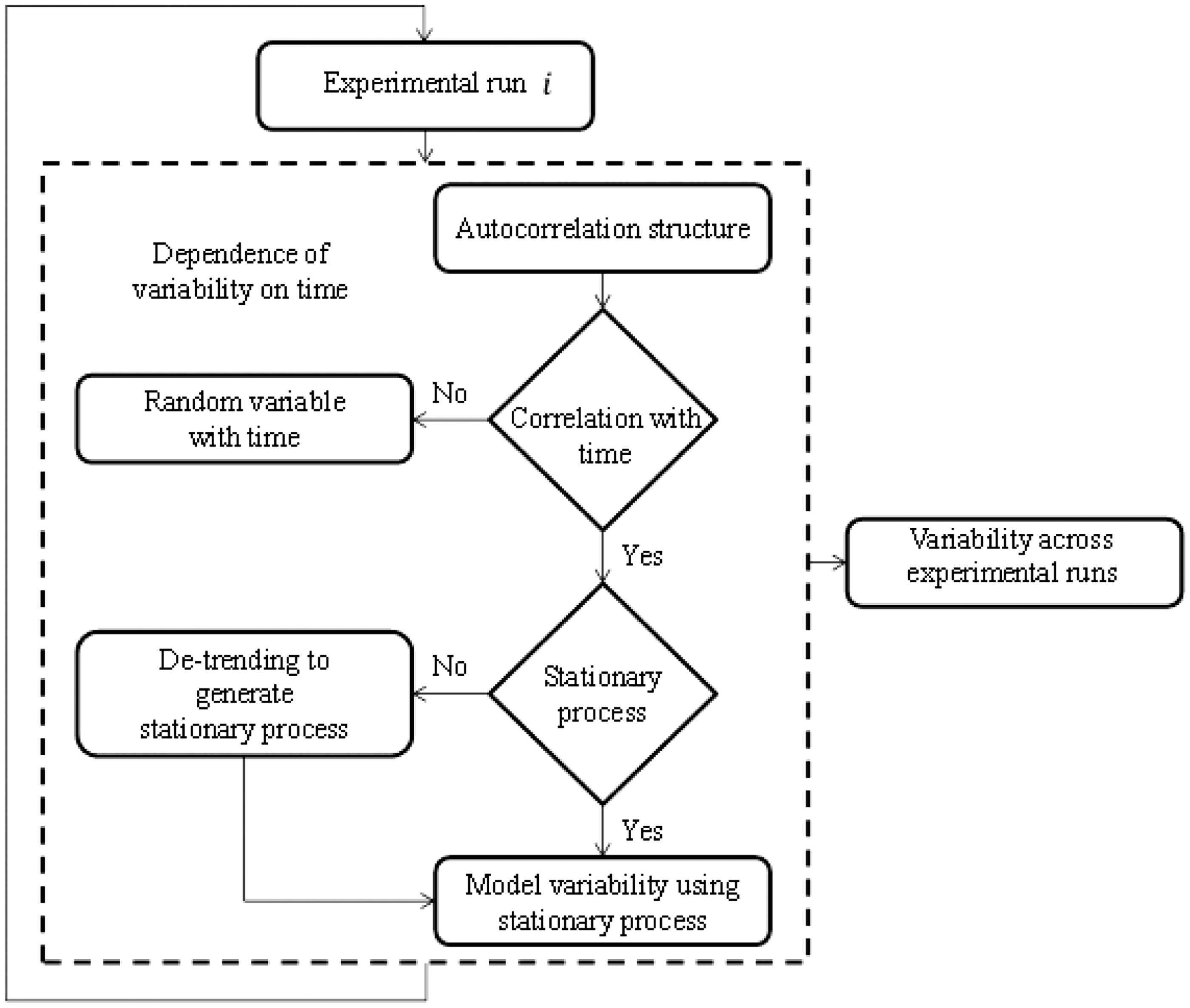

Stochastic simulation approach

Investigation of variability in thermal effects during the curing process requires the development and implementation of a stochastic simulation methodology. Here the focus is to estimate the influence of variability on cure time. Cure time is considered as the time at which the minimum degree of cure of the laminate is greater than 0.9.

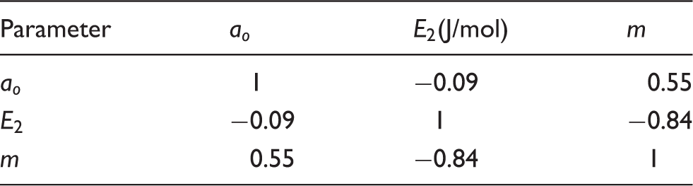
The simulation is carried out using the Monte Carlo (MC) method. This is based on the generation of realisations of the random variables involved in the simulation which are output to the cure model through a programmatic interface which interacts with the text files implementing the finite element solution. The interface calls the execution of the cure model solution and upon completion reads the corresponding output which is translated to cure time and stored. The implementation of the Monte Carlo method includes a step of Cholesky decomposition¹⁹ which is activated when some of the variables are correlated. In the simulation executed in this study this was only necessary for the stochastic parameters of the cure kinetics models as detailed in the literature.¹¹

The use of crude Monte Carlo is computationally intensive and could limit applicability of stochastic simulation in cases the cure model involves a large number of degrees of freedom or iterative execution is necessary, e.g. when the stochastic simulation is used alongside numerical optimisation. The Probabilistic Collocation Method (PCM) was tested as an efficient modification. The main concept of the collocation method is to construct a response surface for each output parameter as a function of the uncertain parameters in the form of orthogonal polynomials and then carry out uncertainty analysis using this surrogate model. The unknown polynomial coefficients are computed using the probabilistic collocation approach at a set of collocation points.²⁰ The collocation points are the roots of the next higher order orthogonal polynomial than the order of the response surface and are chosen so that the residuals between each response surface and the actual model output are zero.²⁰

In the implementation of the collocation method in this study, a third order response surface was constructed to represent cure time as a function of the stochastic parameters. A modified regression-based collocation approach was implemented to improve accuracy. In modified regression collocation, the number of collocation points used is larger than the number of the unknown polynomial coefficients, implying that the effect of each collocation point is reduced.²⁰ In the particular application of PCM addressed here, which involved three stochastic parameters, the number of the unknown coefficients for a three dimensional third order polynomial is 20²⁰ and 39 collocation points were used. As a result, 19 additional deterministic model runs were required, however; the additional computational cost for the given case was negligible since the running time of one deterministic model run was only a few seconds.

Therefore, the final Monte Carlo simulation using the surrogate model based on the PCM representation requires only 39 evaluations of the cure model.

Enquiries for access to the data referred to in this article should be directed to researchdata@cranfield.ac.uk.

Boundary conditions uncertainty

Experimental results

Figures 4 –6 summarise the experimental results of tool temperature, ambient temperature and surface heat transfer coefficient evolution for the ten tests. Note that in all three figures, the x-axis starts at 100 min due to the fact that this was the amount of time the controller required to reach a plateau around 160℃ for the different experimental runs. A variable level across the different experimental runs is observed for all three parameters. This implies that in addition to time variations there is a dependence of the underlying level of each parameter across the different runs. The results obtained by the sensor noise investigation showed that the short term variability presented in Figures 4 –6 can be attributed to the motion of air streams at a local level rather than signal noise effects.

Figure 4.

Tool temperature as a function of time.

Figure 5.

Ambient temperature as a function of time.

Figure 6.

Surface heat transfer coefficient as a function of time.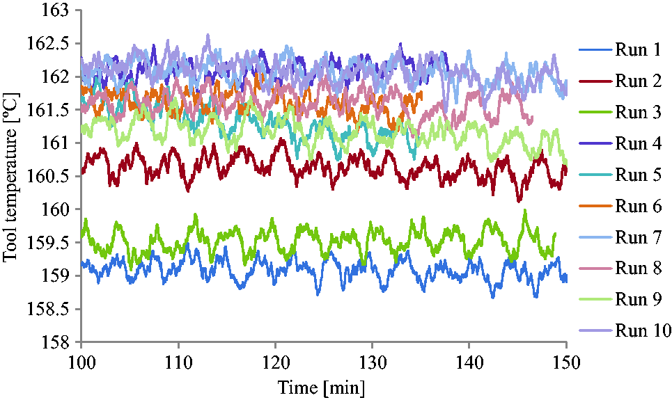

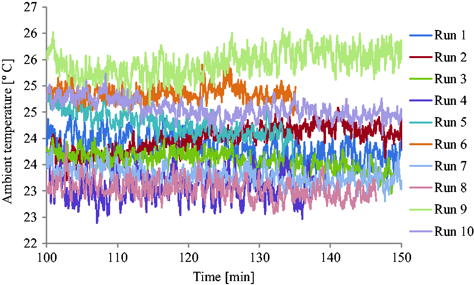
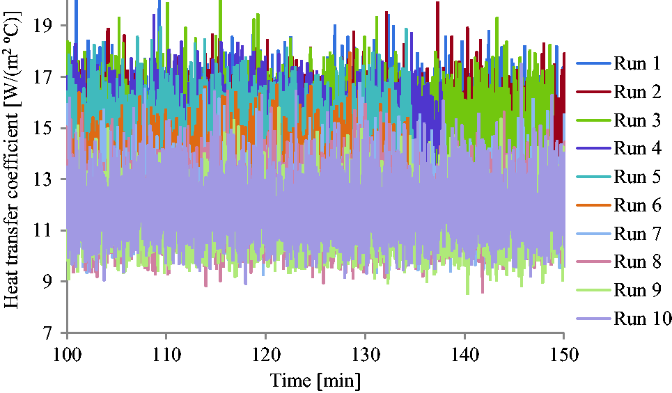
In terms of time dependence, the tool temperature presents a periodic trend and short term variability as shown in Figure 4. The periodic trend is more pronounced and is governed by the temperature controller, whilst short term variability is due to random variations. The periodic features presented here correspond to the tooling set up of this study. It is expected that in the case of a larger components and more complex geometries deviations from the nominal set point can be higher resulting in a periodic trend of higher amplitude. The ambient temperature measurements exhibit a non-periodic long term trend and short term variability (Figure 5). This behaviour is attributed to several factors including the local temperature conditions, humidity, the use of heating or cooling systems and the quality of the insulation of the laboratory. The differences between the results obtained by the two heat flux sensors placed at different location on the vacuum bags were negligible implying that for the given case there is no spatial dependence of the surface heat transfer variability. The surface heat transfer coefficient shows short term variability and a variable level. This type of variability can be attributed to the fact that natural air convection is driven by buoyancy forces caused by density differences due to temperature variations in air. As temperature increases, the density of the fluid in the boundary layer decreases which causes the fluid to rise and be replaced by cooler fluid that also will heat and rise. Consequently, natural air convection is strongly influenced by the motion of air streams at a local level. In addition, variability in radiation (windows) caused by variations in day weather as well as the presence of different people in the lab can introduce variability in surface heat transfer coefficient. All these effects reflect real life applications.

No correlation is expected between the three parameters since tool temperature is solely dependent on the controller, ambient temperature is dictated by environmental conditions such as weather, radiation from windows, humidity, whilst natural air convection is mainly influenced by the motion of air streams at a local level. Indeed, the experimental results showed that there is no correlation between the three variables presenting a correlation coefficient below 0.03 implying that variability is generated independently between the three variables.

Stochastic processes

Figure 7 illustrates the autocorrelation structure for one experiment (Run 1) for the three variables. Each variable has identical autocorrelation structure across different runs. Both tool temperature and ambient temperature present long term strong autocorrelation (Figure 7(a) and (b)) implying non-stationary processes. Autocorrelation measures the extent to which variation of a variable behaves similarly for specific time lags. A periodic and a constant autocorrelation structure are observed in the case of tool temperature and ambient temperature, reflecting the periodic trend (Figure 4) and linear trend (Figure 5) in the experimental data, respectively. Note that the negative autocorrelation presented in Figure 7 is due to the periodic nature of tool temperature variability as shown in Figure 4.

Figure 7.

Autocorrelation as a function of time lag- Run 1: (a) tool temperature; (b) ambient temperature; (c) surface heat transfer coefficient.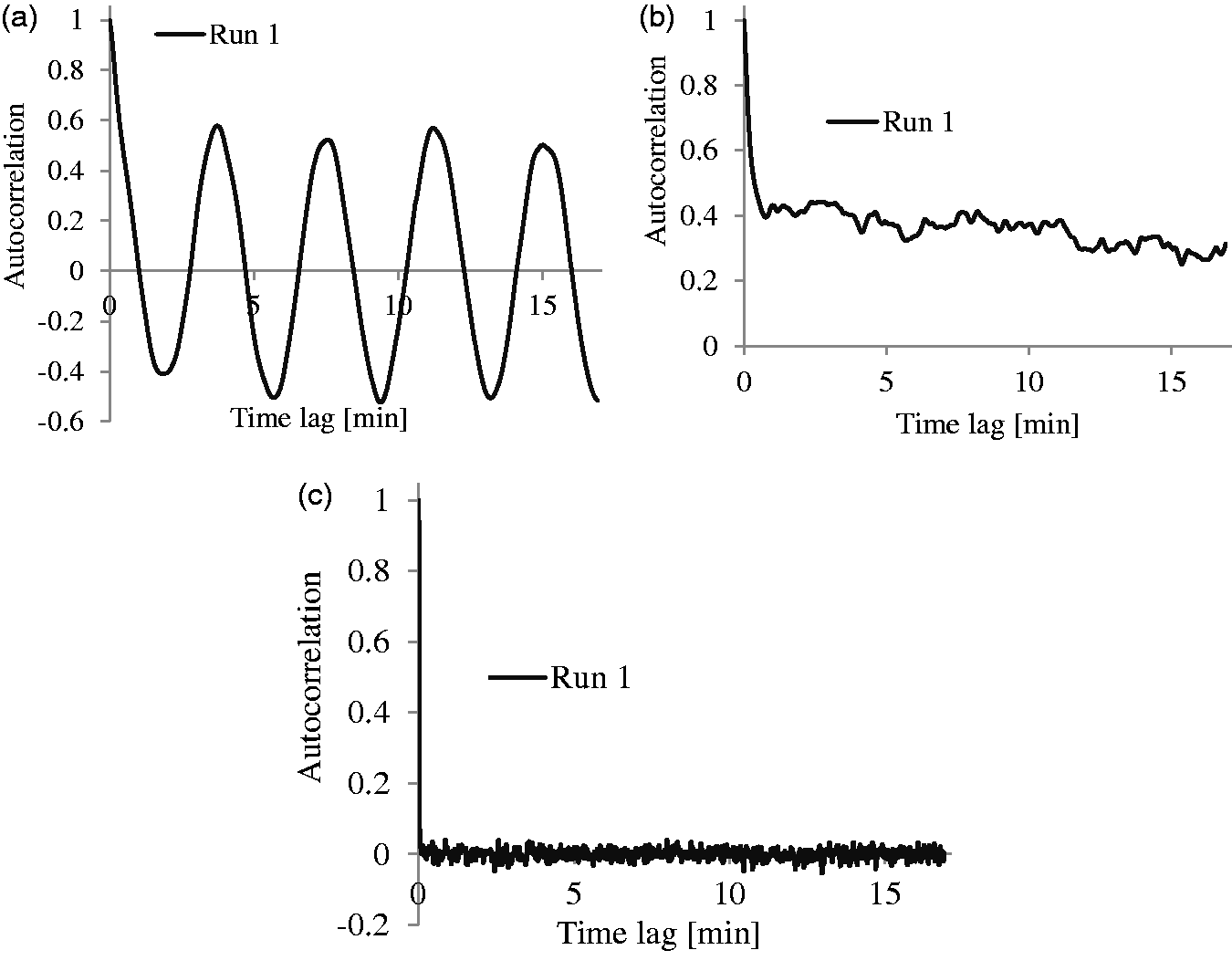

Consequently, de-trending needs to be applied to generate stationary stochastic processes for these two variables. The stationary stochastic process adopted to represent the ambient and tool temperature residuals after de-trending was the Ornstein-Uhlenbeck process (OU), which is a mean reverting second order stationary Gaussian random process. The stochastic differential equation of this process S is the following²¹

ds = λ (μ - S) dt + σ d W_{t}

(7)

Here W_t is a Brownian motion which follows a normal distribution with mean 0 and standard deviation 1 so that

W_{t} ~ N (0, 1)

, whilst

{dW}_{t}

follows a normal distribution with mean 0 and standard deviation

\sqrt{dt}

so that

{dW}_{t} ~ N (0, \sqrt{dt})

, λ controls the speed of reversion to the long term mean of the process, μ is the long term mean of the stochastic process and σ the process volatility. The stochastic differential equation expressed by equation (7) can be integrated analytically,²¹ which implies benefits with respect to integration and the possibility for the use of a relatively large time steps in simulation.

In the case of surface heat transfer coefficient, the autocorrelation structure shows a fast decay reaching a value close to zero after the first lag of time, implying that heat transfer coefficient shows no serial correlation over time (Figure 7(c)). Therefore, the surface heat transfer coefficient can be treated as a random series of observations over time and modelled as follows

h = A_{h} + B_{h} y

(8)

where A_h expresses the level and is the mean value and B_h the volatility of the process for each experimental run, whilst y is a standard normal variable.

Figure 8 illustrates the results obtained in the different steps of the analysis of tool temperature variability. Fast Fourier transform (FFT) implemented in Matlab was used to estimate the frequency of the periodic component of the process shown in Figure 3. A cosinusoidal fit (Figure 8(a)) was performed using the generalised reduced gradient non-linear optimisation method implemented in Microsoft Excel²² to obtain an estimate of the amplitude of the periodic component. The residuals from the cosinusoidal fit present strong autocorrelation; therefore linear regression was applied to the residuals to remove the remaining trend as shown in Figure 8(b). The residuals from the linear fit were modelled using equation (7). Figure 8(d) illustrates the autocorrelation of simulated residuals of tool temperature generated using a time increment of 1.25 s. It can be observed that the OU process reproduces the decay of the autocorrelation structure successfully. There are some discrepancies in the region of the plateau; however, this introduces a negligible error since the autocorrelation is close to zero at this region.

Figure 8.

Procedure of modelling of tool temperature uncertainty: (a) cosinusoidal fit; (b) linear fit; (c) modelling of stationary process; (d) autocorrelation of simulated residuals over time.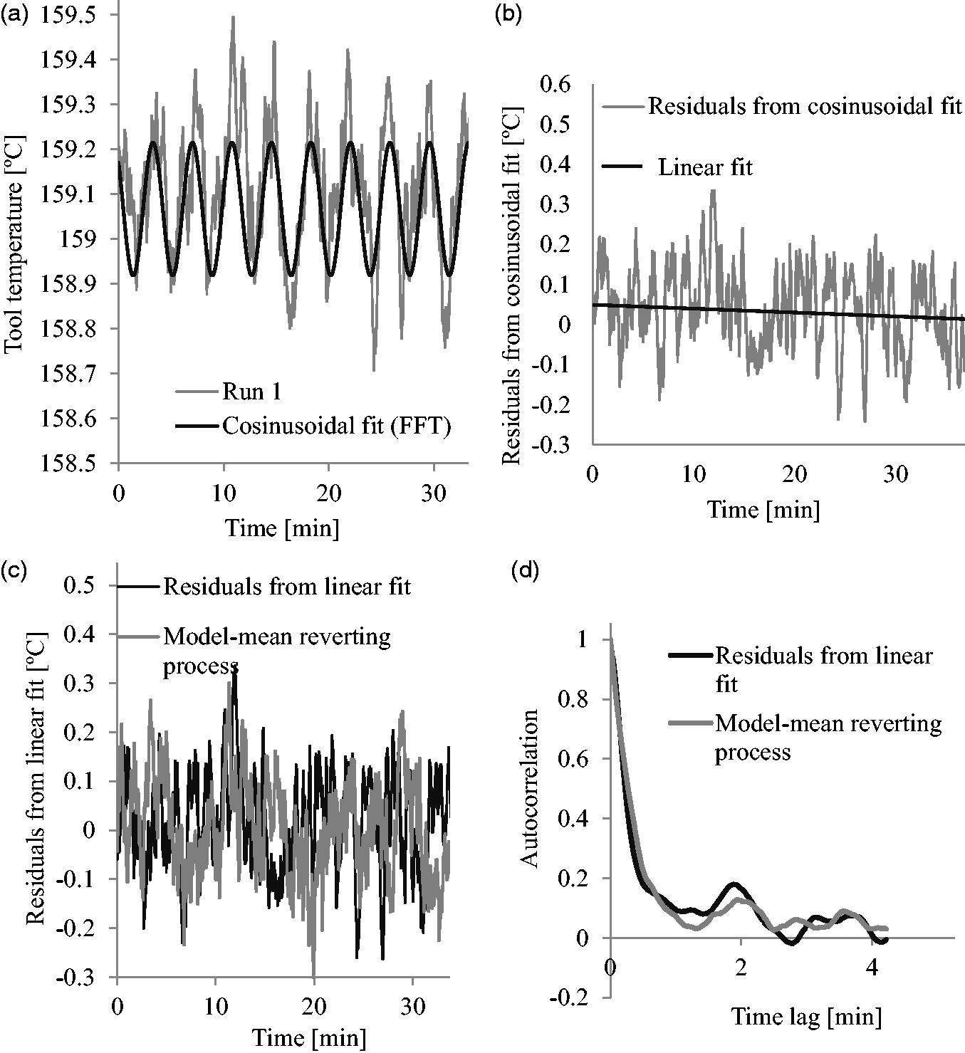

This procedure was iterated for every experimental run and yielded the following stochastic equation

T_{T} = A_{T} + B_{T} t + C_{T} \cos (ω_{T} t) + S_{T}

(9)

The first two terms express the linear fit and represent the level and slope of each experimental curve, whilst C_T and

ω_{T}

are the amplitude and the frequency of the cosinusoidal fit, respectively. In addition, S_T expresses the mean reverting stationary stochastic process (OU) and can be calculated by integrating equation (7).

Figure 9 shows the analysis steps in the case of ambient temperature variability. As shown in Figure 9(a), a linear fit was carried out to remove the long term trend in ambient temperature over time. The residuals resulting from the linear fit presented strong autoregression (Figure 9(b)) and were modelled using equation (7). Figure 9(c) illustrates the autocorrelation of simulated residuals of ambient temperature generated using a time increment of 1.25 s. Similarly to tool temperature, the OU process is capable of capturing the decay of the autocorrelation structure successfully.

Figure 9.

Procedure of modelling of ambient temperature uncertainty: (a) linear fit; (b) modelling of stationary process; (c) autocorrelation of simulated residuals over time.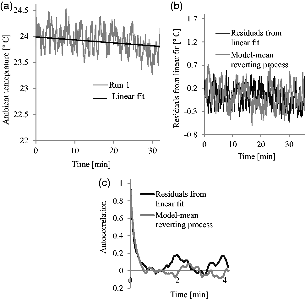

Ambient temperature variability was modelled using the following stochastic relation

T_{A} = A_{A} + B_{A} t + S_{A}

(10)

where A_A and B_A are the constants of the linear fit and represent the level and slope of each experimental curve, and S_A is a mean reverting stochastic process expressed by equation (7).

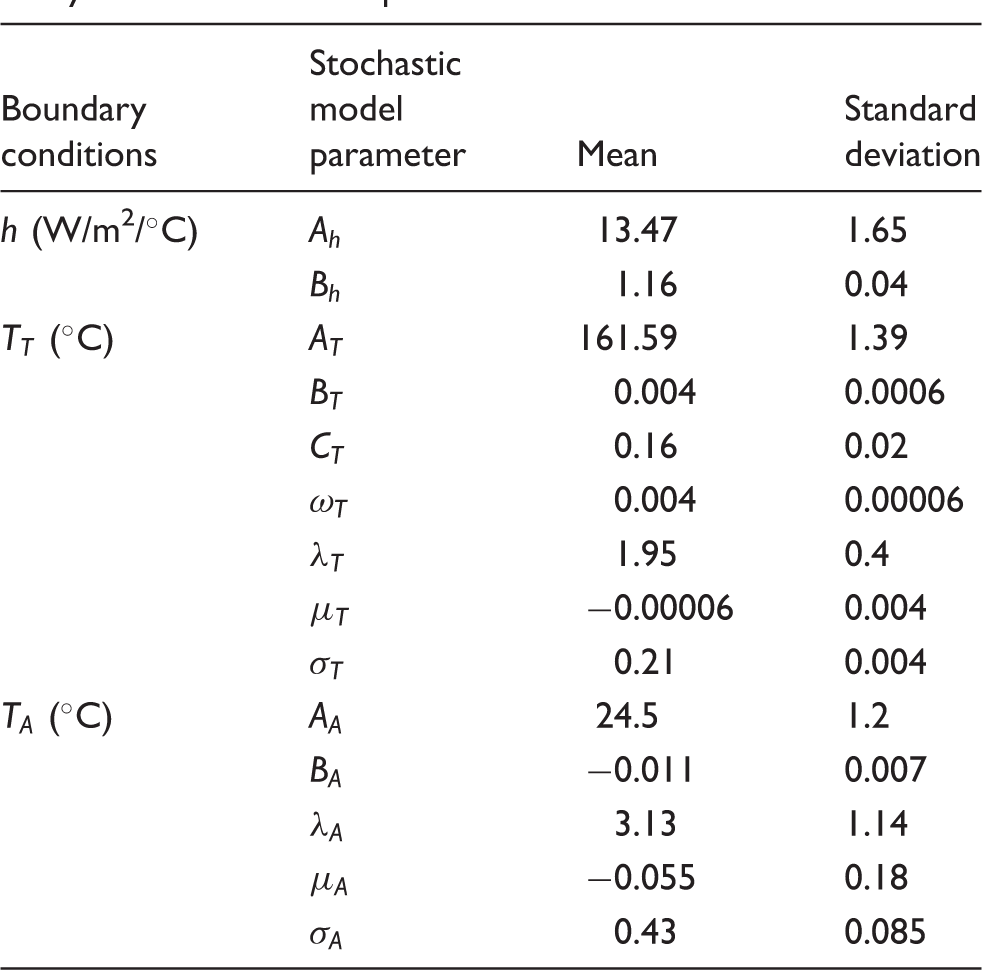
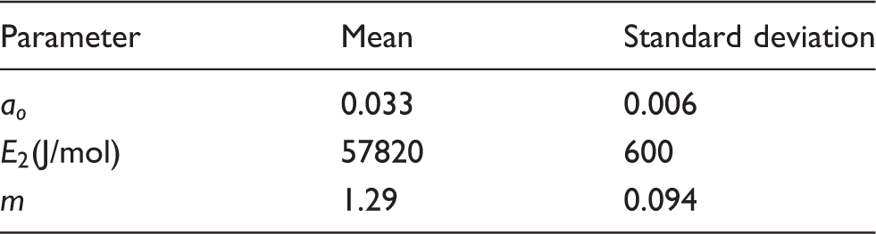
All terms in equations (8) to (10) were estimated for each experimental curve for the three parameters and were considered normal random variables across different runs and constant with time.

Table 1 summarises their statistical properties. Examination of Table 1 suggests that all three variables (tool/ambient temperature, heat transfer coefficient) present a significant variation in level (A_h, A_T, A_A) across the different runs with the surface heat transfer coefficient showing the highest variability. The mean value of

λ_{A}

is considerably higher than that of

λ_{T}

, implying that ambient temperature shows stronger autoregression than tool temperature.

Table 1.

Statistical properties of boundary conditions uncertainty across different experimental runs.

Boundary conditions	Stochastic model parameter	Mean	Standard deviation
h (W/m²/℃)	A_h	13.47	1.65
h (W/m²/℃)	B_h	1.16	0.04
T_T (℃)	A_T	161.59	1.39
	B_T	0.004	0.0006
	C_T	0.16	0.02
	$ω_{T}$	0.004	0.00006
	$λ_{T}$	1.95	0.4
	$μ_{T}$	−0.00006	0.004
	$σ_{T}$	0.21	0.004
T_A (℃)	A_A	24.5	1.2
	B_A	−0.011	0.007
	$λ_{A}$	3.13	1.14
	$μ_{A}$	−0.055	0.18
	$σ_{A}$	0.43	0.085

Stochastic cure simulation

The cure of a 3.6 mm thick carbon fibre- epoxy laminate fabricated by infusion was modelled using the stochastic simulation approach developed in this study. The lay-up sequence of the laminate was [0°/90°/90°/0°]₃. The model comprised the laminate only (Figure 1) since the purpose of this study was to investigate the influence of boundary conditions variability on the process of cure. Therefore, prescribed temperature boundary condition defined by the cure profile was applied to the nodes in contact with the mould, whereas a natural air convection boundary condition was applied on the surface in contact with the vacuum bag as shown in Figure 1. Variability in tool temperature was measured at the surface of the aluminium tool which was in direct contact with the laminate as detailed in Experimental setup for the analysis of boundary conditions uncertainty section . Therefore, the contact resistance between the aluminium tool and the hot plate was not modelled since it does not affect the process. The heat transfer problem of this study is solved as a 1D problem with a stack of 3D elements, therefore, adiabatic boundary conditions were applied at the lateral walls of the laminate assuming no heat loss due to the high width to thickness ratio. The standard cure profile for the epoxy system of this study (Hexcel RTM6) was used comprising two dwells at two different temperatures linked by two standard ramps of 1℃/min. The temperature of the first dwell T₁ as well as the post cure temperature T₂ are considered stochastic following equation (9). In the case of T₂ the mean value of A_T is set at 180℃. The initial temperature was set at 120℃ which is the initial temperature of the nominal cure profile for RTM6.

A time increment of 1 min was used in the cure simulation and the three parameters were set at the mean values of A_h, A_T and A_A, respectively. Figure 1 presents the final temperature distribution through the thickness of the laminate for the deterministic simulation. A temperature gradient of about 4.4℃/mm is observed due to heat dissipation at the top of the laminate caused by natural air convection. Figure 10 presents deterministic cure simulation results at three different points across the thickness of the laminate. The three points are located at the lower boundary (prescribed temperature boundary condition), middle and top (natural air convection boundary condition) of the laminate. An out of plane degree of cure gradient is present due to heat dissipation caused by natural air convection at the top of the laminate. This leads to different degree of cure and cure reaction rate evolution through the thickness of the laminate, as shown in Figure 10. The onset of the reaction is shifted towards higher times from the lower side to the top of the laminate. This is explained by the presence of a temperature gradient through the thickness of the laminate (Figure 1); the temperature at the top of the laminate is lower than the control temperature throughout the cycle resulting in a lag in reaction progress. Similarly, the degree of cure at the end of the cycle is maximised on the lower face with a value of 0.95, in contrast to a final value of 0.91 at the upper face of the curing component (Figure 10).

Figure 10.

Evolution of laminate degree of cure and temperature through the thickness of the laminate. Deterministic model results.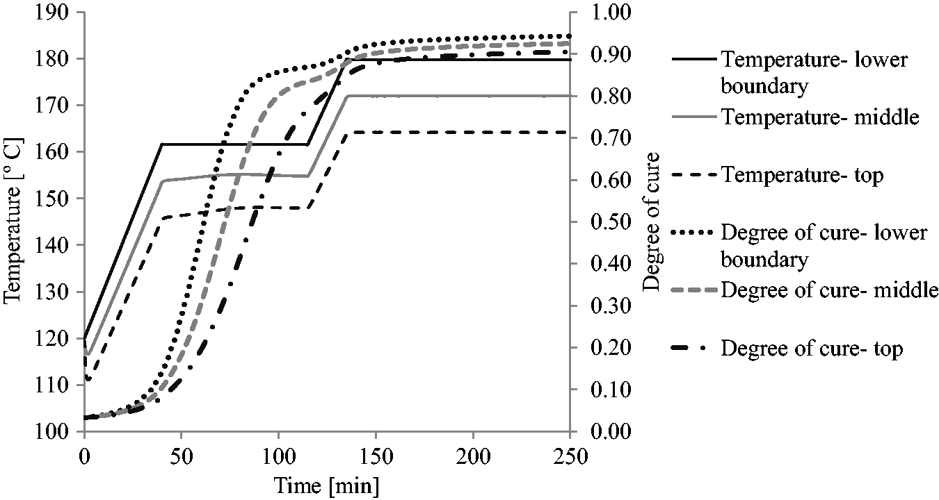

Short term variability

The effect of variability over time for the three parameters was investigated to study the influence of short term variability on the process outcome. This was carried using equations (8) to (10) assuming constant values for A_h, A_T and A_A equal to the corresponding means. Three cases were considered; surface heat transfer coefficient uncertainty over time only, tool temperature variability over time only and ambient temperature variability over time only. A time increment of 1.25 s was used in all three cases in order to reproduce the dependence of variability on time for these parameters accurately, increasing significantly the computational cost.

Table 2 summarises the stochastic simulation results for the three cases. Figures 11 –13 present the evolution of temperature and degree of cure for the three cases, respectively.

Table 2.

Stochastic simulation results; effect of variability over time on cure time.

Case	Mean (min)	Standard deviation (min)
Deterministic	207.69	-
h	207.62	0.19
T_T	207.68	0.021
T_A	207.69	0.016

Figure 11.

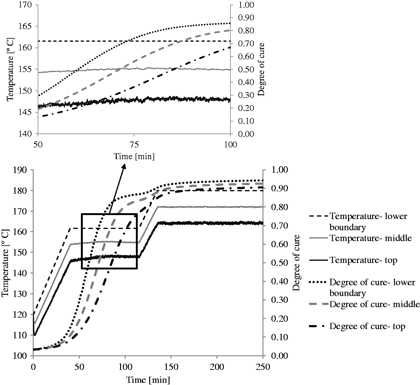
Surface heat transfer coefficient variability over time; evolution of laminate degree of cure and temperature through the thickness of the laminate. Inset: detail during the first dwell.

Figure 12.

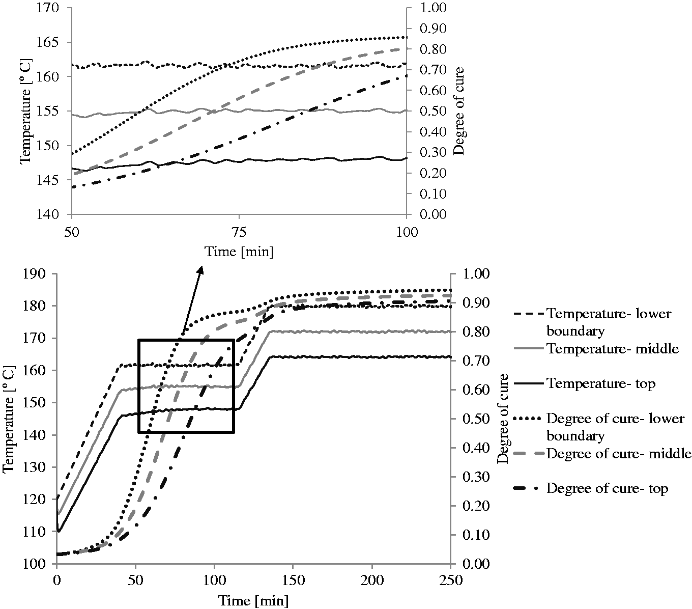
Tool temperature variability over time; evolution of laminate degree of cure and temperature through the thickness of the laminate. Inset: detail during the first dwell.

Figure 13.

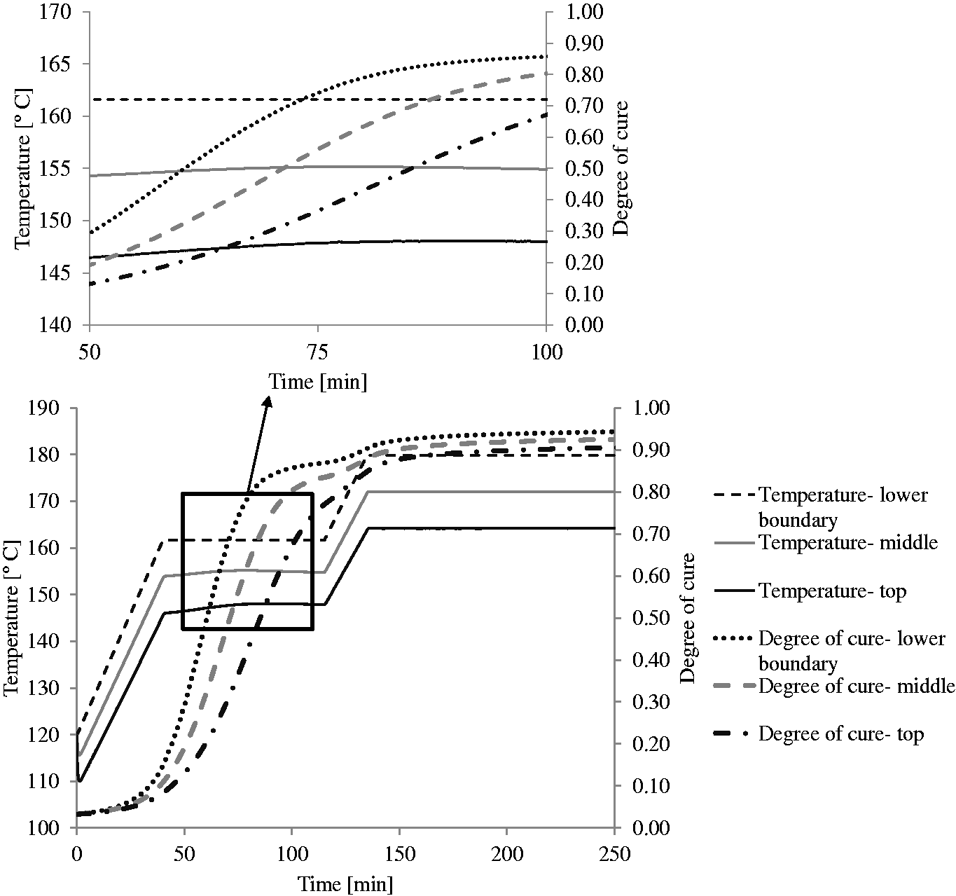
Ambient temperature variability over time; evolution of laminate degree of cure and temperature through the thickness of the laminate. Inset: detail during the first dwell.

In the case of surface heat transfer coefficient variability over time (Figure 11), the temperature at the natural air convection boundary condition presents variations governed by variations in surface heat transfer coefficient with time. The temperature at the middle of the laminate presents a considerably weaker variation with lower volatility, whilst the evolution of degree of cure through the thickness of the laminate is not affected implying that time variations in surface heat transfer coefficient uncertainty introduce negligible variability on the cure process outcome. In particular, the absolute differences in the degree of cure between this case and the deterministic model vary from 9 × 10⁻⁸ to 5 × 10⁻⁵.

In the case of tool temperature variability over time, the temperature at the temperature boundary condition shows a periodic trend reflecting the periodic trend of tool temperature (Figure 12). Similar behaviour is observed through the thickness of the laminate, implying that tool temperature variations propagate evenly through the thickness of the laminate; however, the evolution of degree of cure through the thickness of the laminate is not influenced with the absolute differences in the degree of cure between this case and the deterministic model varying from 8 × 10⁻⁸ to 7 × 10⁻⁵.

Time variations of ambient temperature uncertainty introduce negligible variability in the temperature field and consequently in the degree of cure of the laminate (Figure 13) due to the fact that ambient temperature plays a less important role in heat dissipation caused by natural air convection. The absolute differences between this case and the deterministic model vary from 9 × 10⁻⁸ to 5.5 × 10⁻⁵.

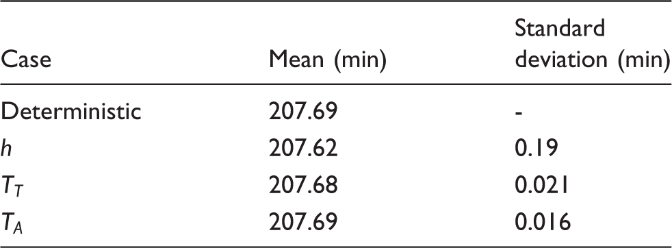
These results show that time variability has a negligible influence on the outcome of the process. This is due to the fact that for the given spread of values, the autoregressive nature of the stochastic parameters compensates their instantaneous variations over time introducing negligible variability to the cure process outcome. The stochastic simulation results indicate that variability over time introduces negligible variations in cure time, with a coefficient of variation of 0.9%, 0.01% and 0.007% for the surface heat transfer coefficient, tool temperature and ambient temperature, respectively. In addition, the mean value of cure time converges to the corresponding nominal value resulting from the deterministic simulation in all three case studies, implying that the response of the model is not biased by short term variability. Therefore, stochastic simulation using the three levels as the only stochastic parameters and a time increment of 1 min in the simulations is sufficient to capture variability propagation accurately.

Effect of level variability across different runs

Following from the results of the previous section, the overall simulation can be carried out considering the variability of the level of surface heat transfer coefficient and tool and air temperature. Thus, equations (8) to (10) can be truncated to

h = A_{h}

(11)

T_{T} = A_{T}

(12)

T_{A} = A_{A}

(13)

In addition to boundary conditions variability, the effect of cure kinetics uncertainty can be considered using the uncertainty model detailed in the literature.¹¹

Variability in cure kinetics (equation (1)) is attributed in variations in the initial degree of cure a_o, activation energy E₂ and reaction order m.¹¹ Tables 3 and 4 summarise the statistical properties and the correlation matrix of the three stochastic variables, respectively. The correlation matrix expresses the cross-correlations between the three stochastic variables so that its

i, j

entry is the correlation coefficient between the corresponding cure kinetics parameters.

Table 3.

Statistical properties of stochastic cure kinetics parameters.¹¹

Parameter	Mean	Standard deviation
a_o	0.033	0.006
E₂(J/mol)	57820	600
m	1.29	0.094

Table 4.

Correlation matrix of stochastic cure kinetics parameters.¹¹

Parameter	a_o	E₂(J/mol)	m
a_o	1	−0.09	0.55
E ₂	−0.09	1	−0.84
m	0.55	−0.84	1

Five different cases were investigated using Monte Carlo taking into account: (i) cure kinetics and boundary conditions uncertainty, (ii) cure kinetics uncertainty only, (iii) ambient temperature variability, (iv) tool temperature variability and (v) surface heat transfer coefficient variability. The stochastic simulation results for the five cases are summarised in Table 5. Considering a convergence criterion of 5% of coefficient of variation in the standard deviation of cure time, satisfactory convergence is obtained in the Monte Carlo simulation after 1000 iterations for the first and last cases, whilst 500 iterations are required for the rest. The relative difference between the mean of cure time when considering variability in h and T_t and the mean of cure time when considering all sources of variability is below 1% (Table 5), implying that there is no significant bias when h and T_t are considered stochastic.

Table 5.

Stochastic cure simulation results; effect of level variability on cure time.

Case	Mean (min)	Standard deviation (min)
Kinetics, h, T_T, T_A	217.97 (MC)	47.41 (MC)
h	215 (MC)	37.4 (MC)
T_T	212.6 (MC)	25.7 (MC)
T_A	207.7 (MC)	2.31 (MC)
Kinetics	208.3 (MC)	2.63 (MC)
h, T_T	219.7 (MC), 218.6 (PCM)	49.5 (MC), 47.8 (PCM)

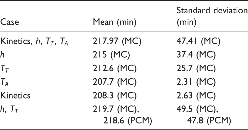
Figure 14 illustrates the probability distribution of cure time for the five cases. The results suggest that cure time presents a coefficient of variation of 21.8%, 1.2%, 1.1%, 12% and 17.4% (standard deviation of 47.4, 2.6, 2.3, 25.7 and 37.4 min) for the five cases. Examination of the probability distribution for the different cases shown in Figure 14 indicates that cure time can be considered a normally distributed random variable. These findings show that the surface heat transfer coefficient and tool temperature dominates cure time variability. Cure kinetics (Figure 14(b)) and ambient temperature (Figure 14(c)) uncertainty affect cure time variability; however, their influence is weak compared to variations in surface heat transfer coefficient and tool temperature as shown in Figure 14(a), (d) and (e), respectively. Furthermore, the mean value of cure time converges to the corresponding nominal value resulting from the deterministic simulation in the second and third cases, whilst is slightly higher in for the rest. This implies that there is a non-linear relation between cure time and surface heat transfer and tool temperature.

Figure 14.

Cumulative probability distribution of cure time: (a) boundary conditions and cure kinetics uncertainty; (b) cure kinetics uncertainty only; (c) ambient temperature variability only; (d) tool temperature variability only; (e) heat transfer coefficient uncertainty only.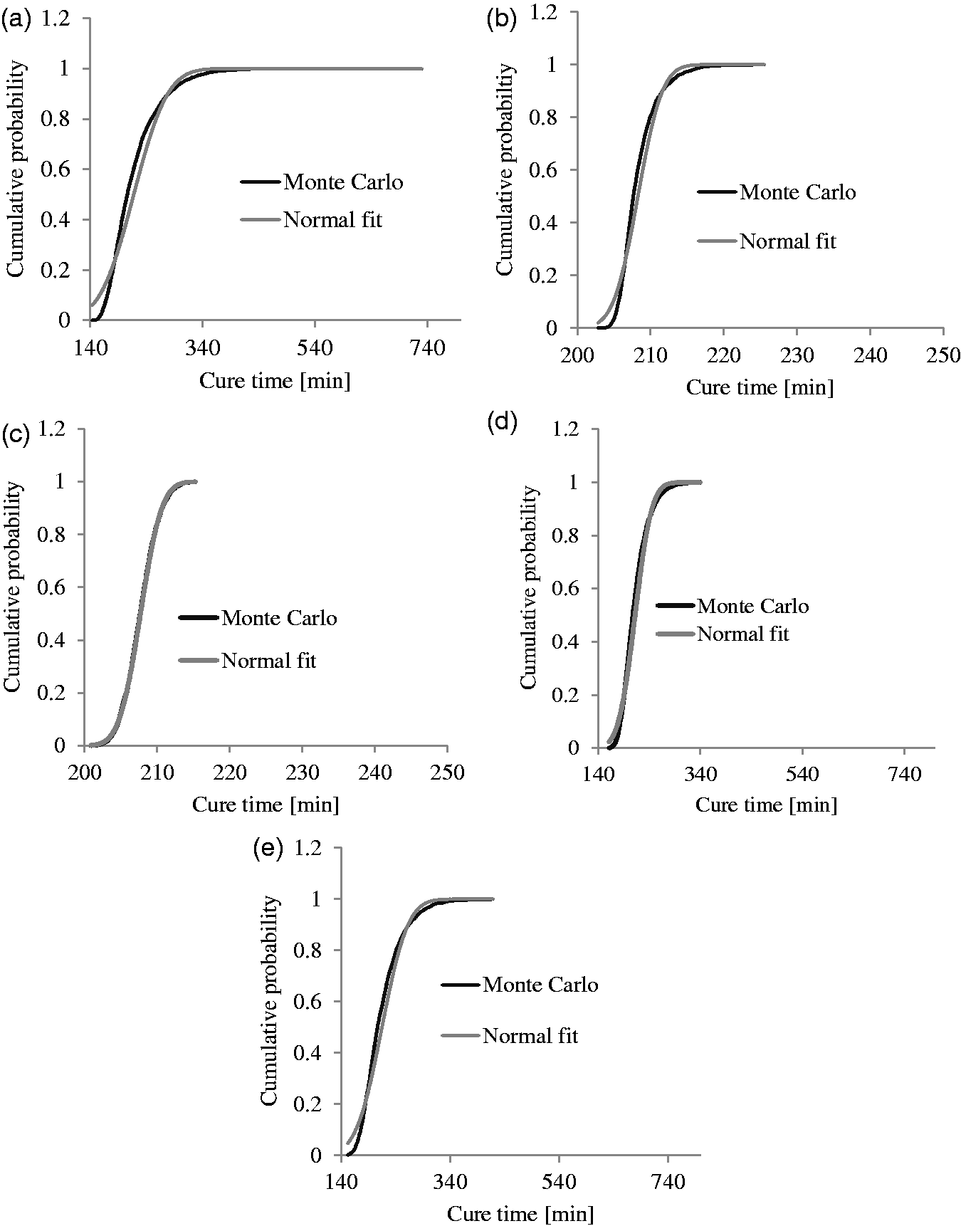

The propagation of variability can be explained considering the heat transfer mechanisms and kinetics followed during the cure. When surface heat transfer coefficient is higher the cure time increases due to heat dissipation on the top of the laminate. In the case of tool temperature variability, higher values of tool temperature result in higher reaction rate which in turn lead to lower cure times. The same behaviour can be observed with ambient temperature due to the fact that higher values of ambient temperature lead to lower natural air convection resulting in lower cure times. In the case of cure kinetics uncertainty low initial degree of cure and low activation energy result in a shift to the peak of reaction to lower times leading to lower cure times.

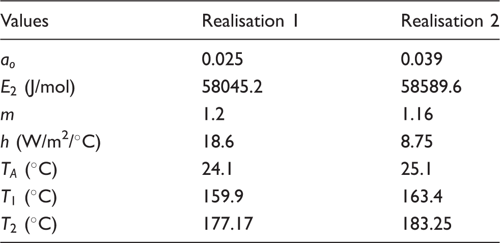
Figure 15 illustrates the evolution of cure reaction rate with time for two realisations of the stochastic simulation model considering the combined effect of boundary conditions and cure kinetics uncertainty and for the deterministic model. The two stochastic cases reported represent the extremes of maximum and minimum cure time. Table 6 reports the values of the stochastic parameters for the two realisations. In realisation 1 (maximum cure time), the cure reaction rate has lower peak values throughout the thickness of the laminate with the peak of reaction at the top of the laminate shifted considerably towards higher times leading to longer cure time. This due to the high surface heat transfer coefficient, low tool temperature and low initial degree of cure values corresponding to this realisation. In contrast, in the case of realisation 2 (minimum cure time), the reaction starts considerably earlier and the peak is higher than the other two cases. Furthermore, the time lag of the onset of reaction between the lower side and the top of the laminate is significantly lower for minimum cure time case (realisation 2). This behaviour can be explained by the low surface heat transfer coefficient, high tool temperature and high initial degree of cure of this realisation (Table 6).

Figure 15.

Evolution of cure reaction rate as a function of time through the thickness of the laminate.

Table 6.

Values of stochastic parameters for two realisations of stochastic model.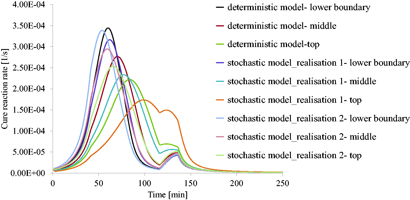

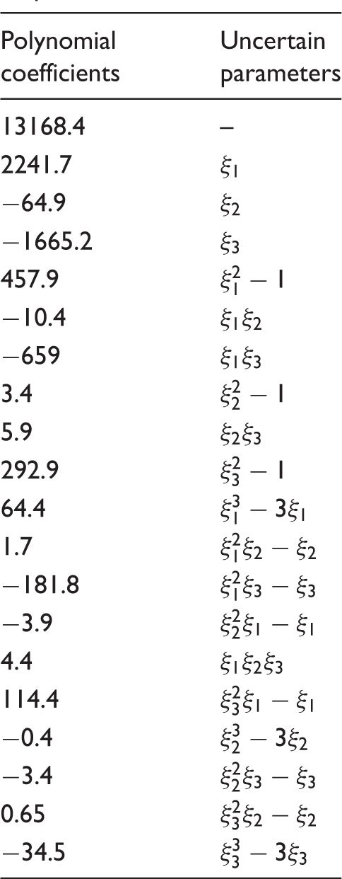
Values	Realisation 1	Realisation 2
a_o	0.025	0.039
E₂ (J/mol)	58045.2	58589.6
m	1.2	1.16
h (W/m²/℃)	18.6	8.75
T_A (℃)	24.1	25.1
T₁ (℃)	159.9	163.4
T₂ (℃)	177.17	183.25

Surface heat transfer coefficient and tool temperature uncertainty dominate cure time variability explaining more than 90% of the overall variability. Therefore, for carbon/epoxy composites stochastic simulation can be limited to these two factors when efficiency is important, e.g. in iterative use. In addition, utilisation of a surrogate model based on PCM can reduce execution times further. This scenario is tested here with the simulation of surface heat transfer and tool temperature variability propagation using both MC and PCM. The third order response surface expressing the cure time as a function of three standard normal variables

ξ_{1}

ξ_{2}

and

ξ_{3}

which represent the three stochastic parameters (h, T₁, T₂) is reported in Table 7.

Table 7.

Third order response surface of cure time.

Polynomial coefficients	Uncertain parameters
13168.4	–
2241.7	$ξ_{1}$
−64.9	$ξ_{2}$
−1665.2	$ξ_{3}$
457.9	$ξ_{1}^{2} - 1$
−10.4	$ξ_{1} ξ_{2}$
−659	$ξ_{1} ξ_{3}$
3.4	$ξ_{2}^{2} - 1$
5.9	$ξ_{2} ξ_{3}$
292.9	$ξ_{3}^{2} - 1$
64.4	$ξ_{1}^{3} - 3 ξ_{1}$
1.7	$ξ_{1}^{2} ξ_{2} - ξ_{2}$
−181.8	$ξ_{1}^{2} ξ_{3} - ξ_{3}$
−3.9	$ξ_{2}^{2} ξ_{1} - ξ_{1}$
4.4	$ξ_{1} ξ_{2} ξ_{3}$
114.4	$ξ_{3}^{2} ξ_{1} - ξ_{1}$
−0.4	$ξ_{2}^{3} - 3 ξ_{2}$
−3.4	$ξ_{2}^{2} ξ_{3} - ξ_{3}$
0.65	$ξ_{3}^{2} ξ_{2} - ξ_{2}$
−34.5	$ξ_{3}^{3} - 3 ξ_{3}$

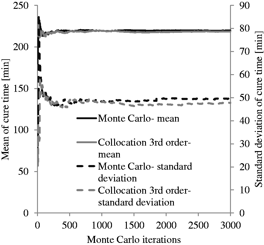
The stochastic simulation results are included in Table 5. Figure 16 illustrates the probability distribution of cure time and Figure 17 presents the convergence of the mean and standard deviation of cure time for the two stochastic simulation schemes. Satisfactory convergence is obtained for the first and second statistical moments of cure time after 1000 Monte Carlo iterations for both stochastic simulation schemes. A very good agreement is achieved between Monte Carlo and the collocation method for the first two statistical moments of cure time. Both stochastic simulation schemes are able to capture the combined effect of surface heat transfer coefficient and tool temperature variability in cure time accurately. The Monte Carlo shows a computationally expensive and rich solution, whereas the PCM offers an efficient approximation with tremendous benefits in terms of computational cost (for the given case, the computational cost of the PCM is 3.9 % of that of the MC), and comparable accuracy.

Figure 16.

Cumulative probability distribution for cure time; surface heat transfer coefficient and tool temperature uncertainty.

Figure 17.

Convergence of statistics of cure time; surface heat transfer coefficient and tool temperature uncertainty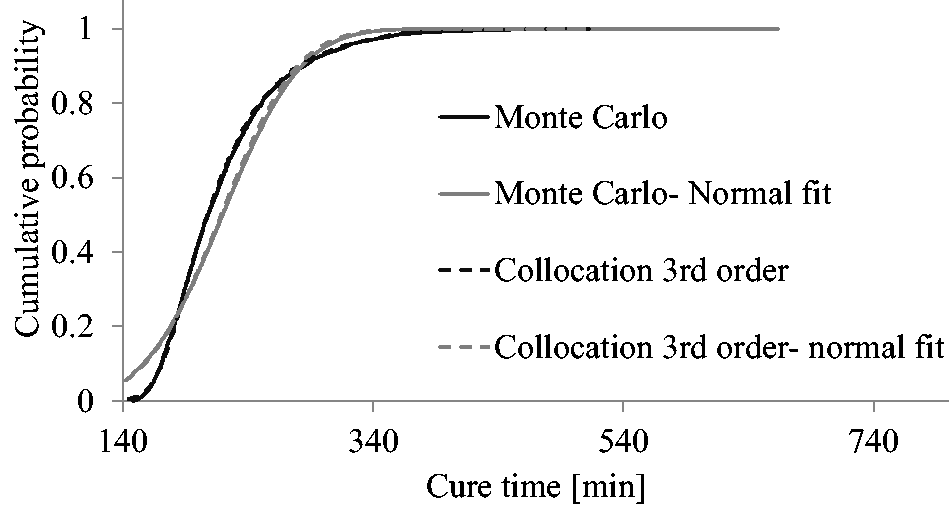

Concluding remarks

The methodologies developed in this study allow the quantification of the influence of boundary conditions variability, cure kinetics uncertainty and their combined effect on the cure process outcome during resin infusion processes. The experimental results show that boundary conditions can show considerable variability, which in turn can introduce significant variation to the process outcome. It is found that the main source of uncertainty in boundary conditions is caused by variation in level across different runs. The stochastic cure simulation results taking into account level variability suggest that surface heat transfer coefficient and tool temperature dominate cure time variability introducing a coefficient of variation of about 22%, with considerable implications in cost associated with process duration and part quality. Cure kinetics and ambient temperature variations introduce negligible variability in cure time in the case of thin high specification epoxy carbon fibre composites. Variations over time introduce negligible variability in cure time in this type of application; however, the effect of variability over time could be significant in which variations in surface heat transfer coefficient and tool temperature are more pronounced (e.g. wind turbine blade manufacturing).

The results of this study show that even in the case of controlled lab conditions where variability is less pronounced than real life applications where less controlled lab conditions are applied and complex geometries can introduce additional variability, variability in boundary conditions can introduce significant variability to the process outcome. Overall, the modelling approaches demonstrated in this study is a powerful tool to characterise and model boundary conditions uncertainty as well as cure kinetics variability in industrial scale applications and investigate its influence on heat transfer effects and residual stress formation during the cure process. Incorporation of variability in process design can contribute towards the optimisation of the process inducing significant benefits in terms of cost by minimising variability in cure time and process defects such as under cure, severe temperature overshoots, and shape distortion.

Footnotes

Declaration of Conflicting Interests

The author(s) declared no potential conflicts of interest with respect to the research, authorship, and/or publication of this article.

Funding

The author(s) disclosed receipt of the following financial support for the research, authorship, and/or publication of this article: This work was supported by the Engineering and Physical Sciences Research Council, through the EPSRC Centre for Innovative Manufacturing in Composites (CIMComp: EP/IO33513/1) and the EPSRC Grant RPOACM (EP/K031430/1).

References

Verleye

Lomov

Long

. Permeability prediction for the meso–macro coupling in the simulation of the impregnation stage of resin transfer moulding. Compos Part A 2010; 41: 29–35.

Endruweit

McGregor

Long

. Influence of the fabric architecture on the variations in experimentally determined in-plane permeability values. Compos Sci Technol 2006; 66: 1778–1792.

Endruweit

Long

. Influence of stochastic variations in the fibre spacing on the permeability of bi-directional textile fabrics. Compos Part A 2006; 37: 679–694.

Endruweit

Long

Robitaille

. Influence of stochastic fibre angle variations on the permeability of bi-directional textile fabrics. Compos Part A 2006; 37: 122–132.

Skordos

Sutcliffe

MPF

. Stochastic simulation of woven composites forming. Compos Sci Technol 2008; 68: 283–296.

Pan

Liang

Zhang

. Statistical characterization of fiber permeability for composite manufacturing. Polym Compos 2000; 21: 996–1006.

Hoes

Dinescu

Sol

. New set-up for measurement of permeability properties of fibrous reinforcements for RTM. Compos Part A 2002; 33: 959–969.

Hoes

Dinescu

Sol

. Study of nesting induced scatter of permeability values in layered reinforcement fabrics. Compos Part A 2004; 35: 1407–1418.

Padmanabhan

Pitchumani

. Stochastic analysis of isothermal cure of resin systems. Polym Comp 1999; 20: 72–85.

10.

Acquah

Datskov

Mawardi

. Optimization under uncertainty of a composite fabrication process using a deterministic one-stage approach. Comput Chem Eng 2006; 30: 947–960.

11.

Mesogitis

Skordos

Long

. Stochastic simulation of the influence of cure kinetics uncertainty on composites cure. Compos Sci Technol 2015; 110: 145–151.

12.

Hexcel®. RTM 6 180℃ epoxy system for resin transfer moulding monocomponent system product data. Available at: www.hexcel.com (2009, accessed 10 November 2014).

13.

HexForce®. G1157 D1300 INJ 2 F carbon fabric. Available at: www.hexcel.com (2013, accessed 10 November 2014).

14.

Marc®. volume D: user subroutines. Available at: www.mscsoftware.com (2011, accessed 10 November 2014).

15.

Karkanas

Partridge

. Cure modeling and monitoring of epoxy/amine resin systems. I. cure kinetics modeling. J Appl Polym Sci 2000; 77: 1419–1431.

16.

Farmer

Covert

. Thermal conductivity of a thermosetting advanced composite during its cure. J Thermophys Heat Transfer 1996; 10: 467–475.

17.

RdF®. HFS-A// heat flux sensors. Available at: http://www.rdfcorp.com (accessed 11 November 2014).

18.

HexTow®. AS7 carbon fiber. Available at: www.hexcel.com (2011, accessed 10 November 2014).

19.

Press

. Numerical recipes: the art of scientific computing, In: Anonymous. 3rd ed. Cambridge, UK: Cambridge University Press, 2007.

20.

Huang

Mahadevan

Rebba

. Collocation-based stochastic finite element analysis for random field problems. Prob Eng Mech 2007; 22: 194–205.

21.

Smith W. On the simulation and estimation of the mean-reverting Ornstein-Uhlenbeck process. Commodities Markets and Modelling, 2010.

22.

Fylstra

Lasdon

Watson

. Design and use of the Microsoft Excel Solver. Interfaces 1998; 28: 29–55.

Stochastic heat transfer simulation of the cure of advanced composites

Abstract

Keywords

Introduction

Methodology

Cure simulation

Experimental setup for the analysis of boundary conditions uncertainty

Stochastic process development

Stochastic simulation approach

Boundary conditions uncertainty

Experimental results

Stochastic processes

Stochastic cure simulation

Short term variability

Effect of level variability across different runs

Concluding remarks

Footnotes

Declaration of Conflicting Interests

Funding

References