Sage Journals: Discover world-class research

Abstract

This study re-examines the validity of Kuznets curve hypothesis for six South Asian countries, namely, Pakistan, Nepal, Bhutan, Sri Lanka, India, and Bangladesh, over the period 1991–2018. The Pooled Mean Group (PMG) technique results in the short and long run reveal an S-shaped curve relationship between income inequality and Gross Domestic Product (GDP) per capita for all countries, that is, negative at the beginning, positive after the first turning point (GDP per capita level, US$473), and negative after the second turning point (GDP per capita level, US$3827) when GDP per capita reaches the maximum level. In contrast, the country-specific results show, that the first and second turning points of GDP per capita are US$468 and US$2298 for India, US$445 and US$1408 for Pakistan, US$450 and US$9045 for Bhutan, and US$925 and US$6836 for Sri Lanka, which support the validity of the S-shaped curve. Moreover, the results also show the existence of N-shaped curve with GDP per capita (i.e. first and second) turning points of US$473 and US$2864 for Bangladesh and US$105 and US$3568 for Nepal. The findings suggest that income inequality gaps in Asian countries seem to be conditional on the levels of GDP per capita. In this regard, expansionary fiscal policy, specifically in the form of government spending, promotion of exports and employment, and price stability can play a vital role in increasing the GDP per capita levels and narrowing the income inequlaity gaps in the selected Asian countries.

Keywords

Gini coefficient Kuznets curve income inequality economic growth S-shaped curve South Asian countries

Introduction

Long-term economic growth and equal distribution of income are considered vital for the economic development and social welfare of the people in a country. The overall effects of economic growth is considered fruitful for a country because on one hand it paves the way for the economic development and contributes toward the social welfare of the people, whereas, on the other hand, it also reflects the overall health economy, at both the domestic and international levels and contributes to the economic development. In contrast to economic growth, income inequality is considered harmful because it slows down the economic growth, results in excessive social conflicts (Wang et al., 2015), and widens the gap between the rich and poor, which ultimately results in deprivation of majority of people from their basic rights. Excessive income inequality can lead to social tensions, for example, higher crime rates, political and economic instability, and poverty (Barro, 2000). In the literature, the pioneered work on the economic growth came upfront from Adam Smith in 1976, whereas the importance of income distribution has been brought to focus by the work of Ricardo (1817).

However, when it comes to the relationship between the economic growth and income inequality, it has received the world’s attention almost more than five decades ago (Shahbaz, 2010) with the introduction of pioneer and influential work done by Simon Kuznet (1955). Kuznet (1955) pointed out that the trend in income inequality and Gross Domestic Product (GDP) per capita resembles an inverted U-shaped pattern. After that, the Kuznets curve hypothesis has been tested and supported by a string of studies conducted for various countries (Angeles, 2010; Bouincha & Karim, 2018; Cheema & Rehman, 2014; Sayed & Peng, 2020), although some of the studies, that is, Robinson (1976) and Anand and Kanbur (1993), did not find any evidence of the Kuznets curve hypothesis.

The South Asian region witnessed an increase in GDP per capita over the last so many years. But this increase in GDP per capita has also been accompanied by of the spread in income inequality. This increase in income inequality and widening gaps between the rich and the poor raised questions on the existence of inverted U-shaped Kuznets curve for these economies. Specifically, during the last three and half decades, in countries like Bangladesh, Pakistan, Sri Lanka, Nepal, and India the increase in GDP per capita is accompanied by a rise in income inequality. However, among the group Bhutan witnessed a decrease in income inequality and a simultaneous increase in GDP per capita, that is, see Table 1 (Solt, 2020; Standardized World Income Inequality Database (SWIID)). This necessitates the needs for further research on the issue for these countries.

Table 1.

GDP per capita and income inequality trends in South Asian regions.

Country	GDP per capita US$ (average values)		Gini (%) (average values)
Country	1980–1999	2000–2018	1980–1999	2000–2018
Pakistan	402	995	35	37
India	357	1188	43	48
Sri Lanka	1286	6697	42	46
Nepal	182	575	40	42
Bhutan	502	2044	45	43
Bangladesh	312	864	37	39

Source. Author’s calculation based on World Development Indicators (WDI) and Solt (2020).

GDP: gross domestic product.

Similarly, Figure 1 depicts the country-wise scatter diagrams showing the relationship between Gini and GDP per capita in linear form over the period 1991–2018. Figure 1 shows that income inequality is the dependent variable measured through Gini coefficient and economic growth is an explanatory variable proxied by GDP per capita. It shows that income inequality widened with the GDP per capita increase for Sri Lanka, Pakistan, Bangladesh, and India. And for Bhutan and Nepal, the Gini and GDP per capita relationship is inverse, showing that the increase in GDP per capita brought decrease in income inequality.

Figure 1.

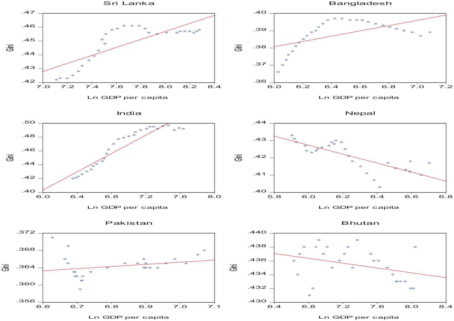
Scattered diagram between Gini and gross domestic product (GDP) per capita for the South Asian Countries.

The Kuznets curve hypothesis states that at the initial stages of development, a country experiences greater levels of income inequality because of lower productivity in the agricultural sector and growing industrial sector. But later on, a decline in the dispersion of wage rate is expected because of a shift of labor from the agricultural sector toward the manufacturing sector and, second, because of the progress in agriculture modernization and productivity (Oczki et al., 2017). Although the Kuznets curve hypothesis has been tested by a large number of studies for both the developed and developing countries, no uniform consensus is available on the existence of U-Kuznets curve in the literature.

Unlike the previous studies, this study provides new insights to the literature by re-examining the validity of the conventional Kuznets curve for six South Asian countries, namely, Sri Lanka, Bangladesh, India, Pakistan, Nepal, and Bhutan. The study is important, in a sense, because against other countries of the world, these countries are having a unique and completely different experience in terms of GDP per capita growth and distribution of income, which invalidate the standard Kuznets curve hypothesis. The increase in GDP or GDP per capita seems not to bring reduction in income inequality in these countries as claimed by Kuznets curve hypothesis. These developments open the room for more research to investigate the relationship between income inequality and economic growth. Moreover, the maximum threshold levels of GDP per capita (i.e. first and second turning points) are empirically estimated, which is another contribution of the study. Finally, latest data series and Pooled Mean Group (PMG) technique application bring more innovation in the overall methodology of the current study.

The main conclusion of the study is, that GDP per capita and inequality relationship are depicting an S-shaped pattern in the selected South Asian countries.

The rest of the study is structured as follows: Section two “Literature review” deals with relevant literature review. Section three “Data and methodology” discusses the data, methodology, and econometric techniques used in the study. After that, section four “Results and discussion” presents the empirical results and its discussion. The final section “Conclusion” represents the conclusion and policy implications.

Literature review

The empirical literature on the relationship between GDP per capita and income inequality is based on Kuznets curve hypothesis. Lin and Weng (2006) empirically tested the Kuznets hypothesis for the East Asian countries. They concluded that Kuznets curve hypothesis remained valid in the context of the East Asian countries. Chambers (2010) conducted a study for 55 developed and developing countries and found that increase in economic growth triggered income inequality in short and medium run in all countries. However, in the long run, economic growth contributes positively to income inequality in developed countries. But in contrast, rising economic growth decreased income inequality in the developing countries. Cheema and Rehman (2014) studied the link between Gini coefficient and per capita GDP for Pakistan economy by utilizing the pooled data spanning from 1993 to 2011. The estimated results of the study were in line with the Kuznets hypothesis. Azam (2019) evaluated the effects of income inequality by regressing inflation, foreign direct investment, worker’s remittances, and human capital on economic growth for Asian and Pacific region over a period from 1996 to 2008. He found a significant negative effect of inequality on growth, which suggests that reducing inequality is necessary for achieving higher economic growth. Younsi and Bechtini’s (2020) empirical findings for Brazil, Russia, India, China, and South Africa (BRICS) countries using data over the period 1990–2015 depicted that economic growth and income inequality relationship followed Kuznets inverted U-shaped pattern. Gomez-Leon (2021) utilized social tables and modern household survey data for testing the presence of Kuznets curve in case of Brazil using data from 1850 to 2010. He concluded that Brazil’s income inequality followed a Kuznets curve trend during the selected period. There are very few studies which contradict the original shape of Kuznets curve. Huang et al. (2012) carried out a study for the United States using data for the period 1917–2007. The study rejected the null hypothesis of inverted U or Kuznets curve hypothesis and supported U-shaped pattern in between income inequality and economic development. Kim et al. (2011) rejected the existence of the inverted U-shaped Kuznets curve and proposed a U-shaped relationship between income inequality and economic growth which was developed by conducting a study for 48 states of the United States for the time period from 1945 to 2004.

The most recent study done by Sayed and Peng (2020) found N-shaped Kuznets curve for the United Kingdom, the United States, Germany, and France. Yang and Greaney (2017) used time series data to study the long-run relationship between income inequality and economic growth and found S-shaped Kuznets curve rather than the conventional U-shaped curve in the context of South Korea, Japan, the United States, and China. Shahbaz (2010), Sinha (2004), and Tribble (1999) in their studies supported the S-shaped Kuznets hypothesis. Table 2 represents prior empirical studies carried out for various countries to test the applicability of Kuznets curve hypothesis. The studies mentioned in the table show mixed results, that is, inverted U-shaped, S-shaped, and N-shaped in the context of different economies.

Table 2.

Selected prior empirical studies on testing Kuznets curve for world countries.

Author/s	Periods, country(s); Techniques	Symbols	Regressors	Findings
Sayed and Peng (2020)	1914–2020 UK, USA, France, and Germany Fixed effect, random and interactive fixed effects	INQ	Real GDP per capita, its square, and cube	N-shaped curve
Bouincha and Karim (2018)	1990–2015 189 countries pooled, fixed, and random effects	Gini	GDP per capita constant, unemployment total, labor force, agriculture value added per worker, health expenditure, inflation, population density, and central government debt on total GDP	Inverted U curve
Yang and Greaney (2017)	1960–2014 China, Japan, South Korea, and USA ECM	Gini	Logarithm of GDP per capita, its square, and cube, export (% of GDP), import (% of GDP), trade, primary education, labor force, fertility rate	S-shaped curve
Cheema and Rehman (2014)	1993–2011 Pakistan Random coefficient model	Gini	Per capita consumption and its square	Inverted U curve
Shahbaz (2010)	1971–2005 Pakistan ARDL	Gini	Logarithm of GDP per capita its square, and cube, FDI (% of GDP), unemployment rate, life expectation, remittances (% of GDP)	S-shaped curve
Bhandari et al. (2010)	1987–2006 57 countries Fixed and random effects and Hausman test	Gini	Logarithm of GDP per capita and its square, money supply (% of GDP), trade (% of GDP)	Inverted U curve
List and Gallet (1999)	1961–1992 71 countries pooled OLS, fixed and random effects	Gini	Income, its square, and cube	N-shaped curve

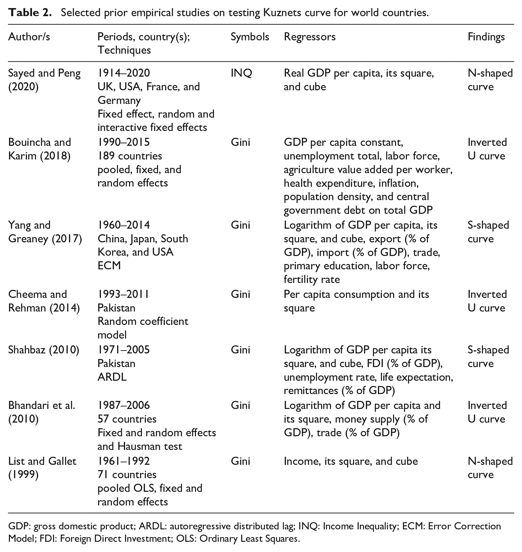
GDP: gross domestic product; ARDL: autoregressive distributed lag; INQ: Income Inequality; ECM: Error Correction Model; FDI: Foreign Direct Investment; OLS: Ordinary Least Squares.

It is evident from the above studies that a series of literature existed on testing the validity of Kuznets curve. But only a small number of empirical studies have been done to test the shape of Kuznets curve. To the best of the authors’ knowledge, this is the first study which uses the latest panel dataset by applying PMG technique to study the income inequality and economic growth relationship for South Asian countries. The study identified and calculated threshold levels of GDP per capita (first and second turning points) for South Asian economies. The study will provide additional empirical evidence on the relationship between GDP per capita and income inequality and to test the validity and shapes of the Kuznets curve in South Asian context.

Data and methodology

The methodology and data information are presented as follows.

Data and its sources

The current study used panel data for six South Asian Countries. The dataset used for analysis is mainly extracted from SWIID (2020) and World Development Indicators (WDI, 2020) for Pakistan, India, Bangladesh, Nepal, Sri Lanka, and Bhutan spanning 1991–2018. Afghanistan and Maldives* are excluded because of non-availability of data. The variables used in the study are given in Table 3.

Table 3.

Description of variables and data sources.

Variables	Symbol	Measurement	Source
Income inequality	Gini	“Based on a Gini Index, it ranges from 0 to 1. Zero indicates perfect income equality while 1indicates perfect income inequality”	SWIID
GDP per capita	Y	“GDP per capita (constant 2010 US$)”	World Development Indicators, World Bank 2021
Exports	EXP	“Exports of goods and services (% of GDP)”
Imports	IMT	“Imports of goods and services (% of GDP)”
Government spending	GS	“General government final consumption expenditure (% of GDP)”
Inflation	INF	“GDP deflator (annual %)”
Labor Force	LF	“Employment to population ratio, 15+, total (%)”
Credit	CRD	Domestic credit provided by financial sector (% of GDP)

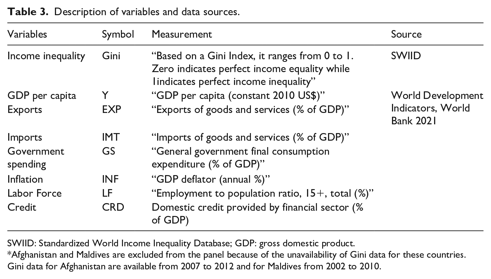
SWIID: Standardized World Income Inequality Database; GDP: gross domestic product.

Afghanistan and Maldives are excluded from the panel because of the unavailability of Gini data for these countries. Gini data for Afghanistan are available from 2007 to 2012 and for Maldives from 2002 to 2010.

It is also important to identify the channels through which GDP per capita affects the income inequality. For this purpose, the following conceptual framework given in Figure 2 has been designed. The figure shows the direct and indirect channels through which income inequality is influenced by economic growth. The direct channel addresses the structural changes because of the growth process that affects the income inequality, whereas social and demographic factors indirectly contribute to income inequality. The direct effects show, that economic growth affects the distribution of income through three channels. First, as defined by Kuznets curve, through the structural transformation from agriculture to manufacturing sector. Second, in the form of capital income, as increase in large capital gains results in increase in the income of elite class that further leads to income inequality. Third, strong economic growth favors the poor masses and decreases income inequality in a form of creating new job opportunities by allowing the low wage workers to move from the informal to the formal labor market. While low level of economic growth exerts downward pressure on the economy and adversely affects the wages of the poor sector, it leads to increase in the income inequality (Yang & Greaney, 2017). Regarding indirect effects, Barro (2000) found that higher educational attainment in the form of human capital leads economies toward more equal income distribution.

Figure 2.

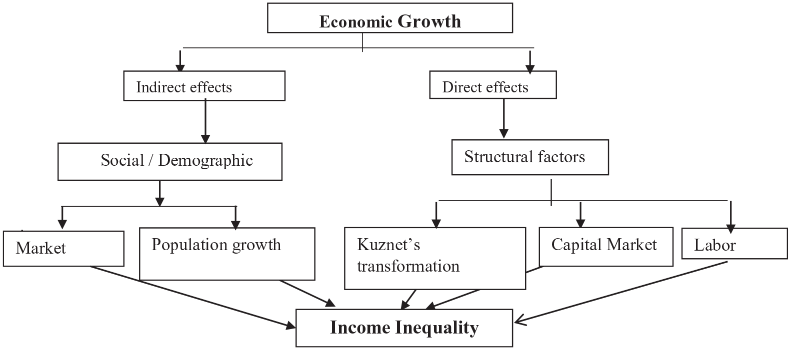
Conceptual framework.

Model specification

The traditional Kuznets curve framework was used by Yang and Greaney (2017), Shahbaz (2010), and List and Gallet (1999). According to the Kuznets (1955) and Ahluwalia (1976), the role of economic growth in income inequality is represented by GDP per capita. A priori nonlinear relationship between per capita GDP and income inequality emerged in line with this argument. This paper models Gini coefficient in a cubic polynomial function of per capita GDP as follows.

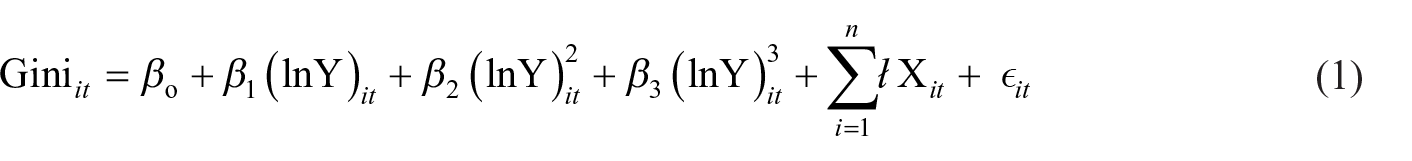
{G i n i}_{i t} = β_{o} + β_{1} {(l n Y)}_{i t} + β_{2} {(l n Y)}_{i t}^{2} + β_{3} {(l n Y)}_{i t}^{3} + \sum_{i = 1}^{n} ø X_{i t} + ϵ_{i t}

(1)

where in equation (1) the term Gini_it is the measure for income inequality, the independent variable (lnY)_it is a symbol used for GDP per capita_it and is expressed in natural logarithm form, while ${(l n Y)}_{i t}^{2}$ and ${(l n Y)}_{i t}^{3}$ are used as symbols for square (lnGDP per capita_t)² and cubic (lnGDP per capita_t)³, respectively.

In the equation if β₁ < 0, β₂ > 0, β₃ < 0, the GDP per capita and income inequality relationship will reveal an S-shaped curve. In contrast, if β₁ > 0, β₂ < 0, β₃ > 0, it will reflect the existence of N-shape.

The square ln GDP per capita has been included in the equation to test the conventional Kuznets curve. This (ln GDP per capita)² basically represents the idea that initially the income inequality increases with the increase in GDP per capita. However, later on, after the transformation of the economy with the transition from becoming more dependent on the manufacturing sector against the agriculture sector representing the first turning point, the income inequality decreases with the increase in GDP per capita depicting a U-shaped Kuznets curve. Moreover, the cubic ln GDP per capita represents the extension of the traditional Kuznets curve, depicting the transformation of the economies, becoming more dependent on the services sector in contrast to the manufacturing sector, extending the inverted U-shaped curve and depicting an S-shaped (Sinha, 2004; Tribble, 1999) or N-shaped curve for most of the countries (List and Gallet, 1999) revealing the second turning point. The turning points explain the income inequality trends before and after the turning points. The exclusion of the cubic form of (ln GDP per capita)³ from the GINI equation may lead to model misspecification as most of these countries are now dependent heavily on the services sector along with the other two sectors.

The term X_it shows all other explanatory variables used in the model, ∅ represents the relevant coefficients, and ϵ_it is the error term and i = country, t = time.

X(it) is vector for six additional variables. The first variable is the employment to population ratio used as an indicator for labor force/labor market conditions (Censky, 2012). The second variable is government expenditure which is a percentage of GDP, to measure the relative size of each country’s spending (Yang and Greaney, 2017). Third and fourth variables are export and import as ratio to GDP, respectively. The fifth variable is GDP deflator, a proxy for inflation (Jiang et al., 2011). And sixth is the measure for financial sector represented by domestic credit percentage of GDP (Gonzalez and Resosudarmo, 2018).

In their studies, Yang and Greaney (2017) and Shahbaz (2010) used (ln GDP per capita), (ln GDP per capita)², and (lnGDP per capita) as proxies for economic growth by finding S-shaped curve.

Equation (1) provides the empirical characteristics of β₁, β₂, and β₃ showing the shapes of Kuznets hypothesis for testing several forms of economic growth–income inequality relationship (Clance et al., 2019). (a) β₁ > 0, β₂ = β₃ = 0 implies an increasing linear relationship, which means that increasing levels of inequality are accompanied by rising incomes; (b) β₁ < 0, β₂ = β₃ = 0 reveals a decreasing linear function; (c) β₁ > 0, β₂ < 0, and β₃ = 0 indicates a quadratic relationship in an inverted U-shaped pattern; (d) β₁ < 0, β₂ > 0, and β₃ = 0 reveals a quadratic relationship in U-shaped pattern, in direct contrast with Kuznets curve; (e) β₁ > 0, β₂ < 0, β₃ > 0 reveals an N-shaped curve; (f) β₁ < 0, β₂ > 0, β₃ < 0 suggests an S-shaped function; and (g)β₁ = β₂ = β₃ = 0 indicates a flat behavior (Figure 3)

Figure 3.

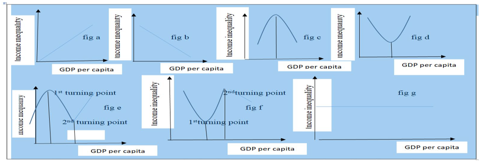
Kuznets curve pattern for the relationship between income inequality and economic growth.

GDP per capita threshold levels

In this study, I used a balanced dataset to evaluate the nonlinear relationship hypothesis between the Gini coefficient and the per capita GDP threshold level. I have used the method of Onafowora and Owoye (2014: 50) and Yang et al. (2010: 67) to estimate the first and second turning points of the GDP per capita threshold level. This threshold level is measured by using the coefficients of GDP per capita, its square, and cube, which is given by

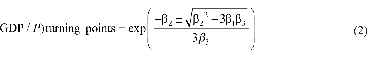
G D P / P) t u r n i n g p o i n t s = e x p (\frac{- β_{2} \pm \sqrt{{β_{2}}^{2} - 3 β_{1} β_{3}}}{3 β_{3}})

(2)

where GDP divided by population represents GDP per capita. And the terms β₁, β₂, and β₃ are coefficients in natural logarithmic form for GDP per capita, its square, and cube, respectively.

The PMG application

Pesaran et al. (1999) used an innovative co-integration technique by introducing the Autoregressive Distributed Lag (ARDL) in the form of error correction model. They claimed that the panel ARDL model, in particular, the PMG technique, can be employed even for the data with mixed order of integration.

The present study modified and followed the model used by Arnold et al. (2011) with the help of econometric technique panel Error Correction Model (ECM). The model of Pesaran et al. (1999) is also employed byAcosta-Ormaechea et al. (2019), Baiardi et al. (2017), and Azam (2019)

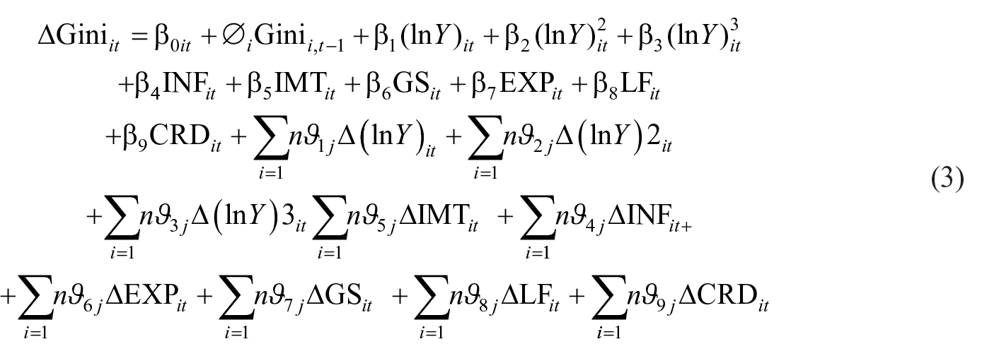
\begin{matrix} Δ {G i n i}_{i t} = β_{0 i t} + \emptyset_{i} {G i n i}_{i, t - 1} + β_{1} {(l n Y)}_{i t} + β_{2} {(l n Y)}_{i t}^{2} + β_{3} {(l n Y)}_{i t}^{3} \\ + β_{4} {I N F}_{i t} + β_{5} {I M T}_{i t} + β_{6} {G S}_{i t} + β_{7} {E X P}_{i t} + β_{8} {L F}_{i t} \\ + β_{9} {C R D}_{i t} + \sum_{i = 1} n ϑ_{1 j} Δ {(l n Y)}_{i t} + \sum_{i = 1} n ϑ_{2 j} Δ {(l n Y) 2}_{i t} \\ + \sum_{i = 1} n ϑ_{3 j} Δ {(l n Y) 3}_{i t} \sum_{i = 1} n ϑ_{5 j} Δ {I M T}_{i t} + \sum_{i = 1} n ϑ_{4 j} Δ {I N F}_{i t +} \\ + \sum_{i = 1} n ϑ_{6 j} Δ {E X P}_{i t} + \sum_{i = 1} n ϑ_{7 j} Δ {G S}_{i t} + \sum_{i = 1} n ϑ_{8 j} Δ {L F}_{i t} + \sum_{i = 1} n ϑ_{9 j} Δ {C R D}_{i t} \end{matrix}

(3)

where,

j and k shows lags of variables (j:1,2…..p; k:1,2,3….q)

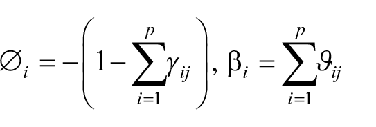
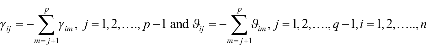
\emptyset_{i} = - (1 - \sum_{i = 1}^{p} γ_{i j}), β_{i} = \sum_{i = 1}^{p} ϑ_{i j}

γ_{i j} = - \sum_{m = j + 1}^{p} γ_{i m}, j = 1, 2, \dots ., p - 1 a n d ϑ_{i j} = - \sum_{m = j + 1}^{p} ϑ_{i m}, j = 1, 2, \dots ., q - 1, i = 1, 2, \dots .., n

and

i = 0,1,2,…,n,∅_i is the correction termfromthe short-run to long-run equilibrium.

Results and discussion

The estimation strategy of the study consists of the following steps. First, Panel Unit Root Tests (PURTs) including Levin, Lin, and Chu (LLC); Im, Pesaran, and Shin (IPS); Augmented Dickey–Fuller (ADF) chi-square are applied to data for checking unit root. The obtained results are given in Table 4 illustrating that the two variables Gini coefficient and inflation are stationary at level. However, GDP per capita, export, import, government spending, labor force, and credit became stationary at the first difference. This dissimilar order of integration of all the variables recommended the application of PMG technique for estimating the results. The PMG technique has been used for computing both the short- and long-run results for the whole panel. Moreover, short-run coefficients are also estimated for all countries individually.

Table 4.

Panel Unit Root Test (PURT) results.

Variables	LLC test		IPS test		ADF chi² test		Decision
Variables	At level	At 1st Dif.	At level	At 1st Dif.	At level	At 1st Dif.
Gini_it	−2.85* (0.00)	−	−1.99** (0.02)	−	20.85 (00.06)	41.55*(0.00)	I (0), I(1)
lnY_it	4.18 (1.00)	−2.34* (0.00)	7.05 (1.00)	−3.37* (0.00)	0.37 (1.00)	39.27* (0.00)	I(1)
(lnY_it)²	4.94 (1.00)	−1.83** (0.01)	7.47 (1.00)	−3.23* (.003)	0.20 (1.00)	34.70* (0.00)	I(1)
(lnY_it)³	5.63 (1.00)	−2.82** (0.04)	8.28 (1.00)	−3.81* (0.00)	0.11 (1.00)	36.19* (0.00)	I(1)
INF_it	−1.78** (0.03)	−	−2.49* (0.00)	−	27.71* (0.00)	−	I(0)
IMT_it	−0.42 (0.33)	−6.88* (0.00)	−0.21 (0.41)	−6.57* (0.00)	9.94 (0.61)	63.57* (0.00)	I(1)
GS_it	−0.34 (0.55)	−7.05* (0.00)	−0.73 (0.31)	−7.12* (0.00)	14.53 (0.36)	69.62* (0.00)	I(1)
EXP_it	0.50 (0.69)	−2.17** (0.01)	0.87 (0.81)	−4.74* (0.00)	7.29 (0.83)	44.68* (0.00)	I(0)
LF_it	−0.96** (0.02)	−	0.85 (0.80)	−4.20* (0.00)	6.06 (0.91)	43.51* (0.00)	I(0), I(1)
CRD_it	0.36 (0.64)	−4.51* (0.00)	2.25 (0.98)	−5.48* (0.00)	4.56 (0.97)	52.89* (0.00)	I(1)

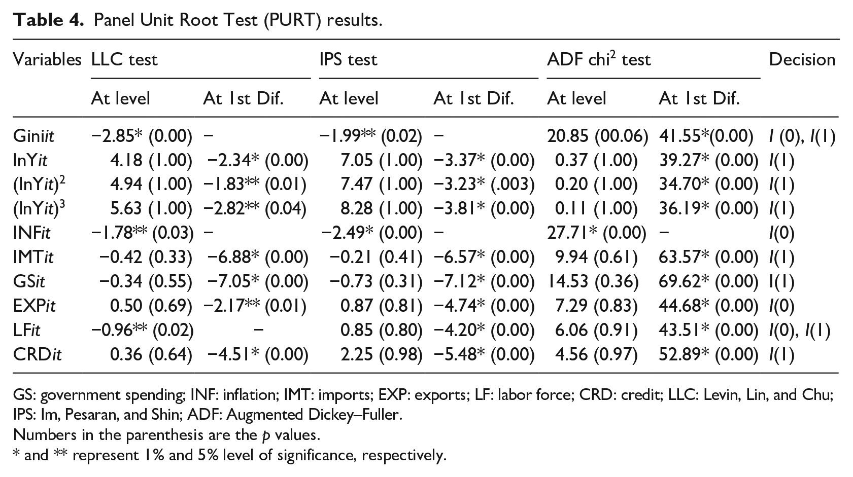
GS: government spending; INF: inflation; IMT: imports; EXP: exports; LF: labor force; CRD: credit; LLC: Levin, Lin, and Chu; IPS: Im, Pesaran, and Shin; ADF: Augmented Dickey–Fuller.

Numbers in the parenthesis are the p values.

and ** represent 1% and 5% level of significance, respectively.

Table 5 presented the descriptive statistics and correlation matrix results. The results are computed for the full panel of South Asian countries. The descriptive statistics findings show that the maximum value of Gini is recorded to be 0.47, while its minimum value is 0.35 during the study period. The mean of Gini, (lnY), INF, IMT, GS, EXP, LF, and CRD are recorded as 0.42, 6.91, 7.49, 30.61, 10.82, 20.85, 59.87, and 46.96, respectively, and the standard deviations are 0.03, 0.59, 4.29, 14.86, 4.55, 10.33, 11.70, and 18.02, respectively. All variables are normally distributed as the skewness values lie between −1.96 and 1.96. Moreover, the negatively skewed variables are INF and CRD. However, Gini, GDP per capita, IMT, GS, EXP, and LF show positive skewness. The values of Kurtosis for all variables are positive and show normal distribution. Furthermore, the correlation coefficient values for all variables including Gini, (lnY), INF, IMT, GS, EXP, LF, and CRD are 0.47, −0.12, 0.37, 0.31, 0.44, 0.06, and 0.18, respectively.

Table 5.

Descriptive statistics summary and correlation matrix results.

	Gini	(lnY _it)	(lnY _it)²	(lnY_it)³	INF_it	IMT_it	GS_it	EXP_it	LF_it	CRD_it
Mean	0.42	6.91	48.23	338.78	7.49	30.61	10.82	20.85	59.87	46.96
Median	0.42	6.84	46.88	321.04	6.98	27.88	10.30	17.69	54.69	46.62
Maximum	0.47	8.28	68.56	567.75	24.89	72.44	22.70	56.27	84.69	85.96
Minimum	0.35	5.90	34.87	205.97	1.13	8.49	4.13	6.66	47.56	−1.30
SD	0.03	0.59	8.38	89.36	4.29	14.86	4.55	10.33	11.70	18.02
Skewness	0.01	0.41	0.57	0.72	−1.26	0.82	0.95	1.01	1.136	−0.26
Kurtosis	2.23	2.40	2.55	2.76	5.45	2.95	3.43	3.57	2.84	3.02
Jarque-Bera	4.14	7.36	10.50	15.10	87.27	18.88	26.74	31.01	35.24	1.96
Gini_it	1
(lnY_it)	0.47	1
(lnY_it)²	0.47	0.99	1
(lnY_it)³	0.48	0.99	0.99	1
INF_it	−0.12	−0.06	−0.06	0.07	1
IMT_it	0.37	0.48	0.48	0.48	−0.01	1
GS_it	0.31	0.44	0.43	0.41	0.01	0.73	1
EX_it	0.44	0.55	0.55	0.54	−0.01	0.83	0.65	1
LF_it	0.06	−0.44	−0.42	−0.41	−0.02	0.37	0.17	0.04	1
CRD_it	0.18	0.24	0.24	0.23	−0.05	−0.21	−0.21	−0.32	−0.17	1

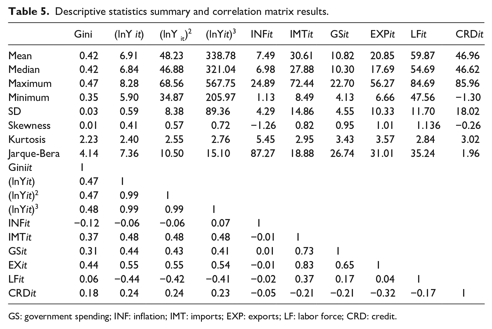
GS: government spending; INF: inflation; IMT: imports; EXP: exports; LF: labor force; CRD: credit.

Table 6 presents that due to a low value of Akaike information criteria, model with a lag length (1, 1, 1, 1, 1, 1, 1, 1, 1, 1) is selected.

Table 6.

Lag length selection criteria.

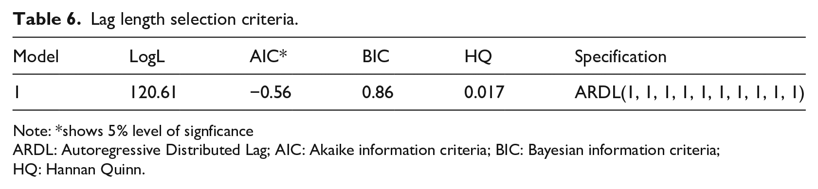
Model	LogL	AIC*	BIC	HQ	Specification
1	120.61	−0.56	0.86	0.017	ARDL(1, 1, 1, 1, 1, 1, 1, 1, 1, 1)

Note: *shows 5% level of signficance

ARDL: Autoregressive Distributed Lag; AIC: Akaike information criteria; BIC: Bayesian information criteria; HQ: Hannan Quinn.

The long-run and short-run results for the full panel are computed through PMG technique. The long-run results given in Table 7 show that the coefficients of GDP per capita, GDP per capita square, and GDP per capita cube turned significant with negative, positive, and negative signs, respectively. These results indicate that the income inequality and GDP per capita relationship followed an S-shaped curve pattern and nullified the existence of inverted U-shaped hypothesis for the Asian countries. One possible argument for this S-shaped pattern can be that the Kuznets curve is not covering the second transition of the economies from the manufacturing sector to services sector which only focuses on the first transition from agricultural sector to manufacturing sector. The second transition is covered by the S-curve. The S-shaped relationship is not new, and many other research already found this shape in the case of various developed and developing countries. For example, (see, Sinha, 2004; Yang and Greaney, 2017). Other variables also turned significant. Inflation exhibited positive and significant relationship with income inequality, which means that the increase in inflation because of rising cost of living and decrease in purchasing power, pressing the poor and making them more poorer, widen the income inequality of the poor class against the rich (Destek et al., 2020; Thalassinos et al., 2012). Imports also became negative in widening the income inequality. This increase in ratio of imports of GDP means leakages of foreign reserves, putting worse effects on the domestic industries, employment, and prices, leading to government spending remaining inversely related to income inequality. This shows that expansionary fiscal policy measures in the form of the increase in government spending can play an instrumental role in narrowing the widening gap of income inequality. Similarly, exports also turned negatively significant, reflecting that increase in share of GDP minimizes disparities in income inequality because of its positive impacts on domestic production, investment, and employment. It has also been noticed that government spending in the form of developmental projects and more spending on lower or middle classes creates more jobs opportunities for the people, specifically for the poor (Claus et al., 2014; Martinez-Vasquez et al., 2012). Similarly, labor force coefficient also showed negative association with Gini coefficient. This increase in labor force and employment is also important for more equal distribution of income in a country (Asteriou et al., 2014). The sign of credit provided by financial sector to Gini is positive and significant, which shows that the financial sector only benefits the rich and can increase income inequality. These results are consistent with findings of Fowowe and Abidoge (2013), Jauch and Watzka (2016), and Wahid et al. (2011).

Table 7.

PMG Long run and short run results for full panel.

Dependent variable: income inequality
Variables	Coefficient	SE	t-statistic	Prob.*
Long-run equation
(lnY_it)	−6.09***	1.242763	−4.9056	0.0000
(lnY_it)²	0.87***	0.175671	5.0045	0.0000
(lnY_it)³	−0.04***	0.008241	−5.0674	0.0000
INF_it	0.01**	0.000295	2.1367	0.0356
IMT_it	0.001***	0.00045	3.6176	0.0005
GS_it	−0.002***	0.000792	−3.2874	0.0015
EXP _it	−0.001***	0.000426	−4.0764	0.0001
LF_it	−0.001**	0.000788	−2.3637	0.0199
CRD_it	0.0004***	0.000119	4.1773	0.0001
Short-run equation
D(lnY_it)	−10.3073	10.35764	−0.99514	0.3223
D(lnY_it)²	1.437696	1.511041	0.95146	0.3438
D(lnY_it)³	−0.06714	0.073405	−0.91467	0.3627
D(INF_it)	−0.00215	0.000115	−1.32218	0.1894
D(IMP_it)	0.000467	0.00035	1.335871	0.1849
D(GS_it)	0.0006***	0.00026	3.10039	0.0026
D(EXP _it)	−0.0008	0.00047	−1.15816	0.2498
D(LF_it)	−0.00073	0.0015	−0.48829	0.6265
D(CRD_it)	0.00068	0.0095	0.040198	0.968
C	3.74009	1.8291	2.044059	0.0438
ECM	−0.25***	1.125936	−4.04547	0.0046

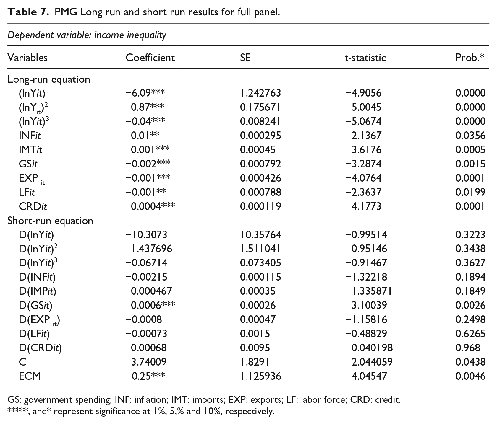
GS: government spending; INF: inflation; IMT: imports; EXP: exports; LF: labor force; CRD: credit.

***

**, and* represent significance at 1%, 5,% and 10%, respectively.

Table 7 also showed the PMG short-run results. It is found that all of the variables turned insignificant in the short run except government spending which became significant but with a positive sign. However, the signs of GDP per capita, its square, and cube depicted an S-shape for the Asian economies also in the short run. The ECM coefficient remained negative and significant. The value of the speed of adjustment parameter is −0.25. This means that the short-term deviation of income inequality will be corrected with a speed of 25.32%in the long run.

Figure 4 shows the relationship between Gini coefficient and GDP per capita. The empirical findings of the S-shaped curve shows that income inequality is increasing in between first (GDP per capita US$473.42) and second turning points (GDP per capita US$3827.26)*.

Figure 4.

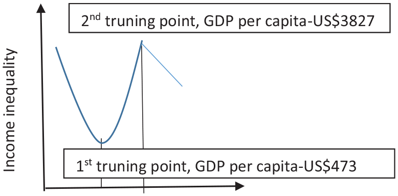
Gini coefficient and gross domestic product (GDP) per capita relationship.

Table 8 shows the short-run results along with the GDP per capita turning points for each country separately. The findings reveal that GDP per capita and Gini relationship showed an S-curve pattern for the countries including Sri Lanka, India, Pakistan, and Bhutan. For all countries, the signs of the coefficients of log GDP per capita, log GDP per capita square, and cube of log GDP per capita are negative, positive, and negative, respectively. These results exhibit that GDP per capita and Gini relationship follow an S-shaped pattern. The S-curve results are in line with the findings of Yang and Greaney (2017) who reached to a similar conclusion for four economies including China, Japan, South Korea, and the United States. Moreover, in case of Sri Lanka, India, and Bhutan, the log GDP per capita remained insignificant, whereas log GDP per capita, square, and cube turned significant. However, for Pakistan, the log GDP per capita remained insignificant in all three forms. These results still supported the S-curve.

Table 8.

PMG short-run results for individual countries.

Dependent variable: income inequality
Variables/Countries	Sri Lanka	Bangladesh	India	Nepal	Pakistan	Bhutan
Δ (lnY_t)	−18.18(20.47)	14.08* (5.70)	−57.15(79.47)	5.41(572.88)	−0.50(846.10)	−5.50(10.88)
Δ(lnY_t)²	2.35*** (0.35)	−2.12(0.13)	8.34*** (1.67)	− 0.79(14.31)	0.11(18.11)	0.72* (0.20)
Δ(lnY_t)³	−0.10*** (0.00)	0.10*** (0.00)	−0.40*** (0.00)	0.03(0.03)	−0.008(0.04)	−0.03*** (0.00)
Δ(INF_t)	− 2.33*** (0.0046)	−0.001*** (0.00017)	0.0007*** (0.0046)	0.000419*** (0.000366)	0.003*** (0.00099)	0.00693*** (0.003)
Δ(IMT_t)	−0.0007*** (0.000701)	−0.004** (0.000322)	0.002*** (0.000019)	0.0001*** (0.0000253)	−0.00074***(0.0000128)	−0.0001*** (0.000619)
Δ(GS_t)	0.004*** (0.00015)	0.004*** (0.000089)	−0.005*** (0.000677)	0.0001*** (0.000143)	0.00314*** (0.000064)	0.0002*** (0.0000349)
Δ(EXP_t)	−0.00048*** (0.0000187)	−0.0083*** (0.000372)	−0.002*** (0.000019	−0.002*** (0.000226)	−0.00714*** (0.000539)	0.00688*** (0.000939)
Δ(LF_t)	−0.00075*** (0.00003)	0.0006*** (0.000145)	0.003*** (0.00025)	−0.00038*** (0.000546)	−0.001873*** (0.000027)	−0.0003*** (0.000018)
Δ(CRD_t)	−0.00058*** (0.56)	−0.00057*** (0.000285)	0.0001*** (0.000418)	−0.06*** (0.0000444)	0.00096*** (0.000068)	0.0001*** (0.000044)
ECM	−0.17*** (0.00)	−0.03*** 0.00	−0.68*** (0.01)	−0.59* (0.03)	−0.14*** (0.001)	−0.02*** (0.001)
First turning points	US$925	US$473	US$468	US$105	US$445	US$450
Second turning points	US$6836	US$2864	US$2298	US$3568	US$1408	US$9045

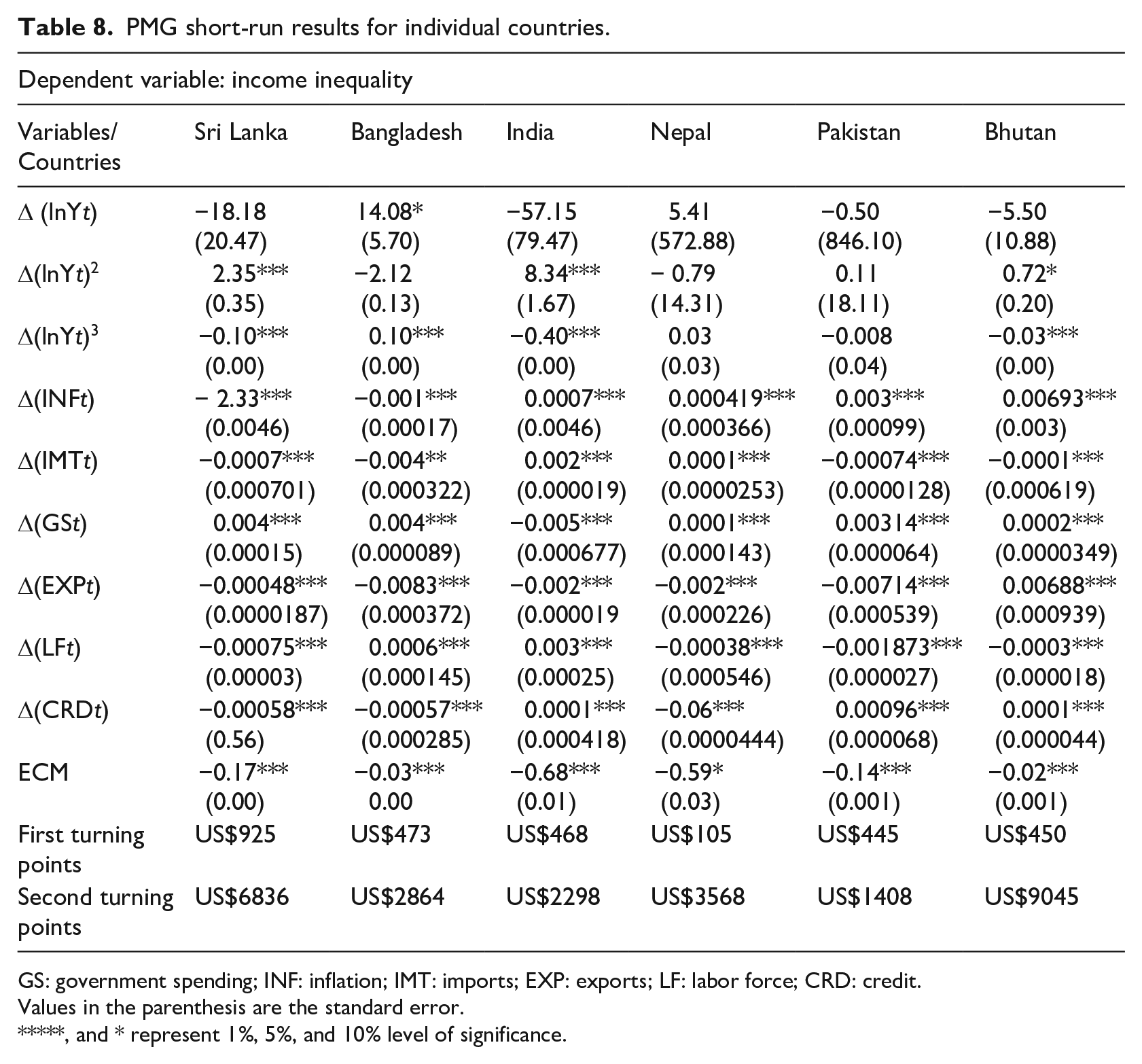
GS: government spending; INF: inflation; IMT: imports; EXP: exports; LF: labor force; CRD: credit.

Values in the parenthesis are the standard error.

***

**, and * represent 1%, 5%, and 10% level of significance.

In contrast, the log GDP per capita and Gini relationship showed N-curve pattern for Bangladesh and Nepal. The signs of the coefficient of log GDP per capita, square, and cube remained positive, negative, and positive. The N-curve that was initially showing inequality increases and then decreases, and after a certain point, it again starts to increase. The N-shaped curve results are in line with the studies of List and Gallet (1999) and Sayed and Peng (2020). However, in case of Bangladesh, log GDP per capita and its cube remained significant. And log GDP per capita square turned insignificant, whereas for Nepal all forms of log GDP per capita remained insignificant.

In case of all countries, the GDP per capita remained insignificant in one or another form. However, its signs are in line with the S-curve or N-curve hypothesis. Similar results are also obtained by Yang and Greaney (2017) for S-curve and Sayed and Peng (2020) for N-curve.

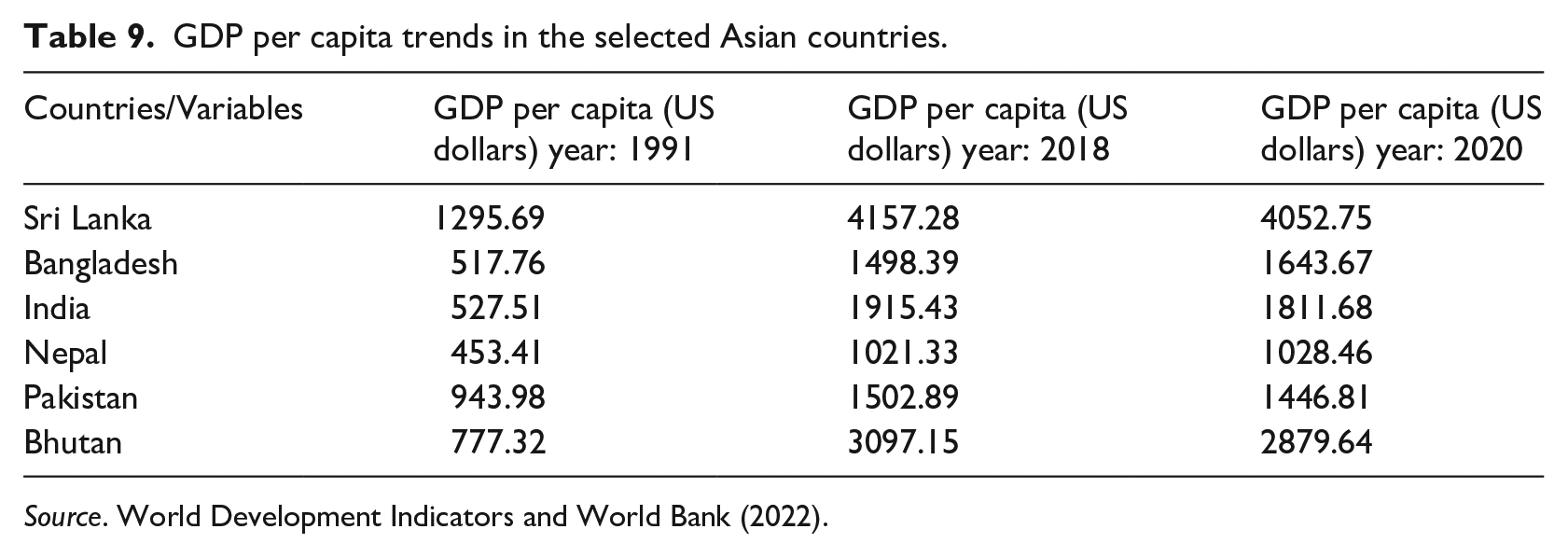
The first and second turning points of GDP per capita for Sri Lanka (US$925, US$6836), Bangladesh (US$473, US$2864), India (US$468, US$2298), Nepal (US$105, US$3568), Pakistan (US$445, US$1408), and Bhutan (US$450, US$9045) are found. These results revealed different turning points (i.e. first and second) and upward trend in GDP per capita for each country. However, Pakistan, Sri Lanka, India, and Bhutan experienced reduction in inequality after the second turning point (i.e. with the increase in GDP per capita), whereas Bangladesh and Nepal case shows widening of income inequality after the second turning point. The GDP per capita details are presented for the years 1991, 2018, and 2020, which clearly show the variations in all countries in the GDP per capita (i.e. Table 9, Appendix 1). As shown in Tables 8 and 9, countries with a low GDP per capita were having lower levels of first and second turning points and countries with a high GDP per capita were having greater turning points.

Nepal’s GDP per capita remained lowest in the group during the years 1991, 2018, and 2020 with GDP per capita levels of US$453.41, US$1021.33, and US$1028.46, respectively. That is the reason that its first turning point (i.e. US$105) remained lowest against other countries. Similarly, Pakistan’s first and second turning points also remained smaller (i.e. US$445 and US$1408) and the reason is its low levels of GDP per capita in given years (US$943.98, US$1502.89, and US$1446.81). Sri Lanka’s GDP per capita remained high (i.e. US$1295.69, US$4157.28, and US$4052.75) during 1991, 2018, and 2018 as compared to other countries. And its first (US$925) and second (US$6836) turning points are also high against other countries in the group. However, its second turning point value is less than Bhutan (US$9045). Bhutan GDP per capita also remained high in the years 1991, 2018, and 2018 (i.e. US$777.32, US$3097.15, and US$2879.64). Because of this reason, its second turning point (US$9045) is greater against all countries in the group. Furthermore, India and Bangladesh turning points are also smaller against other countries except Pakistan. And the reason is the countries’ lower levels of GDP per capita.

Overall, the possible explanations for the differences in the first and second turning points of all the countries are the differences in the per capita GDP. Moreover, these differences also reflect the differences in the countries’ characteristics in terms of economic conditions and policies, the process and speed of transition from agricultural to manufacturing, and further transition to services sectors. Finally, the income inequality (i.e. Gini values) levels and increasing and decreasing rates of one country’s turning point are also different from each other.

The results for other control variables show that inflation remained significant for all countries but with positive signs for India, Nepal, Pakistan, and Bhutan and negative signs for Sri Lanka and Bangladesh. Imports turned positively significant in case of India and Nepal and negatively significant for other countries. Government spending was significant with a negative sign in case of India and positive sign for other countries. Exports are significant with negative signs for all countries except Bhutan for which it is positively significant. Labor force turned negatively significant for all countries, except Bangladesh and India for which it became positively significant. Credit shows mixed results for all countries.

The findings show that inflation and imports are harmful for income inequality. And increase in exports and labor force results in contraction of income inequality in most of the countries.

Conclusion and policy implications

This study re-examined the GDP per capita and income inequality relationship for selected South Asian countries over the period 1991–2018. The PMG short- and long-run results revealed an S-curve pattern and invalidated the inverted U-shaped Kuznets hypothesis for Asian countries. The relationship between income inequality and GDP per capita showed a negative trend at the beginning, positive after the GDP per capita’s first turning point and negative after the second turning point, when GDP per capita reached a maximum level. The GDP per capita threshold levels (i.e. the first and second turning points) were US$473.42 and US$3827.26, respectively. In contrast, the individual countries’ short-run results showed that the GDP per capita first and second turning points were US$468 and US$2298 for India, US$445 and US$1408 for Pakistan, US$450 and US$9045 for Bhutan, and US$925 and US$6836 for Sri Lanka. However, showing N-shaped pattern, the first and second turning points for Bangladesh were US$473 and US$2864 and in case of Nepal were US$105 and US$3568. Among the other variables, government spending, exports, employment, and inflation also turned significantly important in the determination of income distribution in South Asia.

On the basis of the findings, this study proposed a number of policy suggestions for tackling income inequality in South Asian. First, the S-shaped relationship between the income inequality and GDP per capita in the regions collectively and Pakistan, India, Sri Lanka, and Bhutan at individual levels showed that the governments steps for boosting up the GDP per capita levels are important in reducing the spread in income inequality. Moreover, the N-shaped curve detection for Bangladesh and Nepal is showing that the GDP per capita increase is not pro-poor and most of the benefits are received by the rich, resulting in widening of the income inequality gap despite the GDP per capita increase. The findings highlighted the fact that effective and pro-poor policies are required for increasing the GDP per capita, which could be helpful in lowering the income inequality in South Asia. Some of the measures as suggested by the findings of the study might be the increase in government spending, exports, and employment and keeping inflation in control in the region.

Footnotes

Appendix 1

Table 9.

GDP per capita trends in the selected Asian countries.

Countries/Variables	GDP per capita (US dollars) year: 1991	GDP per capita (US dollars) year: 2018	GDP per capita (US dollars) year: 2020
Sri Lanka	1295.69	4157.28	4052.75
Bangladesh	517.76	1498.39	1643.67
India	527.51	1915.43	1811.68
Nepal	453.41	1021.33	1028.46
Pakistan	943.98	1502.89	1446.81
Bhutan	777.32	3097.15	2879.64

Source. World Development Indicators and World Bank (2022).

Funding

The author(s) received no financial support for the research, authorship, and/or publication of this article.

ORCID iDs

Muhammad Tariq

Muhammad Azam Khan

Author biographies

Majid Ali is a PhD scholar at the Department of Economics, Abdul Wali Khan University Mardan, KP, Pakistan.

Muhammad Tariq PhD Associate Professor of Economics at the Department of Economics, Abdul Wali Khan University Mardan, KP, Pakistan.

Muhammad Azam Khan PhD Professor of Economics at the Department of Economics, Abdul Wali Khan University Mardan, KP, Pakistan.

References

Acosta-Ormaechea

Sola

Yoo

(2019) Tax composition and growth: a broad cross-country perspective. German Economic Review 20(4): e70–e106.

Ahluwalia

(1976) Inequality, poverty and development. Journal of Development Economics 3(4): 307–342.

Anand

Kanbur

SMR

(1993) The Kuznet’s process and the inequality-development relationship. Journal of Development Economics 40(1): 25–52.

Angeles

(2010) An alternative test of Kuznet’s hypothesis. The Journal of Economic Inequality 8(4): 463–473.

Arnold

Brys

Heady

, et al. (2011) Tax policy for economic recovery and growth. The Economic Journal 121(550): 59–80.

Asteriou

Dimiles

Moudastou

(2014) Globalization and income inequality. A panel data econometric approach from EU 27 Countries. Journal of Economic Modeling 36(4): 592–599.

Azam

(2019) Inequality and economic growth in Asia and the Pacific region. African and Asian Studies 18(3): 288–314.

Bhandari

Pradhan

Upadhyay

M. P.

(2010) Another empirical look at the Kuznets curve. International Journal of Economic Sciences and Applied Research 3(2): 7–19.

Baiardi

Profeta

Puglisi

, et al. (2017) Tax policy and economic growth: does it really matter? International Tax and Public Finance 26(2): 282–316.

10.

Barro

(2000) Inequality and growth in a panel of countries. Journal of Economic Growth 5(1): 5–32.

11.

Bouincha

Karim

(2018) Income Inequality and economic growth. An Analysis Using a Panel Data. International Journal of Economics and Finance 10(5): 242–253.

12.

Censky

(2012) The other unemployment rate. CNN Money, 18 October. Available at: http://money.cnn.com/2012/10/18/news/economy/other-unemployment-rate/index.html (accessed 18 October 2015).

13.

Chambers

(2010) Does a rising tide raise all ships? The impact of growth on inequality. Applied Economics Letters 17(6): 581–586.

14.

Cheema

Rehman

(2014) Existence of Kuznet’s curve in Pakistan: evidence from HIES data set, 1993 to 2011. International Journal of Business and Social Science 5(5): 112–117.

15.

Clance

Gozgar

Gupta

(2019) A reconsideration of Kuznet’s curve across Countries: Evidence from the co-summability approach. Working paper 2019-70. Pretoria, South Africa: University of Pretoria.

16.

Claus

Martinez-Vazquez

Vulovic

(2014) Government Fiscal Policies and Redistribution in Asian Countries. London: Routledge, pp.197–225.

17.

Destek

Sinha

Sarkodie

(2020) The relationship between financial development and income inequality in Turkey. Economic Structures 9(11): 1–14.

18.

Fowowe

Abidoge

(2013) The effect of financial development on poverty and inequality in African countries. The Manchester School 81: 562–585.

19.

Gomez- Leon (2021) The Kuznets curve in Brazil, 1850-2010. Revista De Historia Economica -Journal of Iberian and Latin American Economic History 39(1): 37–61.

20.

Gonzalez

Resosudarmo

(2018) A sectoral growth-income inequality nexus in Indonesia. Regional Science Policy & Practice 11(1): 23–139.

21.

Huang

Lin

Yeh

(2012) An appropriate test of the Kuznets hypothesis. Applied Economics Letters 19(1): 47–51.

22.

Jauch

Watzka

(2016) Financial development and income inequality: a panel data approach. Empirical Economy 51: 291.

23.

Jiang

Shi

Zhang

, et al. (2011) The threshold effect of high-level human capital investment on China’s urban-rural income gap. China Agricultural Economic Review 3(3): 297–320.

24.

Kim

Huang

Lin

(2011) Kuznet’s hypothesis in a panel of states. Contemporary Economic Policy 29(2): 250–260.

25.

Kuznets

(1955) Economic growth and income inequality. The American Economic Review 45(1): 1–28.

26.

Lin

Weng

(2006) A semi-parametric partially linear investigation of the Kuznets’ hypothesis. Journal of Comparative Economics 34(3): 634–647.

27.

List

Gallet

(1999) The Kuznet’s curve: what happens after the inverted-U? Reviewof Development Economics 3(2): 200–206.

28.

Martinez-Vasquez

Vulovic

Moreno-Dodson

(2012) The impact of tax and expenditure policies on income distribution: evidence from a large panel of countries. Review of Public Economics 200(4): 95–130.

29.

Oczki

Muszyńska

Wędrowska

(2017) Kuznets hypothesis of income inequality: empirical evidence from EU. Available at: https://repozytorium.umk.pl/bitstream/handle/item/4909/Oczki_Muszynska_Wedrowska.pdf?sequence=1

30.

Onafowora

Owoye

(2014) Bounds testing approach to analysis of the environment Kuznet’s curve hypothesis. Energy Economics 44(C): 47–62.

31.

Pesaran

Shin

Smith

(1999) Pooled mean group estimation of dynamic heterogeneous panels. Journal of the American Statistical Association 94(446): 621–634.

32.

Ricardo

(1817) On the Principles of Political Economy and Taxation. London: John Murray.

33.

Robinson

(1976) A note on the U hypothesis relating income inequality and economic development. The American Economic Review 66(3): 437–440.

34.

Sayed

Peng

(2020) The income inequality curve in the last 100 years: what happened to the inverted-U? Research in Economics 74(1): 63–72.

35.

Shahbaz

(2010) Income inequality –economic growth and non-linearity: a case of Pakistan. International Journal of Social Economics 37(8): 613–636.

36.

Sinha

(2004) Growth, inequality and structural adjustment. An empirical investigation of the S curve for an Indian economy. ASARC Working paper 2004/16. Canberra, ACT, Australia: Australia South Asia Research Centre, The Australian National University.

37.

Smith

(1976) An Inquiry into the Nature and Causes of the Wealth of Nations. Chicago, IL: The University of Chicago Press.

38.

Solt

(2020) Measuring income inequality across countries and over time: the standardized world income inequality database (SWIID). Social Science Quarterly 101: 1183–1199.

39.

Thalassinos

Ugurulu

Muratoglu

(2012) Income inequality and inflation in the EU. European Research Studies Journal 15(1): 127–140.

40.

Tribble

(1999) A restatement of the S-curve hypothesis. Review of Development Economics 3(2): 207–214.

41.

Wahid

ANM

Shahbaz

Azim

(2011) Inflation and financial sector correlation: the case of Bangladesh. International Journal of Economics and Financial Issues 1(4): 145–152.

42.

Wang

Pan

Luo

(2015) The impact of income inequality on individual happiness: evidence from China. Social Indicators Research 121(2): 413–435.

43.

World Development Indicators (2020) The world bank database. The World Bank Group. Available at: http://data.worldbank.org/data-catalog/world-development-indicators

44.

World Development Indicators and World Bank (2022) The World Bank database. Available at: https://databank.worldbank.org/source/world-development-indicators

45.

Yang

Zhou

Abbaspour

(2010) An analysis of economic growth and industrial wastewater pollution relations in China. Consilience: The Journal of Sustainable Development 4(1): 60–79.

46.

Yang

Greaney

(2017) Economic growth and income inequality in the Asia-Pacific region: a comparative study of China, Japan, South Korea, and the United States. Journal of Asian Economics 48C: 6–22.

47.

Younsi

Bechtini

(2020) Economic growth, financial development, and income inequality in BRICS countries: does Kuznets’ inverted U-shaped curve exist? Journal of the Knowledge Economy 11(2): 721–742.

Re-examining the Kuznets Curve Hypothesis for South Asian Countries: New Evidences

Abstract

Keywords

Introduction

Literature review

Data and methodology

Data and its sources

Model specification

GDP per capita threshold levels

The PMG application

Results and discussion

Conclusion and policy implications

Footnotes

Appendix 1

Funding

ORCID iDs

Author biographies

References