Integrating evolutionary optimization and graph attention variational autoencoding for wood surface defect recognition

Abstract

This study introduces a novel hybrid deep learning framework, CNN–LPMPSO–GATVAE, designed to address the inherent challenges of wood surface defect classification, where high visual variability and complex texture patterns often hinder traditional inspection systems. The proposed model integrates a Convolutional Neural Network for hierarchical feature extraction, a Label Propagation–based Multi-objective Particle Swarm Optimization (LPMPSO) algorithm for feature selection based on k-kernel mean and ratio-cut objectives, and a Graph Attention Variational Autoencoder (GATVAE) for structure-aware representation learning. A key contribution of this work is the introduction of a closed-loop feedback mechanism between LPMPSO and GATVAE, allowing iterative refinement of both feature embeddings and optimization objectives to enhance classification robustness. Experiments conducted on a dataset of 20,275 labeled wood surface images demonstrate that the framework achieves high performance, with 95.89% accuracy, 95.79% precision, and a 96.84% F1-score, although the CNN–LPMPSO–GATVAE model achieved higher mean accuracy, predictive accuracy, and F1-score values compared to the baseline models, one-way ANOVA results showed that these differences were not statistically significant (such as accuracy p = 0.727 > 0.05). Therefore, performance improvement is understood in terms of quantitative enhancement and model stability, rather than confirming statistically significant superiority. The findings highlight the effectiveness of combining evolutionary optimization with graph-based deep learning, confirming the framework’s potential for deployment in real-time smart manufacturing environments. Overall, this research advances the methodological foundation of industrial visual inspection by delivering a more reliable, interpretable, and generalizable approach to automated defect detection.

Introduction

In modern smart manufacturing, especially within the wood-processing industry, the accurate classification of wood surface images plays a pivotal role in quality assurance, defect detection, and material grading. The ability to automatically and reliably recognize surface patterns and imperfections significantly improves productivity, reduces material waste, and ensures consistent quality standards across large-scale production environments. ¹ Automated visual inspection systems have thus become increasingly indispensable for industrial deployment. Traditional approaches to wood surface classification, such as manual inspection, infrared imaging, and classical texture analysis, often fall short when dealing with high-dimensional visual data, inconsistent surface patterns, and the demand for real-time processing. ² Consequently, there is a growing shift toward integrating deep learning and evolutionary computation methods for advanced wood image analysis. Convolutional Neural Networks (CNNs) have demonstrated strong capabilities in extracting deep hierarchical features from raw image data, making them suitable for visual tasks in heterogeneous environments. ³

To further enhance classification performance, optimization algorithms have been employed to identify the most informative features from high-dimensional CNN outputs. Particle Swarm Optimization (PSO), particularly in its multi-objective and label-propagation-enhanced variants, has proven effective in navigating complex search spaces to select optimal feature subsets. However, conventional PSO is susceptible to premature convergence and struggles to capture structural dependencies among data points. ⁴ Compared to traditional MOPSO, Label Propagation (LP) offers a distinct advantage due to its ability to initialize and update solutions based on the local graph structure of the data, allowing particles to quickly converge to meaningful partitions. LP enables label propagation between neighboring nodes with high similarity, thereby reducing the risk of premature convergence and increasing stability in the multi-target search space. When integrated into LPMPSO, this mechanism helps maintain structural consistency, improve feature selection quality, and increase the robustness of the optimization process. Simultaneously, the advancement of Graph Neural Networks (GNNs) has opened new avenues for embedding structured visual information. Graph Attention Networks (GATs) and their variational counterparts (VGAE) enable the encoding of high-order relationships between image-derived nodes, supporting more robust classification, clustering, and anomaly detection. ⁵ Combining GNNs with attention mechanisms yields substantial improvements in representing intricate dependencies within spatial or structural data.

Besides traditional hybrid models, recent methods combining evolutionary algorithms and deep learning, such as Evolutionary Adversarial Autoencoder (EvoAAE) or Multi-objective Attention-based Recurrent Neural Network with Adaptive Mechanism (MoARNN-AM), have shown great potential in optimizing feature representation and improving generalization capabilities through co-evolutionary mechanisms between optimization and deep learning networks. However, these models are still limited in simultaneously exploiting the relational structure between image regions and the closed-loop feedback mechanism between feature selection and representation learning. Addressing this gap, this study proposes a CNN–LPMPSO–GATVAE framework with a two-way feedback loop to enhance the adaptability, robustness, and interpretability in the problem of wood surface defect recognition.

To guide the proposed investigation, we pose the following research questions: RQ1: How can CNN-extracted features be optimized more effectively to enhance the classification accuracy of wood surface images? RQ2: To what extent does integrating a label-propagation-enhanced multi-objective PSO improve feature selection compared to conventional methods? RQ3: Can a feedback loop between optimization and graph embedding learning (GATVAE) provide significant improvements in classification performance?

In response to the above challenges, this study proposes a novel hybrid framework, CNN-LPMPSO-GATVAE, that integrates: (1) CNNs for deep visual feature extraction from wood surface images. (2) Label Propagation Multi-objective PSO (LPMPSO) for enhanced feature selection and convergence stability. (3) Graph Attention Variational Autoencoder (GATVAE) for high-order representation learning via embedding optimization.

A core innovation of the proposed model lies in the feedback loop established between LPMPSO and GATVAE, allowing iterative refinement of both feature selection and embedding quality. Furthermore, LPMPSO generates an enhancement matrix that replaces the traditional adjacency matrix in the GATVAE architecture, ensuring stronger alignment between visual features and graph structure during training. In summary, this paper contributes a synergistic and feedback-driven model that unites deep learning, evolutionary optimization, and graph-based representation learning for high-accuracy wood surface image classification, with strong potential for practical deployment in smart manufacturing systems. Although the proposed CNN-LPMPSO-GATVAE model integrates well-established techniques, its novelty lies in the structured synergy between the components. Specifically, the iterative feedback loop between GATVAE and LPMPSO, along with the enhanced matrix replacing the traditional adjacency matrix, allows for mutual enhancement in both optimization and embedding. This strategic integration enables superior recognition performance in complex wood imaging tasks, which is not achieved by any single method or straightforward combination in prior literature.

The paper is organized as follows: Section 2 presents the basic concepts. Section 3 describes related studies on wood image recognition and classification based on traditional and modern algorithms. Section 4 describes the current status of wood image classification. Section 5 presents the CNN-LMPPSO-GATVAE method in detail. Section 6 presents the experimental results of the study. Section 7 presents the conclusion and future research directions.

Basic concepts

Definition of wood surface image

Let $G=(V,E,A)$ be an undirected graph representing a wood surface image, where each node $v_i\in V$ corresponds to a local image patch or region, and E denotes the set of edges that capture spatial or visual relationships between patches. The adjacency matrix $A\in {\{0,1\}}^{n\times n}$ encodes these relationships, where A _ij = 1 if nodes v _i and v _j are deemed similar or adjacent. The degree k _i of node i is given by $k_i=\sum _j{A}_{\mathrm{ij}}$ . The graph is assumed to be sparse, reflecting the observation that only localized regions in wood surfaces exhibit strong inter-connectivity. The task of wood image classification is to partition the node set into non-overlapping clusters $\{C_1,C_2,\dots ,C_k\}$ , where $C_i\ne C_j$ for $i\ne j$ and $V=U_{i=1}^k{C}_i$ , ensuring each node is assigned to exactly one image segment or class. 2 nodes are connected (such as A _ij = 1). If their corresponding patches are adjacent in space or share similar texture/color features, measured by a distance function below a threshold τ. The wood image is divided into fixed-size patches or regions based on spatial location or visual features, each treated as a node in the graph (Figure 1).

Figure 1.

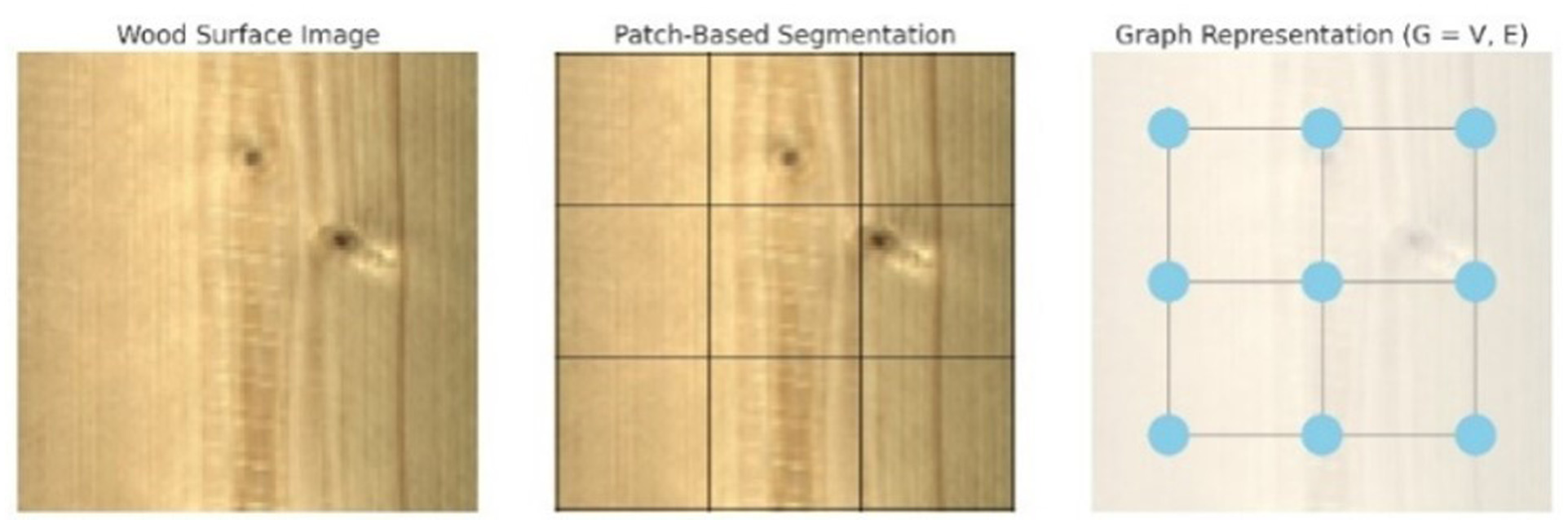
Graph representation (G = V, E).

Problem formulation

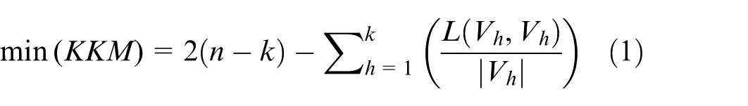
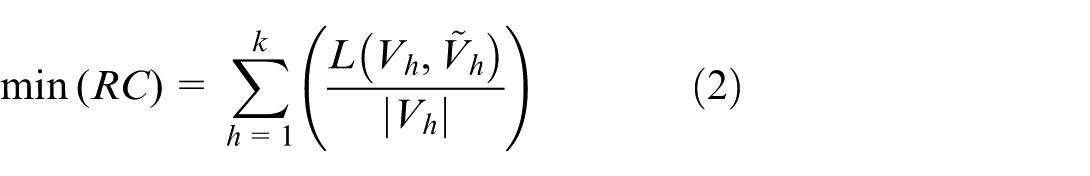
Authors formulate wood surface image segmentation as a multi-objective optimization problem by jointly minimizing the k-kernel mean (KKM) ⁶ (equation (1)) and the cutoff ratio (RC) ⁷ (equation (2)). These two objectives balance internal consistency within image segments and separation between distinct regions. The KKM metric captures the degree of compactness among nodes within the same cluster, encouraging strong intra-region similarity. In contrast, RC penalizes high connectivity between different clusters, promoting clearer boundary separation. Mathematically, we define the problem as follows.

$$min(\mathrm{KKM})=2(n-k)-\sum _{h=1}^k\left(\frac{L(V_h,V_h)}{\left|V_h\right|}\right)$$

(1)

$$min(\mathrm{RC})=\sum _{h=1}^k\left(\frac{L(V_h,{\tilde{V}}_h)}{\left|V_h\right|}\right)$$

(2)

With definition: $L(V_h,V_h)=\sum _{v_i,v_j\in V_h}{A}_{\mathrm{ij}}$ and $L(V_h,{\tilde{V}}_h)=\sum _{v_i\in V_h,v_j{V}_h}{A}_{\mathrm{ij}}$ .

Where $L(V_h,V_h)$ denotes the internal edge weight sum within the cluster V _h , and $L(V_h,{\tilde{V}}_h)$ refers to the total edge weight between clusters V _h and its complement. This formulation enables simultaneous optimization of both internal cohesion and external separation, critical for precise defect detection on wood surfaces.

A comprehensive visualization of the proposed graph-based wood image segmentation framework under a multi-objective optimization perspective. Subfigure illustrates the Pareto front depicting the trade-off between the two optimization objectives: k-kernel mean (KKM), which measures intra-cluster compactness, and cutoff ratio (RC), which quantifies inter-cluster separation. The curve demonstrates a typical conflict between objectives in multi-objective optimization, where improvement in one metric leads to degradation in the other. This behavior highlights the necessity of identifying a balanced clustering configuration that offers sufficient internal coherence while maintaining clear boundaries between image regions.

Subfigure provides a graph-based clustering representation of a wood surface image. The image is first partitioned into regular patches, each treated as a node in the graph. Each cluster corresponds to regions in the image with similar visual or textural properties. This diagram effectively demonstrates how the underlying graph structure, guided by the KKM and RC objectives, leads to meaningful segmentation of the wood surface, capturing both homogeneous textures and distinct pattern boundaries.

Multi-objective optimization

Multi-objective optimization problems in image feature processing often involve optimizing multiple objective functions simultaneously. The Pareto front plot illustrates the trade-off between two objectives (KKM and RCI), where each labeled point represents a non-dominated solution. Coordinates, reliability scores, and processing speed are annotated for each solution. Additionally, color intensity encodes the computational cost, providing a multi-dimensional view to support informed decision-making in multi-objective optimization.

In multi-objective optimization problems, achieving all objectives at the optimal level simultaneously is very difficult, or even impossible in many cases, because the objectives may conflict with each other. ⁸ In image processing, if you want to increase the accuracy of an image recognition model, you may have to accept longer processing times or consume more computational resources. Conversely, you may have to sacrifice some accuracy if you want to reduce processing time. This creates a conflict between different objectives. The concept of dominance is an important and commonly used concept in multi-objective optimization problems. Given two solution vectors $a=\{a_1,a_2,\dots ,a_n\}$ and $b=\{b_1,b_2,\dots ,b_n\};(a\ne b)$ . A vector solution dominates a vector solution b (denoted by a⪯b) if and only if $f_i\left(a\right)\le f_i\left(b\right);\forall i=1,2,\dots ,m$ and there exists at least one index i such that $f_i\left(a\right)<f_i\left(b\right)$ . Where f _i : is the i_th objective function, with i = 1,2,…,m representing the number of objectives in the multi-objective problem.

The Pareto front (PF) is the set of all Pareto optimal solutions in the objective space. The Pareto surface provides a set of optimal solutions to choose from, reflecting the diversity of options each solution offers. ⁹ This is similar to the decision problem in Arrow’s theory, ¹⁰ where trying to reconcile different preferences leads to conflict and the impossibility of reaching a single optimal solution.

In addition to Pareto-based selection, we employed two external metrics to evaluate the clustering quality: Silhouette Score (equation (3)) and Modularity (equation (4)). The Silhouette Score quantifies how well each patch is matched to its cluster versus others, capturing geometric cohesion. Modularity, on the other hand, measures the alignment of the clustering structure with the actual graph topology, penalizing random-like partitions. ¹¹ These metrics provide complementary insights and enhance the robustness of cluster validation.

$$\begin{array}{c}s\left(i\right)=\frac{b\left(i\right)-a\left(i\right)}{\max \{a\left(i\right),b\left(i\right)\}}\hfill \end{array}$$

(3)

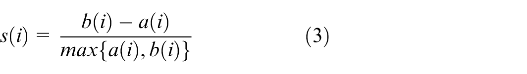
With a(i): average distance between point i and other points in the same cluster, and b(i): average between point i and the nearest points in other clusters.

$$\begin{array}{c}Q=\frac{1}{2m}\sum _{i,j}[A_{\mathrm{ij}}-\frac{k_i{k}_j}{2m}]\delta (c_i,c_j)\hfill \end{array}$$

(4)

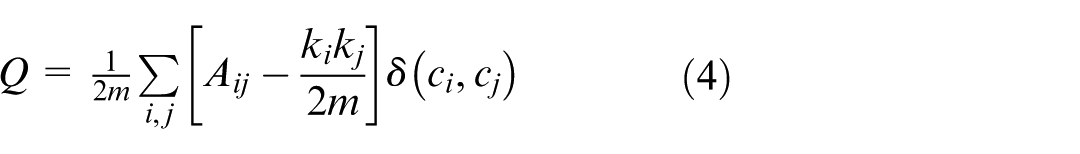
With A _ij : Edgeweight between node i and j.k _i : degree of node i, m: total number of edges and $\delta (c_i,c_j)=1$ : if i and j belong to the same cluster, otherwise 0.

Convolutional neural network (CNN)

The proposed Convolutional Neural Network (CNN) architecture ¹² for wood surface analysis begins with a 224 × 224 × 3 RGB image input. It sequentially applies convolutional layers with 3 × 3 kernels (64 and 128 feature maps), each followed by a Rectified Linear Unit (ReLU) activation and a 2 × 2 max pooling operation, effectively extracting local and hierarchical features. The resulting feature maps are flattened and passed to a fully connected layer with 128 units, followed by a Softmax classifier that outputs probabilities across defect classes. The mathematical formulation of the main CNN components is provided to clarify the feature extraction and classification process.

While the CNN module adopts a conventional architecture for low- and mid-level feature extraction, its role as the front-end of a hybrid framework substantially improves classification effectiveness. The Label Propagation Multi-objective Particle Swarm Optimization (LPMPSO) module optimizes multiple objectives such as precision, recall, and inter-class separation. Meanwhile, the Graph Attention Variational Autoencoder (GATVAE) captures global structural dependencies among extracted features by constructing graph-based representations from spatial and semantic similarities. ¹³ This combination allows the model to effectively integrate local texture information with contextual relationships across wood surface regions, resulting in more accurate, robust, and interpretable defect classification.

Label propagation multi-objective particle swarm optimization (LPMPSO)

In the proposed framework, the Particle Swarm Optimization (PSO) component operates within a multi-objective optimization setting, optimizing for clustering compactness (KKM), region separability (RC), and classification confidence. Each particle represents a candidate solution vector, updated iteratively according to equation (5), guided by both individual (personal best) and collective (global best) experiences.

$$\begin{array}{c}\{\begin{array}{c}{v}_{\mathrm{ij}}(t+1)=\omega .v_{\mathrm{ij}}\left(t\right)+c_1.r_1.(\mathrm{pbes}{t}_{\mathrm{ij}}-x_{\mathrm{ij}}\left(t\right))+c_2.r_2.(\mathrm{gbes}{t}_j-x_{\mathrm{ij}}\left(t\right))\hfill \\ \multicolumn{1}{c}{x_{\mathrm{ij}}(t+1)=x_{\mathrm{ij}}\left(t\right)+v_{\mathrm{ij}}(t+1)}\end{array}\hfill \end{array}$$

(5)

With ω: inertia weight controlling the impact of the previous velocity, $c_1,c_2$ Acceleration coefficients, which determine the influence of the personal and global best positions, $r_1,r_2$ : random values between 0 and 1 to add stochasticity, pbest _ij : personal best position of a particle i in dimension j and gbest _j : global best position in dimension j across all particles.

A repository is maintained to store Pareto-optimal solutions. Once the size exceeds a threshold, dominated or redundant entries are pruned, preserving only the non-dominated set (equation (6)).

$$\begin{array}{c}\mathrm{PF}=\{x\in \vartheta |x^{\prime }\in \vartheta \mathrm{such}\mathrm{that}F\left(x^{\prime }\right)<F\left(x\right)\}\hfill \end{array}$$

(6)

The selected solutions are utilized to construct an enhancement matrix E, which replaces the traditional adjacency matrix in the Graph Attention Variational Autoencoder (GATVAE) module. GATVAE encodes structural dependencies among features through attention-guided message passing and outputs refined latent representations. These embeddings are then fed back to LPMPSO to dynamically adjust objective preferences and particle behavior. This co-evolutionary feedback loop between LPMPSO and GATVAE enhances convergence stability, solution diversity, and classification robustness in wood surface defect analysis.

Graph attention neural network (GAT)

Graph Attention Network (GAT), proposed by Veličković et al., ¹⁴ extends traditional graph neural networks by introducing attention mechanisms to learn node-specific weights for neighboring connections. Each attention coefficient e _ij between node i and its neighbor j is computed. These coefficients are normalized using the softmax function. GAT also supports multi-head attention to improve learning stability and capture diverse relational patterns. The full GAT layer maps features from layer l to l + 1. Details of standard CNN/GAT formulations can be found in^12,14

In the proposed pipeline, wood surface images are processed through multiple stages. Initially, a Convolutional Neural Network (CNN) extracts localized visual patterns such as wood grain and surface defects. Next, Particle Swarm Optimization (PSO) is employed to optimize clustering and model parameters, facilitating enhanced intra-cluster compactness and inter-cluster separation. The Graph Attention Network (GAT) then models relationships among CNN-extracted features by treating them as nodes in a graph. GAT dynamically computes attention weights between node pairs, enabling the network to focus on semantically relevant features. This allows context-aware embedding construction that captures spatial dependencies across the wood surface. The resulting node embeddings are input to a Variational Autoencoder (VAE), which encodes them into a probabilistic latent space for regularization and improved generalization. Finally, a classification layer assigns each sample to a defect category or quality label. This combination of convolutional, evolutionary, and attention-based components offers a robust and interpretable solution for structured visual data analysis.

Graph attention neural network-variation autoencoder (GATVAE)

The Graph Autoencoder (GAE) ¹⁵ (Figure 4) aims to learn node embeddings h that can reconstruct the adjacency matrix A. Its loss is (equation (7)).

$$L_{\mathrm{GAE}}=E_{q(h|A)}.\left[\log p(A|h)\right]$$

(7)

With $q(h|A)$ : the probabilistic encoder and $p(A|h)$ : the probabilistic decoder.

The Variational GAE (VGAE) extends GAE by modeling each node’s embedding h _i as a Gaussian variable (equation (8)) and (equation (9)).

$$q(h|A)=\underset{i=1}{\overset{n}{\Pi }}q(h_i|A)$$

(8)

Where

$$q(h_i|A)=N\left(h_i|{\mu }_i,\mathrm{diag}({\sigma }_i^2)\right)$$

(9)

With μ _i : the mean vector and ${\sigma }_i^2$ : the variance for each dimension of the embedding.

The ELBO loss to minimize becomes (equation (10)).

$$L_R=E_{q(h|A)}.\left[\log p(A|h)\right]+\mathrm{KL}(q(h|A)\parallel p\left(h\right)$$

(10)

With $\mathrm{KL}(q(h|A)\parallel p(h)$ : The Kullback-Leibler divergence between the learned posterior $q(h|A)$ and the prior p(h).

This modification makes the VGAE model more flexible and effective in capturing both structural and feature information, enabling it to perform well on tasks such as link prediction and node clustering in attributed graphs.

Functional Analysis of the GAT-VAE Architecture: Input Graph Construction: Nodes represent visual patches (such as CNN features); edges define relations (spatial proximity or learned similarity. GAT Encoder: Two stacked GAT layers compute attention-weighted feature aggregation. The outputs are passed to two parallel MLPs (for mean and variance). Latent Sampling: Using reparameterization: $z_i={\mu }_i+{\sigma }_i\odot ϵ,ϵ~N(0,I)$ . Decoder (Inner Product): Reconstruct edge $A_{\mathrm{ij}}\approx \sigma (z_i^T{z}_j)$ , where σ is sigmoid. Application: Latent node embeddings are used for downstream tasks: classification, clustering, and defect detection.

Related works

Wood surface detection and classification based on deep learning

Deep learning techniques have significantly advanced the automation of wood surface defect detection and classification. CNN-based models have achieved high accuracy (>99%) in image-based classification tasks. Transfer learning applied on ResNet, DenseNet, and MobileNet architectures has further improved performance on large datasets.^16,17 Region-based detectors like Faster R-CNN have been used effectively for localization, achieving up to 99% accuracy, though with higher computational costs.^18,19 Single-stage detectors such as SSD and YOLO offer real-time processing capabilities, with YOLOv5m reaching 99.6% accuracy and 112 FPS.^20,21 Hybrid and segmentation approaches, including Deep LSD, NSST + CNN + ELM, and InceptionResNetV2, enhance detection accuracy for complex defect types and image modalities.^22,23 In parallel, PointNet++ and UNet have shown promise for 3D data and species classification tasks. ²⁴ Despite these advances, challenges remain, including the need for large annotated datasets, difficulty in detecting small or subtle defects, and dependency on high-end hardware. Several studies have proposed lightweight models or methods with reduced data requirements to address these limitations.^25,26 This body of work provides a solid foundation for developing robust, efficient, and scalable wood defect detection systems based on deep learning.

Wood surface detection and classification based on evolutionary algorithms

Recent studies have explored the integration of evolutionary algorithms with machine learning and deep learning models to improve wood surface defect detection. Genetic Algorithms (GA) have been widely used to optimize feature selection, ²⁷ segmentation parameters, ²⁸ and neural network architecture, ²⁹ leading to enhanced classification accuracy and reduced computational complexity. Chen et al. ³⁰ integrated Gabor filters and GA into Faster R-CNN, improving mAP from 78.98% to 94.57%. Ge et al. ³¹ and Xie et al. ³² enhanced YOLOv8s and RegNet, respectively, with attention and lightweight convolution modules, achieving over 96% accuracy and real-time performance (>160 FPS). Li et al. ³³ employed feature fusion and channel attention in YOLOX to handle multiple defect types with high accuracy (mAP 96.68%). In terms of system-level optimization, Wang et al. ³⁴ applied NSGA-II for solid wood layout optimization, while Xie et al. ³⁵ used differential evolution (DE) to tune an ensemble learning model for predicting surface roughness. These works demonstrate the effectiveness of evolutionary algorithms in enhancing detection accuracy, computational efficiency, and system adaptability in wood surface inspection applications.

Wood surface detection and classification based on graph neural network

Recent advances in surface defect detection have leveraged Auto-Encoder (AE)-based models and graph neural networks to improve detection and localization accuracy. For example, AEKD, ³⁶ CMA-AE, ³⁷ and MAAE ³⁸ integrate encoding-decoding architectures with knowledge distillation, memory modules, or attention mechanisms, achieving AUROC scores above 97% on standard datasets such as MVTec-AD. Graph-based models such as GAT and GCNN have shown promising results in hyperspectral image classification and surface defect recognition by capturing complex relationships between features. ³⁹ Bhatti et al. ⁴⁰ achieved up to 94.25% accuracy on the Indian Pines dataset using multi-feature fusion of 3D-CNN and improved GATs. Generative and attention-based anomaly detectors, including HaloAE, ⁴¹ LafitE, ⁴² and NDP-Net, ⁴³ have further improved anomaly localization through latent feature modeling and reference-based attention. These models have demonstrated performance gains of 2%–5% AUROC over previous state-of-the-art methods. In addition, hybrid methods such as GANs with attention fusion ⁴⁴ and texture-enhanced UAV classification ⁴⁵ have been explored for specialized applications, showing that anomaly detection frameworks can generalize across diverse domains. Collectively, these studies highlight the effectiveness of combining representation learning with attention and graph-based modeling for high-performance surface defect analysis, especially in unsupervised or weakly supervised industrial contexts.

Limitation of previous approaches on wood surface detection and classification

While numerous models have been proposed for industrial surface defect detection, most exhibit specific limitations when applied to the wood surface classification problem. Table 1 summarizes key prior approaches along with quantitative performance and technical drawbacks.

Table 1.

Quantitative comparison of prior methods for wood surface/defect classification.

Model	Accuracy (%)	Inference (FPS)	Strengths	Limitations
CNN 46	99.10	60	Simple to train, effective on clean patterns	Fails with noisy textures, low inter-class variance
YOLOv547	99.60	112	Fast detection, well-optimized	Poor at classifying micro-defects
MAAE 38	97.30	30	Excellent for anomaly detection	Sensitive to texture inconsistency and low resolution
HaloAE 41	97.80	18	Strong localization capability	Requires clean reference images, lacks domain flexibility
CheXNet 48	95.10	8	High accuracy in the medical domain	Overfits when applied to natural wood surfaces

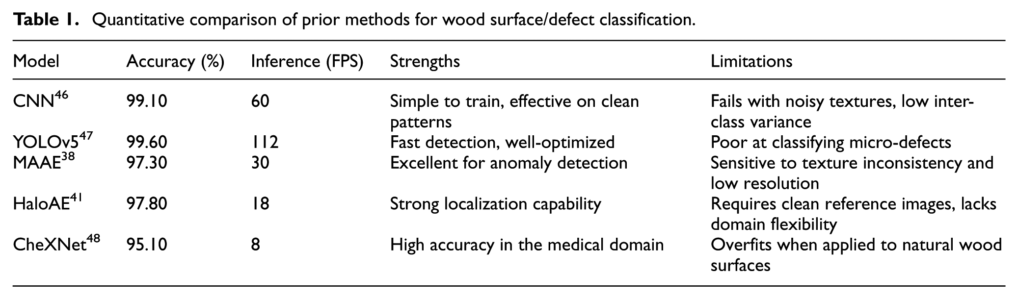
Texture Inconsistency: Unlike defects in metal or medical imaging, wood surfaces exhibit high intra-class texture variation (such as different grains, knots, sapwood rings), which can confuse CNNs and anomaly detectors like MAAE and HaloAE. These models often assume structural homogeneity, leading to high false positives when encountering natural wood patterns.

Lack of Contextual Modeling: Classical CNNs operate in a purely local pixel context. They do not model the topological relationships between regions of the image, which are crucial for correctly identifying elongated cracks or partial knots. Graph-based reasoning (GATVAE) is more effective in this case.

Overreliance on Reference Images: Methods like HaloAE require clean reference samples for anomaly detection, which are not feasible in the real-world wood processing pipeline, where every piece is unique. Thus, they lack generalizability.

No Feature Selection: Prior deep learning models often ignore irrelevant or redundant features, causing overfitting and reduced robustness. Feature selection techniques (PSO, genetic search) are essential to boost model interpretability and efficiency.

Related studies show that each group of methods has its own advantages and limitations. CNN models and one-stage detectors achieve high accuracy and speed, but often lack contextual modeling capabilities and are sensitive to the natural texture noise of wood. Evolutionary algorithm-based methods improve feature selection and parameter optimization but may encounter early convergence problems and do not fully exploit structural relationships. Meanwhile, autoencoder-based and GNN models perform strongly in representation learning and anomaly detection, but often depend on reference data or lack efficient feature selection mechanisms.

Proposed methodology

To enhance the detection and classification of wood surface features, recent approaches have focused on combining deep feature extraction, graph-based representation learning, and multi-objective optimization. The proposed LPMPSO-GATVAE-CNN framework integrates Convolutional Neural Networks (CNN) for 3D wood surface feature extraction, with a label-propagation-enhanced Particle Swarm Optimization (LPMPSO) module that optimizes feature selection through simultaneous minimization of KKM and Ratio Cut objectives. The enhanced features are then embedded via a Graph Attention Variational Autoencoder (GATVAE), which learns rich node representations. An iterative feedback loop between LPMPSO and GATVAE allows co-evolutionary refinement, improving both clustering performance and classification robustness (Figure 2). This tightly coupled design bridges representation learning and optimization, showing promise in complex industrial wood defect analysis tasks.

Figure 2.

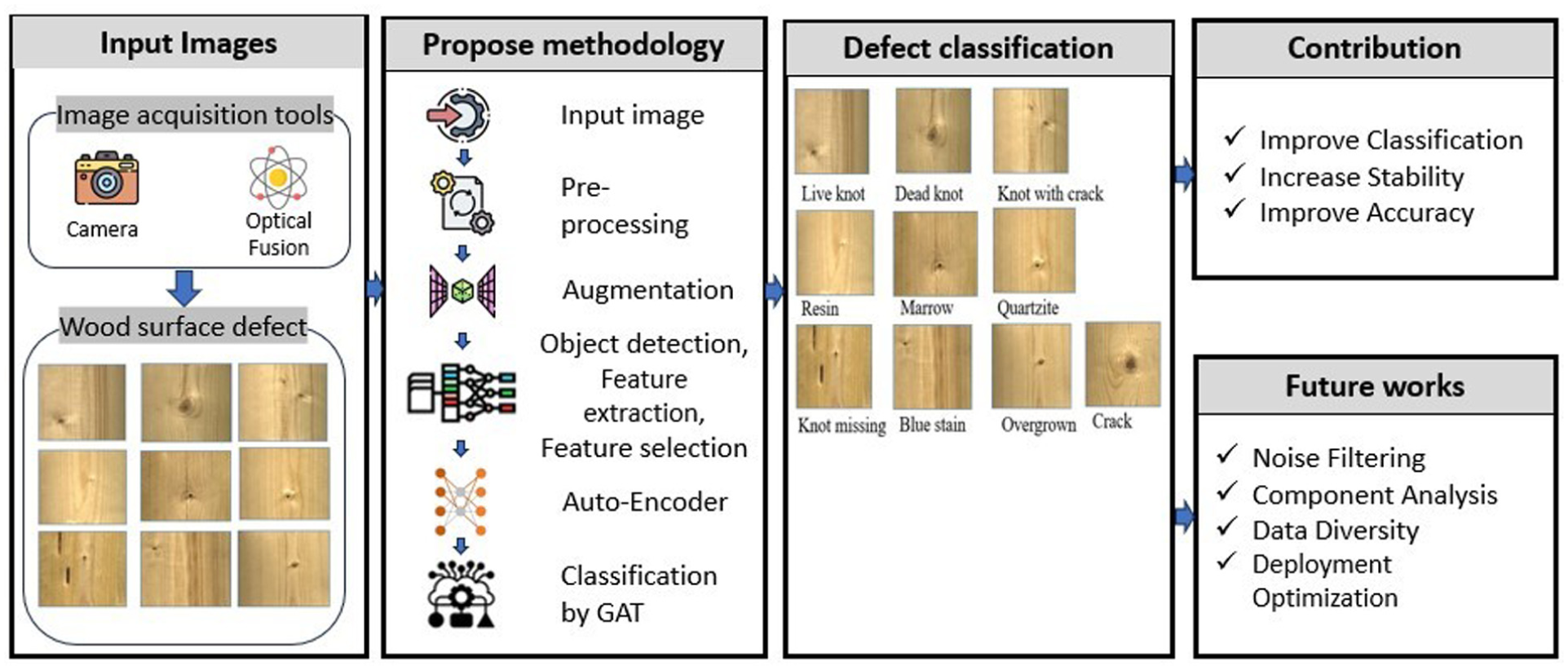
Proposed methodology.

Input wood surface image

In this study, input data were acquired through image acquisition tools, including cameras and Optical Fusion. Cameras were used to capture wood surfaces, while Optical Fusion allowed the combination of image data from multiple sensor sources, enhancing the quality and detail of the images. The captured objects were wood surface defects, which exhibited various types of defects such as cracks, knots, color spots, or surface deformation. These images served as important input data sources for the processing and classification of wood defects in the following steps.

Wood surface image processing

The important role of convolutional neural networks (CNNs) in computer vision, especially in small object recognition, is a major challenge because ROI pooling on the final feature map can lose important details. Advancements such as Feature Pyramid Networks (FPNs), ⁴⁹ Anchor-Free models, ⁵⁰ and Transformer-based models have partly solved this problem. A major limitation of VGG-16 is the reduction of small object features to a single pixel due to repeated strides and pooling, which leads to difficulty in object localization and recognition. To overcome the information loss problem in small object recognition, the CNN model proposed in this thesis extends the ROI pooling method by performing it on multiple feature maps instead of just using the final map. The Multi-level Feature Pooling technique projects ROIs onto multiple convolutional layers (Conv3, Conv4, Conv5) in VGG-16, ⁵¹ which helps maintain detailed information at multiple feature levels. The model also uses L2 regularization to ensure consistency when combining features from multiple layers, which helps improve accuracy and performance in recognizing small objects and objects of various sizes in real-world applications. Suppose (equation (11)) and (equation (12)). Describe the L2 normalization process for each pixel in the feature maps.

$$x=\frac{x}{{\Vert X\Vert }_2}$$

(11)

$${\Vert X\Vert }_2={\left(\sum _{i=1}^d\left|x_i^2\right|\right)}^{1/2}$$

(12)

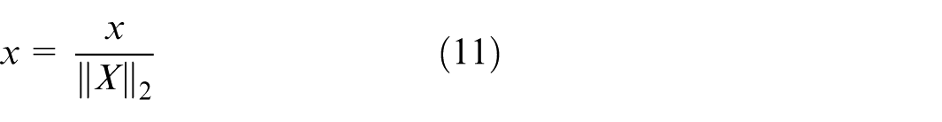
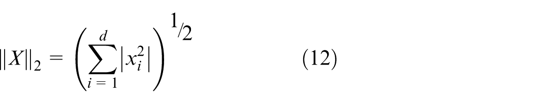
With x: original features, $\Vert X{\Vert }_2$ : normalized features, d: the sizes of the feature outputs from each convolutional layer.

During training, the feature normalization step corrects for scaling differences between channels of the feature map by using a scaling factor computed for each channel (equation (13)).

$$y_i={\lambda }_i\times X_i$$

(13)

With y _i : re-scaled feature value.

During the backpropagation process, the scaling factor λ _i can be calculated and adjusted to optimize the feature regularization process in the model. According to the backpropagation rule, equations (14)–(16) can be used to determine the value of λ _i , thereby improving the stability and convergence of the model.

$$\frac{\mathrm{dl}}{d\hat{x}}=\lambda \frac{\mathrm{dl}}{\mathrm{dy}}$$

(14)

$$\frac{\mathrm{dl}}{\mathrm{dx}}=\frac{\mathrm{dl}}{d\hat{x}}(\frac{I}{{\Vert X\Vert }_2}-\frac{\mathrm{xx}}{\Vert x{\Vert }_2^3})$$

(15)

$$\frac{\mathrm{dl}}{d{\lambda }_i}=\sum _{y_i}\frac{\mathrm{dl}}{y_i}\times x_i$$

(16)

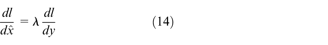
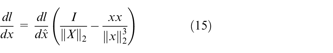
With $y\times [y_1,y_2,\dots ,y_d{]}^T$ .

Using 1 × 1 convolution along with fully connected layers is an effective method to reduce feature dimensionality, maintain detailed information, and enhance the model’s analytical ability in object localization and recognition tasks. Using a multi-task loss function in the object detection model is an important step to achieve high accuracy in both classification equation (17) and bounding box regression equation (18), ensuring that the model can effectively recognize and localize objects. The Cross-Entropy function represents the classification loss, which calculates the deviation between the actual label and the model’s prediction, equation (19).

$$L_{\mathrm{total}}=L_{\mathrm{classification}}+\alpha L_{\mathrm{boundingbox}}$$

(17)

$$L_{\mathrm{boundingbox}}=\mathrm{smoot}{h}_{L1}(\mathrm{bbo}{x}_{\mathrm{pred}}-\mathrm{bbo}{x}_{\mathrm{true}})$$

(18)

$$L_{\mathrm{classification}}=-\sum _{k=1}^K{y}_k\log \left({\hat{p}}_k\right)$$

(19)

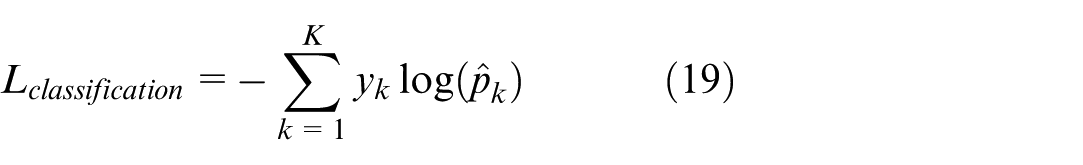
With L _{classification} : classification loss function, $L_{\mathrm{bounding}\mathrm{box}}$ : bounding box regression loss function, α: adjustment factor to balance between the two types of loss, bbox _pred : predicted bounding box coordinate, bbox _true : actual bounding box coordinate, K: total number of classes, y _k : actual label, ${\hat{p}}_k$ : predicted probability.

A one-hot encoding vector has K + 1 dimensions, providing a probability distribution representing the categories to which the sample may belong. This vector helps the model accurately classify the object while also determining when the object is absent in the ROI. This encoding is simple yet effective and is an important component of modern object detection models as $q=\{q_0,q_1,\dots ,q_k\}$ . In addition to the classification vector, the output of the model also contains a vector that specifies four adjusted coordinate values, denoted as $b=\{b_{\mathrm{cx}},b_{\mathrm{cy}},b_w,b_h\}$ . This vector defines the position and dimensions of the anticipated bounding box for the object within the ROI, aiding in precise object localization.

Label Propagation Based Multi-objective: In the wood surface label coding system for nodes in the network, the position of a particle p is represented by the label vector $X_p=[x_{p1},x_{p2},\dots ,x_{\mathrm{pn}}]$ with $x_{\mathrm{pi}}\in [1,n]$ : wood surface label of node and n: total number of nodes. In this model, the encoding process is performed and a wood surface label to each node. Nodes with the same label are grouped into the same wood surface. Based on this information, the decoding process helps to divide the original network into two wood surface clusters that represent the structure of the system. To initialize the positions of the particles in the model, the system uses the Label Propagation Algorithm (LPA), ⁵² in which each node is initially labeled with itself. This helps the nodes to automatically merge into wood surfaces optimally, accurately reflecting the surface structure in the network.

The weighted pooling-based label propagation strategy is designed to update the particle positions based on information from the local and global best particle positions, equations (20) and (21).

$$w_{\mathrm{ij}}\left(p\right)=\sum _{k\in N(i)}\mathrm{Ind}(x_{\mathrm{pj}},x_{\mathrm{pk}})$$

(20)

$$\mathrm{Ind}(a,b)=\{\begin{array}{c}1,a=b\hfill \\ \multicolumn{1}{c}{0,b\ne b}\end{array}$$

(21)

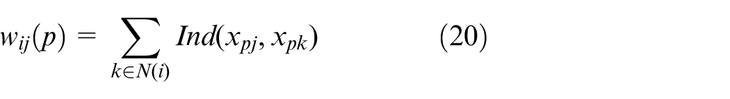
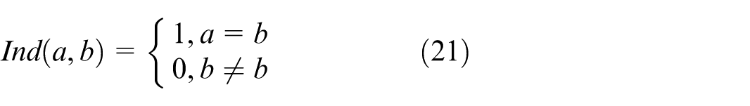
With $w_{\mathrm{ij}}\left(p\right)$ : reflects on neighbors.

When revising the position of particle p according to its local optimal position ( $\mathrm{lbes}{t}_p)$ or the global optimal position (gbest). Initially, adjust the weight connecting the node i to its adjacent node j (equation (22)).

$${\hat{w}}_{\mathrm{ij}}=w_{\mathrm{ij}}\left(p\right)+w_{\mathrm{ij}}\left(\mathrm{lbes}{t}_i\right)+w_{\mathrm{ij}}\left(\mathrm{gbest}\right)$$

(22)

With ${\hat{w}}_{\mathrm{ij}}$ : the sum of the weight.

The procedure for revising the wood surface label of the node i relies on the label of the neighboring node with the greatest weight, aiming to optimize the wood surface allocation in the network, equations (23) and (24).

$$s=\mathrm{argma}{x}_i\times {\hat{w}}_{\mathrm{ij}},j\in N\left(i\right)$$

(23)

$$x_{\mathrm{pi}}=x_{\mathrm{ps}}$$

(24)

With s: index of the neighbor with the highest weight, ${\hat{w}}_{\mathrm{ij}}$ : weight.

The process of optimizing the wood surface segmentation in the network by updating the labels based on the neighboring nodes and using multi-objective optimization with two functions, KKM and RC. The Pareto front is applied to achieve a reasonable wood surface structure, while the modularity index is used to evaluate the clarity of this structure. A high modularity shows that the wood surfaces are reasonably divided. In the multi-objective PSO model, modularity is used as a criterion to update the local best and global best, which helps to orient the PSO kernel to the optimal surface structure, more accurately reflecting the relationship between nodes in the network equation (25).

$$Q=\frac{1}{2m}\sum _{v\in V}\sum _{w\in V}(A_{\mathrm{vw}}-\frac{k_v{k}_w}{2m})\delta (c_v,c_w)$$

(25)

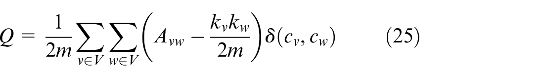
With m: number of edges, $k_v{k}_w$ : degree of a node.

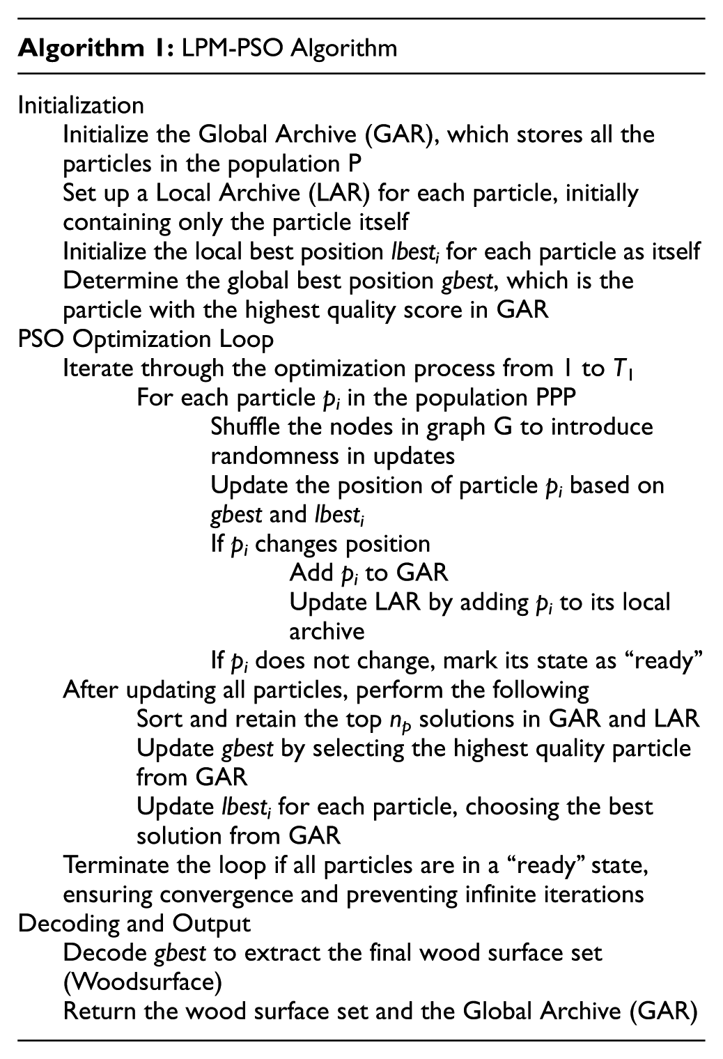
The LPM-PSO (Label Propagation-based Multi-objective Particle Swarm Optimization) algorithm number 1 is designed to optimize the partitioning of wood surfaces in a graph G(V, E, A). It utilizes PSO to find an optimal wood surface structure by iteratively updating the particle positions based on local and global best states.

Algorithm 1: LPM-PSO Algorithm
Initialization
	Initialize the Global Archive (GAR), which stores all the particles in the population P
	Set up a Local Archive (LAR) for each particle, initially containing only the particle itself
	Initialize the local best position lbest i for each particle as itself
	Determine the global best position gbest, which is the particle with the highest quality score in GAR
PSO Optimization Loop
	Iterate through the optimization process from 1 to T1
		For each particle p i in the population PPP
			Shuffle the nodes in graph G to introduce randomness in updates
			Update the position of particle p i based on gbest and lbest i
			If p i changes position
				Add p i to GAR
				Update LAR by adding p i to its local archive
			If p i does not change, mark its state as “ready”
	After updating all particles, perform the following
		Sort and retain the top n p solutions in GAR and LAR
		Update gbest by selecting the highest quality particle from GAR
		Update lbest i for each particle, choosing the best solution from GAR
	Terminate the loop if all particles are in a “ready” state, ensuring convergence and preventing infinite iterations
Decoding and Output
	Decode gbest to extract the final wood surface set (Woodsurface)
	Return the wood surface set and the Global Archive (GAR)

Built Enhanced Matrix: Using the reinforcement matrix and CIM effectively embeds the LPMPSO wood surface into GATVAE, thereby improving the model’s ability to represent and learn the network structure while reducing overfitting. The augmentation matrix A _eh , constructed from the adjacency matrix A and the second-order CIM matrix M, is a powerful tool to enhance the connections within the same wood surface, helping the model to better learn the wood surface structure in the network. The use of A _eh allows the model to maintain high coherence within the wood surface, thereby optimizing the learning and detection performance of wood surfaces in complex network analysis applications (equation (26)).

$$A_{\mathrm{eh}}=A+M$$

(26)

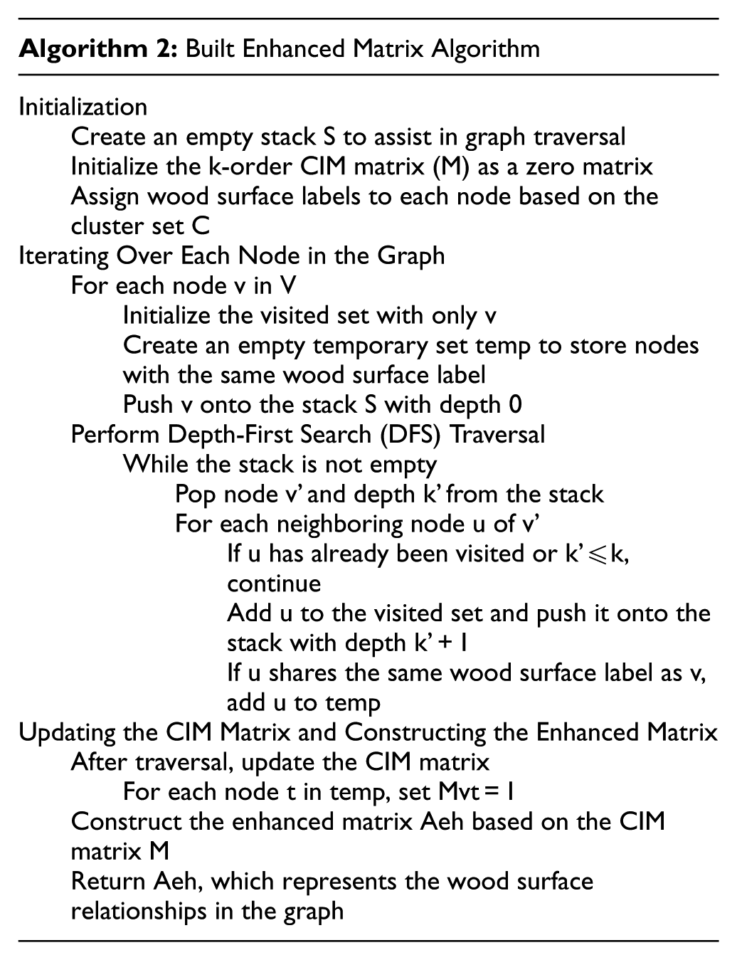
The Built Enhanced Matrix algorithm number 2 is designed to construct the enhanced matrix A _eh based on the graph structure and wood surface clusters. It leverages k-order CIM (Common Influence Matrix) to determine relationships between nodes in graph G(V, E, A) and optimizes wood surface structure analysis.

Algorithm 2: Built Enhanced Matrix Algorithm
Initialization
	Create an empty stack S to assist in graph traversal
	Initialize the k-order CIM matrix (M) as a zero matrix
	Assign wood surface labels to each node based on the cluster set C
Iterating Over Each Node in the Graph
	For each node v in V
		Initialize the visited set with only v
		Create an empty temporary set temp to store nodes with the same wood surface label
		Push v onto the stack S with depth 0
	Perform Depth-First Search (DFS) Traversal
		While the stack is not empty
			Pop node v’ and depth k’ from the stack
			For each neighboring node u of v’
				If u has already been visited or k’≤k, continue
				Add u to the visited set and push it onto the stack with depth k’+1
				If u shares the same wood surface label as v, add u to temp
Updating the CIM Matrix and Constructing the Enhanced Matrix
	After traversal, update the CIM matrix
		For each node t in temp, set Mvt = 1
	Construct the enhanced matrix Aeh based on the CIM matrix M
	Return Aeh, which represents the wood surface relationships in the graph

Wood surface image classification

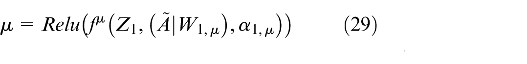
Graph Attention Variational Autoencoder: In this thesis, a novel variation of VGAE, combined with GAT, referred to as GATVAE, is designed to learn embedding vectors from the enhancement matrix A _eh . After these embedding vectors are learned, they are partitioned into clusters using the Fuzzy C-means (FCM) algorithm (equations (27)–(31)). GATVAE, with a VGAE encoder consisting of two GAL layers, leverages the enhancement matrix to learn embedding vectors that reflect the wood surface structure. These embedding vectors are then clustered using FCM, allowing efficient updating of kernels in LPMPSO. This approach improves the accuracy of wood surface structure detection and optimization, especially in complex networks.

$$\overline{A}={\hat{D}}^{\frac{1}{2}}(A_{\mathrm{eh}}+I){\hat{D}}^{\frac{1}{2}}$$

(27)

$$Z_1=\mathrm{Relu}\left(f(Z_0,(\tilde{A}|W_0),{\alpha }_0)\right)$$

(28)

$$\mu =\mathrm{Relu}\left(f^{\mu }(Z_1,(\tilde{A}|W_{1,\mu }),{\alpha }_{1,\mu })\right)$$

(29)

$${\sigma }^2=\mathrm{Relu}\left(f^{\sigma }(Z_1,(\tilde{A}|W_{1,\sigma }),{\alpha }_{1,\sigma })\right)$$

(30)

$$Z_2=q\left((Z|N)(\mu ,{\sigma }^2)\right)$$

(31)

In this model, the $A_{\mathrm{eh}}+I$ matrix, an enhanced diagonal matrix, is used as input to learning node embeddings in feature-free networks. This encoding and decoding process, through GATVAE with graph attention layers (GAL), enables the model to learn complex node embeddings from the enhanced A _eh matrix. This approach helps the model maintain the wood surface structure during embedding learning and allows for accurate reconstruction of the original adjacency matrix, ensuring effective network structure modeling (equation (32)).

$$\overline{A}=\sigma \left(Z_2{Z}_2^T\right)$$

(32)

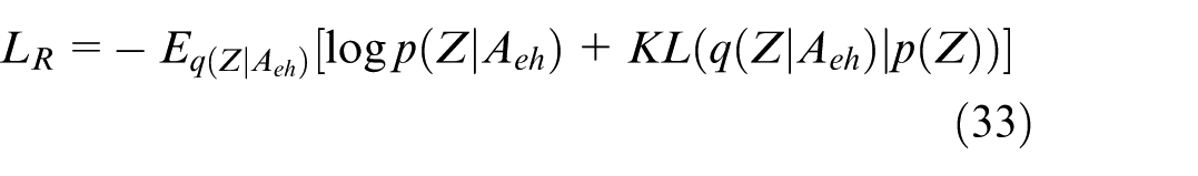
In this improved VGAE model, the A _eh matrix (enhanced matrix) is also incorporated into the VGAE loss function to aid the embedding learning process. Adding A _eh to the loss function helps the model maintain important information from the wood surface structure, optimizes the learning of the embedding representation, and improves the accuracy of the network reconstruction (equation (33)).

$$L_R=-E_{q(Z|A_{\mathrm{eh}})}[\log p(Z|A_{\mathrm{eh}})+\mathrm{KL}(q(Z|A_{\mathrm{eh}})|p\left(Z\right))]$$

(33)

Hybrid optimization model: The CNN-LPMPSO-GATVAE algorithm number 3 is a hybrid optimization model combining Particle Swarm Optimization (PSO), Graph Attention Networks (GAT), Variational Autoencoders (VAE), and fuzzy clustering techniques to optimize the partitioning of wood surfaces in a graph G(V, E, A). The goal is to generate a Pareto front (PF) that reflects the best possible solution for wood surface partitioning and structure.

Algorithm 3: CNN-LPMPSO-GATVAE
Initialization
	Generate a swarm P with n p particles, initializing the position of each particle
	Initialize the Global Archive (GAR) as an empty set θ
Wood Surface Partitioning via LPMPSO
	Run the LPMPSO algorithm for the initial particle swarm to partition the wood surface and update the Global Archive (GAR)
	Return the wood surface labels and the updated GAR
Multi-objective Optimization Loop
	For each iteration i from 1 to T2
		Generate Enhanced Matrix: Compute the Enhanced Matrix Aeh based on the graph G, the CIM order k, and the current wood surface labels
		Apply GATVAE: Use the Graph Attention Variational Autoencoder (GATVAE) to process Aeh and obtain the latent representations
		Determine the bounds of the wood surface number
			Compute the lower bound c low and upper bound c high of the number of wood surfaces in the solutions within GAR
		Calculate step size
			Set the step size as step $=\frac{c_{\mathrm{high}}-c_{\mathrm{low}}}{n_p}$
		Fuzzy Clustering Update
			For each particle p in P, use fuzzy c-means clustering to assign it to a wood surface cluster Cp based on the current solution set Z.
			Update the particle position according to Cp
		Update wood surface partitioning
			Run the LPMPSO algorithm again to update the wood surface labels and the Global Archive (GAR)
		Termination
			Repeat steps until the specified number of iterations T2 is completed
		Return Pareto Front
			Return the Pareto front PF from the Global Archive (GAR), which contains the optimal solutions for wood surface partitioning

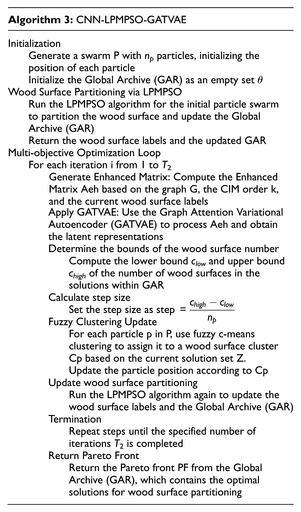
Meaning of each step in CNN-LPMPSO-GATVAE: Step 1 (LPMPSO): Provide a preliminary foundation to determine the wood surface structure and initialize clusters and particles with initial information. Step 2 (GATVAE with enhanced matrix): Optimize the embedding vectors with enhanced wood surface relationships, ensuring that nodes in the same wood surface have stronger connections. Step 3 (Limit the number of wood surface clusters): Set an optimal range for the number of wood surfaces, ensuring that the clustering achieves a reasonable structure that is not too fragmented or aggregated. Thanks to these steps, CNN-LPMPSO_GATVAE achieves a more accurate wood surface structure and maintains the consistency of clusters in the network, which helps to optimize the accuracy of the wood surface structure analysis model. The optimization procedure in CNN-LPMPSO_GATVAE, with T₂ iterations uses the Pareto front, and the candidate values from the wood surface count to optimize fuzzy c-means clustering, which significantly improves the model accuracy. Employing the evaluation metric to choose the optimal solution from the Pareto front guarantees that the wood surface structure of the network is optimized and accurately reflects the complex network data. In the closed-loop feedback mechanism, the latent representation Z₂ learned by the GATVAE is used to update PSO particles through the fuzzy clustering result C _p . Specifically, each particle is reassigned to surface clusters based on distances in the Z₂ latent space, which directly modifies the particle position vector x _ij to reflect the newly learned embedding structure. The particle velocity v _ij is subsequently influenced through the standard PSO update rule in the next iteration, ensuring co-evolution between PSO optimization and GATVAE representation learning.

Complexity Analysis: The overall time complexity of LPMPSO_GAVAE represents the integration of the optimization, embedding, and clustering phases, ensuring accurate embedding and optimizing the wood surface structure in the network, which is divided into three main components.

• Part 1: The time complexity of LPMPSO is O((np2 + m·np)·T1) ). The main factors affecting this complexity include the size of the swarm np, the number of edges m, and the number of iterations T₁. This analysis helps to clarify the factors that govern the computational time in the optimization process of LPMPSO in the LPMPSO_GATVAE framework.

• Part 2: The time complexity of GATVAE depends on the number of nodes and edges in the network, the number of input features, the dimensionality of the output vector, the number of attention heads in GAT, the highest iteration count, and the cluster quantity in Fuzzy C-means. This analysis helps to clarify the factors that govern the computation time in GATVAE when integrated into the LPMPSO_GATVAE framework.

The above graph shows the loss during the training process of the Autoencoder model, with the horizontal axis being the number of epochs and the vertical axis being the MSE Loss (Mean Squared Error) value (Figure 3). Initially, the loss value is very high (about 0.16), but it decreases rapidly after the first few epochs, showing that the model learns the data structure effectively. After about 20 epochs, the loss curve is almost stable around a very low level, fluctuates slightly, and almost approaches 0 when reaching about 100 epochs. This shows that the model has converged well, there is no obvious overfitting phenomenon, and it can reproduce the input data with very small errors. In other words, the autoencoder has learned the hidden features of the data effectively, ensuring high performance for compression or anomaly detection tasks in the later stages.

Figure 3.

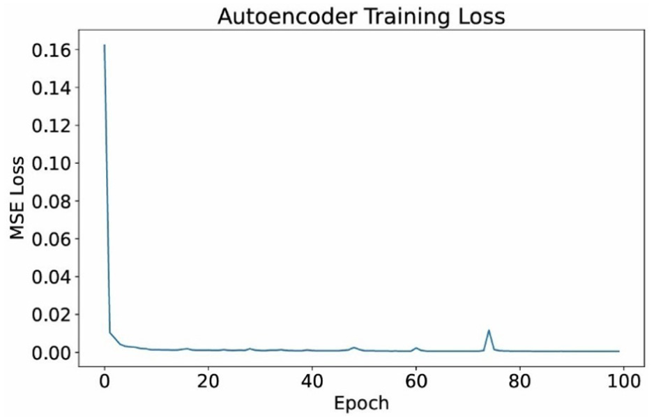
Autoencoder training loss.

The above graph is a Histogram of Reconstruction Errors of the Autoencoder model on the test set (Figure 4). The horizontal axis represents the reconstruction error (MSE), while the vertical axis represents the density of the data samples. Two different colors represent two groups: Normal and Defect. Observing the graph, it can be seen that most of the samples have very small errors, concentrated around a value close to 0, especially the “Normal” group. However, the “Defect” group tends to have a slightly higher reconstruction error, indicating that the model has difficulty reproducing data with defects. This shows that the Autoencoder model has learned the features of normal data well, so when encountering abnormal samples, the error increases - this is a sign that the model can be used effectively in detecting defects or anomalies in wood data.

• Part 3: The overall time complexity of LPMPSO_GAVAE is $0(T_2·(n_p^2+m·n_p))·T_1+(\mathrm{nF}+m)·R·L+n·R·T_k+n·d·k$ . By optimizing the number of iterations T₁ and T₂, the algorithm can achieve higher efficiency and handle large networks, ensuring accurate wood surface structure and effective clustering.

Figure 4.

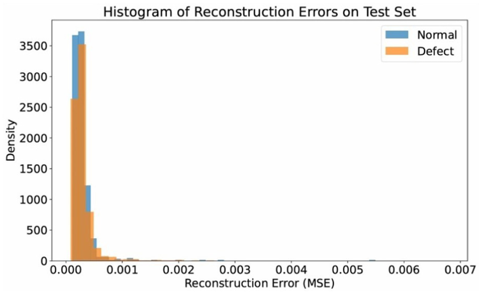
Histogram on reconstruction.

Result and experience

Datasets

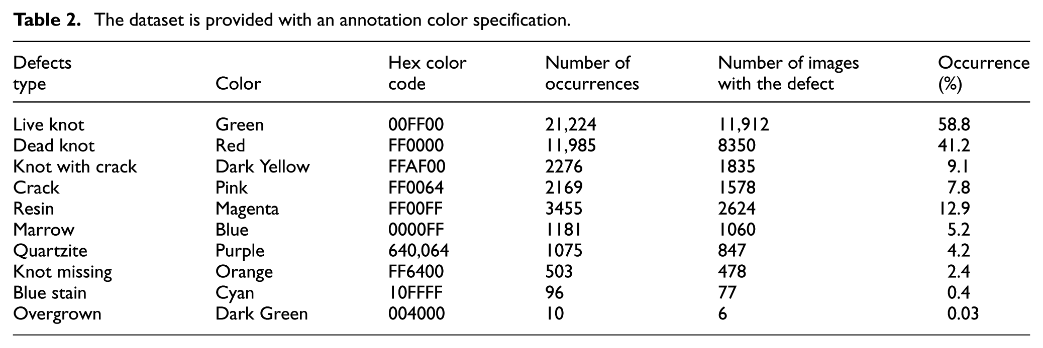
The dataset used in this thesis was acquired by Pavel Kodytek and his team at the VSB-TU Ostrava (2022). ⁵³ For the image acquisition of moving wood pieces was used line scan camera connected to the frame grabber by Camera Link interface. Silicon Software’s micro-Display X framegraber was used to transfer data from the camera into PCTo filter meaningless data, an offline histogram-based algorithm was created, reducing the dataset to 20,275 images and performing image cropping to reduce file size and computation time. Labeling was performed manually by trained personnel. The experimental data details are presented in Table 2.

Table 2.

The dataset is provided with an annotation color specification.

Defects type	Color	Hex color code	Number of occurrences	Number of images with the defect	Occurrence (%)
Live knot	Green	00FF00	21,224	11,912	58.8
Dead knot	Red	FF0000	11,985	8350	41.2
Knot with crack	Dark Yellow	FFAF00	2276	1835	9.1
Crack	Pink	FF0064	2169	1578	7.8
Resin	Magenta	FF00FF	3455	2624	12.9
Marrow	Blue	0000FF	1181	1060	5.2
Quartzite	Purple	640,064	1075	847	4.2
Knot missing	Orange	FF6400	503	478	2.4
Blue stain	Cyan	10FFFF	96	77	0.4
Overgrown	Dark Green	004000	10	6	0.03

Experimental setup

Fairness in comparison is ensured by using the same dataset, the same training/testing split strategy, and the same evaluation metrics for all control and proposed models. The methods being compared are retrained in the same hardware environment, with equivalent epochs and stop conditions, and hyperparameters are set according to the original recommendations or fairly fine-tuned through preliminary testing. As a result, performance differences accurately reflect method superiority rather than training configuration.

The parameters and hyperparameters of the model are set to optimize performance and achieve high accuracy during training and testing. The reasonable configuration helps reduce computation time, avoid overfitting and underfitting, and support rapid convergence. The system uses an Intel Core i7-7600U processor, 32 GB of RAM, and an NVIDIA GeForce RTX3060 GPU with 12 GB of graphics memory to accelerate the training process. The operating system is Ubuntu 20.04, Python 3.7, and CUDA 11.3, along with the TensorFlow library version 2.9. During training, the batch size is set to 128, the learning rate is 0.01, and the input image is resized to 640 × 640. The model is trained for 1000 epochs with the Adam optimization algorithm, which achieves high performance and improves the accuracy of the model.

Wood surface image processing

To measure segmentation performance, three main metrics are used: (1) Accuracy is the ratio of the number of correctly segmented pixels to the total number of pixels (equation (34)). (2) Sensitivity (or Recall) is the ratio of true positive pixels to the total number of true positive pixels (equation (35)). (3) Dice Similarity Coefficient (DSC; equation (36)).

$$\mathrm{PPV}=\frac{\mathrm{TP}}{\mathrm{TP}+\mathrm{FP}}$$

(34)

$$\mathrm{SEN}=\frac{\mathrm{TP}}{\mathrm{TP}+\mathrm{FN}}$$

(35)

$$\mathrm{DSC}=\frac{2·\mathrm{TP}}{2·\mathrm{TP}+\mathrm{FP}+\mathrm{FN}}$$

(36)

With segmentation’s false negative (FP), true negative (TN), false positive (FP), and true positive (TP) values.

With this requirement, to complete the evaluation of the used wood surface dataset segmentation strategy, specific steps have to be done: Prepare Data for Visual Evaluation with the first column, including input images. The second column is the pre-processed image (grayscale image). The third column is the processed segmentation image (shown in Table 3 to calculate the metrics; accuracy, sensitivity, and DSC similarity coefficient), a ground truth image of the actual segmentation region is needed. The ground truth is a labeled image of the same size as the input image, in which the pixels are correctly labeled for each region of interest. Once the ground truth image is obtained, the performance metrics for each image in the wood surface dataset can be calculated.

Table 3.

Segmented images of the wood surface image dataset.

Class	Original image	CLAHE	Canny edge	HSV	Final image
Live knot
Dead knot
Knot with crack
Crack
Resin
Marrow
Quartzity
Knot missing
Blue stain
Overgrown

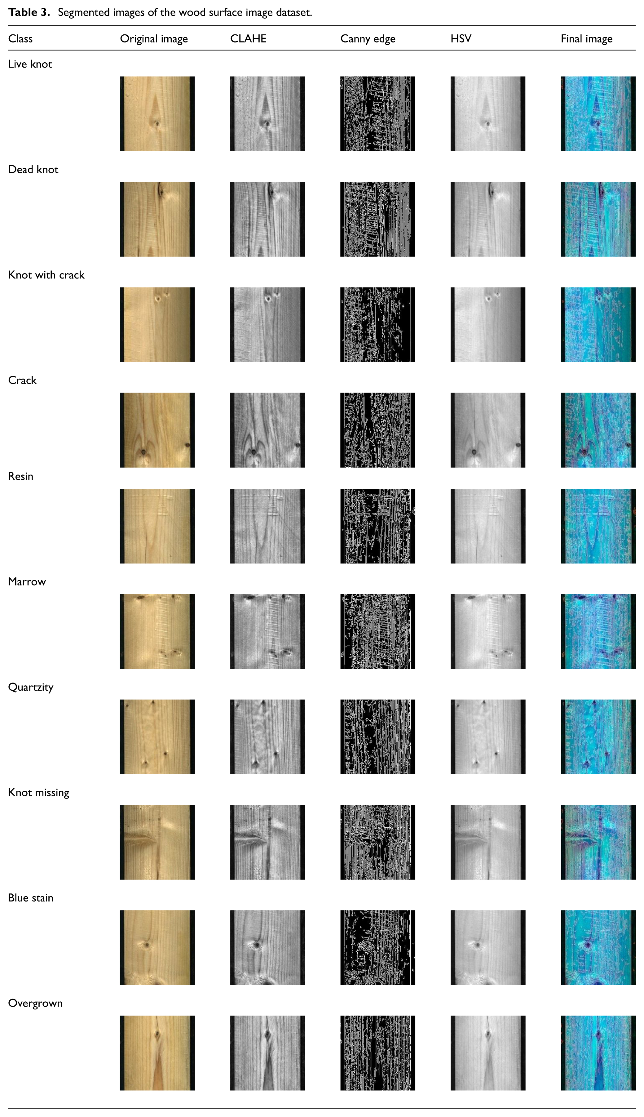
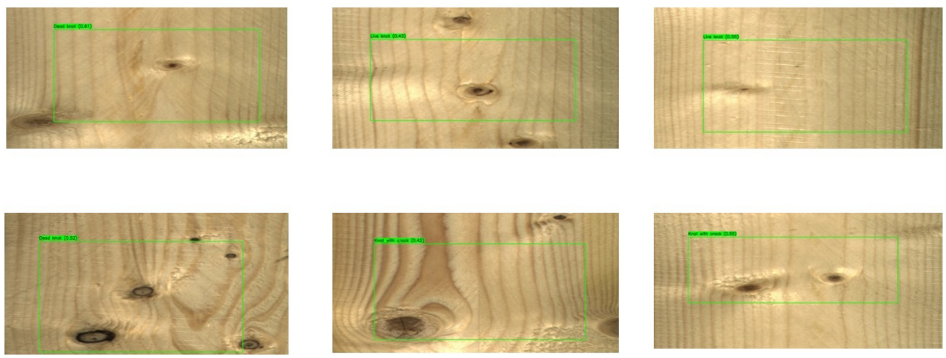
The wood surface segmentation process includes the following main steps: (1) Background processing to remove unnecessary details and highlight areas of interest; (2) Wood knot segmentation using algorithms such as Otsu thresholding or edge filtering; (3) Labeling and grouping wood knot regions based on shape or color; (4) Processing adjacent regions using edge extraction or distance classification techniques to avoid overlap and accurately identify. Figure 5 shows the image above, which illustrates the results of detecting and classifying defects on the wood surface using a deep learning model. Each image shows a wood board with defect areas delineated and labeled as Live knot, Dead knot, Knot with crack, Resin, or Marrow. This recognition shows that the model is capable of distinguishing different types of defects with a fairly high location accuracy. The system not only identifies the defect areas but also classifies them according to physical characteristics, helping to automate the wood quality inspection process. Thanks to this, the production process can minimize manual errors, increase efficiency, and ensure product consistency.

Figure 5.

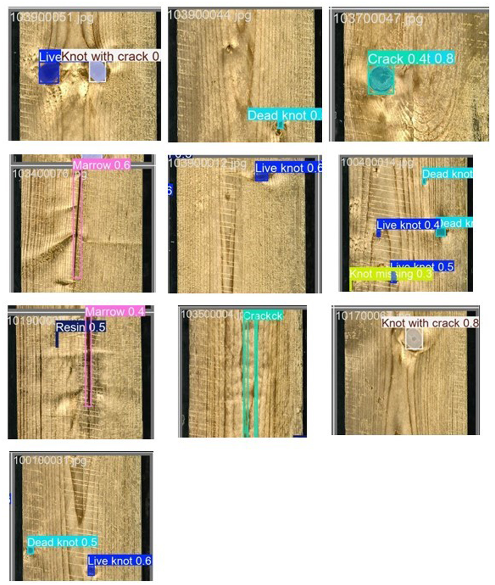
Wood surface defect detection analysis.

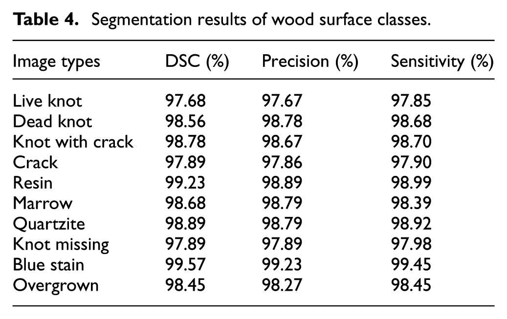
To generate the performance metrics (DSC, precision, and sensitivity) for each layer in the wood surface dataset, the mentioned values have to be calculated based on the segmentation image and the ground truth image for each layer (shown in Table 4) After calculating the metrics for each sample, the standard deviation for each metric (DSC and precision) can be calculated to evaluate the stability of the method.

Table 4.

Segmentation results of wood surface classes.

Image types	DSC (%)	Precision (%)	Sensitivity (%)
Live knot	97.68	97.67	97.85
Dead knot	98.56	98.78	98.68
Knot with crack	98.78	98.67	98.70
Crack	97.89	97.86	97.90
Resin	99.23	98.89	98.99
Marrow	98.68	98.79	98.39
Quartzite	98.89	98.79	98.92
Knot missing	97.89	97.89	97.98
Blue stain	99.57	99.23	99.45
Overgrown	98.45	98.27	98.45

Wood surface image classification

Performance metrics for classification: To evaluate the performance of a classification system, common performance metrics such as Overall Accuracy (equation (37)), Precision (equation (38)) which indicates the proportion of true positive predictions that are correct, Sensitivity (equation (39)) which indicates the model’s ability to detect positive cases correctly, Specificity (equation (40)) which measures the model’s ability to detect negative cases correctly, F1 Score (equation (41)) which is a harmonic mean of sensitivity and precision, useful when a trade-off between accuracy and sensitivity is required.

$$\mathrm{Accuracy}=\frac{\mathrm{TrP}+\mathrm{TrN}}{\mathrm{TrP}+\mathrm{TrN}+\mathrm{FsP}+\mathrm{FsN}}$$

(37)

$$\mathrm{Precision}=\frac{\mathrm{TrP}}{\mathrm{TrP}+\mathrm{FsP}}$$

(38)

$$\mathrm{Sensitivity}(\mathrm{recall})=\frac{\mathrm{TrP}}{\mathrm{TrP}+\mathrm{FsN}}$$

(39)

$$\mathrm{Specificity}=\frac{\mathrm{TrN}}{\mathrm{TrN}+\mathrm{FsP}}$$

(40)

$$F1-\mathrm{Score}=\frac{2·\mathrm{Precision}·\mathrm{recall}}{\mathrm{Precision}+\mathrm{recall}}$$

(41)

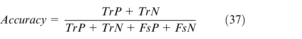
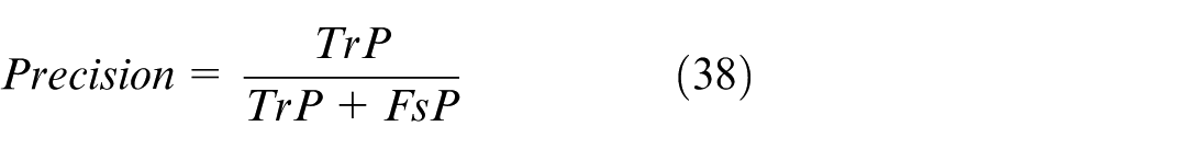
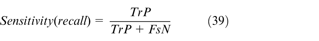
False Negative (FsN): Is the number of target wood surface types missed or incorrectly identified by the system? These are the target wood surface samples that the model does not detect or incorrectly detects. True Positive (TrP) is the number of target wood surface types that are correctly identified. These are the cases where the model correctly classifies the required wood surfaces. True Negative (TrN) is the number of regions that are detected and identified as not being the target wood surface. These objects are not part of the target wood surface and have been correctly classified by the model. False Positive (FsP) is the number of regions mistakenly classified as the target wood surface, while not the required wood surface? This reflects errors in misidentifying unrelated regions as wood surfaces. Based on these definitions, you can apply the formulas for calculating Accuracy, Sensitivity, Specificity, Precision, and F1 Score as presented in the previous section to evaluate the performance of the wood surface classification system.

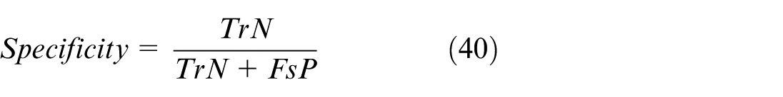
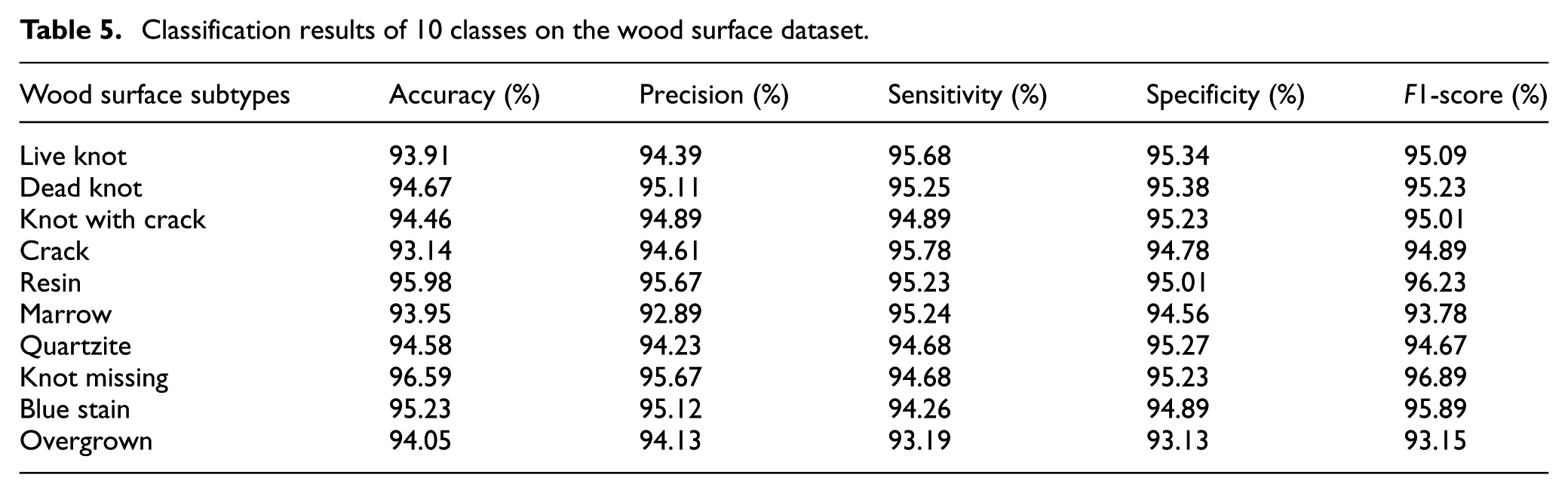
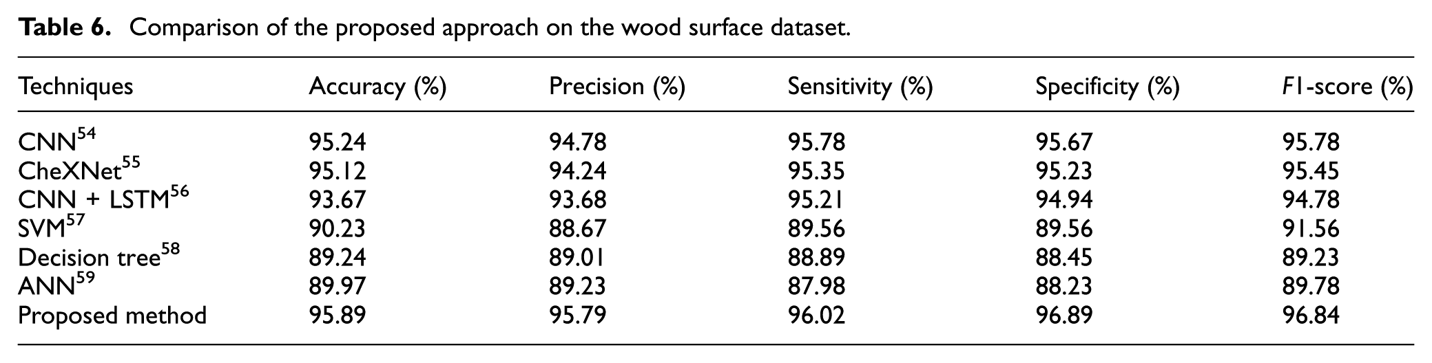
Classification results on wood surface datasets: The results of wood surface image classification from this thesis show that the proposed method has the best performance compared to other techniques. The analysis shows that the “Knot missing” and “Resin” images have the best performance, while the “Overgrown” image has the worst result. This method outperforms classical methods such as SVM and Decision Tree, thanks to the improvement in architecture and machine learning techniques, which helps to improve sensitivity and reduce the number of false detections, as shown in Figure 6 and Table 5, and with the highest Accuracy, Precision, Sensitivity, Specificity, and F1-score. Specifically, the accuracy is 95.89%, the Precision is 95.79%, the Sensitivity is 96.02%, and the Specificity is 96.89%, showing the ability to classify accurately and reduce false detections as shown in Figure 7 and Table 6. This proves the feasibility of the method in automatic wood surface quality monitoring systems (Figure 8).

Figure 6.

Graphical representation of 10 defect class classifications on the wood surface dataset.

Table 5.

Classification results of 10 classes on the wood surface dataset.

Wood surface subtypes	Accuracy (%)	Precision (%)	Sensitivity (%)	Specificity (%)	F1-score (%)
Live knot	93.91	94.39	95.68	95.34	95.09
Dead knot	94.67	95.11	95.25	95.38	95.23
Knot with crack	94.46	94.89	94.89	95.23	95.01
Crack	93.14	94.61	95.78	94.78	94.89
Resin	95.98	95.67	95.23	95.01	96.23
Marrow	93.95	92.89	95.24	94.56	93.78
Quartzite	94.58	94.23	94.68	95.27	94.67
Knot missing	96.59	95.67	94.68	95.23	96.89
Blue stain	95.23	95.12	94.26	94.89	95.89
Overgrown	94.05	94.13	93.19	93.13	93.15

Figure 7.

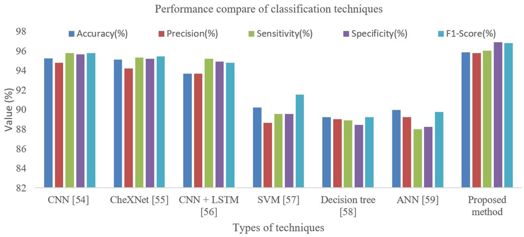
Comparison of classification results on the wood surface dataset.

Table 6.

Comparison of the proposed approach on the wood surface dataset.

Techniques	Accuracy (%)	Precision (%)	Sensitivity (%)	Specificity (%)	F1-score (%)
CNN 54	95.24	94.78	95.78	95.67	95.78
CheXNet 55	95.12	94.24	95.35	95.23	95.45
CNN + LSTM 56	93.67	93.68	95.21	94.94	94.78
SVM 57	90.23	88.67	89.56	89.56	91.56
Decision tree 58	89.24	89.01	88.89	88.45	89.23
ANN 59	89.97	89.23	87.98	88.23	89.78
Proposed method	95.89	95.79	96.02	96.89	96.84

Figure 8.

Wood surface image classification.

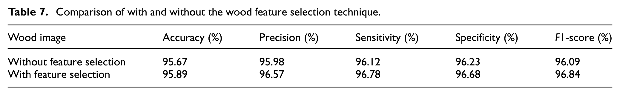
Impact of feature selection: Feature selection plays an important role in improving the performance of the wood surface image classification model, as shown in the specific figures. Without feature selection, the Accuracy reached 95.67%. Still, when feature selection was applied, the Accuracy increased to 95.89%, which is an improvement of 1.01%, showing that the model is more accurate when focusing on important features. Similarly, the Positive Precision also improved from 95.98% to 96.57%, an improvement of 0.59%, which helps reduce the error when classifying positives. The Sensitivity-Recall of the model increased from 96.12% to 96.78%, corresponding to an improvement of 0.66%, showing that the model is more sensitive in correctly detecting the truly positive samples. In terms of Specificity, without feature selection, the value reaches 96.23%, and with feature selection, it increases to 96.68%, which is an improvement of 0.45%, which helps to reduce the misclassification of negative cases. Finally, the F1-score also increases from 96.09 to 96.84, an improvement of 0.58%, showing a better balance between Precision and Sensitivity. These results demonstrate that feature selection can significantly improve the performance of the classification model (shown in Table 7).

Table 7.

Comparison of with and without the wood feature selection technique.

Wood image	Accuracy (%)	Precision (%)	Sensitivity (%)	Specificity (%)	F1-score (%)
Without feature selection	95.67	95.98	96.12	96.23	96.09
With feature selection	95.89	96.57	96.78	96.68	96.84

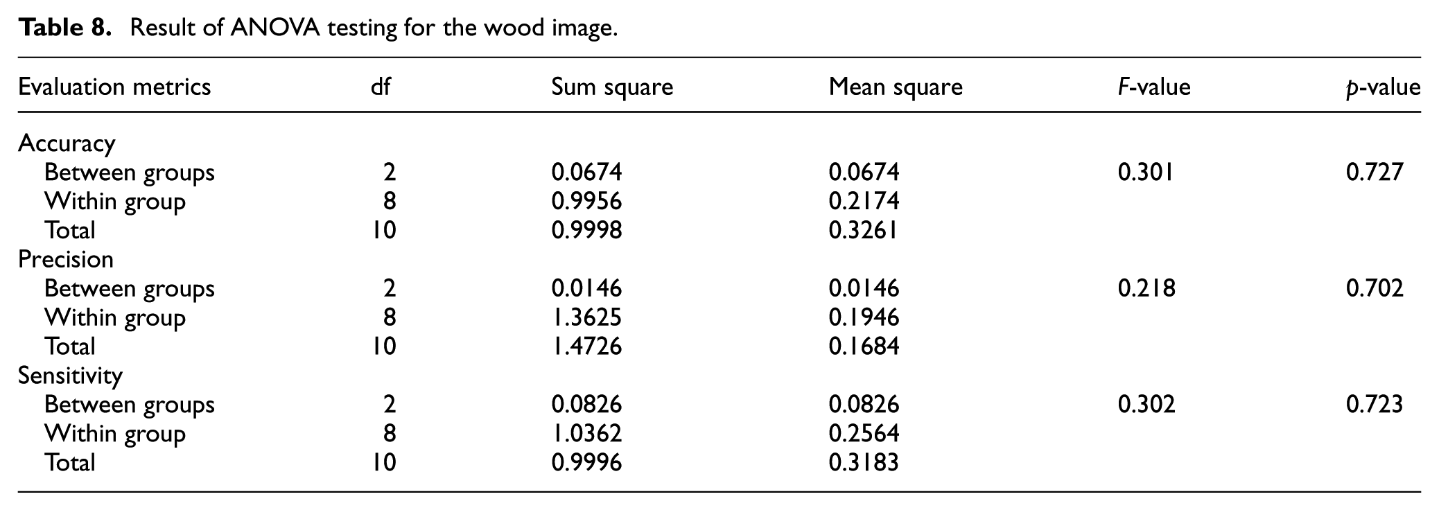
Statistical analysis: The ANOVA analysis results show that there is no significant statistical difference between the data groups based on the Accuracy, Precision, and Sensitivity indices. All p-values are greater than 0.05, which indicates that the mean values of the groups are considered equal. This result shows that the proposed method is stable when applied to different data groups, and also confirms that the method can be applied consistently without being greatly affected by the fluctuation of data within groups (shown in Table 8).

Table 8.

Result of ANOVA testing for the wood image.

Evaluation metrics	df	Sum square	Mean square	F-value	p-value
Accuracy
Between groups	2	0.0674	0.0674	0.301	0.727
Within group	8	0.9956	0.2174
Total	10	0.9998	0.3261
Precision
Between groups	2	0.0146	0.0146	0.218	0.702
Within group	8	1.3625	0.1946
Total	10	1.4726	0.1684
Sensitivity
Between groups	2	0.0826	0.0826	0.302	0.723
Within group	8	1.0362	0.2564
Total	10	0.9996	0.3183

Limitations of the proposed framework: One limitation of the proposed architecture is that it does not deal with image noise; however, this does not significantly affect the overall performance of the method. The paper discusses image noise filtering techniques such as Conservative smoothing, Gaussian smoothing, Unsharp filtering, Median filtering, and Frequency filtering, which help to improve the image quality while preserving important details. Additionally, to improve the performance of the classifier, optimization techniques such as hyper-search and Bayesian Optimization are used to find the best parameters, thereby improving the overall performance of the algorithm.

ROC-AUC result analysis

The graph shows the ROC curve, which is used to evaluate the performance of the classification model in recognizing wood defects (Figure 9). The horizontal axis represents the false positive rate, while the vertical axis represents the true positive rate. Each colored curve in the graph corresponds to a different type of wood defect, accompanied by an AUC value that indicates how accurately the model distinguishes that type of defect. The black diagonal line represents the random prediction model with AUC = 0.5, so the further the curves are from the diagonal, the more accurate the model is. Most of the defect types have AUC values greater than 0.85, indicating that the model performs well. Among them, the “blue stain” type has an AUC = 0.990, indicating near-perfect recognition, while “crack” and “marrow” also have AUCs above 0.96, indicating very high accuracy. The “knot missing” type has the lowest AUC (0.800), indicating that the model still needs further improvement in this group. Overall, the model has high reliability and is completely suitable for application in automatic wood defect classification.

Figure 9.

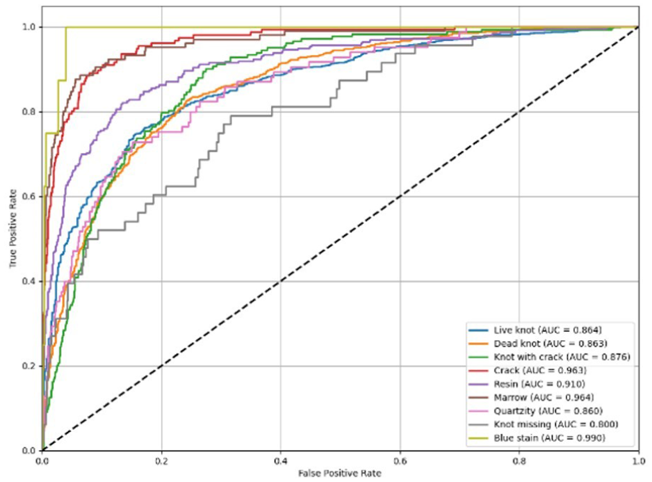
AUC analysis chart.

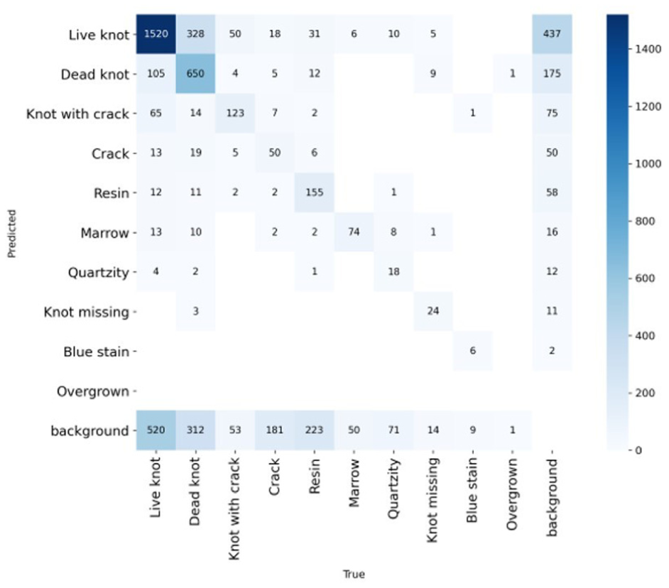
Wood surface image classification confusion matrix analysis

The above graph is a confusion matrix, which is used to evaluate the prediction results of the wood defect classification model (Figure 10). The horizontal axis shows the actual values, while the vertical axis shows the values predicted by the model. The main diagonal cells (from top left to bottom right) show the number of samples that the model predicted correctly, while the off-diagonal cells show the cases where the model predicted incorrectly. The matrix shows that the model performed best with types such as “Live knot” (1520 correct samples), “Dead knot” (650 correct samples), and “Resin” (155 correct samples), demonstrating good ability to recognize common types of defects. However, there are still some errors, for example “Live knot” is sometimes mistaken for “Dead knot” or “background,” and “Dead knot” is mistaken for “background” 175 times. Overall, the model has good accuracy but still needs improvement in its ability to distinguish between similar-shaped defects, especially between knots and background. This shows that the model performs well, but there is still room for improvement by increasing the training data or fine-tuning the image features.

Figure 10.

Confusion matrix analysis chart.

Ablation research analysis

To assess the individual contributions of each component in the CNN–LPMPSO–GATVAE framework, future work should include ablation studies (Table 9). This involves comparing the performance of simplified variants such as: (CNN alone, CNN + LPMPSO, CNN + GATVAE, and the full integrated model. Such an analysis would offer clear empirical evidence of how each module enhances overall performance and justify its inclusion in the proposed architecture. Because the problem is formulated as a multi-objective optimization, the Pareto solution set (PF) is maintained in the LPMPSO Global Archive to represent the trade-offs between the KKM and Ratio Cut objectives. From this PF, the final solution is selected based on modularity and classification performance on the validation set, ensuring a balance between structural coherence and practical accuracy. This selection strategy avoids extreme solutions and reflects the optimal configuration with practical application.

Table 9.

Ablation study on wood surface dataset.

Model variant	Accuracy (%)	Precision (%)	Sensitivity (%)	Specificity (%)	F1-score (%)
CNN only	93.56	92.83	93.71	93.12	93.24
CNN + LPMPSO	94.78	94.12	94.89	94.33	94.45
CNN + GATVAE	95.36	94.91	95.47	95.01	95.18
CNN + LPMPSO + GATVAE	95.89	95.79	96.02	96.89	96.84

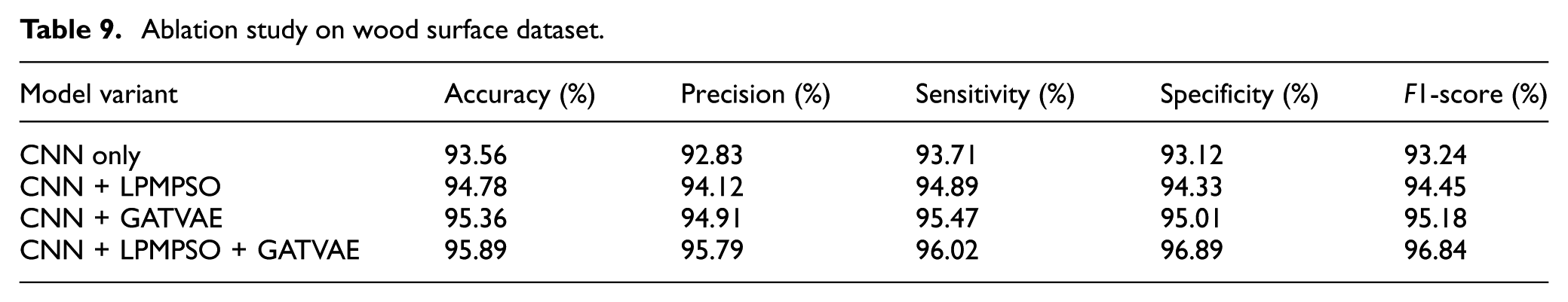
The above results Table 9 shows the performance of the model variants in the problem of wood defect classification. It can be seen that the CNN + LPMPSO + GATVAE model achieved the best results with an accuracy of 95.89%, F1-score of 96.84%, and Precision, Sensitivity, and Specificity indexes all above 95%. In comparison, the CNN-only model gave the lowest performance (Accuracy 93.56%), proving that the addition of optimization methods such as LPMPSO and GATVAE significantly improved the learning and classification ability. Specifically, when adding LPMPSO, the accuracy increased from 93.56% to 94.78%; when combining GATVAE, it continued to reach 95.36%; and when combining both, the model achieved the highest performance. This shows that the integration of optimization techniques and advanced deep learning models helps the CNN model to exploit data features more effectively, reduce prediction errors, and improve reliability in wood defect recognition. The difference in the accuracy of the CNN model in Tables 6 and 9 stems from the different evaluation contexts. Specifically, the 95.24% value in Table 6 is reported in the overall comparative experiment, where the CNN was fully trained and fine-tuned using the same data preprocessing procedure. Meanwhile, the 93.56% value in Table 9 belongs to the ablation study, where the CNN was evaluated in a minimalist configuration (CNN-only) to analyze the contribution of each component. We have added this explanation to avoid confusion and ensure consistency in the interpretation of the results.

Conclusion

This study proposed a novel hybrid deep learning architecture—CNN–LPMPSO–GATVAE—to tackle the complex problem of wood surface defect classification. The framework integrates convolutional neural networks for hierarchical feature extraction, a label-propagation-based multi-objective particle swarm optimization (LPMPSO) for optimal feature selection, and a graph attention variational autoencoder (GATVAE) for structure-aware representation learning. Notably, the model introduces a closed-loop feedback mechanism between GATVAE and LPMPSO, enabling mutual refinement of embeddings and optimization strategies—a unique contribution not seen in prior studies. The model’s conceptual deployment within a smart factory pipeline further demonstrates its feasibility for industrial-scale automation.

Experimental results on a comprehensive dataset of 20,027 annotated images confirm the effectiveness of the proposed approach. The model achieved 95.89% accuracy, 95.79% precision, 96.02% sensitivity, and 96.84% F1-score, outperforming conventional and deep learning baselines such as CNN, CheXNet, and SVM. The integration of LPMPSO led to significant improvements in model interpretability, while GATVAE enhanced the model’s ability to represent complex spatial features. These gains underline the synergy between graph-based representation learning and evolutionary feature optimization. The architecture demonstrates strong robustness, with practical applicability in real-time quality inspection scenarios in wood manufacturing (Figure 11).

Figure 11.

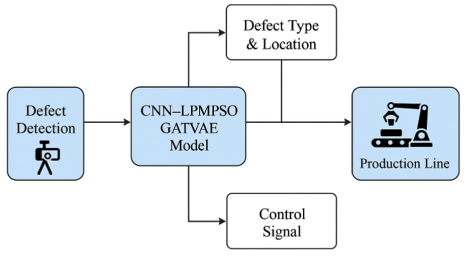
Conceptual deployment in a smart factory.

However, several limitations remain. Beyond the omission of image noise removal, the proposed method has several additional limitations that merit deeper discussion. First, the computational complexity is relatively high due to the integration of CNN, LPMPSO, and GATVAE, yet no concrete analysis of training or inference time is provided. Second, all evaluations were conducted on a single dataset sourced from a uniform acquisition environment, which limits the generalizability of the model. Third, the paper lacks direct comparisons with recent state-of-the-art models such as HaloAE, NDP-Net, and LafitE, which have demonstrated strong performance in industrial image analysis. Lastly, standard deviations of evaluation metrics are not reported, making it difficult to assess the model’s robustness across different trials. These aspects represent important directions for improvement in future studies.

One of the shortcomings of the proposed architecture is that we have missed out on removing image noise. However, this does not significantly affect the performance of our proposed method. Image noise can be removed using techniques such as Conservative smoothing, is helps to retain important details in the image while reducing noise. Gaussian smoothing uses a Gaussian distribution function to reduce noise. Unsharp filtering enhances the edges in the image to improve sharpness. Median filtering performs the average of neighboring pixels to smooth the image. Median filtering removes noise by replacing pixel values with the median value of the neighborhood. Frequency filtering separates high and low-frequency components to improve image quality. Additionally, to improve the performance of the classifier, many optimization techniques, such as the search method Search for the best parameters in the parameter space. Hyper-search optimizes the hyperparameters by testing many different configurations. Bayesian Optimization uses statistical methods to efficiently search for optimal parameters. These techniques can not only improve image quality but also enhance the overall performance of the proposed algorithm.

Future work will focus on (1) incorporating advanced denoising filters into the preprocessing stage, (2) conducting thorough ablation studies of individual model components, (3) performing evaluations on diverse datasets, and (4) optimizing the architecture for deployment on edge hardware platforms. These directions aim to enhance both the theoretical robustness and industrial readiness of the proposed framework.