A temperature compensation method for piezoresistive pressure sensors based on multi-strategy fusion improved dung beetle optimization algorithm

Abstract

To enhance the measurement accuracy of piezoresistive pressure sensors across a wide range of pressures and temperatures, this study proposes a temperature compensation model based on a Multi-strategy Fusion Improved Dung Beetle Optimization (MSDBO) algorithm. The model addresses three critical limitations of the traditional Dung Beetle Optimizer (DBO): (1) random population initialization that hinders effective environmental exploration, (2) a linear boundary convergence factor that weakens the global-local balance, and (3) susceptibility to local optima. To overcome these challenges, First, Maximin Latin Hypercube Sampling (MLHS) ensures uniform population distribution, enhancing convergence and compensation accuracy. Second, a nonlinear boundary convergence factor improves global search capability and accelerates convergence. Third, a dual-strategy combining beetle somersault foraging with adaptive Gaussian-Cauchy mutation prevents entrapment in local optima while boosting optimization capacity. The proposed MSDBO algorithm was applied to refine the weights and thresholds in a Back-Propagation Neural Network (BPNN) temperature compensation model. Practical implementation on an STM32F407VET6-based transmitter for 0–50 MPa/−20°C−70°C piezoresistive pressure sensors: temperature compensation reduced zero drift and sensitivity drift coefficients by one and three orders of magnitude, respectively, while improving full-scale accuracy from 6.36% to 0.041%—a two-order-of-magnitude enhancement.

Introduction

Since Smith ¹ discovered the silicon piezoresistive effect in 1954, piezoresistive pressure sensors have been widely used in industrial automation, biomedicine, consumer electronics, and other fields due to their high sensitivity, small size, high reliability, and cost-effectiveness.^2,3 However, silicon-based semiconductor materials are thermally sensitive in terms of resistivity, meaning that the output of pressure sensors drifts with temperature changes, particularly in high-temperature environments commonly found in the automotive, aerospace, and petroleum and petrochemical industries. Such temperature drifts can significantly reduce the measurement accuracy of piezoresistive pressure sensors, negatively impacting the system’s high-quality operation.^4–6

Extensive research on temperature compensation methods for piezoresistive pressure sensors has been conducted by scholars. The existing temperature compensation methods can be divided into two types: hardware and software compensation methods.^7–9 In hardware compensation methods, the interference caused by temperature variations is mitigated by modifying the hardware circuit, and zero drift and sensitivity drift are usually compensated separately. For example, De Bruyker and Puers ¹⁰ used on-chip heaters and temperature sensing electrodes to form a constant temperature control circuit, thereby eliminating the dependence of pressure sensors on ambient temperature; Wang et al. ¹¹ successfully fabricated a piezoresistive pressure sensor through a high-temperature packaging process, achieving good accuracy and stability through the use of circuits for compensating the sensitivity and deviation temperature coefficients; Some scholars designed temperature compensation circuits using specialized temperature drift compensation chips such as MAX1452 and NSA2860 to reduce the impact of temperature change on the output accuracy of pressure sensors.^12,13 Considering the shortcomings of hardware compensation methods (e.g. difficulty in adjustment, high production costs, and limited compensation accuracy), software compensation—a more flexible and convenient approach that obtains compensation values via numerical calculation and machine learning—is more widely adopted in practical applications. Ali et al. ⁵ proposed a polynomial-based adaptive digital temperature compensation method for the application of piezoresistive pressure sensors in automobiles. Shu et al. ¹⁴ introduced a bilinear interpolation method to compensate for pressure deviation, which improved the full-scale measurement accuracy from 21.2% to 0.1%. Wang et al. ¹⁵ proposed a temperature compensation method based on Newton interpolation and cubic spline interpolation to reduce temperature drift. These numerical calculation-based compensation methods struggle to accurately model the complex interplay between temperature and pressure. Moreover, handling a broad temperature spectrum and a wide pressure measurement range to pursue higher compensation accuracy can lead to exponential growth in data volume.

Machine learning (ML), as an advanced data analysis tool, simulates the learning process of the human brain, enabling the extraction of features, discovery of patterns, and making accurate predictions or decisions from complex data.^16–18 Machine learning compensation methods can effectively solve the problems in numerical calculations mentioned above. BP neural networks, with their excellent nonlinear fitting and adaptive learning capabilities, can accurately capture nonlinear and abrupt changes based on sensor output or new environmental data changes, and automatically update strategies to suit individual sensors. However, the efficiency of temperature compensation depends on the set values of neuron connection weights and thresholds. Therefore, how to use intelligent optimization algorithms to optimize weights and thresholds for efficient temperature compensation has become a research hotspot in the field of piezoresistive pressure sensors. Wang et al. ¹⁹ proposed a backpropagation neural network method based on the Whale Optimization Algorithm to replace the traditional least squares method for temperature compensation, resulting in a significant 0.25% reduction in error. Ye et al. ²⁰ used a genetic algorithm (GA) to remedy two deficiencies of BP neural networks, which are slow convergence and a tendency to fall into local optima, significantly improving the calibration accuracy of pressure sensors. Wu and Jiang ²¹ proposed a BP neural network temperature compensation model based on particle swarm optimization and the Levenberg-Marquardt algorithm (PSO-LM-BP), effectively suppressing the temperature drift of pressure sensors. Although the above algorithms can improve the performance of BP neural networks to a certain extent and reduce the influence of temperature change on pressure sensors, their application is limited by several shortcomings. Data obtained in practical applications show that when piezoresistive pressure sensors are applied in complex scenarios, such as oil wells and aircraft/spacecraft, involving nonlinear mapping of high-temperature and high-pressure parameters, these algorithms generally suffer from problems such as the tendency to fall into local optima, limited optimization accuracy, and slow convergence, making it difficult to efficiently find the optimal combination of BP neural network weights and thresholds. Consequently, the effect of temperature compensation is not satisfactory, and it fails to meet the requirements for high-precision pressure measurement.

Based on the above analysis, we developed an improved multi-strategy fusion dung beetle optimization algorithm (MSDBO) by reforming the population initialization method, adjusting the beetle position updating mechanism, and incorporating a late-stage mutation mechanism into the traditional DBO. The MSDBO-BP neural network-based temperature compensation model for piezoresistive pressure sensors effectively optimizes the BP neural network weights and thresholds while balancing global search and local exploration capabilities. This approach prevents the DBO algorithm from converging to local optima, significantly enhancing the temperature compensation accuracy of piezoresistive pressure sensors. To verify the performance of the MSDBO-BP temperature compensation model and evaluate its superiority against the traditional BP and seven other BP-based temperature compensation models optimized by meta-heuristic algorithms, we conducted multiple simulations and experiments. The results demonstrate that MSDBO-BP achieves superior temperature compensation accuracy and strong generalization ability over a broad pressure range and a wide temperature range.

Temperature drift characteristics of piezoresistive pressure sensors

The core principle of piezoresistive pressure sensors is based on the piezoresistive effect of semiconductor materials. ⁷ This sensor uses diffusion or ion implantation methods to fabricate four nearly equal piezoresistors on a silicon diaphragm and arranges them in a Wheatstone bridge structure, As shown in Figure 1.

Figure 1.

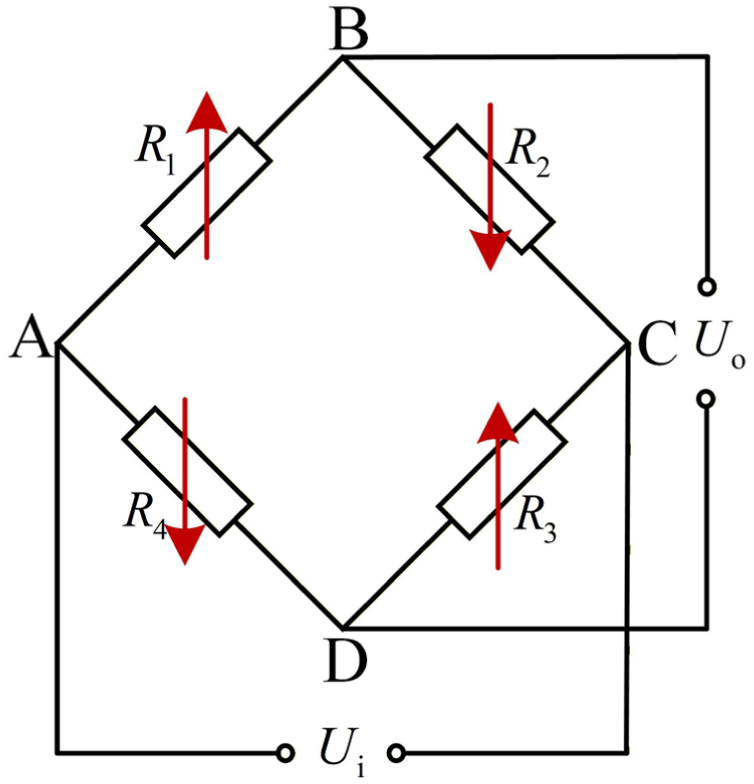
Working principle of piezoresistive pressure sensor.

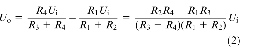
When the diaphragm is subjected to pressure, it undergoes elastic deformation, causing lattice structure changes in the piezoresistors located in different areas: R₁ and R₃ are in the compression zone, and their resistance values increase; R₂ and R₄ are in the tension zone, and their resistance values decrease. Under the excitation of an external voltage, the precise measurement of pressure is achieved based on the proportional relationship between the unbalanced voltage output by the bridge and the pressure. The calculation of the resistance values of each bridge arm and the output voltage Uo is shown in equations and.

$$\{\begin{array}{c}{R}_1=R_3=R_0+\mathrm{\Delta }{R}_{\mathrm{T}}+\mathrm{\Delta }{R}_{\mathrm{P}}\hfill \\ \multicolumn{1}{c}{R_2=R_4=R_0+\mathrm{\Delta }{R}_{\mathrm{T}}-\mathrm{\Delta }{R}_{\mathrm{P}}}\end{array}$$

(1)

$$U_{\mathrm{o}}=\frac{R_4{U}_{\mathrm{i}}}{R_3+R_4}-\frac{R_1{U}_{\mathrm{i}}}{R_1+R_2}=\frac{R_2{R}_4-R_1{R}_3}{(R_3+R_4)(R_1+R_2)}{U}_{\mathrm{i}}$$

(2)

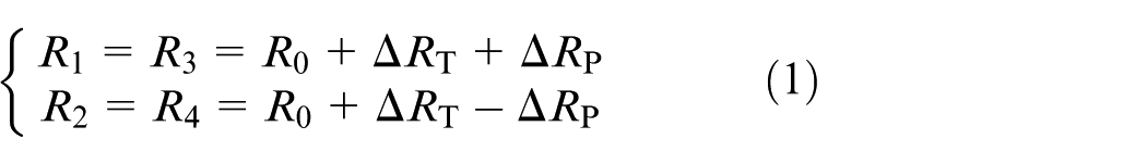
Where R₁, R₂, R₃, and R₄ are the initial values of the four resistors on the bridge arms, R₀ is the resistance value of the bridge arm at 0°C, ΔR_P is the resistance change caused by external pressure, and ΔR_T is the resistance change caused by variations in ambient temperature.

From equations and, it can be seen that a change in temperature will affect the resistance value of the bridge arm, and thus cause a temperature-related voltage offset in the output U_o.

In practical pressure measurement, the accurate response capability of a sensor to pressure changes directly depends on its sensitivity, which is a core performance indicator. For silicon material, 1 + 2 μ ≪ πE, so the sensor sensitivity coefficient K is calculated as shown in the equation ²² :

$$K=(1+2\mu )+\pi E\approx \pi E=Z{T}^{-V}$$

(3)

where μ is the Poisson’s coefficient of the silicon material, π is the longitudinal piezoresistive coefficient of the silicon material, E is the elastic modulus of the material, Z and V are constants related to the concentrations of the silicon material and impurities, respectively, and T is the ambient temperature.

It can be seen from equation that the sensitivity K of the pressure sensor decreases with the increase of temperature T, thereby resulting in a decrease in the output accuracy of the sensor. In practice, the sensitivity coefficient is defined as the ratio of the change in output voltage to the change in pressure, which is typically determined through experimental measurement of this ratio. Sensor accuracy is susceptible to various factors, including uneven doping of piezoresistors, process deviations in Wheatstone bridges, mechanical stress, electromagnetic interference, and long-term aging. Among these influencing factors, once the manufacturing process and external mechanical conditions are fixed, temperature variations during practical operation will cause changes in the piezoresistive coefficient and elastic modulus of silicon materials, making temperature the most significant factor affecting accuracy. Therefore, temperature compensation measures need to be taken to ensure the accurate output of data in a wide-temperature environment.

MSDBO-BP temperature compensation model

Temperature compensation model based on BP neural network

The BP neural network is a three-layer feedforward architecture trained using the error backpropagation algorithm, consisting of input, hidden, and output layers. With high adaptability, self-learning ability, and fault tolerance, the network effectively solves intricate nonlinear mapping problems. The range of the number of nodes in the hidden layer can be determined according to the empirical formula $\mathrm{k}=\sqrt{\mathrm{m}+\mathrm{n}}+h$ , where m = 2(number of inputs: pressure and temperature), n = 1(number of outputs: compensated pressure), and h is an integer within the range of 1–10. To simplify the structure of the network model and facilitate its implementation in engineering, the number of nodes in the hidden layer was finally determined to be six through experiments conducted in this study. As shown in Figure 2, the measured pressure P and the ambient temperature T serve as the inputs $\mathit{X}=[P,T{]}^{\top }$ of the temperature compensation model of the piezoresistive pressure sensor based on the BP neural network. After a series of calculations involving the weight matrix W ₁ (of dimension 2 × 6) from the input layer to the hidden layer and threshold vector b ₁  = (b₁₁, b₁₂,…, b₁₆) as well as the weight matrix W ₂ (of dimension 6 × 1) from the hidden layer to the output layer and threshold value b₂₁, the post-compensation pressure value P′ is output. The mathematical formula is shown in equation.

$$\begin{array}{c}\multicolumn{1}{c}{P^{\prime }=\varphi (\sum {\mathit{W}}_{\mathit{2}}\times (f(\sum {\mathit{W}}_{\mathit{1}}\times \mathit{X}+{\mathit{b}}_{\mathit{1}})+b_{21})}\\ \multicolumn{1}{c}{=\mathrm{purelin}(\sum {\mathit{W}}_{\mathit{2}}\times (\mathrm{tansig}(\sum {\mathit{W}}_{\mathit{1}}\times \mathit{X}+{\mathit{b}}_{\mathit{1}})+b_{21})}\end{array}$$

(4)

Figure 2.

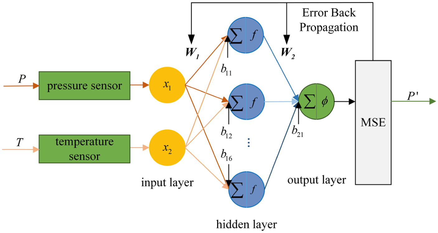
Temperature compensation model based on BP neural network for piezoresistive pressure sensors.

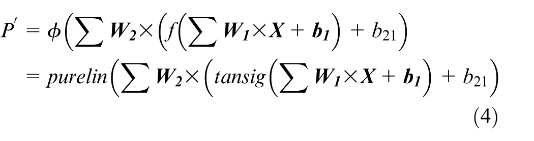
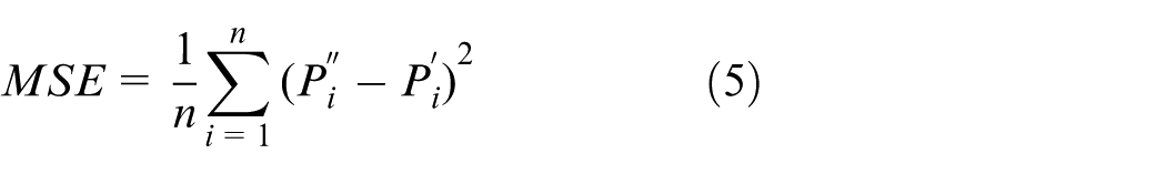
In this paper, the activation functions f and ϕ are the tansig function and purelin pure linear function respectively. The L-M algorithm is used to adjust the weights and thresholds layer by layer in reverse order to gradually reduce the mean square error (MSE) between the standard pressure P″ and the post-compensation pressure value P′ until the preset stopping condition is met. The calculation formula for MSE is shown in equation:

$$\mathrm{MSE}=\frac{1}{n}\sum _{i=1}^n{(P_i^{″}-P_i^{\prime })}^2$$

(5)

As seen in equation, the weight values W ₁ and W ₂ of the BP neural network, along with the threshold values b ₁ and b₂₁, determine the connection strength between neurons. Improper selection of these values directly affects the optimization performance and stability of the network, leading to issues such as falling into local optima and slow convergence. The impact of poorly selected weight and threshold values is particularly significant in high-temperature and high-pressure environments (such as oil wells and aircraft/spacecraft) characterized by a wide temperature compensation range, high nonlinear complexity, and strong interference. To achieve high-precision pressure measurement, it is essential to optimize the combination of weights and thresholds for the BP temperature compensation model.

DBO algorithm

The DBO algorithm is a metaheuristic algorithm proposed by Xue and Shen ²³ in 2022, which divides the dung beetles in a beetle population into five categories based on behaviors: ball rolling, dancing, breeding, foraging, and stealing. Its stability and simplicity provide advantages over other metaheuristic optimization algorithms.

Position updating of ball rolling dung beetles

When there are no obstacles on the road, a ball-rolling beetle utilizes the sun to navigate, ensuring that the dung ball rolls in a straight path. Natural factors such as light intensity and wind can influence its travel route. The position update can be calculated using equation:

$$\begin{array}{c}\multicolumn{1}{c}{x_i(t+1)=x_i(t)+\lambda \times a\times x_i(t-1)+b\times \mathrm{\Delta }x,}\\ \multicolumn{1}{c}{\mathrm{\Delta }x=|x_i(t)-X_{\mathrm{worst}}|}\end{array}$$

(6)

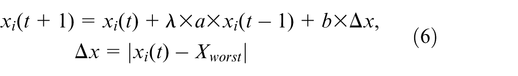
where t is the current iteration count, and x _i (t) represents the position of the i-th beetle in the t-th iteration, λ is a natural coefficient assigned a value of −1 or 1. A random number η∈ (0, 1) is introduced to control the switching of the dung beetle’s behavioral modes: when η < 0.9, λ = 1, indicating that the natural environment does not affect the original direction, and the dung beetle continues rolling the ball in the initial direction; when η ≥ 0.9, λ = −1, meaning the dung beetle encounters an obstacle and performs a dancing behavior, resulting in a significant change in direction. a is the deflection coefficient, b is a constant, according to Ref., ²³ a∈(0,0.2), b∈(0,1) denotes the optimal parameter range for the DBO algorithm, which can accurately balance the exploration and exploitation capabilities of the algorithm. It effectively avoids problems such as search oscillation, convergence stagnation, or trapping in local optima caused by parameter values deviating from this range, thereby providing a fundamental guarantee for the stable and efficient optimization of the DBO algorithm. X _worst is the global worst position, and Δx is used to simulate variations in light intensity.

Position updating of dancing dung beetles

When a dung beetle encounters an obstacle that blocks its path, it relocates itself to find a new route before continuing to roll the dung ball. The position update can be calculated using equation:

$$x_i(t+1)=x_i(t)+\tan (\theta )|x_i(t)-x_i(t-1)|$$

(7)

where θ is the deflection angle within the range (0,π])|x _i (t)-x _i (t–1)| is the position difference of the i-th beetle between the t-th and (t + 1)-th iterations. It can be observed that the position update of a dung beetle is closely related to both current and historical information.

Position updating of dung beetle egg ball

For progeny security, dung beetles select optimal position sites. The boundary selection strategy of the DBO algorithm can be used to model the spawning area of female dung beetles. As shown in Figure 3.

Figure 3.

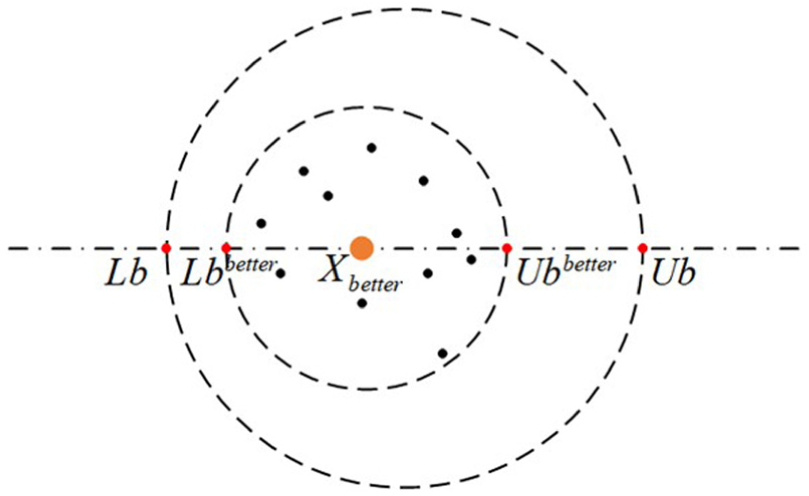
Conceptual model of boundary selection strategy.

The orange dot X _better represents the local optimal position of the current beetle, while the black dot represents the brooding ball. The area between the lower limit Lb and upper limit Ub of the BP weight threshold is the initial spawning area of the female beetle. The boundary convergence factor R changes with the increase in iteration count t, updating the lower limit Lb^better and upper limit Ub^better of the spawning area. The mathematical expression for the spawning area is shown in equation:

$$\begin{array}{c}\multicolumn{1}{c}{L{b}^{\mathrm{better}}=max(X_{\mathrm{better}}\times (1-R),\mathrm{Lb}),}\\ \multicolumn{1}{c}{U{b}^{\mathrm{better}}=min(X_{\mathrm{better}}\times (1+R),\mathrm{Ub})}\\ \multicolumn{1}{c}{R=1-\frac{t}{T_{max}}}\end{array}$$

(8)

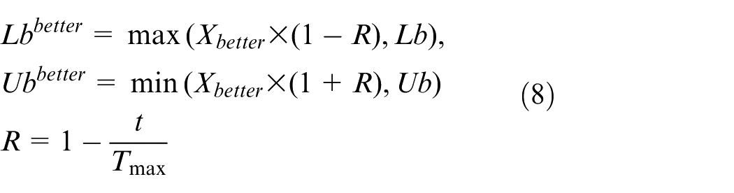
Once the spawning area is identified, the female beetle lays eggs inside a brood ball in that specific area, and the egg ball’s coordinates are then updated according to equation:

$$\begin{array}{c}\multicolumn{1}{c}{F_i(t+1)=X_{\mathrm{better}}+{\mathit{A}}_{\mathit{1}}\times (F_i(t)-L{b}^{\mathrm{better}})}\\ \multicolumn{1}{c}{+{\mathit{A}}_{\mathit{2}}\times (F_i(t)-U{b}^{\mathrm{better}})}\end{array}$$

(9)

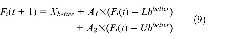
where F_i(t) is the position of the i-th brooding ball at the t-th iteration, A ₁ and A ₂ are two independent random vectors of size 1 × D, and D represents the optimization dimension. The structure of the BP temperature compensation model proposed in this paper is 2-6-1, and D is the number of weight and threshold values that need to be optimized (which is 25).

Position updating of foraging dung beetles

To simulate the foraging behavior of young dung beetles after hatching from egg balls, the DBO algorithm establishes the optimal foraging area. The definition of the area boundary and the position update of young dung beetles are given in equation:

$$\begin{array}{c}\multicolumn{1}{c}{L{b}^{\mathrm{best}}=\max (X_{\mathrm{best}}\times (1-R),\mathrm{Lb})}\\ \multicolumn{1}{c}{U{b}^{\mathrm{best}}=\min (X_{\mathrm{best}}\times (1+R),\mathrm{Ub})}\\ \multicolumn{1}{c}{x_i(t+1)=x_i(t)+B_1\times (x_i(t)-L{b}^{\mathrm{best}})}\\ \multicolumn{1}{c}{+{\mathit{B}}_{\mathit{2}}\times (x_i(t)-U{b}^{\mathrm{best}})}\end{array}$$

(10)

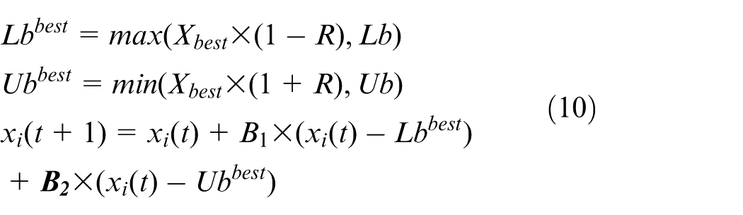
where X _best represents the global optimal foraging location, Lb^best and Ub^best respectively represent the lower and upper limits of the optimal foraging area, B₁ is a random number that follows a normal distribution, and B ₂ is a random vector within the range (0,1).

Position updating of thief dung beetles

In the beetle population, some thief beetles steal food. As seen in equation, X _best is the global optimal foraging location, and the DBO algorithm takes X _best as the best place for the thief beetle to steal food. The position update of the thief beetle can be calculated using equation:

$$\begin{array}{c}\multicolumn{1}{c}{x_i(t+1)=X_{\mathrm{best}}+h\times \mathit{G}\times (|x_i(t)-X_{\mathrm{better}}|}\\ \multicolumn{1}{c}{+|x_i(t)-X_{\mathrm{best}}|)}\end{array}$$

(11)

where G is a 1 × D random vector, normally distributed, and h represents a constant value.

From the iterative optimization processes of the five types of beetle individuals described above, the optimization ability of the DBO algorithm depends on the initial population position, position updating parameters, and the quality of individual positions. The randomness of DBO population initialization and the fixed iteration order can easily lead to the following undesirable situation: the algorithm fails to achieve sufficient global exploration and gets stuck in local optima during the iteration process. When DBO is used to deal with complex nonlinear relationships in the wide temperature range of piezoresistive pressure sensors, it may only find a locally optimal combination of weight and threshold values, failing to provide a high-quality temperature compensation effect. Based on this analysis, we improved the DBO algorithm by incorporating a multi-strategy fusion approach, improving global search ability by changing the population initialization method, adjusting the beetle position updating mechanism, and adding a mutation mechanism in the later stage of iteration.

DBO algorithm multi-strategy fusion improved DBO optimization algorithm

Improving beetle position initialization using MLHDS

The traditional DBO algorithm generates a random number to initialize the population position. As a result, the quality inconsistency between the initial beetle positions prevents the algorithm from traversing all positions in the solution space, degrading optimization performance and affecting convergence speed. Latin hypercube sampling (LHS) is an effective method for simulating random sampling from the distribution of multidimensional parameters, characterized by good uniformity, a decoupling effect, and diversity. ²⁴ However, due to the randomness of the sample sequence, sample points are prone to linear or quasi-linear distribution, resulting in unsatisfactory spatial filling results. To address this issue, this paper introduces the concept of maximum and minimum values for optimization on the basis of LHS. Taking a 5 × 5 space as an example, the process of selecting sample points is as follows:

• 1) As shown in Figure 4(a) Step 1, when the first sample point is randomly selected from the P₁-th point of the (i = 4)-th row, the distances between the P₁-th point and the remaining rows in the second column (which are d((1,2), P₁), d((2,2), P₁), d((3,2), P₁) and d((5,2), P₁)) are calculated. The (i = 1)-th row corresponding to the maximum distance value d((1,2), P₁) is selected to generate the second sample point P₂.

• 2) As shown in Figure 4(b) Step 2, since the existing points P₁ and P₂ occupy rows No.4 and No.1 respectively, the distances between points P₁ and P₂ and the remaining rows (No.2, No.3, No.5) in column 3 (which are d((2,3), P₁), d((3,3), P₁), d((5,3), P₁), d((2,3), P₂), d((3,3), P₂) and d((5,3), P₂)) are first calculated, and then d((2,3), P₁), and d((2,3), P₂) are compared to select the minimum distance value d((2,3), P₂) as the characteristic distance of the second row. Similarly, the characteristic distances of the third and fifth rows are determined separately (indicated by yellow lines). Finally, the characteristic distances of all rows are compared, and the (i = 5)-th row corresponding to the maximum characteristic distance value is selected to generate the third sample point P₃.

• 3) As shown in Figure 4(c) Step 3, the fourth sample point P₄ is generated using the method in step 2).

• 4) As shown in Figure 4(d) Step 4, in the fifth column, only one row (i = 2) remains to generate the fifth sample pointP₅.

Figure 4.

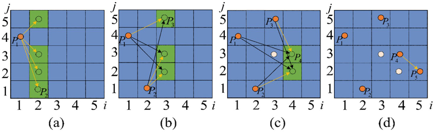
Process of sample point selection using MLHS: (a) Step 1, (b) Step 2, (c) Step 3 and (d) Step 4.

Assuming the initial positions of 500 dung beetles in a two-dimensional space are determined as a result of position initialization, Figure 5 presents the point distribution maps and three-dimensional histograms of the position initialization results obtained using the proposed MLHS method, the Rand method, and the LHS method. Evidently, the distribution of sample points generated by the MLHS method is more dispersed compared to those produced by the other two methods, striking a good balance between space-filling and uniformity. Consequently, the dung beetle population generated through this method exhibits greater uniformity and better spatial coverage, enhancing the convergence and accuracy of the temperature compensation algorithm.

Figure 5.

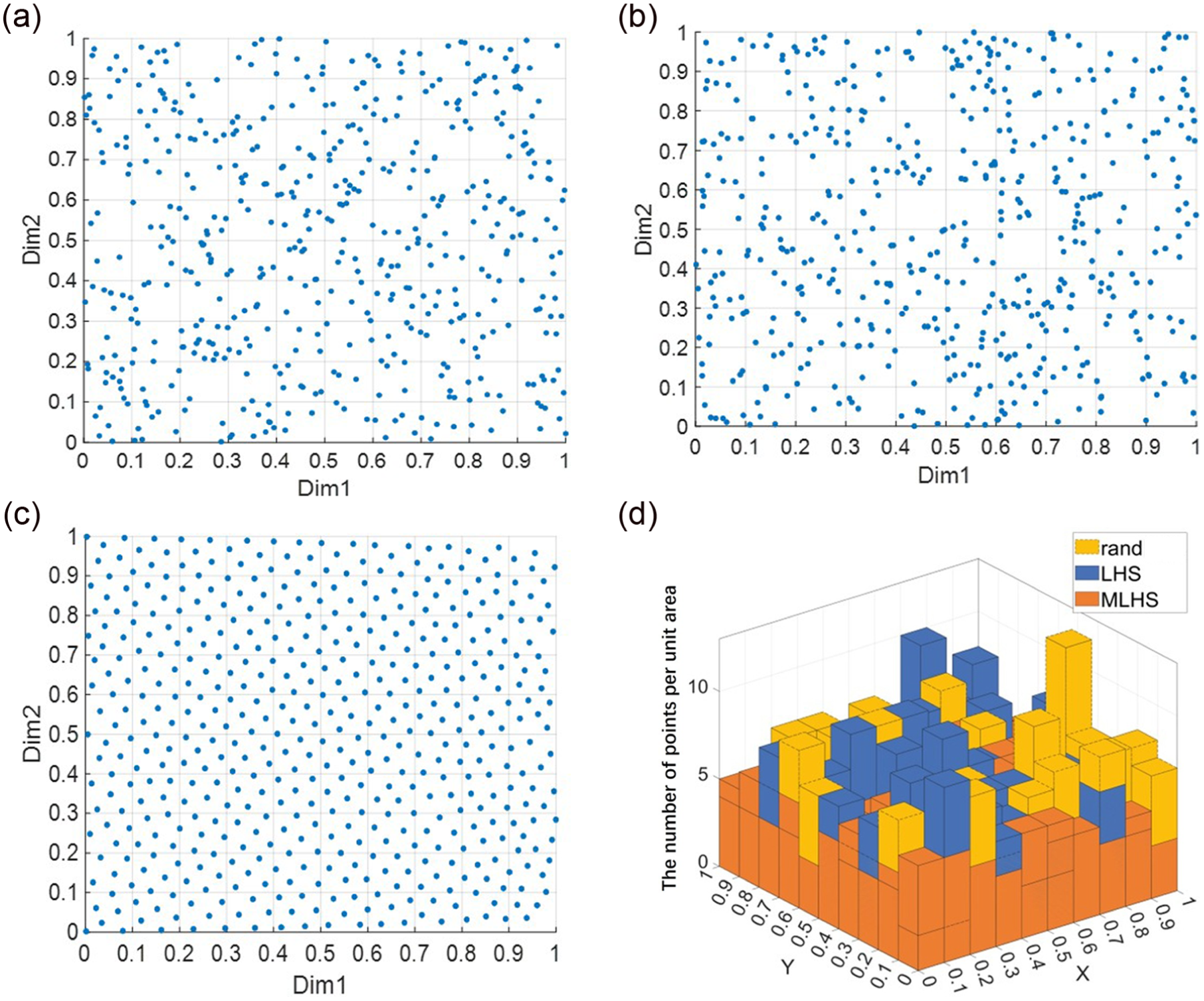
Comparison of sample points generated by Random, LHS, and MLHS: (a)the random method, (b) the LHS method, (c) the MLHS method, and (d) histograms of the sample points.

Improving the boundary convergence factor R

As seen in equation, the boundary convergence factor R of the traditional DBO algorithm decreases linearly with the increase in iteration count t, causing the spawning area to shrink uniformly. This linear change is not only unfavorable for female dung beetles to fully explore the solution space in the early stage, but also significantly slows down local exploration in the later stage. To address this issue, this paper uses the sigmoid function to improve the boundary factor R. After this enhancement, the position updating of the beetle egg ball is conducted as shown in equation. The aim is to improve the global exploration ability while maintaining good balance between local search speed and accuracy.

$$\begin{array}{c}\multicolumn{1}{c}{L{b}^{\mathrm{better}}=max(X_{\mathrm{better}}\times (1-R),\mathrm{Lb}),}\\ \multicolumn{1}{c}{U{b}^{\mathrm{better}}=min(X_{\mathrm{better}}\times (1+R),\mathrm{Ub})}\\ \multicolumn{1}{c}{R^{\prime }=1-\frac{1}{1+e^{-k(t-T_{max}/2)}}}\\ \multicolumn{1}{c}{F_i(t+1)=X_{\mathrm{better}}+{\mathit{A}}_{\mathit{1}}\times (F_i(t)-L{b}^{\mathrm{better}})}\\ \multicolumn{1}{c}{+{\mathit{A}}_{\mathit{2}}\times (F_i(t)-U{b}^{\mathrm{better}})}\end{array}$$

(12)

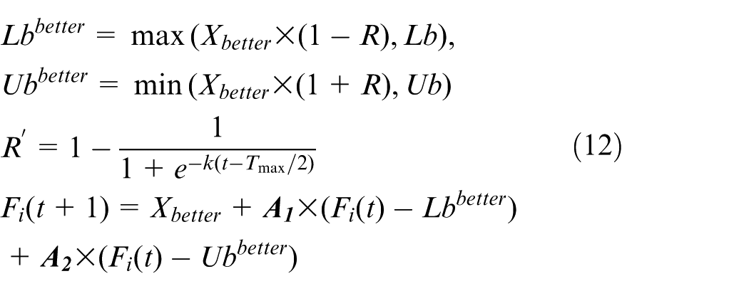
where k represents the curve steepness of the improved boundary convergence factor R’, and T_max is the maximum number of iterations. Experimental results show that the best performance can be achieved when the value of k is set to 0.1. The iteration curves of the original boundary convergence factor R and the improved boundary convergence factor R’ are shown in Figure 6.

Figure 6.

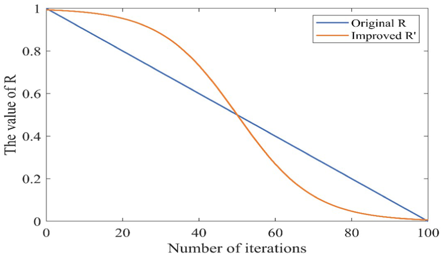
Iteration curves of original and improved boundary convergence factors.

It can be seen from Figure 6 that after replacing the boundary convergence factor R with R’, R’ decreases at a comparatively slower rate in the early stages of iteration. This allows female beetles to expand their search for egg-laying areas, thereby improving global exploration ability and increasing the likelihood of finding the optimal solution. In the middle stage of iteration, the boundary convergence factor R’ rapidly decreases to enhance local exploration ability, thus accelerating the convergence speed of the algorithm. In the later stages of iteration, R’ is maintained at a low value to ensure the stability of algorithm convergence.

Improving position updating of foraging beetles using somersault strategy

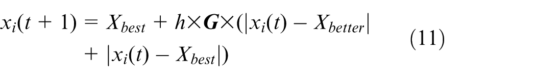
As seen in equation, when the optimal foraging area is determined, the small beetle population quickly approaches the global optimal foraging position X _best by randomly walking in a straight line. This significantly accelerates convergence, but insufficient exploration of surrounding areas can easily lead the algorithm to local optima. Inspired by the foraging behavior of manta rays, ²⁵ this paper introduces somersault foraging into the behavioral repertoire of dung beetles. To address this issue, in addition to walking in a straight line toward the global optimal foraging position X _best , a dung beetle can also use X _best as a fulcrum to gradually approach the global optimal foraging position through back-and-forth somersaulting. After this improvement, the position update of a foraging dung beetle can be calculated using equation:

$$\begin{array}{c}\multicolumn{1}{c}{x_i(t+1)=}\\ \multicolumn{1}{c}{\{\begin{array}{c}\begin{array}{cc}{x}_i(t)+S\times (r_1\times X_{\mathrm{best}}-r_2\times x_i(t)),\hfill & {\mathrm{r}}_3\le 0.5\hfill \end{array}\hfill \\ \multicolumn{1}{c}{\begin{array}{cc}\begin{array}{c}{x}_i(t)+B_1\times (x_i(t)-L{b}^{\mathrm{best}})+\hfill \\ \multicolumn{1}{c}{{\mathit{B}}_{\mathit{2}}\times (x_i(t)-U{b}^{\mathrm{best}}),}\end{array}\hfill & {\mathrm{r}}_3>0.5\hfill \end{array}}\end{array}}\end{array}$$

(13)

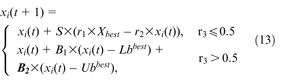
where S is the somersault factor, and r₁, r₂, and r₃ are random numbers in the range [0,1]. The somersault foraging behavior of dung beetles is illustrated in Figure 7.

Figure 7.

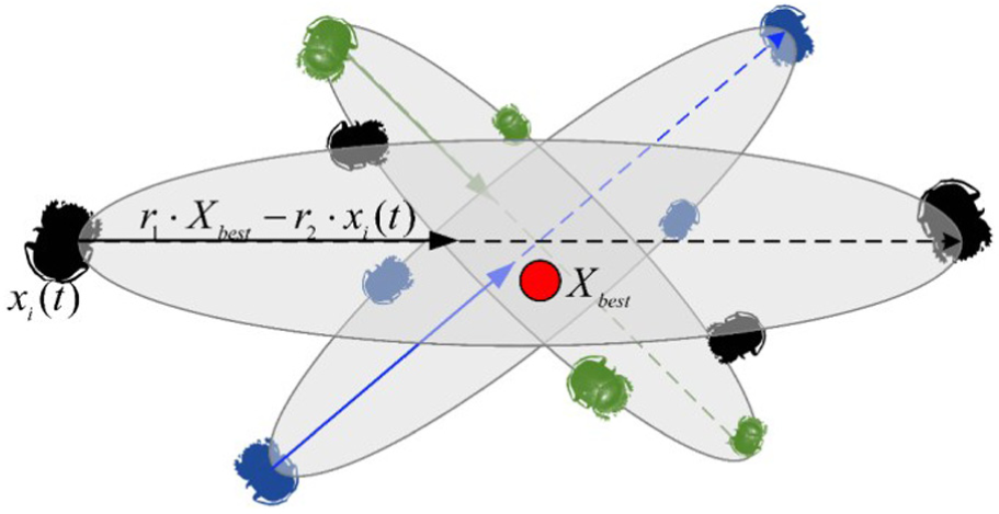
Schematic diagram of somersault foraging behavior of dung beetles.

As seen in equation and Figure 7, when a small dung beetle performs somersault foraging, its new position is always generated at a point between its current position and the symmetric point of its current position concerning the globally optimal foraging position X _best . The search area decreases as the distance between the beetle and the current global optimal foraging position X _best shortens. By combining the original foraging behavior and somersaulting, the foraging diversity and convergence of the small dung beetle are enhanced, helping the algorithm escape local optima and find the optimal combination of weight and threshold values for the BP neural network.

Adaptive Gaussian-Cauchy perturbation mutation strategy

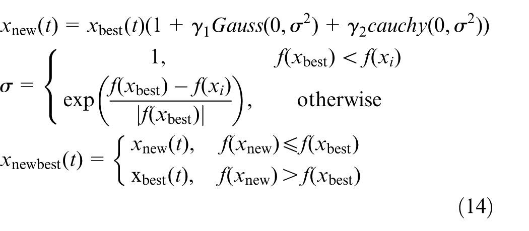
Since the DBO algorithm follows a serial iteration process, if it falls into a locally optimal solution in the early stage, beetle individuals will gradually converge toward this solution in later stages, resulting in premature convergence and low optimization efficiency. To avoid this situation, this mutation strategy to modify the optimal individual position after the iteration of the entire beetle population is completed. As shown in Figure 8, the Cauchy distribution has a higher probability of producing a two-wing distribution compared to the Gaussian distribution. This means the former is more likely to generate a wider range of random numbers that spread farther from the zero point. Therefore, the Cauchy distribution is more suitable for the early stages of iteration, as it allows beetle individuals to search the optimal area with large step sizes, increasing the probability of escaping local optima. By contrast, the Gaussian distribution is more likely to generate random numbers near zero, making it suitable for later stages. It allows beetle individuals to explore the optimal area with small steps, thus quickly converging to the optimal value. Based on the above analysis, this paper introduces a mutation operator with an adaptive dynamic weight coefficient to balance the abilities of the two distributions, ensuring a balanced trade-off between global search and local exploration abilities. After this improvement, the position update is conducted as shown in the equation:

$$\begin{array}{c}\multicolumn{1}{c}{x_{\mathrm{new}}(t)=x_{\mathrm{best}}(t)(1+{\gamma }_1\mathrm{Gauss}(0,{\sigma }^2)+{\gamma }_2\mathrm{cauchy}(0,{\sigma }^2))}\\ \multicolumn{1}{c}{\sigma =\{\begin{array}{cc}1,\hfill & f(x_{\mathrm{best}})<f(x_i)\hfill \\ \multicolumn{1}{c}{\exp \left(\frac{f(x_{\mathrm{best}})-f(x_i)}{|f(x_{\mathrm{best}})|}\right),}& \mathrm{otherwise}\hfill \end{array}}\\ \multicolumn{1}{c}{x_{\mathrm{newbest}}(t)=\{\begin{array}{cc}{x}_{\mathrm{new}}(t),\hfill & f(x_{\mathrm{new}})\le f(x_{\mathrm{best}})\hfill \\ \multicolumn{1}{c}{{\mathrm{x}}_{\mathrm{best}}(t),}& f(x_{\mathrm{new}})>f(x_{\mathrm{best}})\hfill \end{array}}\end{array}$$

(14)

Figure 8.

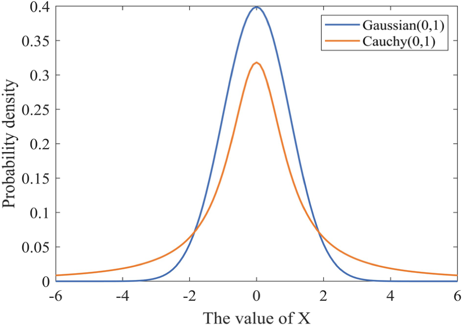
Gaussian distribution and Cauchy distribution.

where x_best(t) represents the current optimal position of the beetle individual, x_new(t) represents the individual position after mutation, and x_newbest(t) represents the final optimal position of the beetle individual, f (x_best) and f (x _i ) are the optimal and current position fitness values, respectively, σ is the standard deviation of Cauchy-Gaussian mutation, while Gauss(0,σ ² ) and Cauchy(0,σ ² ) are random numbers respectively following Gaussian and Cauchy distributions, γ₁ and γ₂ are the dynamic weight coefficients of the two distributions that are adaptively adjusted with the iteration count. The formulas for calculating γ₁ and γ₂ are shown in:

$$\begin{array}{c}\multicolumn{1}{c}{{\gamma }_1=\frac{t^2}{{T_{max}}^2}}\\ \multicolumn{1}{c}{{\gamma }_2=1-\frac{t^2}{{T_{max}}^2}}\end{array}$$

(15)

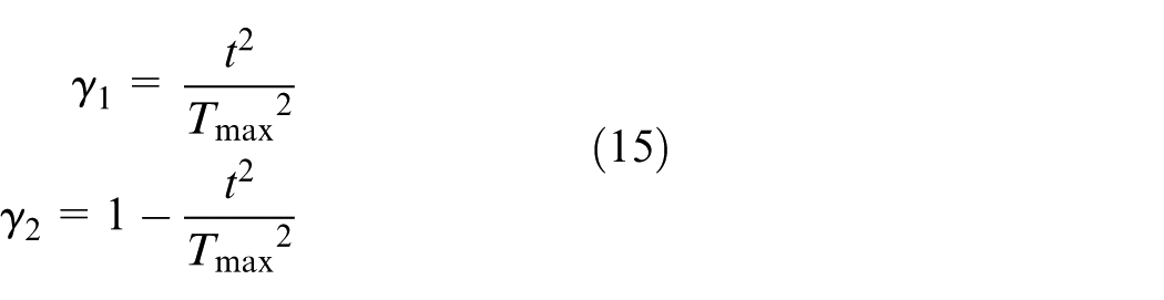
As can be seen from equations and, the best beetle individual is selected for mutation in the optimization process of the algorithm, enabling it to escape local optima. In the early stage of iteration, the Cauchy dynamic weight coefficient γ₂ is comparatively larger, so the algorithm makes use of the strong perturbation ability of Cauchy mutation to explore the entire search space. In the later stage of iteration, the Gaussian weight coefficient γ₁ increases, so the algorithm relies on Gaussian mutation to explore the local area more finely. To guarantee better optimization capability of the algorithm after disturbance, this paper proposes to introduce greedy rules. Thus, the fitness values before and after mutation disturbance are compared before deciding whether to update the optimal position.

After the above improvement strategies are implemented, the proposed MSDBO algorithm is obtained. The flowchart of MSDBO is shown in Figure 9.

Figure 9.

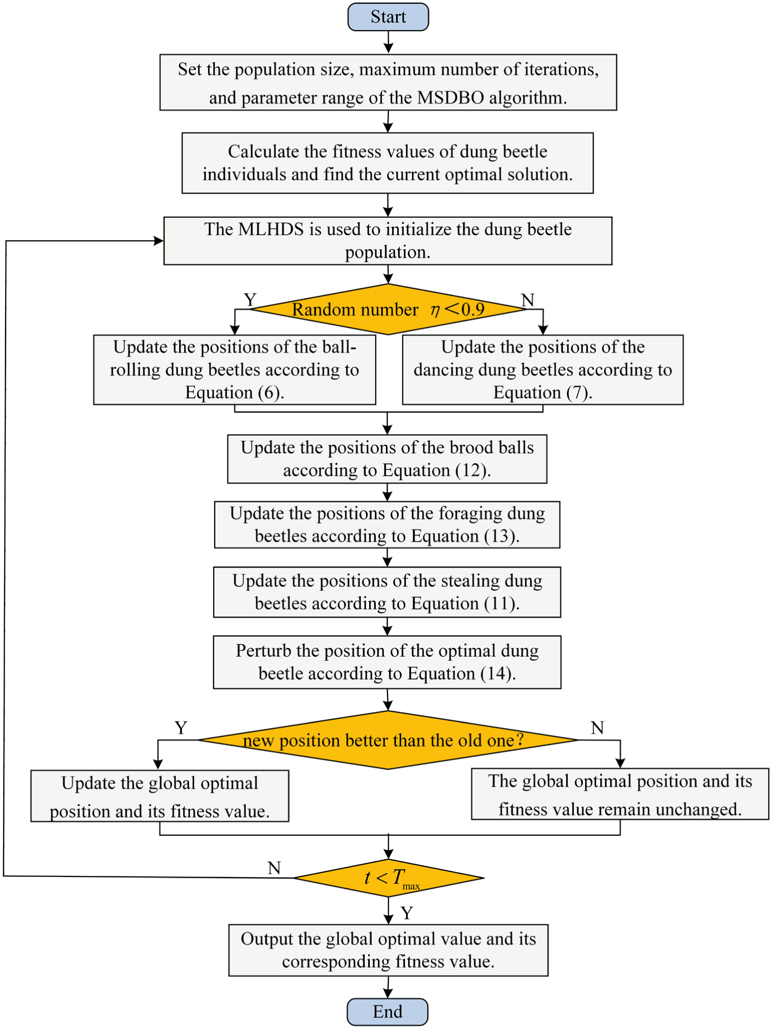
Flowchart of MSDBO algorithm.

Construction of temperature compensation model for MSDBO-BP

The MSDBO algorithm from Section 3.3 is used to find the optimal combination of weights and thresholds in the BP temperature compensation model. The optimized parameter values are then input into the BP model to achieve temperature compensation for the pressure sensor. The algorithm flow is shown in Figure 10, with the specific steps as follows:

• 1) Collect experimental data. Obtain the measured sensor pressure P and temperature T through calibration experiments, which serve as input for the MSDBO-BP model.

• 2) Data preprocessing. To avoid issues such as large computational load and failure to converge due to inconsistent units of input data, normalize the dataset within the range [–1, 1] according to equation.

$$x^{\prime }=\frac{2(x-x_{min})}{x_{max}-x_{min}}-1$$

(16)

• 3) Optimize the BP temperature compensation model using the MSDBO algorithm. Initialize the MSDBO algorithm parameters, including population size, maximum iteration count, and optimization range. Use the mean squared error between the actual pressure value and the predicted value as the fitness function for the algorithm optimization. Continue until the maximum iteration count T_max is reached, at which point the optimal value is output as the optimal weight threshold combination for the BP temperature compensation model, forming the MSDBO-BP temperature compensation model.

• 4) Model training. Randomly divide the data into a training set and a test set in an 8:2 ratio, and train the MSDBO-BP temperature compensation model for 1000 iterations. Apply the inverse normalization equation to the trained output values to obtain the optimal weight threshold combination and the pressure values after intelligent compensation.

$$x=\frac{(x^{\prime }+1)(x_{max}-x_{min})}{2}+x_{min}$$

(17)

Figure 10.

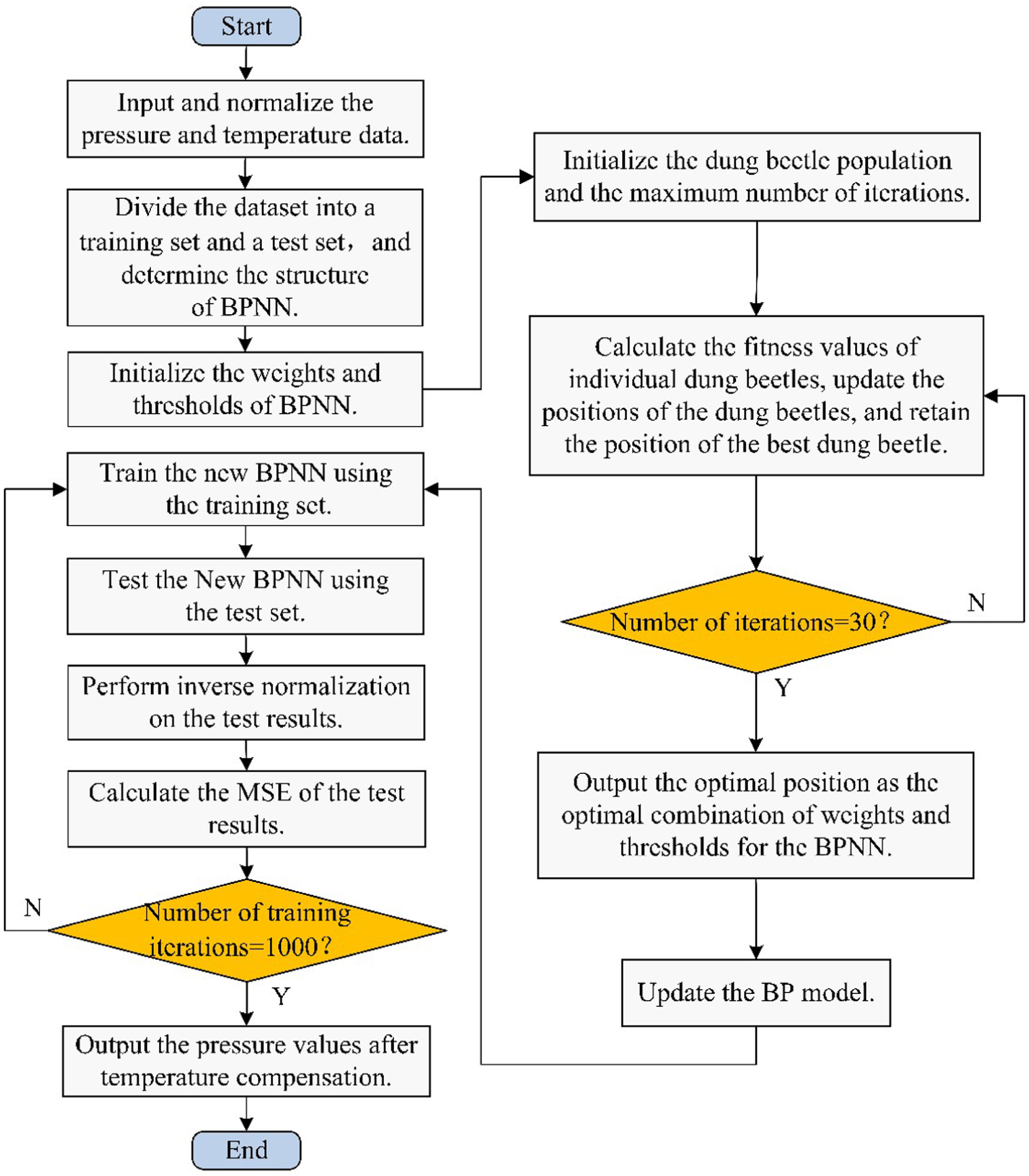
Flowchart of MSDBO-BP algorithm.

Experimental study and result analysis

The MSDBO-BP temperature compensation algorithm is implemented through a hardware system. First, based on the optimized BP neural network weights and thresholds derived from Figures 9 and 10, the FPU unit of the STM32F407VET6 chip is enabled in the MDK compilation environment. DSP library files and related header files are added, and a forward propagation program for the BP neural network is written. Second, the temperature and pressure values at the site are collected in real-time using the temperature-pressure integrated sensor designed in this paper. After filtering, amplification, and sampling hold circuits, the data is input into the STM32F407VET6 microcontroller. After conversion by the internal high-precision ADC, the MSDBO-BP algorithm is executed for intelligent compensation. Finally, the compensated pressure values are output in real-time via RS485. The hardware architecture of this system is shown in Figure 11.

Figure 11.

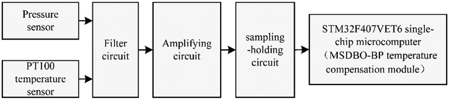
System hardware architecture.

Calibration experiment

The sensor used in the experiment is a temperature-pressure integrated sensor designed for this paper, consisting of a PT100 temperature sensor and a CYX19–32 series oil-filled core from Tianshui Huatian. The sensor operates on a power supply of 15–28 VDC, has a measurement range of 0–50 MPa and can function stably within a wide temperature range of −20°C to 70°C. The experimental setup includes a RIGOL power supply, a host computer, a Druck PACE6000 modular pressure controller with an accuracy of 0.02% FS, and an ESPEC high-temperature and low-temperature test chamber, which simulate industrial site pressure and temperature changes, respectively. The experimental equipment connections are shown in Figure 12.

Figure 12.

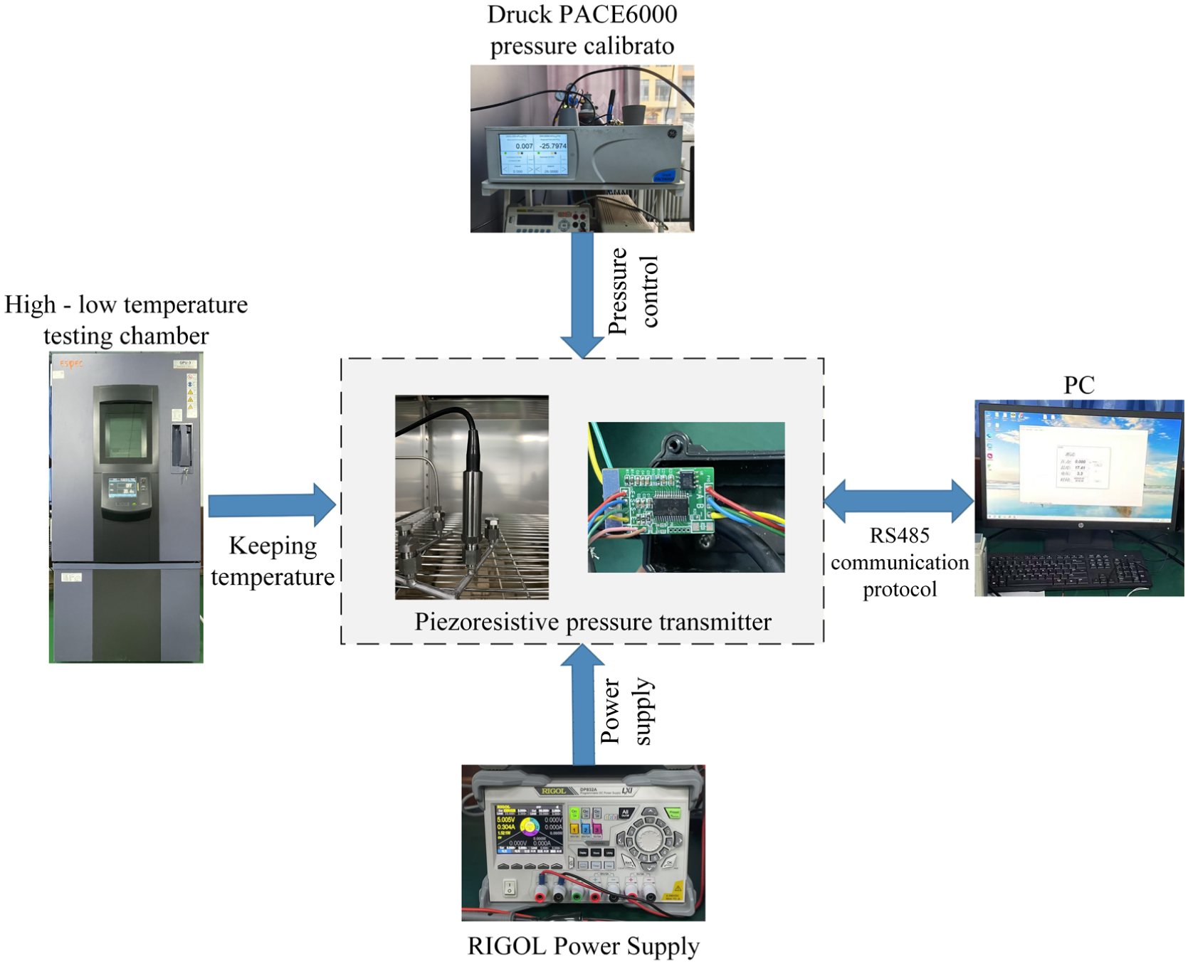
Experimental platform of calibration experiment.

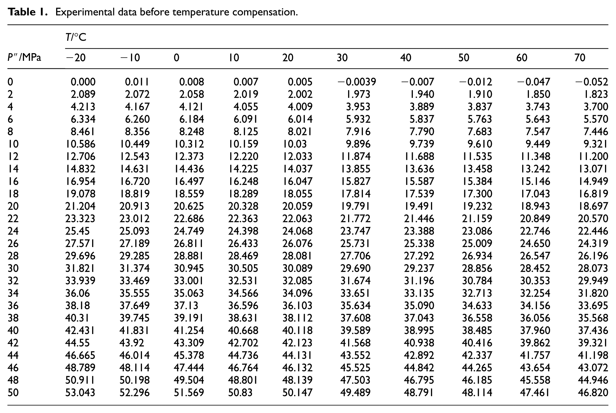
The testing process starts at −20°C, with each temperature point increasing by 10°C, and each temperature point is maintained for 2 h until the temperature reaches 70°C. To avoid hysteresis errors, within the 0–50 MPa range, the pressure is adjusted from low to high in the same direction, with one pressure calibration point selected every 2 MPa, totaling 26 pressure values. The experimental data consists of 260 input-output pairs, as shown in Table 1.

Table 1.

Experimental data before temperature compensation.

P″/MPa	T/°C
	−20	−10	0	10	20	30	40	50	60	70
0	0.000	0.011	0.008	0.007	0.005	−0.0039	−0.007	−0.012	−0.047	−0.052
2	2.089	2.072	2.058	2.019	2.002	1.973	1.940	1.910	1.850	1.823
4	4.213	4.167	4.121	4.055	4.009	3.953	3.889	3.837	3.743	3.700
6	6.334	6.260	6.184	6.091	6.014	5.932	5.837	5.763	5.643	5.570
8	8.461	8.356	8.248	8.125	8.021	7.916	7.790	7.683	7.547	7.446
10	10.586	10.449	10.312	10.159	10.03	9.896	9.739	9.610	9.449	9.321
12	12.706	12.543	12.373	12.220	12.033	11.874	11.688	11.535	11.348	11.200
14	14.832	14.631	14.436	14.225	14.037	13.855	13.636	13.458	13.242	13.071
16	16.954	16.720	16.497	16.248	16.047	15.827	15.587	15.384	15.146	14.949
18	19.078	18.819	18.559	18.289	18.055	17.814	17.539	17.300	17.043	16.819
20	21.204	20.913	20.625	20.328	20.059	19.791	19.491	19.232	18.943	18.697
22	23.323	23.012	22.686	22.363	22.063	21.772	21.446	21.159	20.849	20.570
24	25.45	25.093	24.749	24.398	24.068	23.747	23.388	23.086	22.746	22.446
26	27.571	27.189	26.811	26.433	26.076	25.731	25.338	25.009	24.650	24.319
28	29.696	29.285	28.881	28.469	28.081	27.706	27.292	26.934	26.547	26.196
30	31.821	31.374	30.945	30.505	30.089	29.690	29.237	28.856	28.452	28.073
32	33.939	33.469	33.001	32.531	32.085	31.674	31.196	30.784	30.353	29.949
34	36.06	35.555	35.063	34.566	34.096	33.651	33.135	32.713	32.254	31.820
36	38.18	37.649	37.13	36.596	36.103	35.634	35.090	34.633	34.156	33.695
38	40.31	39.745	39.191	38.631	38.112	37.608	37.043	36.558	36.056	35.568
40	42.431	41.831	41.254	40.668	40.118	39.589	38.995	38.485	37.960	37.436
42	44.55	43.92	43.309	42.702	42.123	41.568	40.938	40.416	39.862	39.321
44	46.665	46.014	45.378	44.736	44.131	43.552	42.892	42.337	41.757	41.198
46	48.789	48.114	47.444	46.764	46.132	45.525	44.842	44.265	43.654	43.072
48	50.911	50.198	49.504	48.801	48.139	47.503	46.795	46.185	45.558	44.946
50	53.043	52.296	51.569	50.83	50.147	49.489	48.791	48.114	47.461	46.820

The characteristic curves of the piezoresistive pressure sensor before temperature compensation can be plotted based on the experimental data obtained at different temperatures and pressures, as shown in Figure 13.

Figure 13.

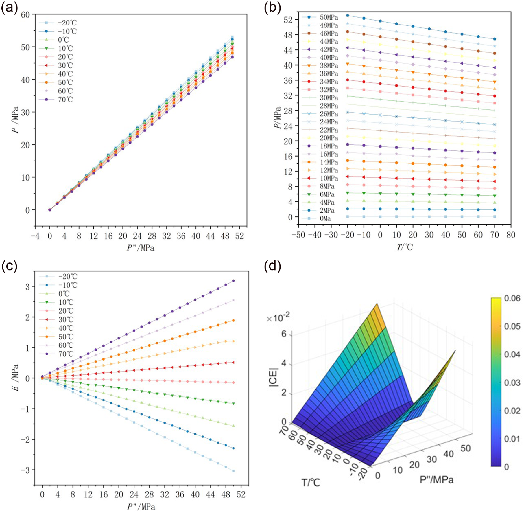
Characteristic curves and graphs of the piezoresistive pressure sensor before temperature compensation: (a) pressure characteristic curve, (b) temperature characteristic curve, (c) output relative error characteristic, and (d) quoted error surface.

To quantitatively evaluate the influence of temperature variation on pressure sensors, this paper introduces the indicators of zero drift coefficient α₀, sensitivity drift coefficient ${\alpha }_{\mathrm{s}}$ , and full-scale accuracy δ. The formulas for calculating these indicators are given in equations ²⁶ :

$${\alpha }_0=\frac{{\left|P_0\right|}_{max}}{P_{\mathrm{FS}}}\times \frac{1}{\mathrm{\Delta }T}$$

(18)

$${\alpha }_{\mathrm{s}}=\frac{|P_{max}-P_{min}|}{P_{\mathrm{FS}}}\times \frac{1}{\mathrm{\Delta }T}$$

(19)

$$\delta =\frac{{\left|\mathrm{\Delta }P\right|}_{max}}{P_{\mathrm{FS}}}\times 100\%$$

(20)

where |P₀|_max is the maximum absolute change of zero pressure within the temperature variation range, P_FS is the pressure output value at the full scale of the pressure sensor, ΔT is the variation range of the sensor’s working temperature, P_max and P_min are respectively the maximum and minimum values of the pressure output obtained under maximum temperature drift conditions, and |ΔP|_max is the maximum absolute error between the output pressure and the standard pressure.

As seen in Figure 13(a), the input-output curves of the sensor at different temperatures are distributed across a band, rather than overlapping, indicating that pressure is influenced by temperature variations. From Figure 13(b), it can be observed that the output value of the pressure sensor, obtained at different pressure points, drifts downward as temperature increases. This drift is most pronounced at 50 MPa, where the slope is the largest. In addition, Figure 13(c) shows that the maximum relative error in the output of the piezoresistive pressure sensor is as large as 3.33 MPa when compared to the reference temperature of 20°C. According to Table 1, P_FS is 50 MPa, ΔT is 90°C, and |P₀|_max is 0.052 MPa. The largest temperature drift occurs when the sensor is subjected to a pressure of 50 MPa. The output pressure P_max is the largest when the temperature is −20°C (which is 53.04 MPa), and the output pressure P_min is the lowest when the temperature is 70°C (which is 46.82 MPa). By substituting these values into equations and for calculation, the zero drift coefficient α ₀  = 1.15 ×10⁻⁵ and sensitivity drift coefficient α _s  = 1.38 ×10⁻³ can be obtained. It can be concluded that significant temperature drift is observed in this piezoresistive pressure sensor. When T is 70°C and P is 50 MPa, the pressure sensor has a maximum absolute error |ΔP|_max of 3.18 MPa. The full-scale accuracyδ = 6.36%, calculated using equation, indicates that temperature drift seriously affects the measurement accuracy of the piezoresistive pressure sensor.

Analysis of temperature compensation results obtained from the MSDBO-BP model

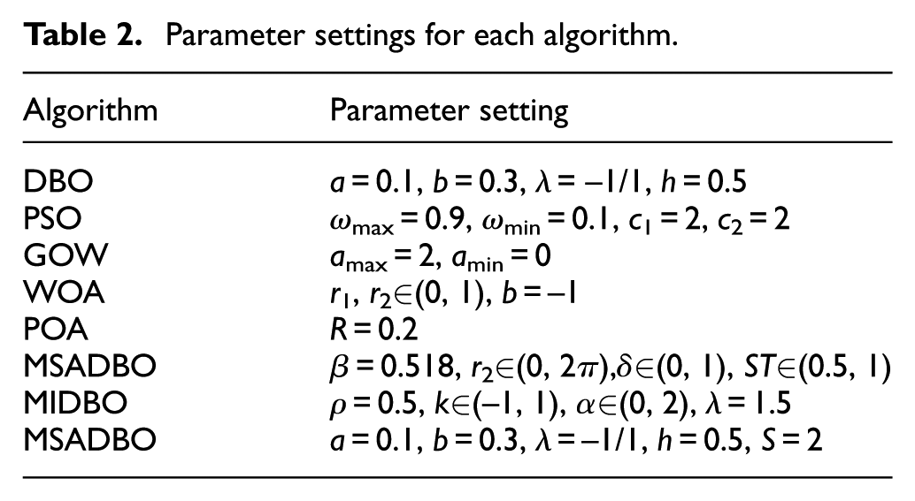
To verify the effectiveness of the MSDBO-BP presented in this study, its compensation performance was compared with that of the traditional BP temperature compensation model, five different meta-heuristic algorithms including the Dung Beetle Optimizer (DBO), Particle Swarm Optimization (PSO), ²⁷ Gray Wolf Optimizer Algorithm (GWO), ²⁸ Whale Optimization Algorithm (WOA), ²⁹ and Pelican Optimization Algorithm, ³⁰ and the BP temperature compensation models based on two improved dung beetle optimization algorithms (MSADBO and MIDBO) proposed by other scholars.^31,32 The above eight models are referred to as BP, DBO-BP, PSO-BP, GWO-BP, WOA-BP, POA-BP, MSADBO-BP, and MIDBO-BP, respectively. The parameter settings for each algorithm are provided in Table 2, with a population size of N = 30 and a maximum iteration count of M = 30. The fitness function of each algorithm is MSE, which quantifies the difference between the standard pressure P″ and the post-compensation pressure P′.

Table 2.

Parameter settings for each algorithm.

Algorithm	Parameter setting
DBO	a = 0.1, b = 0.3, λ = −1/1, h = 0.5
PSO	ωmax = 0.9, ωmin = 0.1, c1 = 2, c2 = 2
GOW	a max = 2, amin = 0
WOA	r 1, r2∈(0, 1), b = –1
POA	R = 0.2
MSADBO	β = 0.518, r2∈(0, 2π),δ∈(0, 1), ST∈(0.5, 1)
MIDBO	ρ = 0.5, k∈(–1, 1), α∈(0, 2), λ = 1.5
MSADBO	a = 0.1, b = 0.3, λ = –1/1, h = 0.5, S = 2

Each algorithm was trained 20 times on the training set, and a fitness curve was randomly selected as shown in Figure 14. It can be observed that MSDBO exhibits the best optimization ability and fastest convergence.

Figure 14.

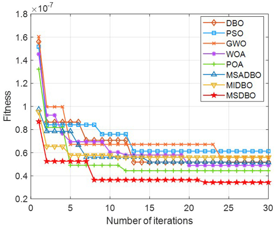
Iteration curves of different algorithms.

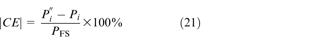
Each model’s efficacy was evaluated via MSE, root mean square error RMSE, mean absolute error MAE, maximum error E_max, minimum error E_min, and absolute quoted error |CE|, the calculation of the quoted error is shown in Equation. ³³ The deviation between the model-predicted pressure values and the calibrated pressure values is measured by MSE and MAE. MAE quantifies the mean absolute deviation of pressure predictions from standard pressures, and |CE| is used to evaluate the performance of the sensor. Tables 3 and 4 detail the algorithm compensation outcomes from training and testing data. The performance comparison of different models on the test set is shown in Figure 15.

$$\left|CE\right|=\frac{{P″}_i-P_i}{P_{\mathrm{FS}}}\times 100\%$$

(21)

Table 3.

Compensation results of each algorithm on the training set.

Algorithm	MSE	RMSE	MAE	E max	E min
BP	1.01E–03	3.19E–02	2.32E–02	2.07E–01		1.40E–04
DBO-BP	1.34E–04	1.16E–02	8.57E–03	3.79E–02		2.25E–05
PSO-BP	1.43E–04	1.20E–02	8.71E–03	3.53E–02		1.89E–04
GWO-BP	1.23E–04	1.11E–02	8.02E–03	3.89E–02		5.50E–05
WOA-BP	9.74E–05	9.87E–03	7.20E–03	3.48E–02		5.68E–07
POA-BP	1.24E–04	1.11E–02	7.92E–03	3.49E–02		7.27E–05
MSADBO-BP	1.36E–04	1.16E–02	8.80E–03	4.46E–02		8.54E–05
MIDBO-BP	1.18E–04	1.08E–02	7.91E–03	3.58E–02		1.54E–04
MSDBO-BP	2.37E–05	4.87E–03	2.46E–03	2.01E–02		5.01E–05

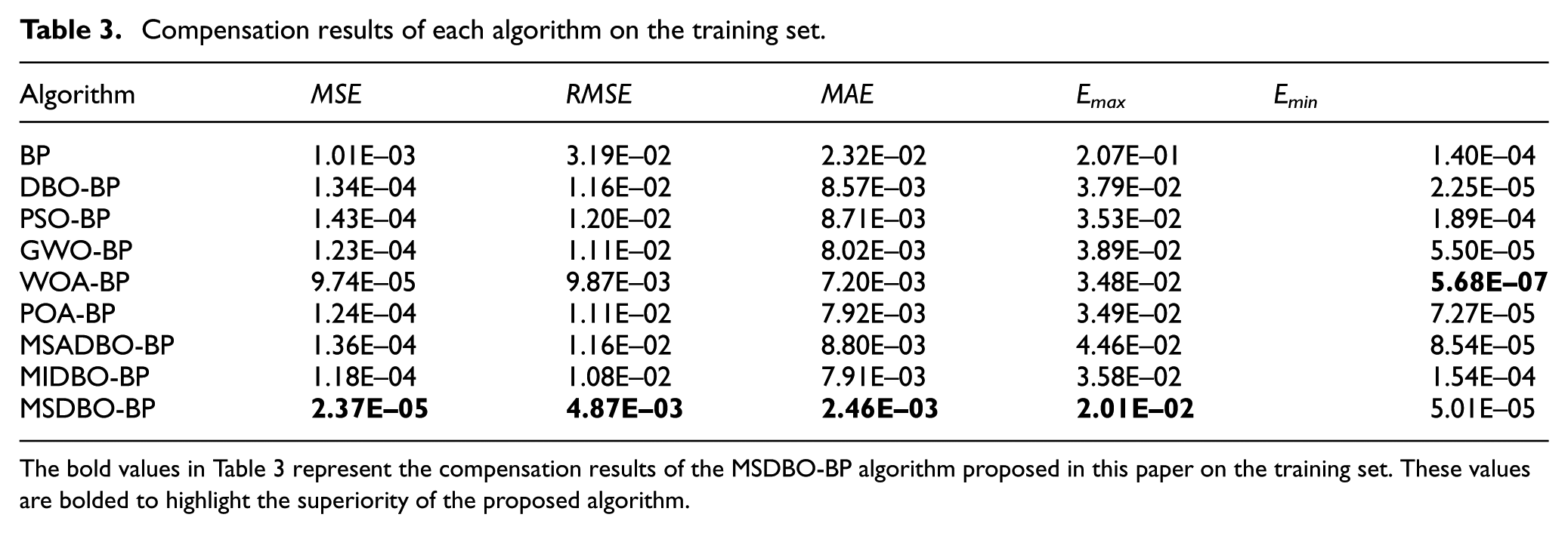
The bold values in Table 3 represent the compensation results of the MSDBO-BP algorithm proposed in this paper on the training set. These values are bolded to highlight the superiority of the proposed algorithm.

Table 4.

Compensation results of each algorithm on the test set.

Algorithm	MSE	RMSE	MAE	E max	E min
BP	1.05E–03	3.24E–02	2.47E–02	9.78E–02	8.08E–05
DBO-BP	1.25E–04	1.12E–02	8.52E–03	2.99E–02	1.21E–04
PSO-BP	7.05E–04	2.66E–02	2.01E–02	8.11E–02	3.69E–04
GWO-BP	1.36E–04	1.17E–02	8.62E–03	3.65E–02	1.99E–04
WOA-BP	1.86E–04	1.36E–02	9.29E–03	3.97E–02	9.92E–06
POA-BP	1.25E–04	1.12E–02	8.64E–03	2.50E–02	1.02E–04
MSADBO-BP	1.99E–04	1.41E–02	1.06E–02	4.10E–02	2.78E–04
MIDBO-BP	1.56E–04	1.25E–02	9.25E–03	3.41E–02	2.33E–04
MSDBO-BP	4.17E–05	6.46E–03	3.46E–03	1.71E–02	4.84E–06

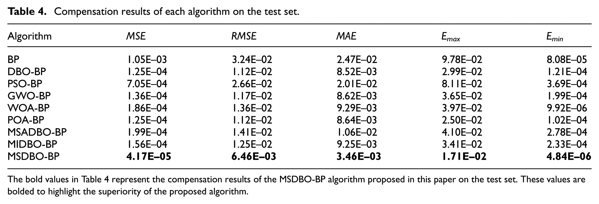
The bold values in Table 4 represent the compensation results of the MSDBO-BP algorithm proposed in this paper on the test set. These values are bolded to highlight the superiority of the proposed algorithm.

Figure 15.

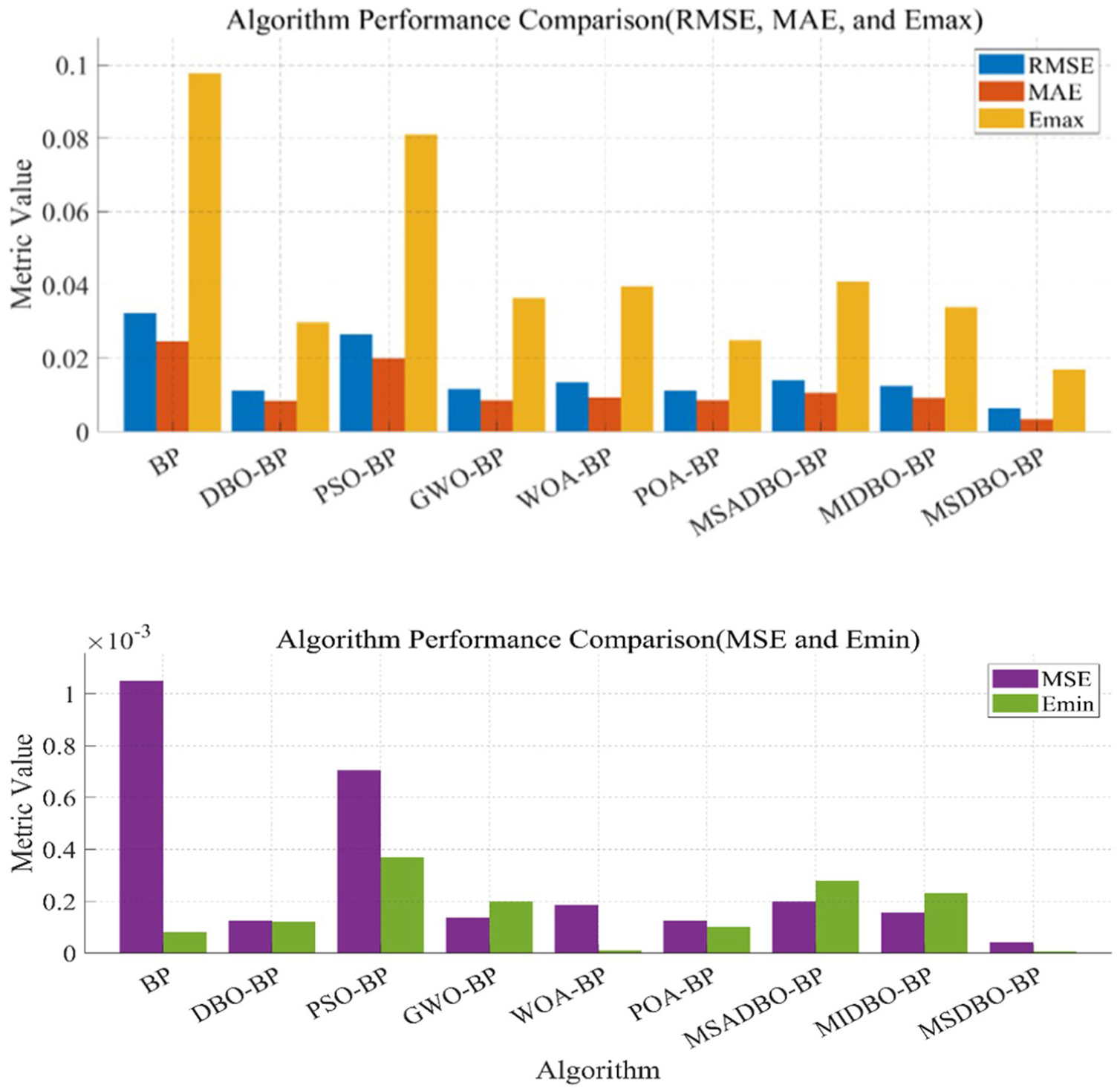
Algorithm performance comparison (test set).

As shown in Tables 3 and 4, the proposed MSDBO-BP model outperforms the other eight models: The post-compensation values of MSE, RMSE, MAE and E_max obtained on the training and test sets are the lowest compared with those of other models, the average error MAE is 2.96 × 10^–3 MPa, and the maximum error E_max is only 2.01 × 10⁻² MPa, indicating excellent compensation performance.

The calculated values of the mean quoted error |CE|_ave, maximum quoted error |CE|_max, and minimum quoted error |CE|_min of the evaluated algorithms are shown in Table 5 with corresponding quoted error surfaces in Figure 16.

Table 5.

Quoted errors of the entire dataset after compensation.

Algorithm	|CE|ave	|CE|max	|CE|min
BP	4.70E–04	4.15E–03	1.62E–06
DBO-BP	1.71E–04	7.59E–04	4.49E–07
PSO-BP	2.20E–04	1.62E–03	3.78E–06
GWO-BP	1.63E–04	7.79E–04	1.10E–06
WOA-BP	1.52E–04	7.94E–04	1.14E–08
POA-BP	1.61E–04	6.99E–04	1.45E–06
MSADBO-BP	1.71E–04	7.66E–04	6.18E–07
MIDBO-BP	1.64E–04	7.16E–04	3.08E–06
MSDBO-BP	7.64E–05	4.17E–04	9.69E–08

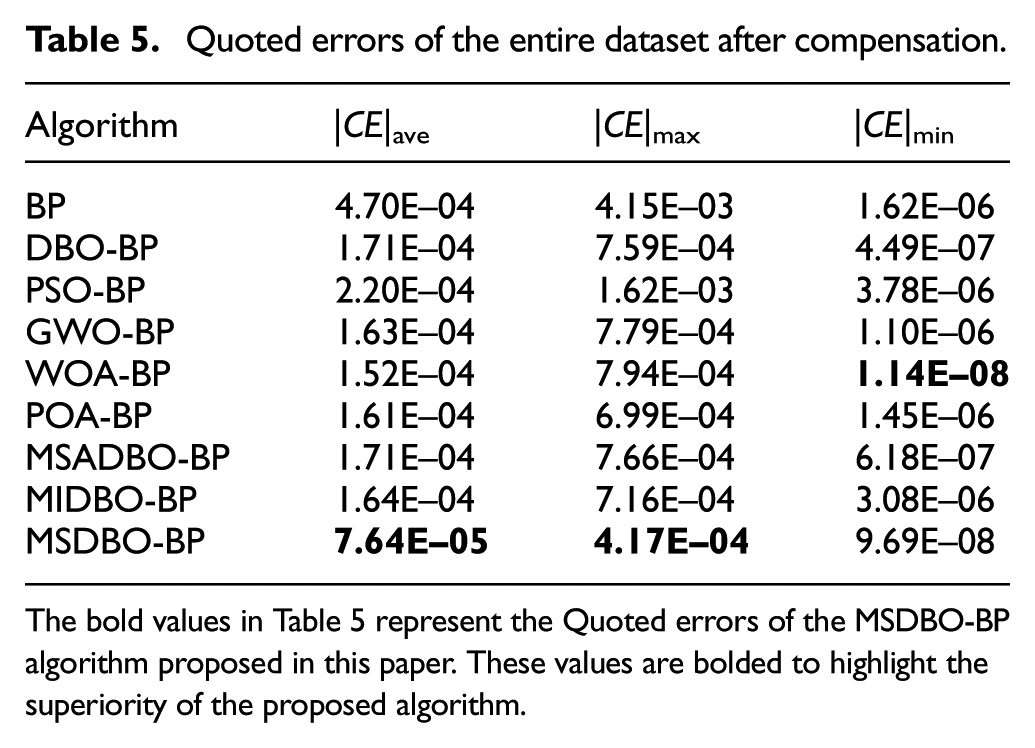
The bold values in Table 5 represent the Quoted errors of the MSDBO-BP algorithm proposed in this paper. These values are bolded to highlight the superiority of the proposed algorithm.

Figure 16.

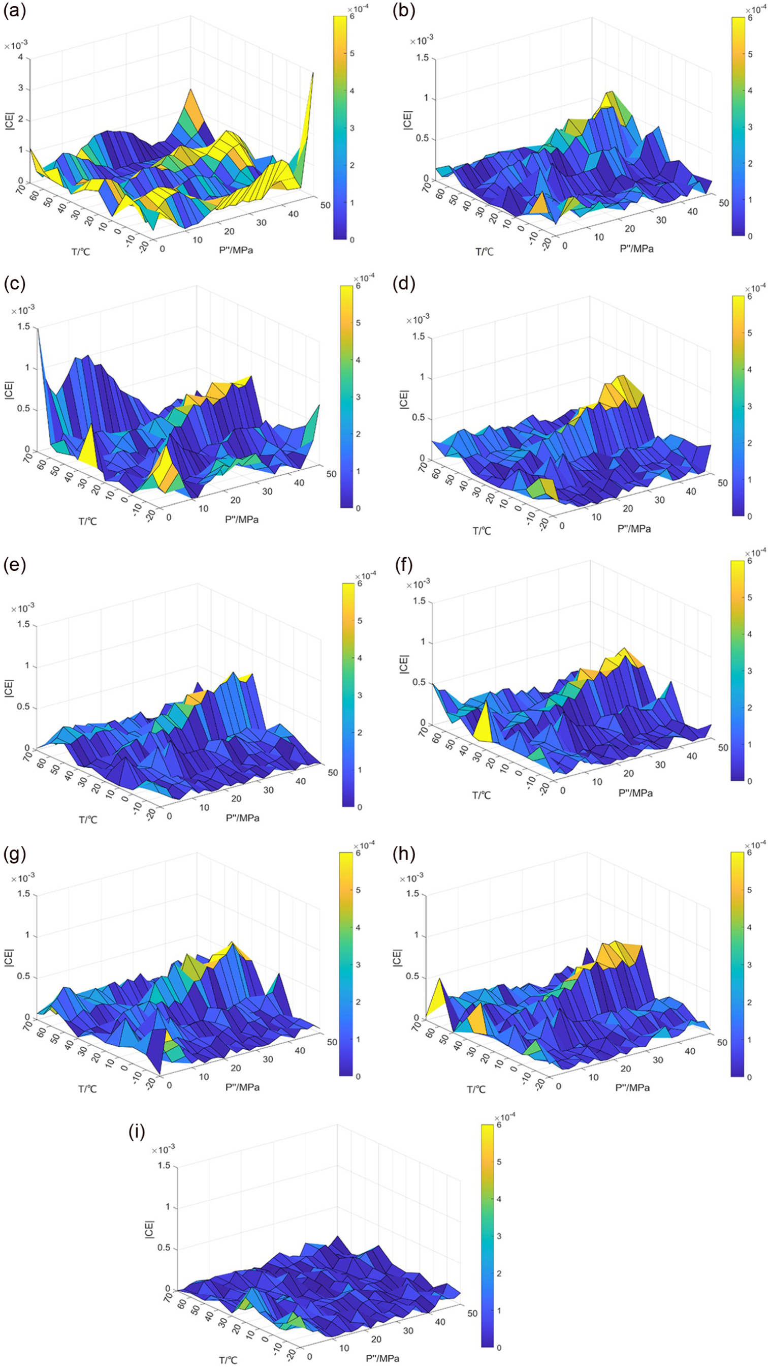
Quoted error surfaces of pressure resistive sensor obtained under the temperature compensation of different temperature compensation models: (a) BP, (b) DBO-BP, (c) PSO-BP, (d) GWO-BP, (e) WOA-BP, (f) POA-BP, (g) MSADBO-BP, (h) MIDBO-BP, and (i) MSDBO-BP.

As seen in Table 5 and Figure 16, the piezoresistive pressure sensor yields a mean quoted error |CE|_ave of 0.076% and a maximum quoted error |CE|_max of 0.42% when the proposed MSDBO-BP model is used to provide temperature compensation, both of which are lower than those of the eight other models. In addition, the quoted error surface yielded by MSDBO-BP is flatter than those of other models, especially in high temperatures of 60°C–70°C, indicating that the compensation accuracy of MSDBO-BP is significantly better than those of other algorithms.

As shown in Figure 17, the pressure-temperature characteristic curves of the piezoresistive pressure sensor used in this experiment significantly improve after compensation by the proposed MSDBO-BP model. A comparison with Figure 13(a) and (b) demonstrates that the model effectively suppresses the negative impact of temperature on the sensor’s output characteristics.

Figure 17.

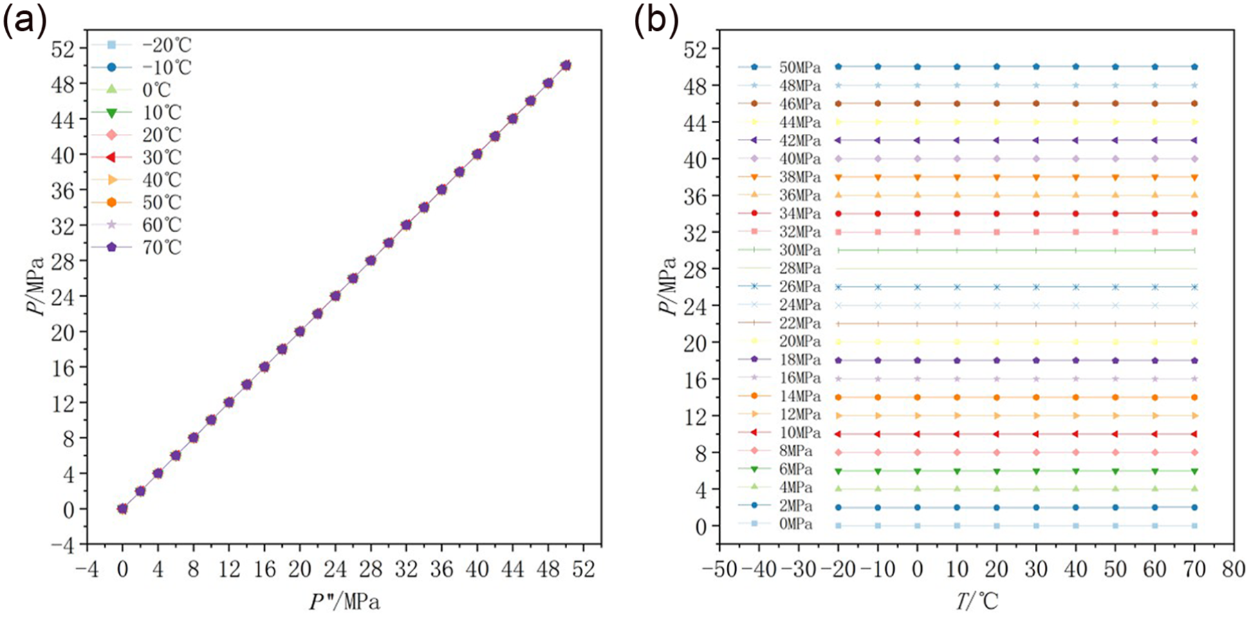
Characteristic curves of piezoresistive pressure sensor under temperature compensation of MSDBO-BP: (a) pressure characteristic curve and (b) temperature characteristic curve.

The calculation results indicate that after temperature compensation, the zero drift coefficient α ₀ and sensitivity drift coefficient α _s are 4.24 × 10⁻⁶ and 4.63 × 10⁻⁶, respectively, representing improvements of one and three orders of magnitude respectively (before temperature compensation, the zero drift coefficient α ₀ and sensitivity drift coefficient α _s are 1.15 × 10⁻⁵ and 1.38 × 10⁻³, respectively), and accuracy δ improves from 6.36% to 0.041%, representing a two-order-of-magnitude increase. A series of experiments demonstrate that the MSDBO-BP compensation model proposed in this paper achieves high compensation accuracy across a large pressure range and a wide temperature range, and it is easily implementable in practical applications. It is particularly noted that the core advantage of the MSDBO-BP model lies in its independence from the structural parameters of specific sensors. Through the nonlinear fitting capability of the BP neural network and the global optimization ability of MSDBO, it adaptively learns the temperature drift characteristics of different sensors, thus possessing excellent versatility for other types of piezoresistive pressure sensors as well as within a wider pressure and temperature range.

Conclusion

• (1) The introduction of the maximin Latin Hypercube sampling method, improved convergence factor, somersault foraging behavior of dung beetles, and adaptive Gaussian-Cauchy perturbation mutation strategy, enhances population diversity, achieves a good balance between global search and local exploration abilities, and solves some problems of the DBO algorithm such as falling into local optima during the optimization process.

• (2) Leveraging MSDBO to fine-tune the weights and thresholds within the BP significantly enhances the temperature compensation model for pressure sensors dealing with a wide pressure and temperature range, boosting both its accuracy and generalization ability. A comparison was made between the model proposed in this paper and eight other temperature compensation models, namely BP, DBO-BP, PSO-BP, GWO-BP, WOA-BP, POA-BP, MSADBO-BP, and MIDBO-BP. The results indicate that the proposed model exhibits more effective compensation. After temperature compensation provided by MSDBO-BP, the zero drift and sensitivity drift coefficients of the sample piezoresistive pressure sensor are reduced by one and three orders of magnitude, respectively, and the full-scale accuracy is improved by two orders of magnitude This indicates that the temperature drift is effectively suppressed, and the measurement accuracy is significantly improved.

• (3) The successful implementation of the proposed temperature compensation model in a piezoresistive pressure sensor transmitter based on STM32F407VET6 and the performance of the model in the following tests demonstrate that the proposed model can reduce hardware compensation cost and improve the measurement accuracy. Future research can further apply artificial intelligence and machine learning to the intelligent temperature compensation of pressure sensors, so as to improve its compensation accuracy and robustness.