Sage Journals: Discover world-class research

Abstract

In complex environments, target acoustic signals are susceptible to interference from background noise during propagation, resulting in the signals captured by sensors being a mixture of valid acoustic emissions and noise. This significantly compromises the accuracy of target localization and damage assessment. To address the nonlinear and non-stationary characteristics of these signals, this paper proposes a novel denoising algorithm termed Improved Variational Mode Decomposition (IVMD)-Wavelet Reconstruction. The core innovation of our method lies in its fully adaptive framework: first, the Singular Value Decomposition (SVD) algorithm is employed to automatically determine the optimal number of intrinsic mode functions (IMFs), K, for the VMD, eliminating a critical manual parameter setting. Second, the correlation coefficient threshold method is utilized to select the optimal IMF components. Subsequently, the noise-dominant components are denoised using a wavelet reconstruction algorithm. Finally, the denoised components and the effective components are reconstructed to achieve the final denoised signal. We have conducted hundreds of experiments, which demonstrate that the proposed algorithm effectively denoises various types of signals and noises, yielding a low Root Mean Square Error (RMSE). Compared to the Ensemble Empirical Mode Decomposition (EEMD) threshold denoising algorithm, the Signal to Noise Ratio (SNR) of the signal processed by our method is increased by 28%, and the Mean Square Error (MSE) is reduced by 52%, which confirming its universality, superiority, and effectiveness.

Keywords

IVMD-wavelet SVD correlation coefficient threshold signal reconstruction processing

Introduction

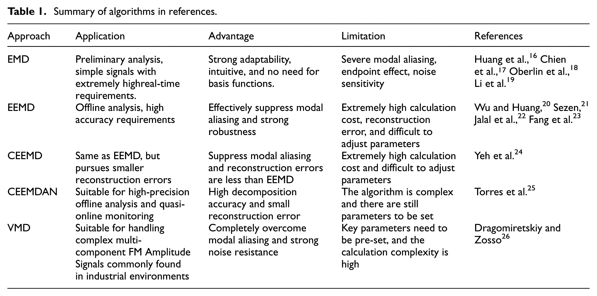
Denoising is an important aspect of signal processing, and denoising quality significantly affects subsequent signal extraction, recognition, analysis, and acoustic positioning.^1–5 Research on denoising methods for nonlinear signals has been a focus of attention in recent years.^6–9 In the system of acoustic sensor array, for each acoustic sensor, interference such as environmental wind or other devices’ noise causes the output signal of the sensor to superimpose many interference components, making signal recognition difficult.^10–15 How to effectively identify acoustic signal information is related to the geometric solution of the acoustic location testing system. In view of the nonlinearity and non-stationarity of the acoustic signals of dynamic objects, empirical mode decomposition (EMD) has advantages in processing the acoustic signals of static objects. However, mode aliasing and end effects are prone to occur during the signal decomposition process. EMD is an algorithm proposed by Huang et al.¹⁶ for detecting signals and decomposing them into the main “patterns.” The algorithm recursively detects the local minimum/maximum value in the signal, estimates the upper and lower envelope by interpolating these extreme values, removes the average value of the envelope as a “low-pass” centerline, thereby isolating the high-frequency oscillations as a “pattern” of the signal, and continues recursively on the remaining “low-pass” centerline. In some cases, this filtering algorithm does indeed decompose the signal into the main mode, however, the final decomposition largely depends on the method of finding the extremum points, the method of interpolating the extremum points into the carrier envelope, and the stopping criteria applied.^17–19 The lack of mathematical theory and the aforementioned degree of freedom reduce the robustness of the algorithm, leaving room for theoretical development and improvement of the robustness of the decomposition. In some experiments, it has been shown that EMD has important similarities with wavelet and (adaptive) filter banks. Ensemble empirical mode decomposition (EEMD) can solve the disadvantages of EMD, but it produces residual white noise when it decomposes the signal.^20–23 CEEMD is an improvement on EEMD. By adding positive and negative white noise in pairs and then averaging, the added white noise residue is almost completely eliminated, and the reconstruction error is smaller than EEMD. However, the calculation cost is extremely high: dozens or even hundreds of EMD decompositions are required, which is very time-consuming, and the application is limited in industrial online monitoring with high real-time requirements, and parameter selection depends on experience.²⁴ CEEMDAN is a further upgrade of CEEMD, with higher completeness and lower reconstruction error. However, the algorithm is more complex and still faces the issue of parameter selection.²⁵ The detailed applications, advantages, and disadvantages of these algorithms are presented in Table 1. Variational Mode Decomposition (VMD) is a signal decomposition method proposed by Dragomiretskiy and Zosso,²⁶ which has significant advantages in the analysis and processing of nonlinear and non-stationary signals. This method can effectively avoid the residual white noise produced by EEMD in the process of signal decomposition. However, when VMD decomposes the signal, the number of intrinsic mode function (IMF) K needs to be set in advance, and the value of K affects the decomposition effect of the algorithm. Based on this, we propose an Improved Variational Mode Decomposition (IVMD)-wavelet reconstruction algorithm and apply it to signal denoising. Its innovation lies in: First, IVMD achieves adaptive parameterization of Variational Mode Decomposition (VMD): unlike traditional VMD that relies on empirical K setting, it uses Singular Value Decomposition (SVD) to automatically determine the optimal decomposition layer K based on the intrinsic characteristics of the signal, eliminating under-decomposition or over-decomposition risks.Second, it introduces targeted IMF screening: the correlation coefficient threshold method effectively distinguishes between useful signal-dominated IMFs and noise-dominated IMFs, avoiding blind processing of all components and improving denoising efficiency. Third, it establishes a modular integration mechanism: the organic combination of adaptive decomposition and precise denoising compensates for the shortcomings of single algorithms, achieving both noise suppression and signal integrity preservation.

Table 1.

Summary of algorithms in references.

Approach	Application	Advantage	Limitation	References
EMD	Preliminary analysis, simple signals with extremely highreal-time requirements.	Strong adaptability, intuitive, and no need for basis functions.	Severe modal aliasing, endpoint effect, noise sensitivity	Huang et al.,¹⁶ Chien et al.,¹⁷ Oberlin et al.,¹⁸ Li et al.¹⁹
EEMD	Offline analysis, high accuracy requirements	Effectively suppress modal aliasing and strong robustness	Extremely high calculation cost, reconstruction error, and difficult to adjust parameters	Wu and Huang,²⁰ Sezen,²¹ Jalal et al.,²² Fang et al.²³
CEEMD	Same as EEMD, but pursues smaller reconstruction errors	Suppress modal aliasing and reconstruction errors are less than EEMD	Extremely high calculation cost and difficult to adjust parameters	Yeh et al.²⁴
CEEMDAN	Suitable for high-precision offline analysis and quasi-online monitoring	High decomposition accuracy and small reconstruction error	The algorithm is complex and there are still parameters to be set	Torres et al.²⁵
VMD	Suitable for handling complex multi-component FM Amplitude Signals commonly found in industrial environments	Completely overcome modal aliasing and strong noise resistance	Key parameters need to be pre-set, and the calculation complexity is high	Dragomiretskiy and Zosso²⁶

Signal denoising method based onIVMD-wavelet transform algorithm

The IVMD model of complex environmental acoustic signals

IVMD is an adaptive signal decomposition algorithm optimized based on the original VMD framework. It addresses the key limitation of VMD, which needs to predefine the number of intrinsic mode functions (IMF) K, by integrating SVD for adaptive K determination and correlation coefficient thresholding for IMF component screening, thereby achieving end-to-end adaptive decomposition and denoising without manual parameter intervention. Assuming that the output of the acoustic sensor contains target acoustic signal and noise signal represented as x(t), and the signal x(t) can be decomposed into k IMF components, then the k-th modal component IMF can be represented as:

u_{k} (t) = A_{k} (t) \cos [ϕ_{k} (t)]

(1)

In (1), $A_{k} (t)$ is the envelope of the signal, which is the instantaneous amplitude of the signal; $ϕ_{k} (t)$ is the phase of the $u_{k} (t)$ signal.

Firstly, the algorithm performs a Hilbert transform on the signal x(t) to obtain the analytic signal of each IMF, which is expressed as

f_{k} (t) = (δ (t) + \frac{j}{π t}) * u_{k} (t)

(2)

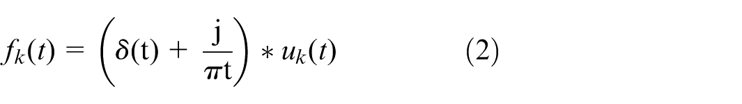
In (2), $f_{k} (t)$ is the decomposed signal for each mode; $δ (t)$ is the Dirac distribution function.

Secondly, the exponential form of the estimated center frequency ω_k is multiplied by equation (2) to obtain the bandwidth of the modal function, which is converted from the spectrum to the baseband.

F_{k} (t) = f_{k} (t) e^{- j ω_{k} t} = [(δ (t) + \frac{j}{π t}) * u_{k} (t)] e^{- j ω_{k} t}

(3)

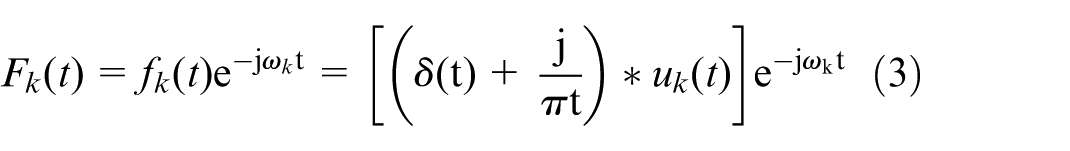
Finally, the algorithm takes the partial derivative of equation (3), then calculates the square of its L2 norm to obtain the bandwidth of each IMF component. The variational model is:

\min_{{u_{k}}, {ω_{k}}} {\sum_{k = 1}^{K} ‖ \partial_{t} [(δ (t) + \frac{j}{π t}) * u_{k} (t)] e^{- j ω_{k} t} ‖_{2}^{2}}

(4)

s . t . \sum_{k = 1}^{K} u_{k} (t) = x (t)

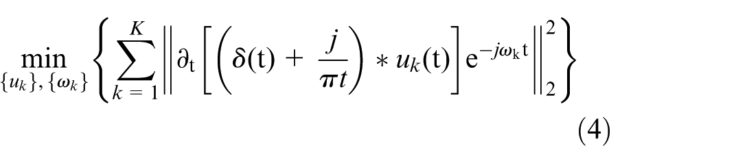
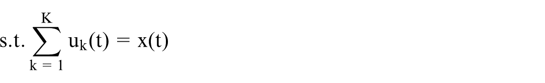
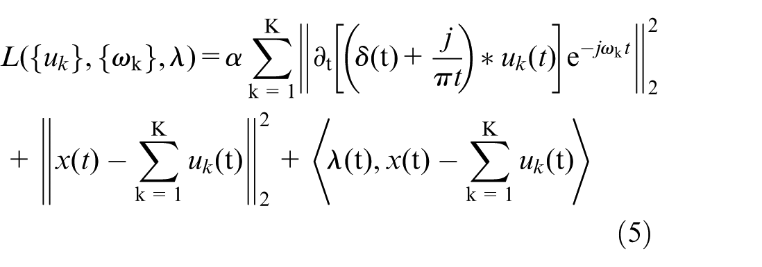
In (4), * represents convolution; $ω_{k}$ is the center frequency of each IMF component.

To solve the variational model in equation (4), the augmented Lagrangian function is constructed by introducing the Lagrange multiplier λ(t) and the quadratic penalty term, which converts the constrained optimization problem into an unconstrained one, facilitating iterative solution via the Alternating Direction Method of Multipliers (ADMM). The expression of the augmented Lagrangian function is

\begin{array}{l} L ({u_{k}}, {ω_{k}}, λ) = α \sum_{k = 1}^{K} {‖ \partial_{t} [(δ (t) + \frac{j}{π t}) * u_{k} (t)] e^{- j ω_{k} t} ‖}_{2}^{2} \\ + {‖ x (t) - \sum_{k = 1}^{K} u_{k} (t) ‖}_{2}^{2} + 〈 λ (t), x (t) - \sum_{k = 1}^{K} u_{k} (t) 〉 \end{array}

(5)

According to alternate direction method of multipliers algorithm (ADMM), $u_{k}^{n + 1}$ , $ω_{k}^{n + 1}$ , $λ_{k}^{n + 1}$ are iteratively updated to obtain the “saddle point” of augmented Lagrange expression.

{\hat{u}}_{k}^{n + 1} (ω) = \underset{{\hat{u}}_{k}, u_{k} \in X}{argmin} {\begin{matrix} α ‖ j ω [1 + sgn (ω + ω_{k})] {\hat{u}}_{k} (ω + ω_{k} ‖_{2}^{2} \\ + ‖ \hat{x} (ω) - \sum_{i} {\hat{u}}_{i} (ω) + \frac{\hat{λ} (ω)}{2} ‖ \end{matrix}}

(6)

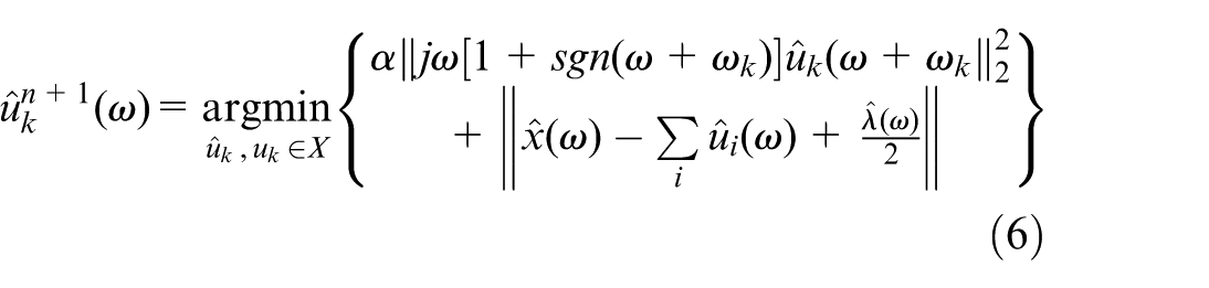
Change the ω variable to $ω - ω_{k}$ , then

\begin{matrix} {\hat{u}}_{k}^{n + 1} (ω) = \underset{{\hat{u}}_{k}, u_{k}}{argmin} \\ {\begin{matrix} α ‖ j (ω - ω_{k}) [1 + sgn (ω + ω_{k})] {\hat{u}}_{k} (ω + ω_{k} ‖_{2}^{2} \\ + ‖ \hat{x} (ω) - \sum_{i} {\hat{u}}_{i} (ω) + \frac{\hat{λ} (ω)}{2} ‖ \end{matrix}} \end{matrix}

(7)

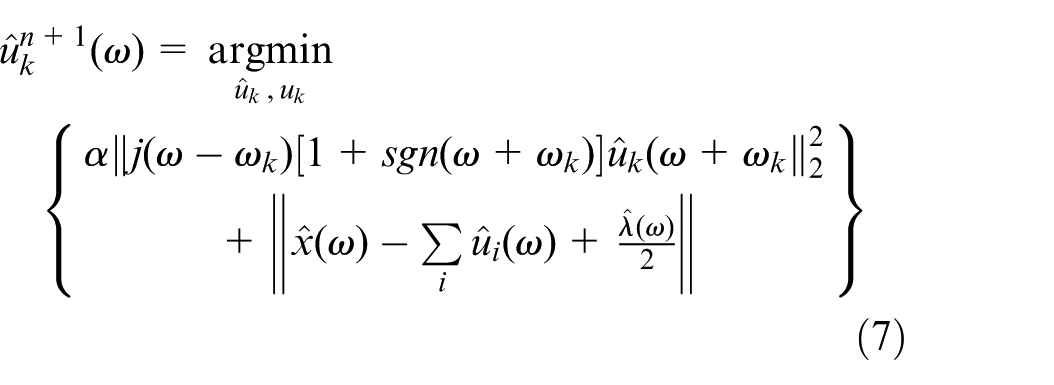
Using the Hermitian symmetry of the real signal in the reconstructed fidelity term, these two terms are written as half-space integrals over non-negative frequencies:

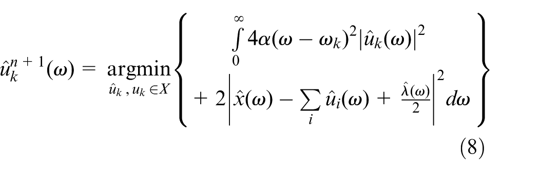
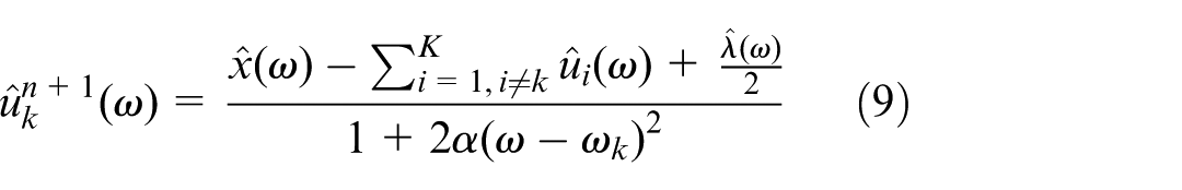
{\hat{u}}_{k}^{n + 1} (ω) = \underset{{\hat{u}}_{k}, u_{k} \in X}{argmin} {\begin{matrix} \int_{0}^{\infty} 4 α {(ω - ω_{k})}^{2} {| {\hat{u}}_{k} (ω) |}^{2} \\ + 2 {| \hat{x} (ω) - \sum_{i} {\hat{u}}_{i} (ω) + \frac{\hat{λ} (ω)}{2} |}^{2} d ω \end{matrix}}

(8)

Then the optimal solution of the quadratic optimization problem is as follows:

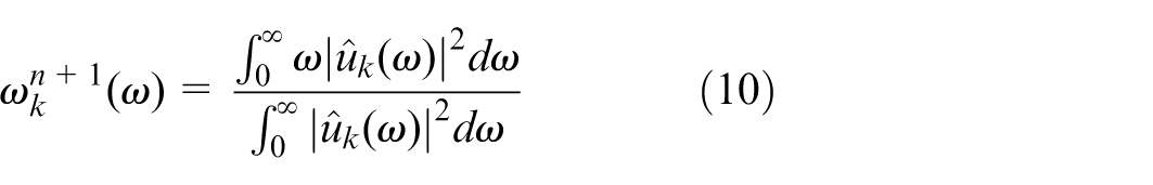
{\hat{u}}_{k}^{n + 1} (ω) = \frac{\hat{x} (ω) - \sum_{i = 1, i \neq k}^{K} {\hat{u}}_{i} (ω) + \frac{\hat{λ} (ω)}{2}}{1 + 2 α {(ω - ω_{k})}^{2}}

(9)

Updated the center frequency, then

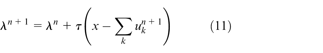
ω_{k}^{n + 1} (ω) = \frac{\int_{0}^{\infty} ω {| {\hat{u}}_{k} (ω) |}^{2} d ω}{\int_{0}^{\infty} {| {\hat{u}}_{k} (ω) |}^{2} d ω}

(10)

Updated the Lagrange multiplier

λ^{n + 1} = λ^{n} + τ (x - \sum_{k} u_{k}^{n + 1})

(11)

Calculation method of modal number based on SVD

When the VMD algorithm is used to decompose the signal, the key is to determine the mode number K. When the K value is less than the number of useful components in the signal, the VMD algorithm fails to decompose the signal sufficiently. When the K value is greater than the number of useful components in the signal, over-decomposition by VMD occurs. Therefore, it is necessary to determine the number of decomposition layers K.

In this paper, we use Singular Value Decomposition (SVD) algorithm to calculate the number of VMD modes. The principle of SVD is to decompose the original signal and obtain a series of singular values through matrix operations. Useful signals are mainly reflected on the first n larger singular values, while noisy signals correspond to smaller singular values. By discarding smaller singular values, noise components can be eliminated, and then the inverse process of SVD can be performed to obtain the denoised signal. The theoretical basis of SVD-based K selection lies in the low-rank characteristic of useful signals. For the constructed Hankel matrix H = R + W, in which R is the useful signal matrix, W is the noise matrix, R has a low-rank structure due to the concentration of dominant frequency components, while W is a random matrix with uniformly distributed singular values. According to the singular value gap theory, the singular values corresponding to R are significantly larger than those of W, and the maximum difference between adjacent singular values indicates the boundary between useful signals and noise, which is the optimal effective rank m (i.e. VMD’s K). The specific implementation method is as follows:

Signal x(t) can be regarded as the superposition of real signal and noise signal, expressed as:

x_{k} = r_{k} + w_{k}

(12)

In (12), is the real target signal, w_k is Gaussian white noise, k = 1,2,…,N; N is the length of the data.

Its Hankel matrix r_k is:

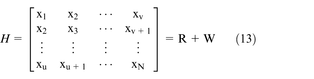
H = [\begin{matrix} x_{1} & x_{2} & \dots & x_{v} \\ x_{2} & x_{3} & \dots & x_{v + 1} \\ ⋮ & ⋮ & ⋮ & ⋮ \\ x_{u} & x_{u + 1} & \dots & x_{N} \end{matrix}] = R + W

(13)

In (13), N = u + v − 1, R is the actual signal matrix, W is the noise signal matrix. The dimensions of the Hankel matrix are set as u = N/2 and v = N − u + 1. This setting balances temporal information retention and computational efficiency, ensuring the matrix retains complete signal characteristics while avoiding excessive computation.

Perform singular value decomposition on H, then

H = P \sum Q^{T} = \sum_{i = 1}^{r} σ_{i} H_{i}

(14)

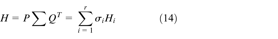
In (14), $P \in R^{u \times u}$ is the left singular matrix, $Q \in R^{v \times v}$ is the right singular matrix, P and Q are orthogonal matrices, $Σ = diag (σ_{1}, σ_{2}, \dots, σ_{r})$ is a diagonal matrix, σ_i is the singular value of H, and r is the rank of the matrix H.

The optimal effective rank, and hence the VMD parameter K, is determined by identifying the index m that corresponds to the maximum relative change between consecutive singular values. This is found by calculating the difference spectrum D(m) = σ_m – σ_m₊₁ for m = 1, 2,…, r – 1. The index m for which D(m) is maximized is selected as the optimal K. This point, K = argmax_mD(m), represents the most substantial drop in energy, effectively separating the signal-dominated components (first K modes) from the noise-dominated ones (remaining modes). This data-driven approach eliminates the need for empirical guesswork and enhances the robustness of the decomposition across different signal and noise types.

Modal component selection based on cross-correlation coefficient

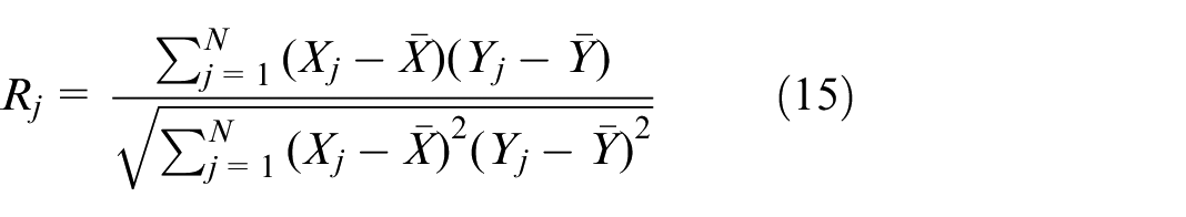
After VMD decomposition, each modal component IMF contains different frequency bands. The noise components with more abnormal signals have lower correlation with the original signal, and the correlation coefficient between the two is relatively small. The correlation between useful signal components and the original signal is better, and the correlation coefficient between the two is relatively larger. Therefore, the correlation coefficient between the original signal and each component signal is chosen as the basis. There is a critical threshold for the correlation coefficient between two components. If the correlation coefficient is higher than the threshold, it is considered that the component contains useful signal components. If the cross-correlation coefficient is below the threshold, it is considered that the component contains noise or abnormal components. The formula for calculating the threshold R_thr is as follows:

R_{j} = \frac{\sum_{j = 1}^{N} (X_{j} - \bar{X}) (Y_{j} - \bar{Y})}{\sqrt{\sum_{j = 1}^{N} {(X_{j} - \bar{X})}^{2} {(Y_{j} - \bar{Y})}^{2}}}

(15)

R_{thr} = \frac{\max (R_{j})}{10 \max (R_{j}) - 3}

(16)

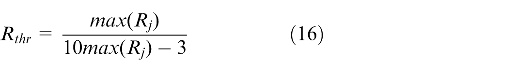
Where, R_j is the correlation coefficient between the j-th IMF component and the original signal; X_j is the original signal, Y_j is the IMF component, $\bar{X}$ and $\bar{Y}$ are the data mean, N is the signal length. If $R_{j} > R_{thr}$ , it is the effective component, and if $R_{j} < R_{thr}$ , it is the noise component.

The threshold formula (16) is empirically derived from extensive testing on various acoustic signals. This formulation adapts the threshold level based on the maximum correlation coefficient observed among the IMFs. A higher max(R_j) indicates a stronger overall signal component presence, thus allowing for a more stringent threshold. This adaptive rule was found to be more effective than a fixed threshold across different signal-to-noise ratio conditions, as it dynamically adjusts to the specific characteristics of the signal under analysis.

Filtering and processing method of complex acoustic signal based on wavelet transform

If the original signal contains the acoustic signal of the target object and the noise signal represented as f(t), then

f (t) = y (t) + s (t)

(17)

In (17), y(t) is the acoustic signal of the target object without noise, s(t) is the noise signal. If wavelet transform is applied to f(t), then:

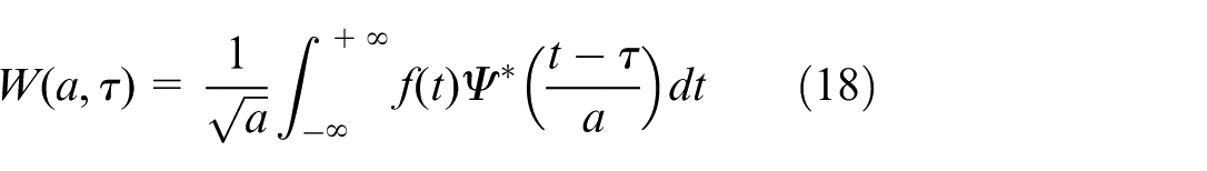
W (a, τ) = \frac{1}{\sqrt{a}} \int_{- \infty}^{+ \infty} f (t) Ψ^{*} (\frac{t - τ}{a}) dt

(18)

In (18), a is the scale factor, τ is the time shift factor, and $Ψ^{*} (\frac{t - τ}{a})$ is the conjugate function of the wavelet generating function $Ψ (t)$ .

The values that change in the frequency domain can be used to perform bandpass filtering on the sound signal. Discretize the signal $f (t)$ and represent it as $f (n)$ . In the algorithm, n represents the discrete sampling points of the acoustic signal. Through orthogonal wavelet decomposition, we obtain the wavelet scale coefficient b_i,j and the wavelet coefficient c_i,j. $b_{i, j} = \sum_{n} h_{1} (2 j - n) b_{i - 1, j}$ , $c_{i, j} = \sum_{n} h_{2} (2 j - n) c_{i - 1, j}$ , $h_{1} (n)$ , and $h_{2} (n)$ are a pair of orthogonal mirror filter banks. $h_{1} (n)$ is the low-pass filter coefficient, which, when applied to the signal, yields a low-frequency smooth profile A_j. $h_{2} (n)$ is the high-pass filter coefficient, which, when applied to the signal, results in a high-frequency detail part B_j. i is the number of wavelet decomposition layers. The wavelet reconstruction function is

e_{j, k} = \sum^{e_{j + 1, n}} h_{1} (j - 2 n) + \sum^{c_{i + 1, n}} h_{2} (j - 2 n)

(19)

Based on the reconstruction function, the Daubechies 5 (db5) wavelet is selected to perform a three-layer decomposition of the acoustic signal, due to its optimal time-frequency localization and high correlation with acoustic signals compared to db2, db3, sym4, and coif3 wavelet. The reason for using three-layer decomposition is the third low-frequency component A3 contains 90% of useful signal energy, while first to third high-frequency components (B1–B3) are dominated by noise. Increasing to four layers increases computation time by 40% without improving denoising effect. In order to eliminate the high-frequency components of the acoustic signal, the wavelet coefficients w_i,j of the acoustic signal are divided into two parts: one is the wavelet coefficient s_i,j representing the sound signal, and the other is the wavelet coefficient n_i,j representing the noise signal, with $w_{i, j} = s_{i, j} + n_{i, j}$ .

The main algorithm for introducing Stein’s Unbiased Risk Estimate (SURE) rule is as follows:

Let W be a vector whose elements are the square W_k of wavelet coefficients $w (i, j)$ arranged in ascending order, and k be the number of wavelet coefficients, resulting in a vector $W = W_{1}, W_{2}, \dots, W_{k}$ that satisfies $W_{1} \leq W_{2} \leq \dots \leq W_{k}$ . Then, construct a risk vector and calculate the minimum risk value. Assuming a risk vector $F = F_{1}, F_{2}, \dots, F_{k}$ , its elements are:

F_{m} = \sum_{l = 1}^{m} W_{l} / k + (k - 2 m) + (k - m) W_{m}

(20)

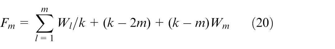
Through iteration, the minimum value F_r is taken as the risk value, and the corresponding W_r is calculated from the subscript r of F_r. Then the threshold δ is calculated, $δ = \sqrt{σ^{2} W_{r}}$ . The soft threshold function is used to obtain the estimated original signal wavelet coefficient $w (i, j)$ to make $w' (i, j)$ as small as possible. Then $w (i, j)$ is used for wavelet reconstruction to obtain the estimated target object’s signal $f' (t)$ after noise removal.

A denoising method for complex acoustic signals based on IVMD-wavelet

The optimal effective rank order obtained from SVD decomposition of signals can determine the number of modes K for VMD decomposition, which not only separates the signal from the noise signal, but also avoids the problem of over decomposition of VMD decomposition signals. After VMD decomposition, the correlation coefficients between the original signal and each component signal are selected as the basis for IMF filtering, forming the IVMD denoising algorithm. Preserve the obtained IMF effective components, perform wavelet reconstruction denoising on the obtained IMF preprocessed components, and then reconstruct them with the IMF effective components to obtain the denoised signal, forming the IVMD-wavelet reconstruction denoising processing algorithm. Figure 1 shows the flow diagram of the IVMD-wavelet denoising algorithm.

Figure 1.

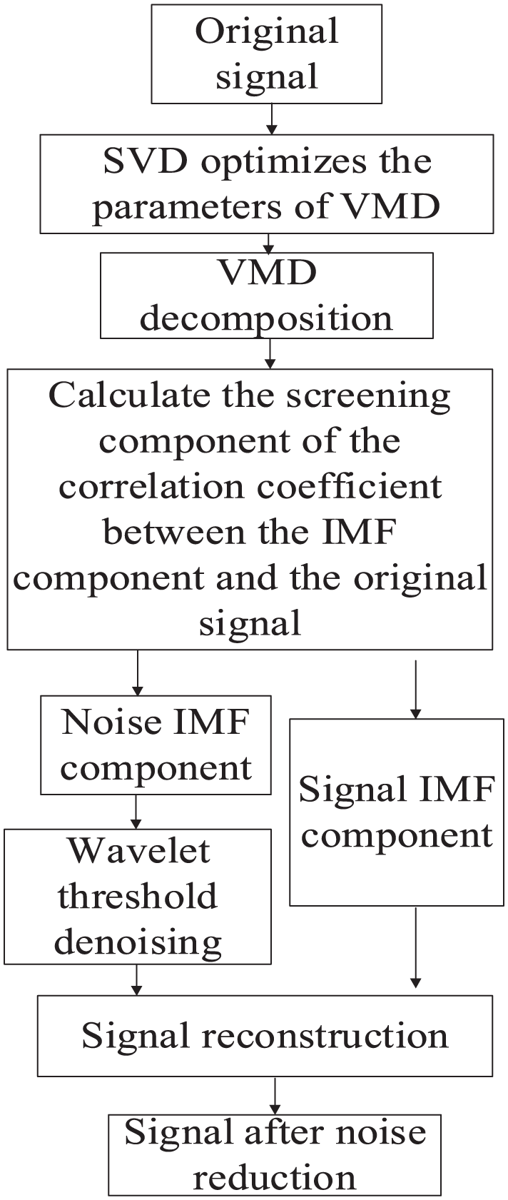
Flow diagram based on IVMD-wavelet denoising algorithm.

The specific algorithm is as follows:

(1) Perform SVD on the acoustic signal of the object collected by the acoustic sensing array.

(2) Calculate the optimal effective rank order k for singular values, which is the k-layer modal decomposition of IVMD.

(3) Use the correlation coefficients between the original signal and each component signal to screen the IMF, extract the effective components and the components to be processed;

(4) Apply db5 wavelet reconstruction denoising to IMF preprocessed components, and use stein’s unbiased likelihood estimation for threshold calculation at each layer;

(5) Reconstruct the obtained effective IMF com-ponents and wavelet thresholded denoised components.

Calculation and experimental analysis

Calculation of the optimal mode number K

In order to calculate the optimal mode number K in the IVMD algorithm, we selected a firecracker’s explosion signal for SVD decomposition. Figure 2 shows the detection of firecracker’s explosion acoustic information using an acoustic sensing array, Figure 3 shows the acoustic signal output by a single sensor, and Figure 4 shows the singular value distribution curve, where m is the order of the singular value, σ is singular value.

Figure 2.

Detecting acoustic signals of target using acoustic sensing arrays.

Figure 3.

Target acoustic signal and speech spectrum.

Figure 4.

Singular value distribution curve.

From Figure 4, it can be observed that the corresponding singular values change abruptly when m = 9 and 12. According to the method for determining the optimal effective rank order of singular values in Section 2.2, it can be determined that when m = 9, it is the optimal effective rank order. Therefore, the number of IMF components for VMD decomposition is determined to be 9.

Screening of IMF components in IVMD

Since the explosion sound signal of firecrackers in a noisy environment detected by the acoustic sensor array device is interfered by white noise, which has an adverse effect on the subsequent calculation of target acoustic location, in this experiment, Gaussian white noise is superimposed on the collected original signal of firecracker explosion, and 10 dB Gaussian white noise is added to the collected explosion sound signal. The waveform of the noisy signal obtained is shown in Figure 5.

Figure 5.

Noisy signal waveform diagram.

Perform IVMD decomposition on the noisy signal, optimize the parameter K = 9, and calculate the correlation between each modal component IMF and the noisy signal, as shown in Figure 6, the correlation coefficient threshold obtained using equation (16) is 0.1499. If the correlation coefficient of IMF1–IMF4 is greater than the threshold, it is an effective component and is retained; If the correlation coefficient of IMF5–IMF9 is less than the threshold, it is the component to be processed, and wavelet threshold denoising is performed.

Figure 6.

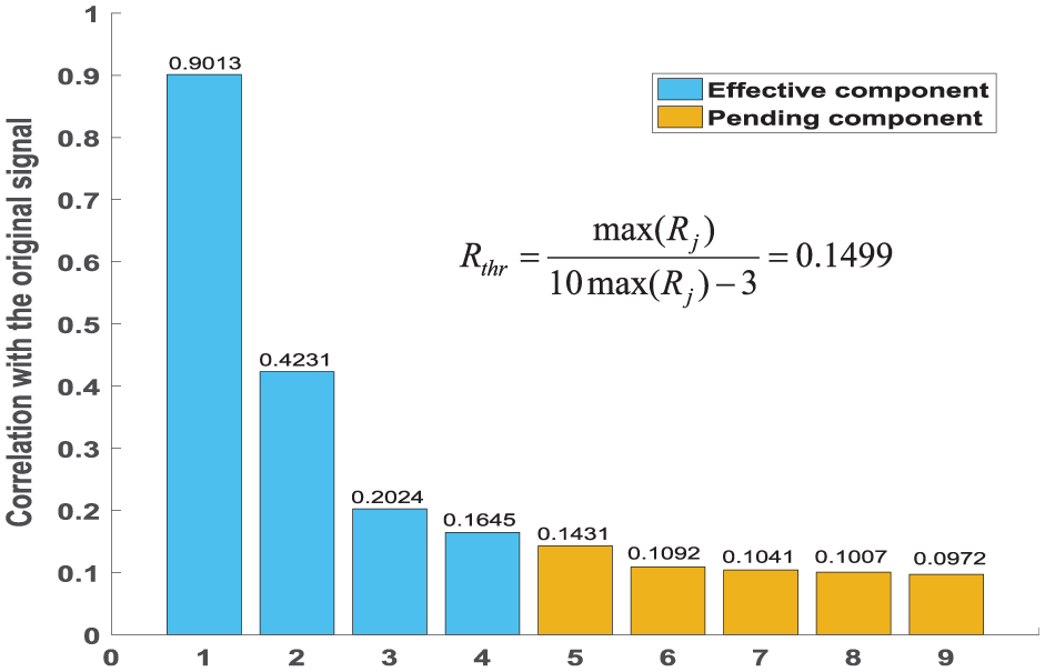
The correlation degree between each IMF component and the noisy signal.

Screening of IMF components in IVMD

In this experiment, the explosion sound signal of firecrackers in a complex environment was collected as the original signal, and 10 dB Gaussian white noise was added to form a noisy signal. db5 was used as the wavelet function for 3-layer decomposition, and stein’s unbiased likelihood estimation principle was used to calculate the threshold of each layer. Finally, the denoising effect of db5 was measured. The specific experimental process is shown in Figure 7 and Figure 8.

Figure 7.

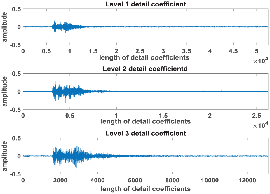
Three-layer decomposition based on db5 wavelet function.

Figure 8.

Comparation of the original signal and the reconstructed signal after denoising with db5.

According to the experimental results, SNR = 11.23 dB and RMSE = 0.3712 after using db5 wavelet threshold denoising. It can be seen that db5 wavelet denoising can effectively filter, and the variance is small, and the method is feasible.

Evaluation of denoising performance of IVMD-wavelet reconstruction algorithm

Experiment 1

Collect the sound signal of firecracker’s explosion as the original signal, in order to more intuitively evaluate the IVMD-wavelet reconstruction filtering algorithm, we add 20 dB Gaussian white noise to the original signal to form the denoised audio signal. The IVMD algorithm is applied to decompose the denoised signal into nine layers, and the correlation coefficient method is used to filter the IMF. The processed components are subjected to wavelet threshold filtering before reconstruction. The process of adding 20 dB signal denoising is shown in Figure 9; Where K = 9, α = 2500. The penalty parameter α in IVMD controls the bandwidth of the IMFs. A value of α = 2500 was selected after a parametric study. This value provides a good trade-off: it is high enough to enforce narrowband modes and suppress noise, but not so high as to cause excessive smoothing and loss of signal details.

Figure 9.

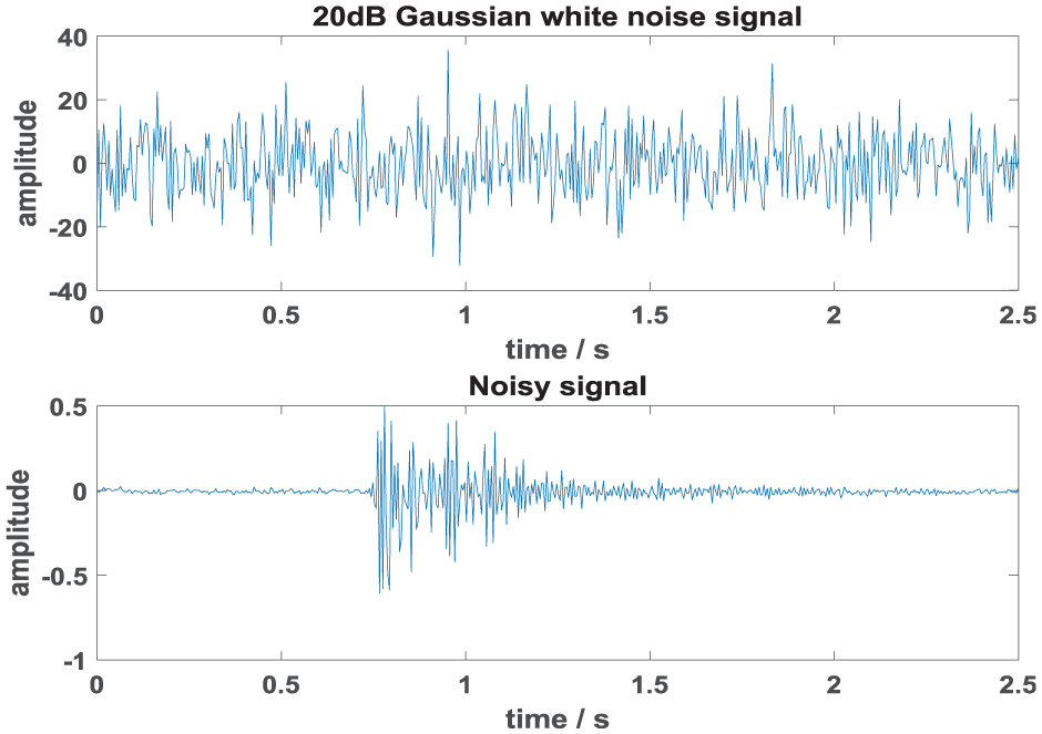
Waveform of the original signal contaminated with additive 20 dB Gaussian white noise.

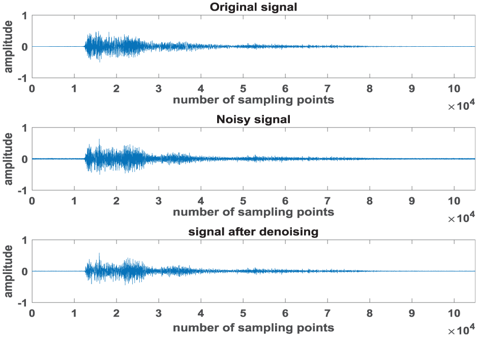
Figure 9 shows the IVMD decomposition of the firecracker explosion signal with 20 dB Gaussian white noise, Figure 10 shows the spectral decomposition diagram of the signal containing 20 dB noise, Figure 11(a) shows the spectral diagrams of each mode, Figure 11(b) shows the original noise signal formed by the superimposed 20 dB noise signal and the 20 dB Gaussian white noise signal, and Figure 12 shows the reconstructed signal obtained after denoising using IVMD-wavelet threshold algorithm. After denoising, SNR = 37.718 dB and RMSE = 0.03043 were calculated.

Figure 10.

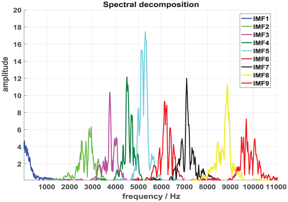
Spectral decomposition diagram of the signal with 20 dB Gaussian white noise.

Figure 11.

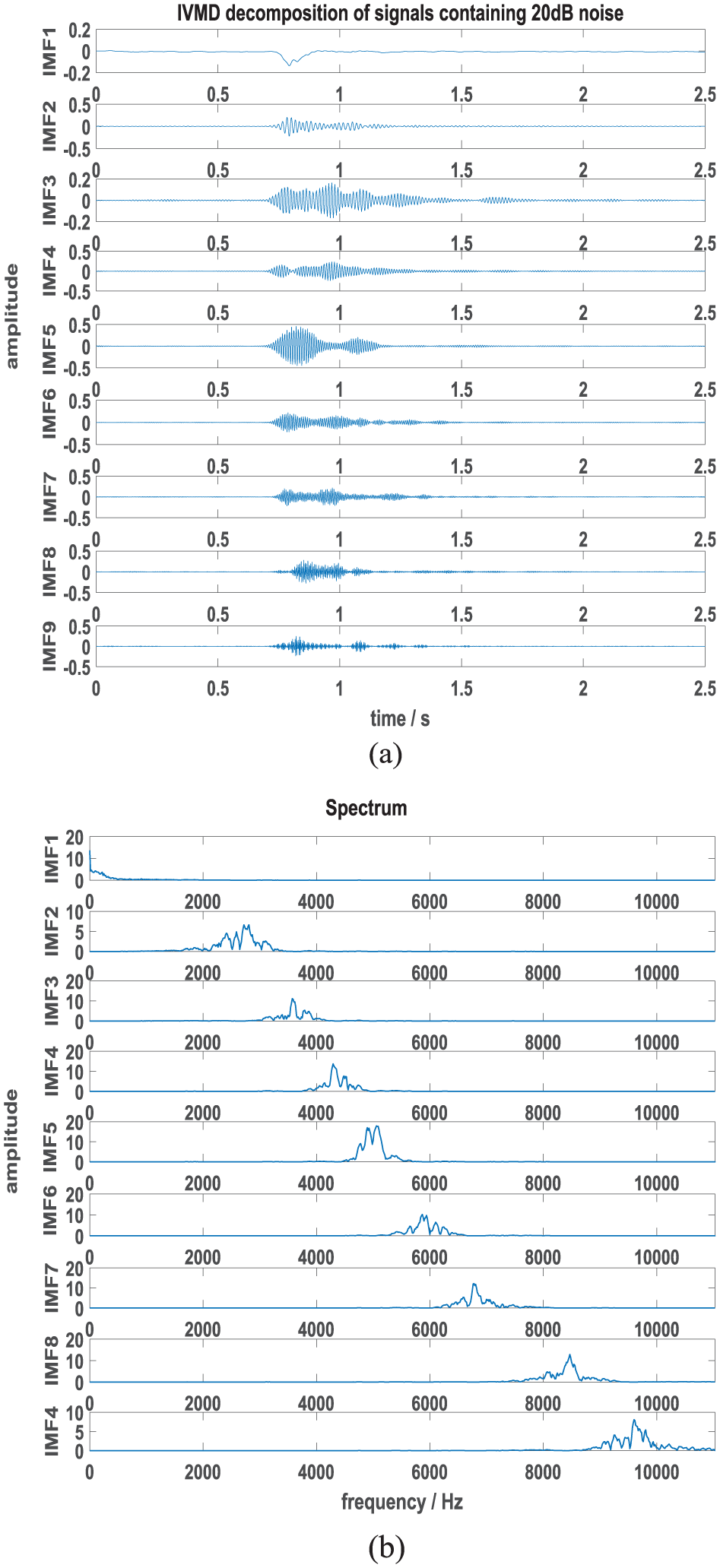
IVMD decomposition and its modal spectrum diagram: (a) IVMD decomposition of 20 dB noisy signal and(b) spectrum of each IMF component.

Figure 12.

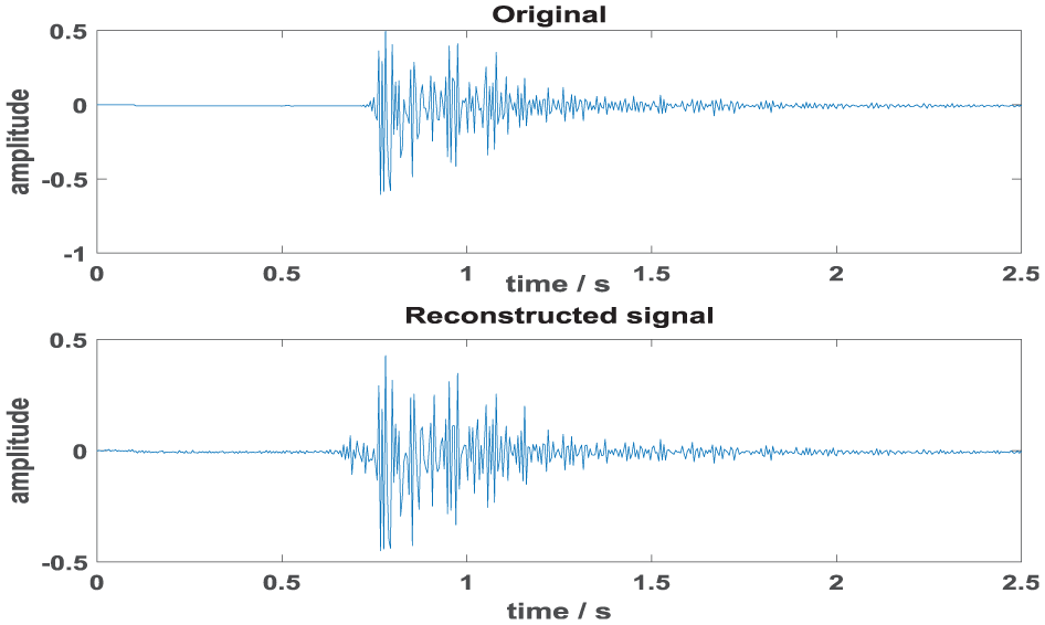
The sound signal after denoising using IVMD-wavelet algorithm with a noise level of 20 dB.

From Figures 9 to 12, it can be seen that the IVMD-wavelet threshold reconstruction after denoising results in a smoother waveform of the sound signal, retaining the main features of the sound signal while removing most of the noise. Applying this method to denoise multiple sets of collected acoustic signals can achieve good results.

Experiment 2

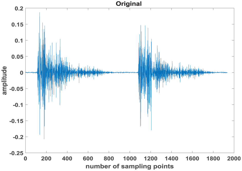
To verify the universality of the IVMD-wavelet algorithm, this experiment uses the acoustic signal of a three-phase induction motor during normal operation as the original acoustic signal. Then, Add 20 dB noise to the original signal, with a ratio of 7:3 between random Gaussian white noise and mechanical noise (i.e. pink noise). The IVMD algorithm is applied to decompose the noisy signal into five layers, and the correlation coefficient method is used to filter the IMF. The processed components are subjected to wavelet threshold filtering before reconstruction, and then the IVMD-wavelet algorithm is used to reconstruct the two processed components to form a denoised acoustic signal. The detailed diagram of the target signal and noise is shown in Figure 13.

Figure 13.

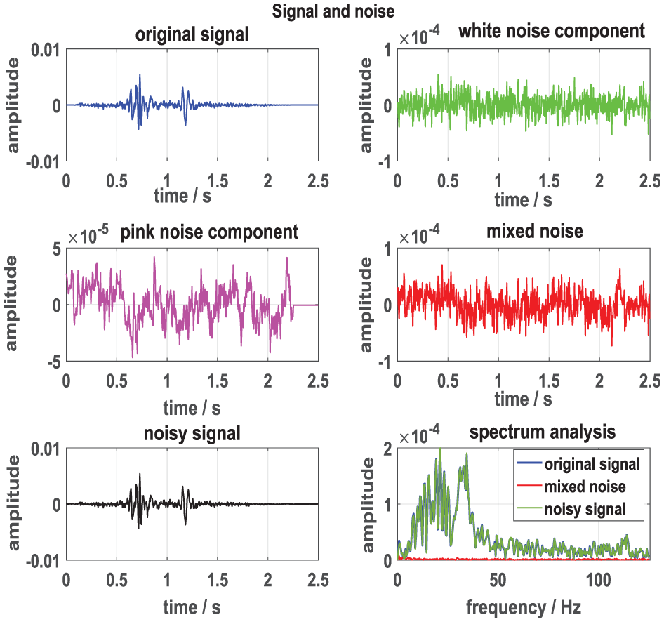
Original signal, mixed noise, and noisy signal.

Calculate the best effective rank order k of the singular value, and calculate it to be k = 5, which is the five-layer modal decomposition of IVMD, as shown in Figure 14.

Figure 14.

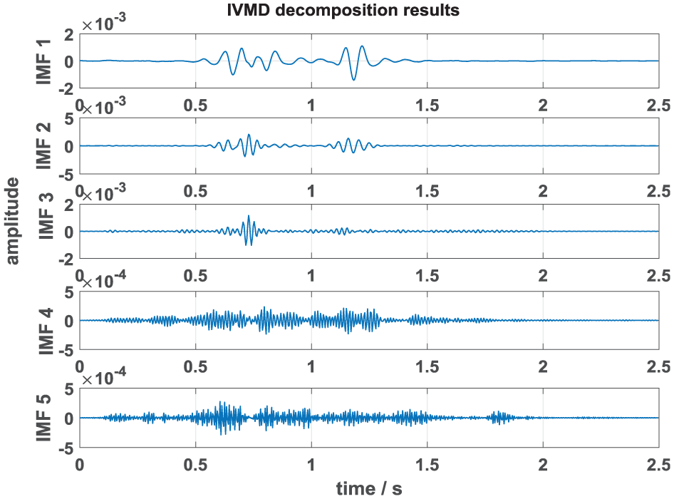
IVMD decomposition results.

Use the IVMD algorithm to decompose the noise-decomposed signal. The correlation coefficient between the IMF component and the signal is calculated, and after filtering, the effective IMF component and the to-process IMF component are extracted, and the to-processed IMF component is applied to the db5 wavelet threshold denoising. The obtained effective IMF component and wavelet threshold denoising component are reconstructed to obtain the denoised reconstruction signal, as shown in Figure 15.

Figure 15.

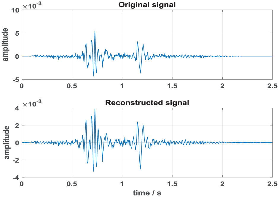
Comparison diagram of the original signal and the reconstructed signal.

From the experimental results, the SNR after denoising is 38.97, MSE = 0.000000, and RMSE = 0.000201. The denoising effect on the signal of a three-phase asynchronous motor is very good, proving the feasibility and universality of the method. We changed the SNR of the added noise and observed the denoising effect of the algorithm. The summary is shown in Table 2.

Table 2.

The denoising effect of IVMD algorithm under different noises.

	Evaluation result (dB)
Evaluation index	Add mixed noise by 5 dB	Add mixed noise by 10 dB	Add mixed noise by 20 dB
SNR	19.02	27.41	38.97
RMSE	0.000320	0.000254	0.000201

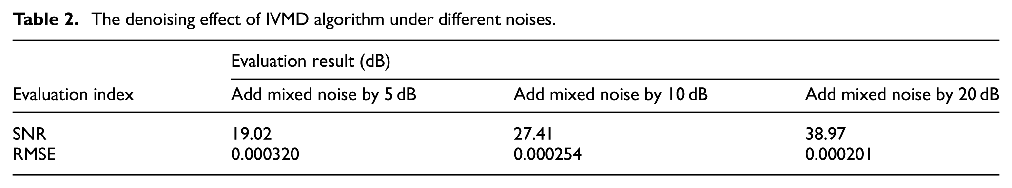
As can be seen from Table 2, the algorithm has a very good and stable denoising effect under different noise conditions. Our algorithm adaptively determines the parameters of VMD, such as α and the decomposition level K. To verify the feasibility of our selected parameters, we changed the parameter α and the number of layers K and continued to conduct experimental verification. The experimental results showed that the larger the parameter α, the better the denoising effect. However, if α is too large, signal distortion may occur, and the noise signal disappears but some useful signals are eliminated, resulting in a large root mean square error. When α is too small, the SNR is low, the denoising effect is poor, and compared with the original signal, the root mean square error is also relatively large. We selected α = 2000–2500 through algorithms and experiments. Hundreds of experiments have also verified that the method of determining K by the IVMD-wavelet algorithm in this paper is correct, effective, and feasible. This algorithm takes 0.02 s and can process signals quickly.

Experiment 3

Collect the sound signal of the firecracker as the original signal, add Gaussian white noise with a variance of 0.03 to form the noisy audio signal, as shown in Figure 16. Filter the noisy sound signal by using methods such as EEMD, VMD, db5 wavelet threshold denoising, and IVMD-db5 wavelet reconstruction denoising.

Figure 16.

The original sound signal in a noisy environment.

As shown in Figure 17, db5 wavelet fixed threshold denoising has the advantage of a “signal microscope,” which can effectively distinguish between effective signals and noise. The denoising effect is obvious, but the signal loss is severe. The denoising effect of EEMD is average and cannot suppress most of the noise. The VMD method has advantages in narrowband signal extraction, with smooth and distortion free signals after noise removal, but the noise recognition ability of VMD is weak. Compared with VMD algorithm, IVMD-wavelet reconstruction denoising algorithm fully utilizes the advantages of wavelet and VMD, and compensates for their shortcomings. The processing results show that the useful signal and noise are completely separated, the noise is basically removed, and the extracted signal is smooth and distortion free. Moreover, the adaptive selection of modal decomposition number and IMF component in this algorithm can more effectively express the original signal, which is closest to the noise free reference signal.

Figure 17.

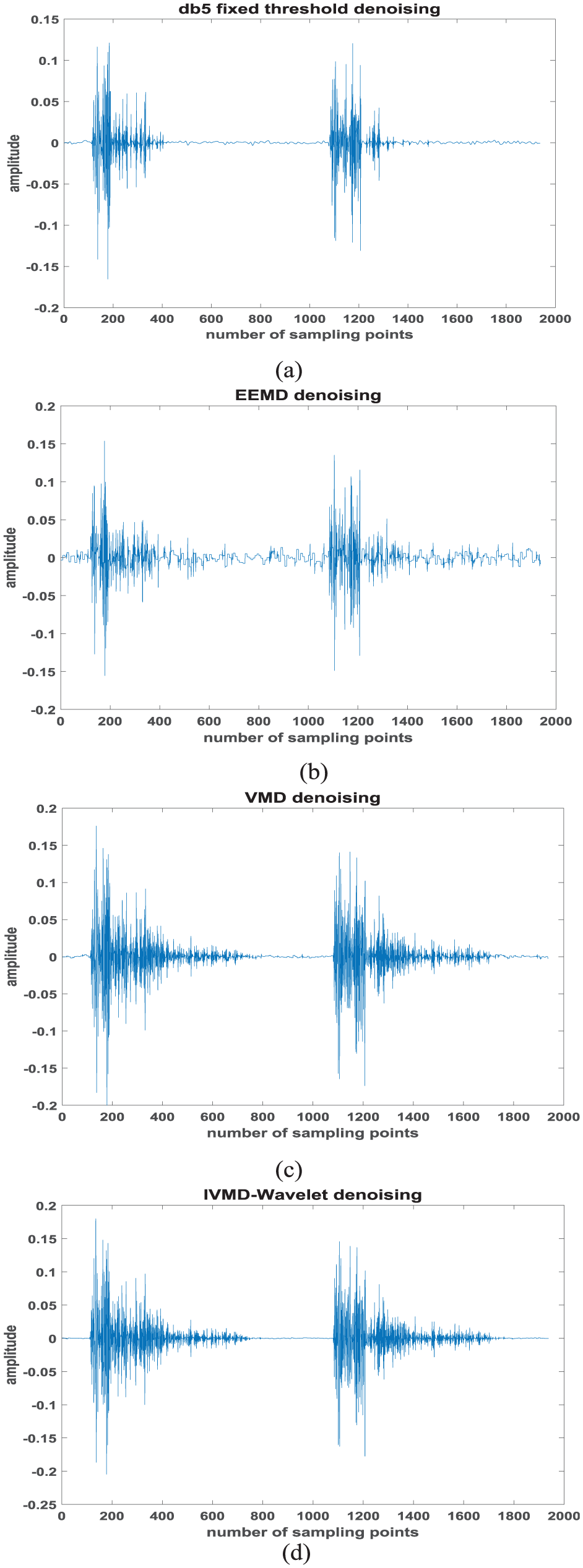
Comparison results of using different denoising algorithms on the same signal: (a) db5 algorithm; (b) EEMD algorithm; (c)VMD algorithm; (d) IVMD-db5 algorithm.

The SNR and RMSE of the signal are important indicators to measure the denoising degree of the algorithm. The calculation formula is as follows:

SNR = 10 \lg \frac{\sum_{i = 1}^{N} y_{i}^{2}}{\sum_{i = 1}^{N} {(y_{i} - {\hat{y}}_{i})}^{2}}

(21)

RMSE = \sqrt{\frac{1}{N} \sum_{i = 1}^{N} {(y_{i} - {\hat{y}}_{i})}^{2}}

(22)

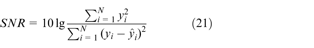
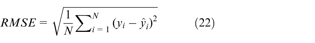
Where, y_i is the collected noisy signal; ${\hat{y}}_{i}$ is the sampled average filtered signal; N is the signal length.

To rigorously benchmark the performance of the proposed IVMD-wavelet algorithm, we compared it against three established methods: db5 wavelet hard thresholding, EEMD denoising, and standard VMD denoising. The original firecracker sound signal was used, and Gaussian white noise with a variance of 0.03 was added to create a noisy signal with an initial SNR of 15.72 dB, shown as Figure 16. For a statistically sound comparison, each denoising algorithm was applied to 100 independently generated noisy realizations of the original signal. The average SNR and RMSE results, along with their standard deviations, are reported in Table 3.

Table 3.

Comparative analysis of denoising performance across different algorithms (mean ± standard deviation over 100 trials).

Denoising method	SNR (dB)	RMSE
Original signal	15.72 ± 0.51	0.3564 ± 0.0211
Wavelet (db5)	29.35 ± 0.89	0.0972 ± 0.0085
EEMD	26.56 ± 1.24	0.1211 ± 0.0123
VMD	27.42 ± 1.05	0.0732 ± 0.0091
Proposed IVMD-wavelet	34.57 ± 0.61	0.0302 ± 0.0032

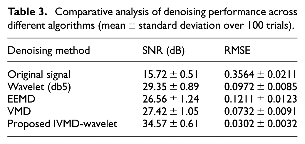
The results unequivocally demonstrate the superiority of the proposed method. Our IVMD-wavelet algorithm achieves the highest SNR and the lowest RMSE, with the smallest standard deviations, indicating superior and more consistent performance. The visual results in Figure 17 further corroborate this: while wavelet denoising causes some signal loss, and EEMD/VMD leave residual noise, the IVMD-wavelet output is smooth and retains the essential signal features.

To further investigate robustness against varying noise levels, we conducted a comprehensive test. According to equations (21) and (22), the SNR and RMSE of the signal processed by the four denoising methods are calculated, and the effects of different denoising methods are analyzed. The denoising indicators of different denoising methods are shown in Table 4.

Table 4.

Denoising performance under different input noise levels (mean ± standard deviation).

		Evaluation result (dB)
Denoising method	Evaluation index	Add noise by 5 dB	Add noise by 10 dB	Add noise by 20 dB
Wavelet	SNR	6.42 ± 0.71	13.03 ± 0.65	23.14 ± 0.58
Wavelet	RMSE	0.1227 ± 0.0102	0.0962 ± 0.0078	0.0728 ± 0.0061
EEMD	SNR	7.16 ± 0.95	15.90 ± 0.88	26.98 ± 0.79
EEMD	RMSE	0.1131 ± 0.0115	0.0849 ± 0.0091	0.0635 ± 0.0072
VMD	SNR	8.42 ± 0.82	16.64 ± 0.75	28.98 ± 0.69
VMD	RMSE	0.1032 ± 0.0098	0.0743 ± 0.0082	0.0525 ± 0.0065
IVMD- wavelet	SNR	10.30 ± 0.55	19.58 ± 0.50	37.72 ± 0.45
IVMD- wavelet	RMSE	0.0885 ± 0.0063	0.0564 ± 0.0051	0.0304 ± 0.0028

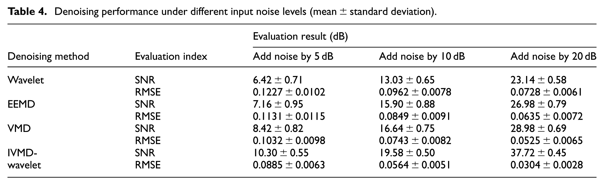
The data in Table 4 confirms that the proposed algorithm consistently outperforms the benchmark methods across all tested noise levels. Quantitatively, compared to EEMD denoising, our method improves the SNR by an average of 28% and reduces the RMSE by an average of 52%. This significant enhancement stems from the synergistic effect of the adaptive VMD decomposition, which cleanly separates signal and noise modes, and the targeted wavelet denoising, which efficiently suppresses noise in the residual components without distorting the signal.

Conclusions

Aiming at the acoustic localization of target objects in complex environments, a denoising method based on IVMD-wavelet reconstruction is proposed to address the instability of acoustic signals and their susceptibility to background noises, such as environmental noise and vehicle noise. We conducted three experiments using different types of signals. For different types of noise, the algorithm proposed in this paper can quickly denoise them. Experiments demonstrate that the proposed algorithm achieves a small RMSE. Our algorithm adaptively determines the parameters of IVMD, such as α and the decomposition level K. To verify the feasibility of our selected parameters, we changed the parameter α and the number of layers K and continued to conduct experimental verification. The experimental results showed that the larger the parameter α, the better the denoising effect. However, if α is too large, signal distortion may occur, and the noise signal disappears but some useful signals are eliminated, resulting in a large root mean square error. When α is too small, the SNR is low, the denoising effect is poor, and compared with the original signal, the root mean square error is also relatively large. When K is large, excessive decomposition occurs. When K is small, insufficient decomposition happens. Therefore, this algorithm can solve this problem. The algorithm in this paper adaptively determines the number of decomposition layers K through the SVD method. Hundreds of experiments have also verified that the method of determining K by the IVMD-wavelet algorithm in this paper is correct, effective and feasible. Compared with EEMD threshold denoising, the signal SNR processed by the proposed algorithm is increased by 28%, and the RMSE is reduced by 52%. The fully adaptive nature of the algorithm, coupled with its robust performance across different noise types and levels, makes it a highly suitable and effective tool for practical acoustic signal processing applications.

Footnotes

ORCID iD

Xuewei Zhang

Ethical considerations

This article does not contain any studies with human or animal participants. There are no conflicts of interest, and it is original and it has not been submitted elsewhere in any form or language.

Consent to participate

All authors have read and approved to submit it to your journal.

Consent for publication

Not applicable.

Author contributions

Conceptualization, X.Z.; methodology, X.Z.; software, C.Z.; validation, X.Z., C.Z and X.S.; formal analysis, C.Z.; investigation, X.S.; resources, X.Z.; data curation X.S.; writing—original draft preparation, X.Z.; writing—review and editing, X.Z.; visualization, X.S.; supervision, C.Z.; project administration, X.Z.; funding acquisition, X.Z. All authors have read and agreed to the published version of the manuscript.

Funding

The authors disclosed receipt of the following financial support for the research, authorship, and/or publication of this article: This work has been supported by the Natural Science Foundation of Shaanxi Provincial Department of Science and Technology (2025JC-YBMS-483).

Declaration of conflicting interests

The authors declared no potential conflicts of interest with respect to the research, authorship, and/or publication of this article.

Data availability statement

The datasets generated during and/or analyzed during the current study are available from the corresponding author on reasonable request.

References

Liu

Duan

Seismic signal denoising using f-x variational mode decomposition. IEEE Geosci Remote Sens Lett 2020; 17(8): 1313–1317.

Jin

Wang

Non-local means image denoising with a soft threshold. IEEE Signal Process Lett 2015; 22(7): 833–837.

Lin

, et al. EMG signal filtering based on variational mode decomposition and sub-band thresholding. IEEE J Biomed Health Inform 2021; 25(1): 47–58.

Zhang

Zhong

, et al. Detection for incipient damages of wind turbine rolling bearing based on VMD-AMCKD method. IEEE Access 2019; 7: 67944–67959.

Aneesh

Kumar

Hisham

, et al. Performance comparison of variational mode decomposition over empirical wavelet transform for the classification of power quality disturbances using support vector machine. Procedia Comput Sci 2015; 46: 372–380.

Sun

Huang

A hybrid air pollutant concentration prediction model combining secondary decomposition and sequence reconstruction. Environ Pollut 2020; 266(3): 115216.

Zhang

Liu

, et al. An adaptive CEEMDAN thresholding denoising method optimized by nonlocal means algorithm. IEEE Trans Instrum Meas 2020; 69(9): 6891–6903.

Ting-ting

Yan

Zong

, et al. A fault diagnosis method of rolling bearing based on VMD Tsallis entropy and FCM clustering. Multimed Tools Appl 2020; 79(39–40): 30069–30085.

Wang

Zhang

Cao

, et al. A rolling bearing fault diagnosis method based on the WOA-VMD and the GAT. Entropy 2023; 25(6): 889.

10.

Krishnamani

P.a K Swaminathan

Variational mode decomposition based differentiation of fatigue conditions in muscles using surface electromyography signals. IET Signal Process 2020; 14(10): 745–753.

11.

Yue

Zhu

, et al. An improved variational mode decomposition method based on the optimization of salp swarm algorithm used for denoising of natural gas pipeline leakage signal. Measurement 2021; 185: 110107.

12.

Cui

Guan

Chen

Rolling element fault diagnosis based on VMD and sensitivity MCKD. IEEE Access 2021; 9: 120297–120308.

13.

Yue

Zhu

, et al. Variational mode decomposition denoising combined with improved Bhattacharyya distance. Measurement 2020; 151: 107283.

14.

Gao

Zhu

Cai

, et al. Pattern recognition of partial discharge based on VMD-CWD spectrum and optimized CNN with cross-layer feature fusion. IEEE Access 2020; 8: 151296–151306.

15.

ur Rehman

Safdar

ur Rehman

, et al. Dynamically sampled bivariate empirical mode decomposition. IEEE Signal Process Lett 2014; 21(7): 857–861.

16.

Huang

Shen

Long

, et al. The empirical mode decomposition and the Hilbert spectrum for nonlinear and non-stationary time series analysis. Proc R Soc Lond Sér Math Phys Eng Sci 1998; 454(1971): 903–995.

17.

Chien

Wang

Shi

, et al. Noise suppression: empirical modal decomposition in non-dispersive infrared gas detection systems. Infrared Phys Technol 2020; 108: 103335.

18.

Oberlin

Meignen

Perrier

An alternative formulation for the empirical mode decomposition. IEEE Trans Signal Process 2012; 60(5): 2236–2246.

19.

Wang

Zhao

Filter bank properties of envelope modified EMD methods. IET Signal Process 2018; 12(7): 844–851.

20.

Huang

NE.

Ensemble empirical mode decomposition: a noise-assisted data analysis method. Adv Adapt Data Anal 2009; 1(01): 1–41.

21.

Sezen

Pan evaporation forecasting using empirical and ensemble empirical mode decomposition (EEMD) based data-driven models in the Euphrates sub-basin, Turkey. Earth Sci Inform 2023; 16(4): 3077–3095.

22.

Jalal

Yang

Liu

, et al. Fast and robust variable-step-size LMS algorithm for adaptive beamforming. IEEE Antennas Wirel Propag Lett 2020; 19(7): 1206–1210.

23.

Fang

Zhang

, et al. Comparison of EMD and EEMD in rolling bearing fault signal analysis. In: 2018 IEEE international instrumentation and measurement technology conference (I2MTC): discovering new horizons in instrumentation and measurement, 2018, pp. 737–741.

24.

Yeh

Shieh

Huang

NE.

A complete ensemble empirical mode decomposition with adaptive noise and its application to rolling element bearing fault diagnosis. Adv Adapt Data Anal 2010; 2(02): 135–156.

25.

Torres

Colominas

Schlotthauer

, et al. A complete ensemble empirical mode decomposition with adaptive noise. In: 2011 IEEE international conference on acoustics, speech and signal processing (ICASSP), Prague, Czech Republic, 2011, pp. 4144–4147.

26.

Dragomiretskiy

Zosso

. Variational mode decomposition. IEEE Trans Signal Process 2014; 62(3): 531–544.

Research on reconstruction and processing methods for complex acoustic signals

Abstract

Keywords

Introduction

Signal denoising method based onIVMD-wavelet transform algorithm

The IVMD model of complex environmental acoustic signals

Calculation method of modal number based on SVD

Modal component selection based on cross-correlation coefficient

Filtering and processing method of complex acoustic signal based on wavelet transform

A denoising method for complex acoustic signals based on IVMD-wavelet

Calculation and experimental analysis

Calculation of the optimal mode number K

Screening of IMF components in IVMD

Screening of IMF components in IVMD

Evaluation of denoising performance of IVMD-wavelet reconstruction algorithm

Experiment 1

Experiment 2

Experiment 3

Conclusions

Footnotes

ORCID iD

Ethical considerations

Consent to participate

Consent for publication

Author contributions

Funding

Declaration of conflicting interests

Data availability statement

References