Sage Journals: Discover world-class research

Abstract

Training performance of athletes relies on the training initiative, which in turn is related to the construction of training plans. To forecast training performance of athletes, based on the Event-group training theory, this paper proposed a novel forecast method through combining with the discrete Hopfield neural network and wavelet function. The critical principle is that using Event-group training theory to construct 13 training indicators for athletes. The training scores of athletes is calculated by the constructed 13 training indicators. According to the designed training indicators, the discrete Hopfield neural network with wavelet function is implemented. In process of model training, to complete quick convergence and to guarantee the stability of state update to our discrete Hopfield neural network, the designed wavelet function is taken. Following that, the proposed model is trained by using the experimental dataset, and using the trained model to forecast the training performance of athletes. Experimental results show that the proposed model not only accurately forecasts the training performance of athletes, but also outperformed the comparative models in forecast accuracy. Results also show that the running efficiency of the proposed model won major competitors. The value of the designed training indicators not only finds these major factors affecting training performance of athletes, but also assists coaches in scientifically specifying training plans and observing athletes’ training performance.

Keywords

performance forecast neural networks athletic training

Introduction

Training performance of athletes is a key indicator to measure the training effectiveness and competitive ability. The quality of training results directly affects whether athletes can achieve excellent results in competitions. Therefore, analyzing and improving training performance of athletes is an important means to improve their overall strength and strive for good results.

There are many factors affecting athletes’ training results,¹ including (i) physical fitness, which is the foundation of athletes’ training results, such as strength, speed, endurance, and so on. Among them, the speed and strength factors have the greatest contribution to the 100-m performance. Therefore, for 100-m athletes to achieve excellent results, they not only need to undergo training in index factors, absolute speed factors, and speed endurance factors, but more importantly, they need to strengthen the training of speed and strength factors, which is the key to improving performance. (ii) Training process, which has a significant impact on the performance of athletes. For example, female endurance athletes use a training format being like male athletes, but often the absolute amount of their exercise is lower than that of male athletes. If the training load is exceeded, it has almost no effect on improving grades. (iii) Psychological quality, which is regarded as another important factor affecting the training performance of athletes. Modern competitive sports are becoming more and more intense. The positive or negative emotions of athletes can both affect their technical level and the results of the competition.

The Event-group training theory^2,3 is highly favored in training athletes. The Event-group training theory (also namely, Xiang-qun training theory), which was proposed based on the general training theory and specialized training theory of competitive sports, takes the similarities and differences between projects caused by the essential attributes of different projects as a basis, and compares and studies a group of sports projects with similar competitive characteristics and training requirements together. The Event-group training theory indicates that basic tasks of training activities are to improve and develop the competitive abilities of athletes. For instance, Ref.⁴ proposed an optimization algorithm to analysis of sport performance according to the Event-group training theory. And the method proposed by Ref.⁵.

Motivation

The goals in this paper are to forecast training performance of athletes, and to find the critical factors affecting the training performance. To complete the study goals, according to the Event-group training theory, this paper firstly constructed 13 training indicators, then, the discrete Hopfield neural network with wavelet function (i.e., namely DHNN-WF) is proposed based on the constructed 13 training indicators. On the one hand, from the model level, discrete Hopfield neural networks have natural ascendency in terms of the forecast, while they have a risk of weak convergence. In process of the training, to achieve quick convergence and to guarantee the stability of state update to of our discrete Hopfield neural network, the designed wavelet function is used for it. On the other hand, using the constructed 13 training indicators to calculate the training scores of athletes, together, the constructed 13 training indicators and the calculated training scores are used to train the proposed model. By doing so, the proposed model can accurately predict training performance of athletes.

Contributions

We summarized the main contributions in this work. As follows

(1) The training indicators were designed based on the Event-group training theory. through calculating the correlation between the training indicators and the training performance predicted by the proposed model, we obtained the major training indicators affecting training performance of athletes.

(2) According to the designed training indicators, this work proposed the discrete Hopfield neural network with wavelet function. Through utilizing the constructed wavelet function, the convergence of the discrete Hopfield neural network is improved. This effectively guarantees the forecast ability of the proposed model.

(3) Using the major training indicators affecting training performance of athletes can efficiently specify training plans. The value of the designed training indicators lies in their ability to assist coaches in scientifically observing athletes’ training performance and adjusting training plans in real-time.

Related works

Recently, these studied findings about training performance of athletes have been proposed. For example, Sonu et al.⁶ utilized machine Learning technique to analyze the health condition of athletes and to forecast their performance. Sonu et al. applied various machine learning algorithms random forest, logistic regression, gradient boosting, decision tree classifier and K-neighbors classifier to forecast athlete’ performance, however, results show that random forest classifier is more suitable for the analytic of athlete’ health and performance. For the characteristics of modern sports, Nan⁷ took the principle of artificial intelligence sensor as the basic basis to accurately analyze the physical state of athlete’ training, then using the analyzed results to promote the improvement of athletic performance. The proposed method is proved to be success in the forecast for athletic performance, however, the method must rely on a sensor instrument to collect the athletic data. Additionally, the supervised machine learning method proposed by Ref.⁸ is used for athlete-monitoring, which accurately obtains the athletic data during the training. Zhu et al.⁹ apply the Bayesian Method (BM) to recognize incorrect movements of athletes, and the recognized results provide assistances for coaches to specify training plans. Similarly, using machine learning methods and artificial intelligent methods to analyze the performance of athletes, including the 3D visualization technology proposed by Ref.¹⁰ for athletes training. Ping et al.¹¹ designed the Hidden Markov Model (HMM) based on blockchain mechanism to complete sport performance prediction for athletes. The HMM model can cope with the data sparsity and dynamics, but the training of the HMM model needs to a large amount of past exercise data to obtain superior forecast performance. To objectively evaluate the performance of diving sport actions in a continuous video stream, Pramod et al.¹² utilized a hybrid mechanism consisting of multiple models, So, the hybrid mechanism consumes much training time. Erica et al.¹³ developed a dynamic online dashboard for tracking the performance of athletic performance. Using a simple color-coded designed scheme to convey the details to the coaches. Christine et al.¹⁴ implemented a web framework for athlete profiling and training load monitoring. With the assistance of the web framework, coaches can examine and evaluate their athletes’ condition, so as to maximize the development of the athlete training load. The machine learning algorithms in Refs^15–22 successfully forecast athlete training performance. Whether machine learning or artificial intelligence methods yield satisfactory results in forecasting or analyzing athletic performance.

Raj et al.²³ employed Hopfield neural networks for prediction tasks, achieving an accuracy of 92.41%. To address training requirements, Simone et al.²⁴ utilized a continuous-time Hopfield model and generalized the sign activation function to incorporate saturation at arbitrary points, significantly enhancing the model’s predictive capability. For continuous self-learning control systems, Tan et al.²⁵ adapted the Hopfield neural network framework for achievement prediction. Na et al.²⁶ further improved the forecasting and analytical capacities of Hopfield networks by introducing hyperbolic tangent memristors and quadratic nonlinear memristors, demonstrating their potential in data processing, image encryption, and biomedical applications. Additional studies in Refs.^27–29 effectively leveraged the robust prediction and analytical strengths of Hopfield neural networks.

Beyond Hopfield networks, Zhu et al.³⁰ designed a Wavelet Neural Network-based prediction method, combining wavelet transform advantages with neural networks’ learning ability to address low accuracy and efficiency. In contrast, Gao et al.³¹ proposed a roughness prediction method using Wavelet Transform and Convolutional Neural Networks for offline applications. Similarly, Quan et al.³² integrated Long Short-Term Memory neural networks with wavelet analytics for prediction problems. Other studies (Refs.^33–35) adopted comparable hybrid approaches combining wavelet techniques with neural networks.

Methods

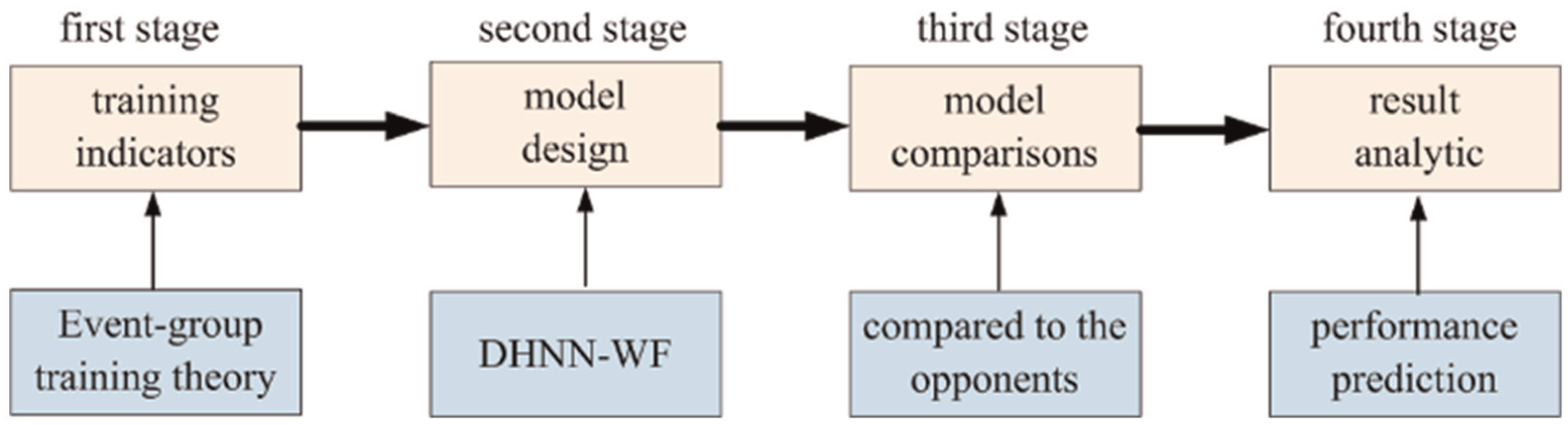
This section illustrates the design of the 13 training indicators. Then, the discrete Hopfield neural network with wavelet function (i.e., namely DHNN-WF) is implemented. To the method in detail, the overall scheme is firstly given in Figure 1.

Figure 1.

The proposed scheme.

Overall scheme

Figure 1 displays the overall scheme of the method, including the design of training indicators, model implementation, model comparison, and result analytic. In the first stage, using the Event-group training theory to design 13 training indicators. Then, the dataset based on the 13 training indicators was into a training set, a testing set and a validation set. The testing set is used for parameter verification of the model, and the validation set is the validation of forecast ability to the model. The task in second stage is the design of the model. We took account into the discrete Hopfield neural network, and designed a wavelet function. In third stage, the proposed model is compared to the opponents to evaluate our forecast ability. Finally, the forecast results were discussed in the fourth stage.

Training indicators based on event-group training theory

The Event-group training theory indicates that physical fitness competitions should possess fast strength, speed, and endurance, and the skill competitions should have performance perfection, performance accuracy, confrontation in the same field. According to the Event-group training theory and taking the suggestions of Ref.² and Ref.³ as a reference, this work considered five training groups, including load structure training group, metabolic ability training group, skeletal muscle strength training group, regional effect training group, and recovery training group. Then, corresponding training indicators were designed for each training group, specifically, including 13 training indicators, as shown in Table 1.

Table 1.

Deals of 13 training indicators.

Group 1	Group 2	Group 3	Group 4	Group 5
Load structure training group	Metabolic ability training group	Skeletal muscle strength training group	Regional effect training group	Recovery training group
S-TC (short-term continuous training) (10 min)	AET (aerobic training) (30 min)	MSE (moderate strength endurance) (5 min)	BFT (barrier free training) (30 min)	S-TPR (short-term physical recovery) (10 min)
M-TC (medium-term continuous training) (30 min)	ANT (anaerobic training) (30 min)	LSE (long-term strength endurance) (10 min)	OBT (obstacle training) (30 min)	L-TPR (long-term physical recovery) (30 min)
L-TC (long-term continuous training) (60 min)	HYT (hybrid training) (30 min)		BET (beach training) (30 min)

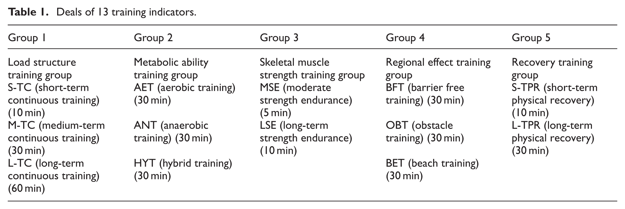
Group 1, load structure training group. In this group, three indicators were considered, including short-term continuous (S-TC) training, medium-term continuous (M-TC) training, and long-term continuous (L-TC) training. S-TC training requires a load time of 10 min for each continuous training session. M-TC training keeps a load time of 30 min for each continuous training session. However, L-TC training must keep a load time of 60 min for each continuous training session.

Group 2, metabolic ability training group, which includes aerobic training (AET), anaerobic training (ANT), and hybrid training (HYT) of aerobic and anaerobic training. The training time of the three training manners is 30 min.

Group 3, skeletal muscle strength training group. According to the duration of the competition, it can be divided into moderate strength endurance (MSE) training and long-term strength endurance (LSE) training. MSE training and LSE training require 4 and 8 min.

Group 4, regional effect training group. In the group, utilizing different training conditions, barrier free training (BFT), obstacle training (OBT), and beach training (BET) were set up. Their training time is set up 30 min.

Group 5, recovery training group, which mainly promotes the recovery of athletes after the training, including short-term physical recovery (S-TPR) and long-term physical recovery (L-TPR). S-TPR and L-TPR spend 10 min, 30 min, respectively.

Model design

Model structure

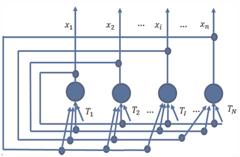
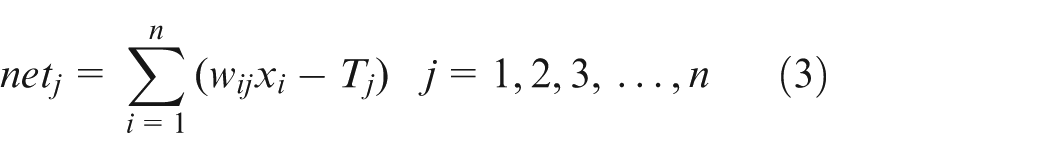
The discrete Hopfield neural network is used as the model. Figure 2 displays the structure, showing that it is a single-layer full feedback network with n neurons. The output x_i of any neuron receives feedback from all neurons through connection weights, and this is to ensure that each neuron is controlled by the outputs of all neurons, thereby constraining the outputs of each other. Each neuron has a threshold T_j to reflect the control of input noise.

Figure 2.

The structure of the discrete Hopfield neural network.

Each neuron in the network has the same function, and its output is called a state, denoted as x_j. The state of the feedback network composed of all neuron states is $X = [x_{1}, x_{2}, . . . . . ., x_{n}]^{T}$ . The initial state of the feedback network is represented as $X (0) = [x_{1} (0), x_{2} (0), . . . . . ., x_{n} (0)]^{T}$ . Once the initial value is given, the network begins to dynamically evolve. The state of each neuron in the network is changed, as follows,

x_{j} = f (ne t_{j}) j = 1, 2, 3, \dots, n

(1)

Where $f (ne t_{j})$ is the activation function (transfer function), having that

f (ne t_{j}) = {\begin{matrix} 1, ne t_{j} \geq 0 \\ - 1, ne t_{j} < 0 \end{matrix} j = 1, 2, 3, \dots, n

(2)

The $ne t_{j}$ is calculated by equation (3).

ne t_{j} = \sum_{i = 1}^{n} (w_{ij} x_{i} - T_{j}) j = 1, 2, 3, \dots, n

(3)

Where $w_{ii} = 0$ and $w_{ij} = w_{ji}$ . When the state of each neuron in the network is not changing, the transition state is the output state of the network, as follows,

\lim_{t \to \infty} x (t)

(4)

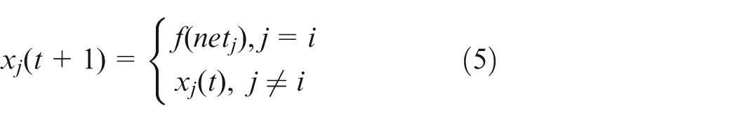
During the running of network, one neuron updates the state, while the state weights of other neurons remain unchanged. As follows,

x_{j} (t + 1) = {\begin{matrix} f (ne t_{j}), j = i \\ x_{j} (t), j \neq i \end{matrix}

(5)

The network starts from the initial state $x (0)$ , after it undergoes finite recursion, the state does not change anymore, that is, $x (t + 1) = x (t)$ , thereby reaching a stable state.

Wavelet function

The selection of a wavelet function is related to the nature of the data and analysis goals. Some wavelets are more regular (smooth) while others are less so. Regular wavelets are better for analyzing smooth data, while less regular wavelets can capture discontinuities. Orthogonal wavelets maintain energy conservation and are often used in data compression and denoising. Biorthogonal wavelets offer more flexibility in handling non-stationary signals but do not conserve energy perfectly. For example,

Haar wavelet, which has simplest wavelet with a compact support, and good for detecting abrupt changes.

Daubechies (db) wavelet, which offers different orders (db1, db2, etc.) with varying degrees of smoothness and compact support, and suitable for general-purpose signal analysis.

Symlet wavelet, which is similar to Daubechies but more symmetric, useful for analyzing signals with asymmetric features.

Coiflet wavelet, which provides better time localization and are suitable for analyzing signals with fast transients.

Morlet wavelet, which is often used in continuous wavelet transforms for time-frequency analysis, particularly in applications like EEG signals.

Meyer wavelet. Although it is not tight support, the convergence speed is fast, moreover, it is infinitely differentiable.

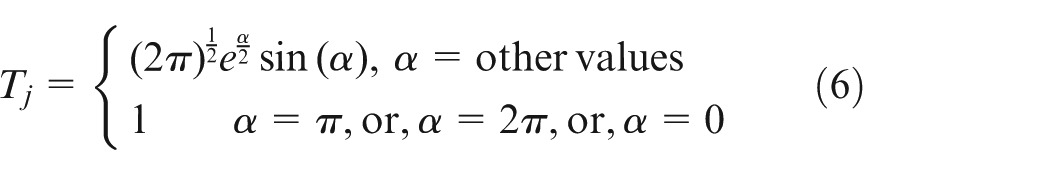
To achieve quick convergence of our model and quickly enter a stable state, according to quick convergence ascendency of Meyer wavelet function, we used the Meyer wavelet function to calculate the threshold T_j in equation (3), and $α \in [0, 2 π]$ . As follows,

T_{j} = {\begin{matrix} {(2 π)}^{\frac{1}{2}} e^{\frac{α}{2}} \sin (α), α = other values \\ 1 α = π, or, α = 2 π, or, α = 0 \end{matrix}

(6)

Consequently, the proposed DHNN-WF is given in equation (7)

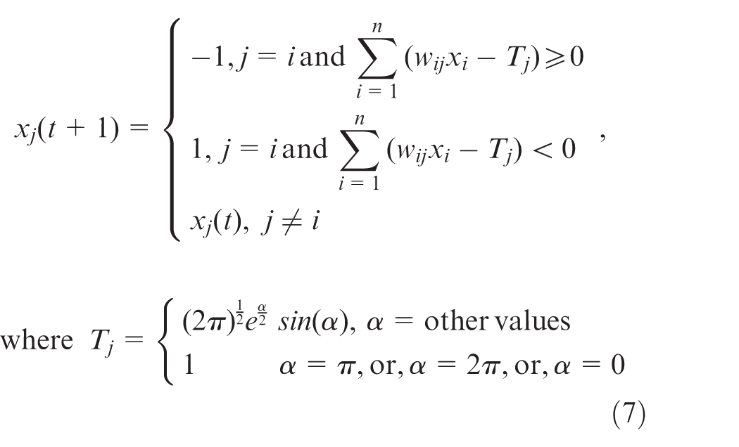
\begin{matrix} x_{j} (t + 1) = {\begin{matrix} - 1, j = i and \sum_{i = 1}^{n} (w_{ij} x_{i} - T_{j}) \geq 0 \\ 1, j = i and \sum_{i = 1}^{n} (w_{ij} x_{i} - T_{j}) < 0 \\ x_{j} (t), j \neq i \end{matrix}, \\ where T_{j} = {\begin{matrix} {(2 π)}^{\frac{1}{2}} e^{\frac{α}{2}} \sin (α), α = other values \\ 1 α = π, or, α = 2 π, or, α = 0 \end{matrix} \end{matrix}

(7)

Where $α \in [0, 2 π]$ , weight values $w_{ii} = 0$ and $w_{ij} = w_{ji}$ .

The Meyer wavelet provides an excellent balance between time and frequency localization due to its smoothness and orthogonality. The Meyer wavelet forms an orthonormal basis, ensuring that the wavelet coefficients are uncorrelated, improving feature discrimination. The Meyer wavelet’s smooth decay in frequency allows for stable gradient computations during backpropagation, increasing the adaptability to neural network training. Therefore, the Meyer wavelet is theoretically optimal for DHNN-WF due to its orthogonality, excellent frequency localization, and smoothness, all of which enhance feature extraction and network stability.

Parameter configuration

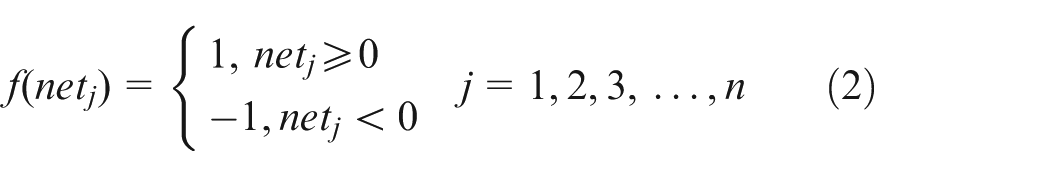
Configuration of neurons. Currently, it is difficult to find a general rule for configuring the number of neurons, and most existing methods utilize dynamic configuration of neuron numbers within a certain range. Hence, this paper adopts a dynamic adjustment of the number of neurons within a certain range. The initial configuration for the number of neurons is $\sqrt{| volume |}$ , where $| volume |$ is data volume of the input dataset. Through observing loss curve, we adjust the number of neurons within the range ${20, \dots, \sqrt{| volume |} - 50, \sqrt{| volume |} - 30, \sqrt{| volume |} - 10, \sqrt{| volume |} + 10, \sqrt{| volume |} + 30, \sqrt{| volume |} + 50}$ , then, we choose corresponding number of neurons when loss value is the lowest. This is to overcome overfitting or underfitting when there are too many or too few neurons.

Configuration of activate function. According to work principle of discrete Hopfield neural networks, $f (ne t_{j})$ in equation 2 is used as the activate function of our DHNN-WF.

Configuration of threshold T_j. The initial configuration for the threshold T_j is 1, and $[0, 2 π]$ is set as a time cycle. Threshold T_j is calculated by equation (6) within each time cycle.

Configuration of neuron weights. Combining equations (6) and (7), neuron weights are dynamically configured within each time cycle.

Model training

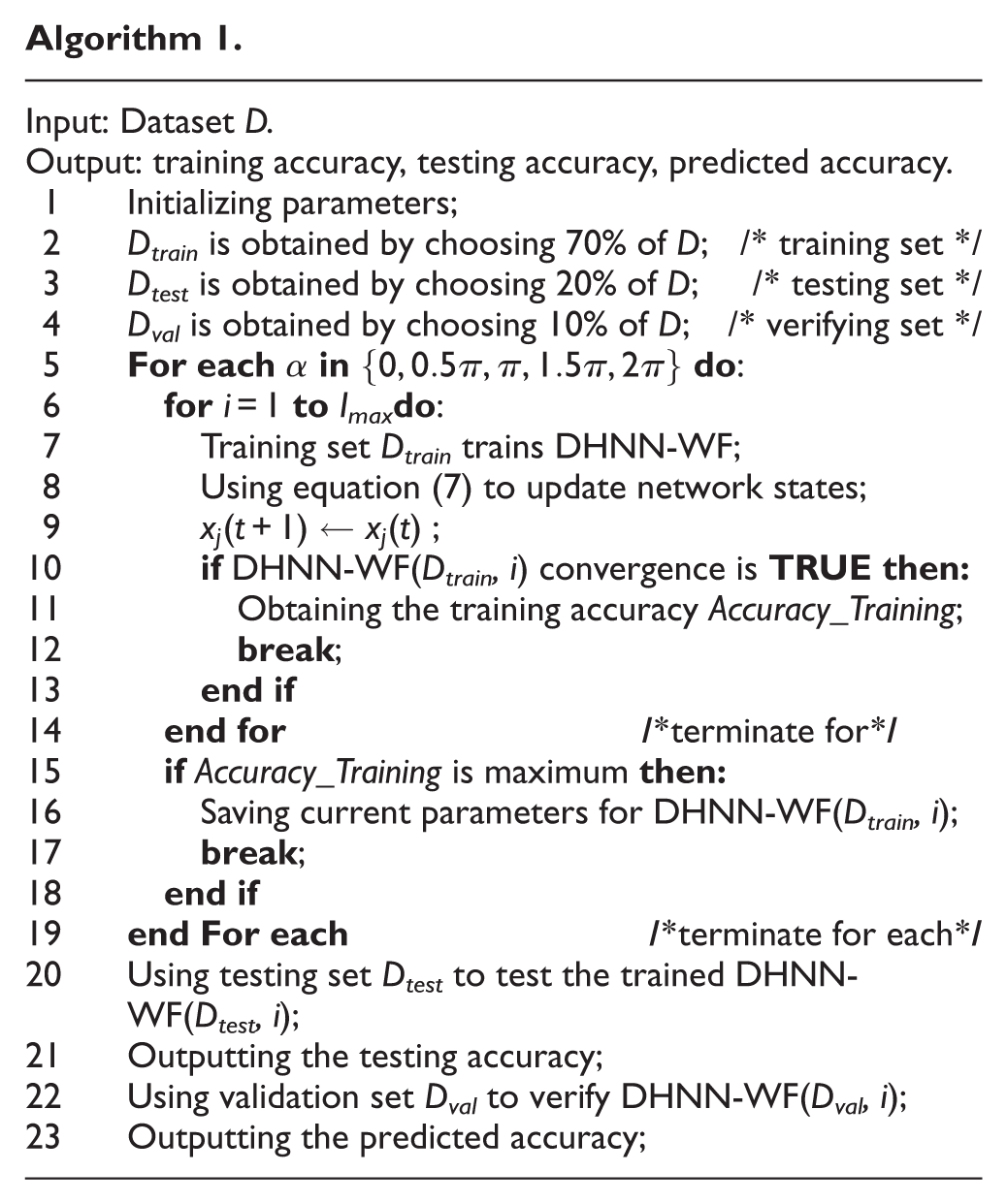
The training of the DHNN-WF is as shown in Algorithm 1. Dataset D is the input and the output is forecast accuracy. The parameters were initialized in Step 1. Then, Dataset D was divided into the training set D_train, the testing set D_test, and the validation set D_val, as shown in Step 2 to Step 4. The testing set D_test is used for network parameter verification of our DHNN-WF. The validation set D_val is used to verify the predicted ability of our DHNN-WF. After completing the division of the dataset D, the DHNN-WF is undergone iterative training in Step 5 to Step 18, where equation (7) is used for the network state update, illustrated in Step 8 and Step 9. Once our DHNN-WF reached a convergence state, the training is immediately terminated. Meanwhile, the current training parameters are saved, then the maximum training accuracy is outputted, illustrated in Step 10 to Step 18. Using testing set D_test to test the trained DHNN-WF, and the testing accuracy is outputted, as shown in Step 20 and Step 21. Finally, the forecast ability of the trained DHNN-WF is verify on the validation set D_val, illustrated in Step 22 and Step 23.

Algorithm 1.

Input: Dataset D.
Output: training accuracy, testing accuracy, predicted accuracy.
1	Initializing parameters;
2	D _train is obtained by choosing 70% of D; /* training set */
3	D _test is obtained by choosing 20% of D; /* testing set */
4	D _val is obtained by choosing 10% of D; /* verifying set */
5	For each $α$ in ${0, 0.5 π, π, 1.5 π, 2 π}$ do:
6	fori = 1 toI_maxdo:
7	Training set D_train trains DHNN-WF;
8	Using equation (7) to update network states;
9	$x_{j} (t + 1) \leftarrow x_{j} (t)$ ;
10	if DHNN-WF(D_train, i) convergence is TRUE then:
11	Obtaining the training accuracy Accuracy_Training;
12	break;
13	end if
14	end for /terminate for/
15	ifAccuracy_Training is maximum then:
16	Saving current parameters for DHNN-WF(D_train, i);
17	break;
18	end if
19	end For each /terminate for each/
20	Using testing set D_test to test the trained DHNN-WF(D_test, i);
21	Outputting the testing accuracy;
22	Using validation set D_val to verify DHNN-WF(D_val, i);
23	Outputting the predicted accuracy;

Experimental settings

Datasets

We collected the data from 1000 athletes within a training cycle according to Table 1, that is, a week represents a training cycle. The experimental dataset is as shown Table 2. Aiming for the eleven training indicators in the item groups 1–4, the results completed by the i-th athlete within a training cycle are marked with F( )_I and $1 \leq i \leq 1000$ . While for the two training indicators in the item group 5, after the athletes completed the recovery training, we monitor body indicators of the athletes by monitoring instruments. Then, we recorded the recovery time that body indicators, for example, heart rate, blood glucose concentration, and so on, can recover normal values. The average recovery time of the i-th athlete within a training cycle is denoted as T( )_i minutes.

Table 2.

Illustrations of experimental dataset.

		Athlete no.
Group		Athlete₁	…	Athlete_i	…	Athlete₁₀₀₀
1	S-TC	F(S)₁ = 6	…	F(S)_i	…	F(S)₁₀₀₀ = 10
	M-TC	F(M)₁ = 10	…	F(M)_i	…	F(M)₁₀₀₀ = 6
	L-TC	F(L)₁ = 10	…	F(L)_i	…	F(L)₁₀₀₀ = 10
2	AET	F(AE)₁ = 10	…	F(AE)_i	…	F(AE)₁₀₀₀ = 6
	ANT	F(AN)₁ = 6	…	F(AN)_i	…	F(AN)₁₀₀₀ = 6
	HYT	F(HY)₁ = 10	…	F(HY)_i	…	F(HY)₁₀₀₀ = 6
3	MSE	F(ME)₁ = 10	…	F(ME)_i	…	F(ME)₁₀₀₀ = 10
	LSE	F(LE)₁ = 6	…	F(LE)_i	…	F(LE)₁₀₀₀ = 10
4	BFT	F(FT)₁ = 10	…	F(FT)_i	…	F(FT)₁₀₀₀ = 10
	OBT	F(BT)₁ = 10	…	F(BT)_i	…	F(BT)₁₀₀₀ = 6
	BET	F(ET)₁ = 6	…	F(ET)_i	…	F(ET)₁₀₀₀ = 0
5	S-TPR	T(s-t)₁ = 10	…	T(s-t)_i	…	T(s-t)₁₀₀₀ = 10
	L-TPR	T(l-t)₁ = 10	…	T(l-t)_i	…	T(l-t)₁₀₀₀ = 6
Scores		S ₁ = 8.77	…	S _i	…	S ₁₀₀₀ = 7.38

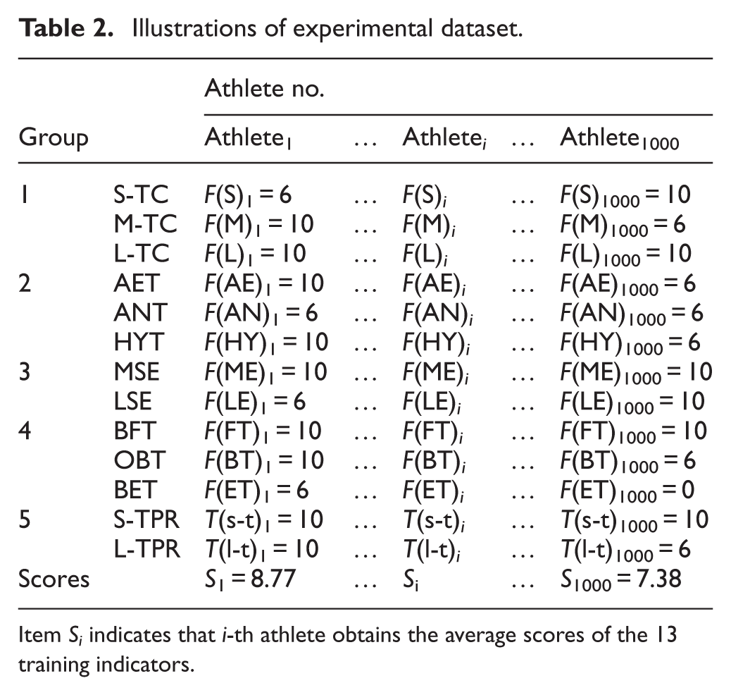
Item S_i indicates that i-th athlete obtains the average scores of the 13 training indicators.

Additionally, we calculated the scores of the 13 indicators in the Group 1–5. The calculated rule is that if each indicator is qualified, athletes can score six points. If each indicator is excellent, athletes can score 10 points. Instead, if each indicator is unqualified, athletes only score 0 points. The average score of i-th athlete within a training cycle is denoted as S_i. Overall, the experimental dataset consists of 1000 rows and 14 columns, meaning that the experimental dataset contains 14,000 data.

Assessment metrics and comparative methods

Precision and F1-score are used for the evaluated metrics to evaluate the forecast ability of our DHNN-WF and the opponents. We chose six competitors Random Forest (RF),⁶ Bayesian method (BM),⁹ Multivariate Regression (MR),¹² Tabular Variational Autoencoders (TVAE),¹⁶ Hidden Markov Model (HMM),¹⁸ and Grey Wolf Optimization based Convolutional Neural Network (GWO-CNN)²⁶ to compare against our DHNN-WF. The seven models (our and the six opponents) were implemented by using Python, and they were run on same TensorFlow experimental environments.

Experimental designs

Experiment (I). Indicator analytic. We analyzed the correlation between the precision of the DHNN-WF and the 13 indicators in Group 1–5 in Table 2. Through calculating their correlation coefficient, the results were analyzed.

Experiment (II). Comparisons on prediction performance. The DHNN-WF was compared against the six opponents RF, BM, MR, TVAE, HMM, and GWO-CNN on the validation set D_val, then compared results were discussed.

Experiment (III). Efficiency. Using the training set D_train to compare the training time of the seven models. Then, the training time was analyzed.

For the six opponents RF, BM, MR, TVAE, HMM, and GWO-CNN, using the same training set D_train to train them, once they were well trained, the same testing set D_test is used for the validation of their parameters. By doing so, this can ensure to have a fair comparison.

Results

This section displays the experimental results, showing that our DHNN-WF outperformed the six competitors in metrics Precision and F1-score, meanwhile, is also a winner in the training efficiency. The details are as follow.

Indicators analytic

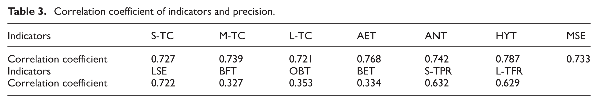
Figure 3 and Table 3 display the correlation coefficient of our precision and the 13 indicators. Through observing the results in Figure 3 and Table 3, there is a weak correlation both the three indicators BFT, OBT, BET in Group 4 and our Precision, that is, the correlation coefficient = 0.327, 0.353, 0.334 and the red bars in Figure 3. However, the rest ten indicators have a strong correlation with our Precision, among which the eight indicators in Group 1–3 (purple bars in Figure 3) show significant correlation with our Precision. These in Figure 3 and Table 3 confirm that the training performance of athletes relies on load structure training, metabolic ability training, skeletal muscle strength training. Hence, we demonstrate that load structure training, metabolic ability training and skeletal muscle strength training are major factors in the improvement of training performance to athletes.

Figure 3.

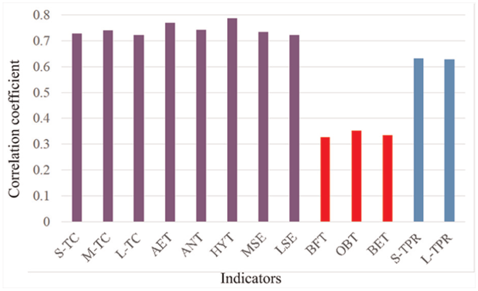
Correlation analytic. Correlation coefficient between the 13 indicators in Group 1–5 and our Precision. The three indicators with the red bars have the low correlation.

Table 3.

Correlation coefficient of indicators and precision.

Indicators	S-TC	M-TC	L-TC	AET	ANT	HYT	MSE
Correlation coefficient	0.727	0.739	0.721	0.768	0.742	0.787	0.733
Indicators	LSE	BFT	OBT	BET	S-TPR	L-TFR
Correlation coefficient	0.722	0.327	0.353	0.334	0.632	0.629

Comparisons on forecast performance

Now, this section begins to compare our DHNN-WF against the six competitors RF, BM, MR, TVAE, HMM, and GWO-CNN in forecast training performance through using the validation set D_val, as shown in Table 4. It can be seen that our DHNN-WF defeated the six competitors in metrics Accuracy, Precision, and F1-score at 95% confidence level. This means that our method predicts the training performance of athletes better than the six competitors do. Whereas, the opponent BM obtains the poorest forecast performance. Additionally, we find that the four models based on neural network architectures DHNN-WF, TVAE, HMM, and GWO-CNN outperform the three machine learning models RF, BM, MR. This imply that these methods based on deep architectures have more advantages than those based on non-deep architectures in the forecast of training performance to athletes.

Table 4.

Comparisons on forecast performance.

Methods	DHNN-WF	MR	RF	TVAE	BM	HMM	GWO-CNN
Accuracy	0.977	0.952	0.956	0.961	0.923	0.933	0.967
Precision	0.971	0.912	0.907	0.922	0.893	0.935	0.951
F1-score	0.912	0.851	0.858	0.866	0.846	0.871	0.882
p = 0.05	*	*	*	*	*	*	*

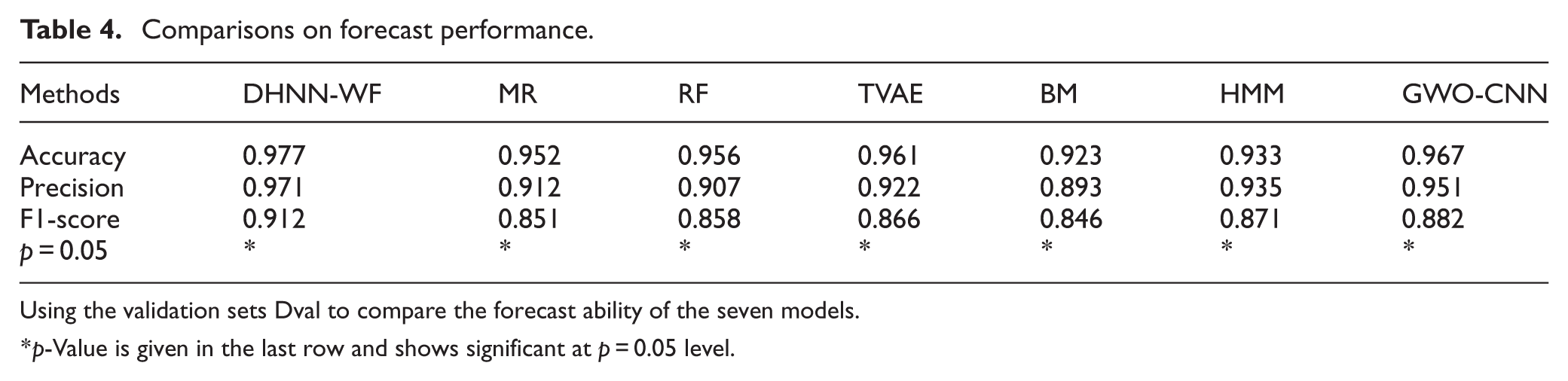
Using the validation sets Dval to compare the forecast ability of the seven models.

p-Value is given in the last row and shows significant at p = 0.05 level.

Table 5 shows the error between the training performance forecasted by the seven models and the real performance obtained from athletes. Our DHNN-WF obtains the minimum error at 95% confidence level. These compared results confirm that the proposed method has ability to forecast the training performance of athletes. Then, according to the forecasted training performance, coaches can design proper training plans for athletes.

Table 5.

Scoring errors.

Methods	DHNN-WF	MR	RF	TVAE	BM	HMM	GWO-CNN
Training	0.0218	0.0779	0.0866	0.0693	0.0953	0.0661	0.0627
Validation	0.0833	0.1222	0.1162	0.1087	0.1323	0.1023	0.1011
p = 0.05	*	*	*	*	*	*	*

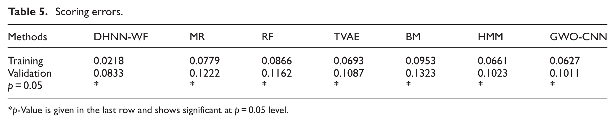
p-Value is given in the last row and shows significant at p = 0.05 level.

Figure 4 displays the error of 10-cross validations of our DHNN-WF. In the 10-cross validations, where 7-cross validations errors of our DHNN-WF remain unchanged, that is, 1–3, 5, 7–9-cross validation, moreover, our DHNN-WF obtains the smallest error in the 7-cross validations. The 10-cross validation results imply that the experimental results obtained by the DHNN-WF is the robustness.

Figure 4.

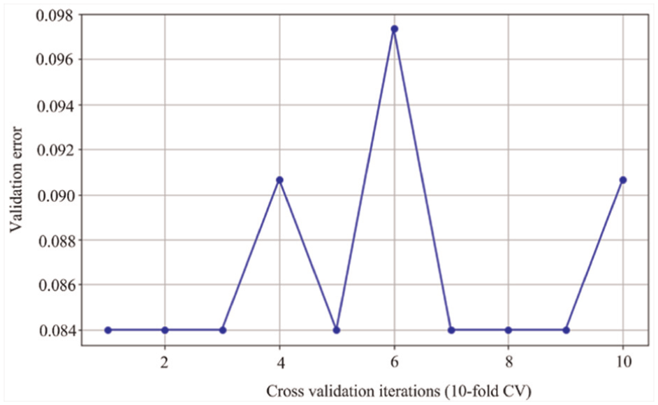
Ten-cross validations of DHNN-WF.

Efficiency

The computational efficiency of all seven models was rigorously evaluated by measuring their training time consumption on the identical training set D_train. As quantitatively summarized in Table 6, our DHNN-WF demonstrated competitive training efficiency relative to benchmark models. While RF and HMM exhibited faster training times (with RF reducing training duration by 16.51 s and HMM by 0.17 s versus DHNN-WF, as per Table 6 data), DHNN-WF achieved significant speed advantages over the four competitors BM, MR, and TVAE, GWO-CNN.

Table 6.

Training time of the seven models.

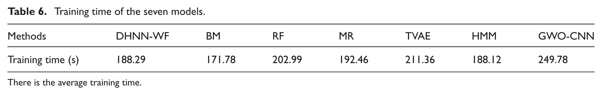
Methods	DHNN-WF	BM	RF	MR	TVAE	HMM	GWO-CNN
Training time (s)	188.29	171.78	202.99	192.46	211.36	188.12	249.78

There is the average training time.

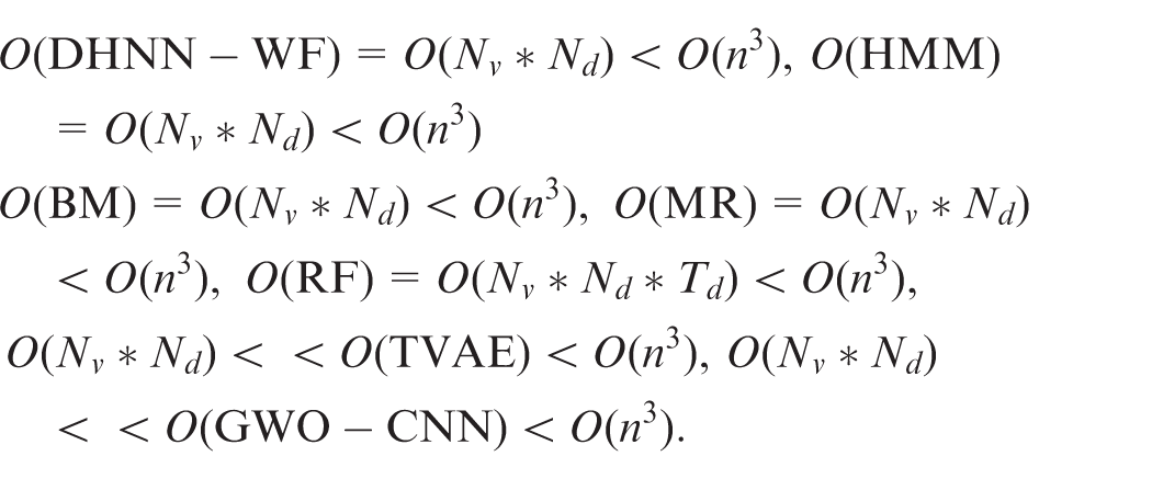
To analyze their time cost, assuming that data dimension is $N_{d}$ , and data volume is $N_{v}$ . Our DHNN-WF major time spent in the state update. The time cost that DHNN-WF updates network status is $O (N_{v} * N_{d})$ . The time consumption of the opponent RF (Random Forest) has a direct relation with tree depth $T_{d}$ , therefore, the time cost $O (RF)$ of RF is $O (N_{v} * N_{d} * T_{d})$ . The time cost $O (HMM)$ of the competitor HMM is $O (N_{v} * N_{d})$ . The opponent MR is an optimized multivariate regression, and the time cost $O (MR)$ is $O (N_{v} * N_{d}) < O (RF) < O (n^{3})$ , where $O (n^{3})$ is the time cost of a multiple linear regression. As for the opponent BM (Bayesian method), the major time consumption is $O (N_{v} * N_{d})$ . The competitor TVAE (Tabular Variational Autoencoders) needs to spent time to cope with the data, therefore the time cost of TVAE contains the time of handing data and that of the training for variational autoencoders. Therefore, TVAE obtain the highest time cost, that is, $O (TVAE) > > O (N_{v} * N_{d})$ . The time consumption of the competitor GWO-CNN contains the training time of CNN and the calculation time of GWO, hence, the time $O (GWO - CNN)$ is greater $O (N_{v} * N_{d})$ . As such, the training time consumption of the seven models are as follows,

\begin{matrix} O (DHNN - WF) = O (N_{v} * N_{d}) < O (n^{3}), O (HMM) \\ = O (N_{v} * N_{d}) < O (n^{3}) \\ O (BM) = O (N_{v} * N_{d}) < O (n^{3}), O (MR) = O (N_{v} * N_{d}) \\ < O (n^{3}), O (RF) = O (N_{v} * N_{d} * T_{d}) < O (n^{3}), \\ O (N_{v} * N_{d}) < < O (TVAE) < O (n^{3}), O (N_{v} * N_{d}) \\ < < O (GWO - CNN) < O (n^{3}) . \end{matrix}

Discussion

Advantages

The proposed method defeats against the six competitors in forecast ability. This is because the prediction ability of Elman neural networks. As is well known, neural networks have excellent data prediction capabilities, therefore, we fully leverage this natural advantage of neural networks. However, the prediction to training performance of athletes relies on many training factors, such as training environments, training intensity, and so on. To effectively express the relations training performance between the training factors, the Meyer wavelet function is introduced into the Elman neural networks. Using the Meyer wavelet function to periodically control the weights of neurons while keeping them in an activated or deactivated state periodically. By doing so, our discrete Elman neural network is promoted in the forecast ability. As a result, that is why the proposed method outperforms the competitors.

Limitations

Firstly, the type of neural networks with Elman structures easily traps a risk of local optimal solutions, compared with other neural network structures. Although our Elman neural network reduces the risk through introducing the Meyer wavelet function to control neurons in activated or deactivated state periodically, our model obtains local optimal solutions with a small probability. But, please note that our model has a certain probability of learning local optimal solutions, nevertheless, this does not imply that our model cannot learn global optimal solutions. Compared with the probability of learning local optimal solutions, that of learning global optimal solutions is greater. Secondly, using equation (7) to update network parameters, the generalization ability of our model may be affected to some extent. Since the update of network parameters depends on the threshold T_j in equation (7), and the calculation of the threshold T_j is periodic.

Additionally, the experimental dataset consists of 1000 rows and 14 columns, implying that the experimental dataset is a low-dimensional dataset, that is, just 14-dimensions. Indeed, the Meyer wavelet function can work well on low-dimensional space, but unfortunately, it is difficulty to be suitable for high-dimensional space due to the curse of dimension. Currently, our model performs well upon low-dimensional space, in future, we need to put into our model on high-dimensional space to verify the performance.

Insights

To integrate the DHNN-WF model into real-world educational environments, the following practical considerations should be addressed,

i) Computational Feasibility & Hardware Requirements. The model can be deployed on standard computing infrastructure (e.g., cloud-based servers or edge devices) due to its efficient wavelet-based feature extraction. For real-time applications (e.g., automated grading or adaptive learning systems), lightweight implementations (e.g., using optimized wavelet transforms) can reduce latency.

ii) Integration with Learning Management Systems (LMS). The DHNN-WF model can be embedded into existing LMS platforms (e.g., Moodle, Blackboard) via API-based wrappers, enabling applications such as automated scoring (using wavelet features for semantic analysis).

iii) Personalized feedback generation (leveraging Hopfield network memory for error pattern recognition).

iv) Teacher and Student Usability. A user-friendly dashboard can visualize wavelet-extracted features (e.g., highlighting areas of improvement in student submissions). Incremental learning can be implemented, allowing the model to adapt to new educational content without full retraining.

While the DHNN-WF model shows theoretical promise, its real-world efficacy depends on seamless integration with existing ed-tech infrastructure, computational optimization, and rigorous empirical validation in classroom settings.

Conclusion

In this work, we used the Event-group training theory to construct 13 training indicators. Then, according to the constructed training indicators, the discrete Hopfield neural network fused with wavelet function is proposed for the training of athletes. Firstly, the 13 training indicators constructed by Event-group training theory are used to calculate training scores of athletes. Thereafter, through calculating the correlation between the 13 training indicators and the training performance predicted by the proposed model, the major training indicators are chosen from the 13 training indicators. Finally, the experimental results show that the proposed model outperformed the competitors in forecast precision of training performance. Results also show that the running efficiency of the proposed model won major competitors. Hence, the constructed 13 training indicators can effectively promote the training of athletes. Through accurately forecasting training performance of athletes, coaches can reasonably propose training plans.

In future work, we will popularize the training plans based on the 13 training indicators to the construction of university physical education courses, thereby providing useful suggestions for the construction of university courses. Furthermore, we will augment DHNN-WF's training by incorporating metaheuristic algorithms (such as Simulated Annealing or Genetic Algorithms) to perturb weight updates and escape local minima. This integration leverages the global search capabilities of metaheuristics combined with DHNN-WF's associative memory, potentially enhancing convergence toward superior solutions, especially for non-convex educational data. Prior to wavelet decomposition handling high-dimensional inputs—like student interaction logs or multimodal sensor data—autoencoder-based feature compression is incorporated. Stacked denoising autoencoders learn compact input representations, preserving critical patterns while reducing computational overhead and mitigating dimensionality issues. Finally, DHNN-WF operates within a federated learning framework where localized models (e.g., per-school instances) share exclusively wavelet feature embeddings. This distributed approach maintains data privacy while enabling scalability across multi-institutional datasets.

Footnotes

ORCID iD

Bin Wu

Funding

The authors received no financial support for the research, authorship, and/or publication of this article.

Declaration of conflicting interests

The authors declared no potential conflicts of interest with respect to the research, authorship, and/or publication of this article.

References

Gao

Zhong

. Research on the structural characteristics of sports training system. In: 2010 International conference on system science, engineering design and manufacturing informatization, China, 2010, pp.1–6.

Liu

Zou

. Optimization study of sports training management in perspective of injuries and disabilities: taking Liaoning Province athletes as a case. In: 2012 24th Chinese control and decision conference, China, 2012, pp.1–4. IEEE.

Sawyer

CM.

A survey of team members who participate in traumatic event group psychological debriefings. Indiana University Publishing, 2000.

Zhang

Luo

Optimization algorithm analysis of sports performance influence factors based on radar identification chart. J Simul 2014; 2(5): 255–257.

Liu

Three-dimensional image analysis and discussion on the movement characteristics of cross kick in Taekwondo. J Phys Conf Ser 2021; 1744: 1–5.

Jose

Maliackal

Sukumaran

, et al. Machine learning technique to analyze the health condition of athletes and predict their performance. In: 2023 International conference on circuit power and computing technologies, 2023, pp.1–10. IEEE.

. Application of the artificial intelligence sensor principle in athlete training status testing system. In: 2023 2nd International conference on artificial intelligence and computer information technology, 2023, pp.1–6. IEEE.

Worsey

MTO

Espinosa

Shepherd

, et al. One size doesn’t fit all: supervised machine learning classification in athlete-monitoring. IEEE Sens Lett 2021; 5(3): 1–16.

Zhu

Hong

. Intelligent recognition of incorrect movements in athlete training under artificial intelligence technology. In: 2023 2nd International conference on artificial intelligence and computer information technology, 2023, pp.1–8. IEEE.

10.

Zhao

. Research on scientific training system of track and field athletes based on computer 3D visualization technology. In: 2023 IEEE international conference on sensors, electronics and computer engineering, 2023, pp.1–10. IEEE.

11.

Cao

Zhu

Zhang

, et al. Blockchain-enabled HMM model for sports performance prediction. IEEE Access 2021; 9: 40255–40262.

12.

Murthy

Taetz

Lekhra

, et al. DiveNet: dive action localization and physical pose parameter extraction for high performance training. IEEE Access 2023; 11: 37749–37767.

13.

Juliano

Thakkar

Taber

, et al. A dynamic online dashboard for tracking the performance of division 1 basketball athletic performance. In: 2023 IEEE 28th pacific rim international symposium on dependable computing, 2023, pp.1–13. IEEE.

14.

Alcazar

CJM

Batalla

Figueroa

MJS

, et al. NUPro: a mobile and web framework for athlete profiling and training load monitoring. In: 2021 1st International conference in information and computing research, 2021, pp.1–11. IEEE.

15.

Xianguo

Cong

. Research on the application of artificial intelligence technology in physical training. In: 2021 2nd International conference on big data and informatization education, 2021, pp.1–9. IEEE.

16.

Morciano

Zingoni

Morachioli

, et al. Machine Learning prediction of the expected performance of football player during training. In: 2022 IEEE international conference on metrology for extended reality, artificial intelligence and neural engineering, 2022, pp.1–10. IEEE.

17.

Yuanjun

. Research on the application of computer artificial intelligence technology in improving scientific training performance. In: 2022 International conference on education, network and information technology, 2022, pp.1–13. IEEE.

18.

Qiao

. Research on digital sports training system based on information fusion technology. In: 2023 International conference on power, electrical engineering, electronics and control, 2023, pp.1–10. IEEE.

19.

Meng

Yang

Huang

. Intervention of football players’ training effect based on machine learning. In: 2022 2nd International conference on consumer electronics and computer engineering, 2022, pp.1–5. IEEE.

20.

Yahyasoltani

Annapureddy

Farazi

Learning performance efficiency of college basketball players using TVAE. IEEE Access 2023; 11: 130186–130196.

21.

Szmygin

Wojtowicz

Chadaj

, et al. Prediction of athletes’ performance results using machine learning algorithms. In: 2023 24th International conference on computational problems of electrical engineering, 2023, pp.1–9. IEEE.

22.

Biró

Cuesta-Vargas

Szilágyi

. AI-controlled training method for performance hardening or injury recovery in sports. In: 2024 IEEE 22nd world symposium on applied machine intelligence and informatics, 2024, pp.1–6. IEEE.

23.

Gupta

Naveen

Sukumar

, et al. Hyperbolic hopfield neural network for enhanced solar power generation forecasting. In: 2024 4th International conference on mobile networks and wireless communications (ICMNWC), 2024, pp.1–6.

24.

Betteti

Baggio

Zampieri

. On the capacity of continuous-time Hopfield models. In: 2024 IEEE 63rd conference on decision and control (CDC), Milan, Italy, 2024, pp.7853–7858.

25.

Yue-Yang

, et al. Continuous self-learning control under system identification based on Hopfield neural network. In: 2024 China automation congress (CAC), 2024, pp.2554–2560.

26.

Wang

Huang

. A dynamic analysis of a dual memristive Hopfield neural network. In: 2024 4th International conference on neural networks, information and communication engineering (NNICE), 2024, pp.114–119.

27.

Almogahed

Mahdin

, et al. Multi-classification refactoring framework using Hopfield neural network for sustainable software development. IEEE Access 2025; 13: 31785–31808.

28.

Zhang

Chen

Zhang

, et al. Multidirectional Multidouble-Scroll Hopfield Neural Network with application to image encryption. IEEE Trans Syst Man Cybern Syst 2025; 55(1): 735–774.

29.

Peng

Zeng

, et al. Adjusting dynamics of Hopfield Neural Network via time-variant stimulus. IEEE Trans Circuits Syst 2024; 71(7): 3242–3255.

30.

Zhu

Peng

Zhang

, et al. Generation power prediction method of distributed new energy system based on Wavelet Neural Network. In: 2024 4th International conference on smart grid and energy internet (SGEI), 2024, pp.26–31.

31.

Gao

Wang

. An online milling surface roughness prediction method for thin-walled blade based on wavelet transform and convolutional neural network integrated with a digital twin system. In: 2024 5th International seminar on artificial intelligence, networking and information technology (AINIT), 2024, pp.889–896.

32.

Wang

Yang

Nie

, et al. LSTM vibration prediction based on wavelet analysis and pso for the pumped storage hydropower unit. In: 2024 14th International conference on power and energy systems (ICPES), 2024, pp.492–498.

33.

Dai

Yuan

Tian

, et al. A novel wavelet based generative model for time series prediction. In: 2024 10th International conference on big data and information analytics (BigDIA), 2024, pp.178–182.

34.

Shukla

Gupta

Pasari

, et al. Wind speed prediction using empirical wavelet transform and bidirectional gated recurrent unit based hybrid model. In: 2024 15th International conference on computing communication and networking technologies (ICCCNT), 2024, pp.1–5.

35.

Habelalmateen

Palanivel

Bharattej

RRVSS

, et al. Wavelet transform based bidirectional long short-term memory for predicting water demand. In: 2024 First international conference on software, systems and information technology (SSITCON), 2024, pp.1–4.

Athlete performance prediction using discrete neural networks based on Event-group training theory

Abstract

Keywords

Introduction

Motivation

Contributions

Related works

Methods

Overall scheme

Training indicators based on event-group training theory

Model design

Model structure

Wavelet function

Parameter configuration

Model training

Experimental settings

Datasets

Assessment metrics and comparative methods

Experimental designs

Results

Indicators analytic

Comparisons on forecast performance

Efficiency

Discussion

Advantages

Limitations

Insights

Conclusion

Footnotes

ORCID iD

Funding

Declaration of conflicting interests

References