Sage Journals: Discover world-class research

Abstract

The precise measurement of pulsed signals, especially fast/broadband pulsed signals, has always been a research topic of concern. Broadband sampling oscilloscopes are the most effective electronic instruments for measuring pulsed signals. In the precise measurement of such signals, the time-base jitter of broadband sampling oscilloscopes is a key factor affecting accuracy. This paper employs the orthogonal distance regression algorithm based on a three-channel synchronous measurement system to estimate the time-base jitter of the sampling oscilloscope and realizes its compensation through a linear interpolation algorithm. Meanwhile, the jitter value and Type A uncertainty of the pulsed signal itself are measured to evaluate the compensation effect. The results demonstrate that when the measured signal is a pulse, the three-channel synchronous measurement system and the proposed algorithm can effectively compensate for the time-base jitter of the sampling oscilloscope, providing an efficient solution for precise pulsed signal measurement.

Keywords

time-base jitter orthogonal distance regression algorithm pulse signal jitter compensation broadband sampling oscilloscope

Introduction

In the field of modern electronic measurement, the broadband sampling oscilloscope, as a key time-domain measurement instrument, has its measurement accuracy significantly affected by time-base jitter, which impairs the accurate evaluation of signal parameters. Time-base jitter is an important parameter characterizing signal and system performance.¹ For sampling oscilloscopes, since sampling points deviate from their ideal time positions, random errors occur in sampled values; this type of time-base jitter is also referred to as “jitter measurement floor” in some literatures. Due to the existence of jitter measurement floor, when a sampling oscilloscope is used to measure signals, the jitter value in the measurement results includes both the time-base jitter of the measured signal and the jitter measurement floor of the oscilloscope itself. Consequently, the measurement results may mislead the judgment of the signal’s true characteristics and lead to large errors. To ensure higher accuracy of measurement results, it is crucial to eliminate or mitigate the impact of the oscilloscope’s time-base jitter on the results.

In this paper, the Orthogonal Distance Regression (ODR) algorithm is adopted, with an orthogonal sinusoidal signal as the reference signal, which can effectively estimate and compensate for the time-base jitter of the sampling oscilloscope. Currently, this algorithm has demonstrated excellent performance when the measured signal is a sinusoidal signal,² but its applicability to pulse signals remains to be verified.

As is well-known, among all signals, pulse signals are the most difficult to measure, occupy the widest frequency band, have the richest frequency components, and possess the highest theoretical research value. However, research on the accurate measurement of pulse signals is relatively scarce. Even a tiny time offset can cause the pulse amplitude measurement error to exceed 10%, and the transition edge time deviation can reach the order of hundreds of picoseconds. Therefore, eliminating or compensating for the interference of time-base jitter on pulse signal measurement is a key issue for improving the measurement performance of broadband sampling oscilloscopes.

Complete elimination of an oscilloscope’s time-base jitter is impractical; currently, only maximum compensation can be achieved, which is mainly divided into two approaches: hardware optimization and algorithmic calibration. Hardware-level methods, which are not elaborated here, include but are not limited to phase-locked loop technology and ultra-low noise crystal oscillators. However, they suffer from a critical drawback: hardware optimization is technically challenging, and improvement is particularly difficult in high-frequency measurement fields. In terms of algorithms, early methods mostly relied on Fourier transform, using the signal’s frequency spectrum to compensate for the oscilloscope’s time-base jitter, but their adaptability to pulse signals is poor. The Kalman filtering algorithm depends on an accurate jitter model and lacks flexibility in complex environments. In recent years, the ODR algorithm has emerged as the most effective approach—it can simultaneously optimize errors in both time-base jitter and amplitude. While its effectiveness has been verified in jitter compensation for sinusoidal signals, its application to non-periodic, transient signals such as pulse signals remains unknown.

Aiming at the aforementioned problems and focusing on the accurate measurement of pulse signals, this study for the first time extends the ODR algorithm to the time-base jitter compensation of pulse signals, systematically investigates the practicality of this scheme, and breaks through the limitation of the algorithm’s application to periodic signals. In this paper, a three-channel synchronous measurement system with pulse signals as the measured objects is used. The ODR algorithm and interpolation algorithm are applied to estimate and compensate for the time-base jitter of the sampling oscilloscope in the measured pulse waveforms. Finally, the compensation effect of the sampling oscilloscope’s time-base jitter is evaluated by comparing the jitter value changes of the pulse waveform data before and after compensation, as well as through the evaluation of waveform measurement uncertainty.

Influence of time-base jitter in broadband sampling oscilloscopes on signal measurement

The time-base jitter of broadband sampling oscilloscopes essentially stems from inaccurate amplitude sampling caused by deviations in sampling time. This is because the sampling pulses are derived from a clock, which in turn originates from a crystal oscillator—a device with limited frequency stability and accuracy. The sampling pulses are generated through circuits connected to the crystal oscillator, and due to the imperfections in these circuits, the actual sampling moments deviate from the ideal ones, forming errors. Specifically, the sampling process of an oscilloscope relies on the coordinated operation of a trigger signal and an internal clock. The trigger signal ensures synchronization at the same phase point of each cycle for periodic signals, while the internal clock controls the timing of sampling intervals. Under ideal conditions, the sequential equivalent sampling mode would acquire signals at strictly equidistant time points, as shown in Figure 1. However, due to actual clock jitter and the influence of multiple factors such as thermal noise in the oscilloscope, the sampling moments deviate from their theoretical positions, leading to uneven sampling intervals and causing time-base jitter. The time-base jitter of sampling oscilloscopes can distort the time-domain waveform of signals and introduce phase noise in the frequency domain, directly affecting the measurement accuracy of the oscilloscope. Therefore, clock jitter manifests as the temporal uncertainty of the sampling clock edges, while the stability of the trigger signal determines the synchronization accuracy of the sampling start point. Together, they determine the timing accuracy of the sampling process.³

Figure 1.

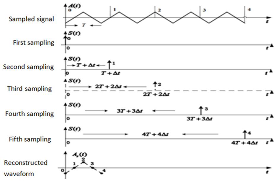
Schematic diagram of sequential equivalent sampling.

In the accessible literature, the time-base jitter problem of oscilloscopes has been estimated and evaluated using sinusoidal signals,^4,5 which has a complete theoretical foundation. This is because the mathematical description of sinusoidal signals is simple and clear, their time-domain and frequency-domain characteristics can be strictly corresponded through Fourier transform, and the measurement of continuous waveform signals by various measuring devices is relatively convenient. The following simulates the sampling process of multiple groups of sinusoidal signals through a sampling oscilloscope and shows the waveforms affected by the time-base jitter of the sampling oscilloscope. Here, only the unilateral spectrum is plotted, as shown in Figure 2. In the time domain, time-base jitter causes deviation from the ideal position during sampling, resulting in amplitude errors in sampling and making the waveform contour “thicker.” In the frequency domain, it forms phase noise and increases frequency components.

Figure 2.

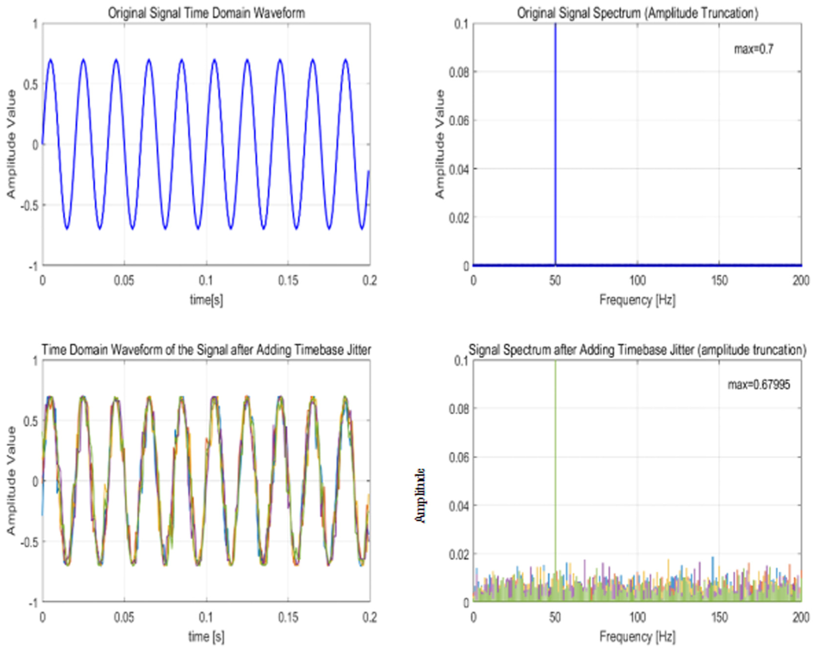
Comparison diagram of waveforms affected by time-base jitter.

Jitter of pulse signals and calculation methods

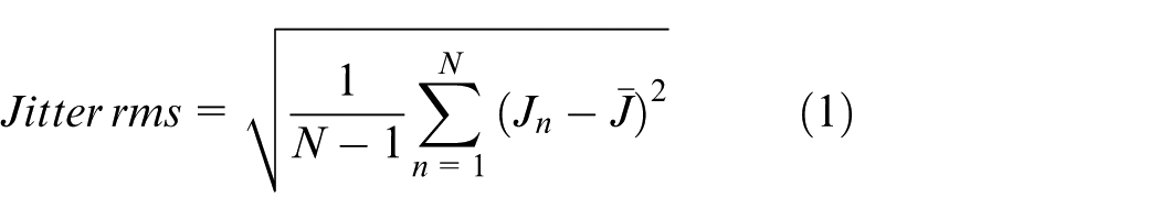
For a broadband system, narrowband signals are difficult to fully excite its system characteristics. Therefore, in this paper, pulse waveforms are selected to estimate and compensate the jitter measurement floor of the oscilloscope, which is more theoretically valuable and practical for the precise measurement of broadband signals. Since the time-base jitter of the signal is random, the root mean square (RMS) is usually used to evaluate the statistical distribution characteristics after overlapping multiple waveforms, which complies with the regulations in IEC 60469 and IEEE 2414-2020,^6,7 as shown in equation (1). In equation (1), N refers to the number of collectible points within the window, called sample points; $J_{n}$ refers to the moment corresponding to the sample point; and $\bar{J}$ is the average value of all sample points.

Jitter rms = \sqrt{\frac{1}{N - 1} \sum_{n = 1}^{N} {(J_{n} - \bar{J})}^{2}}

(1)

Keysight Technologies’ test solution⁷ involves setting a window with a 5% amplitude range centered around the amplitude median. After overlaying multiple acquired waveforms, the time instants corresponding to all sampling points falling within this window are collected to compute the signal’s jitter value. Figure 3 illustrates the jitter measurement process for a pulse signal in FlexDCA simulation, along with a histogram of the signal’s time-base jitter, validating the random nature of the jitter.⁹

Figure 3.

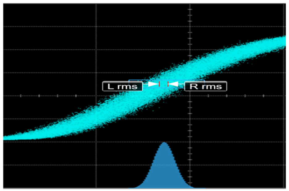
Time-base jitter measurement method for pulse signals.

Compensation for time-base jitter in sampling oscilloscopes using orthogonal distance regression and linear interpolation algorithms

The Orthogonal Distance Regression (ODR) algorithm is a highly effective method for estimating the time-base jitter of sampling oscilloscopes.^4,10 This approach can accurately estimate the time-base errors of sampling oscilloscopes by using a set of orthogonal sinusoidal signals. The algorithm is optimized based on the least squares method and can simultaneously estimate errors in two directions. References 1 and 4 verify the measurement of sinusoidal signals by this algorithm under different conditions, indicating that it can effectively estimate the jitter measurement floor of oscilloscopes.

The objective function is the key to this algorithm, which is defined as the sum of squares of the orthogonal distances from the sampling points to the model.

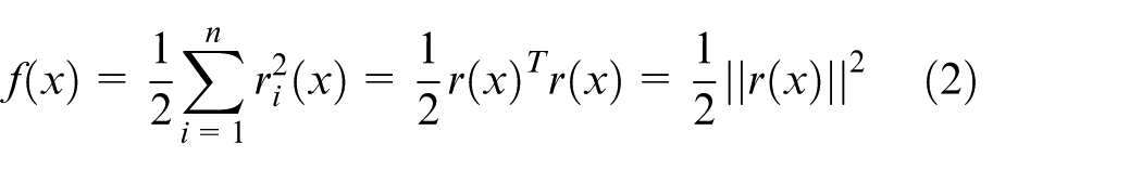
f (x) = \frac{1}{2} \sum_{i = 1}^{n} r_{i}^{2} (x) = \frac{1}{2} r {(x)}^{T} r (x) = \frac{1}{2} {| | r (x) | |}^{2}

(2)

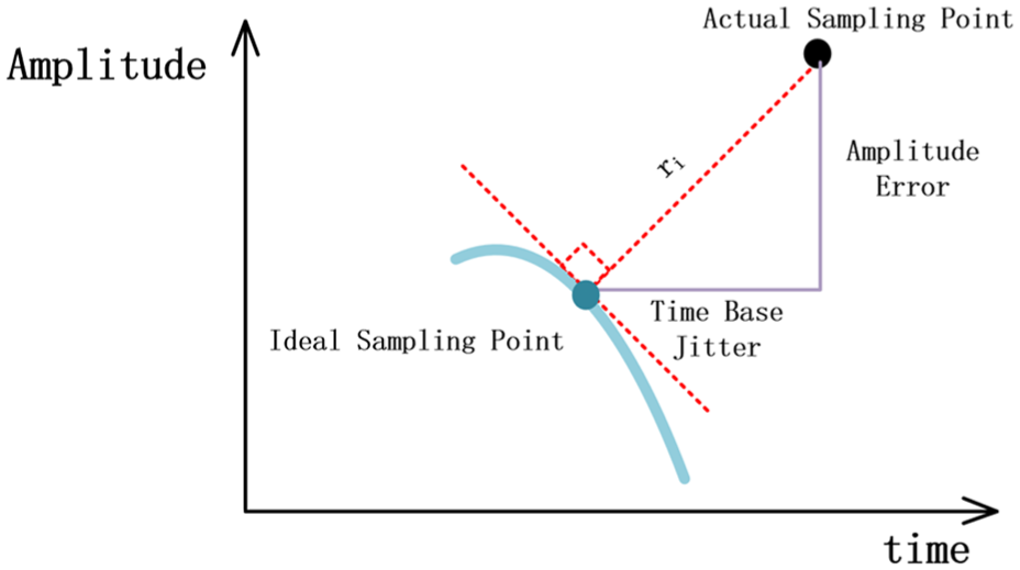
In equation (2), $r_{I}$ is the residual of the $i$ point, and $| | r (x) | |$ represents the 2-norm. Mathematically, the 2-norm can be interpreted as the orthogonal distance. As shown in Figure 4, ODR can simultaneously estimate both the time-base jitter and amplitude errors (which can be regarded as vertical jitter), thereby improving the accuracy and stability of jitter estimation.

Figure 4.

Orthogonal distance from sampling points to ideal sampling points.

This paper uses a set of orthogonal sinusoidal signals as reference signals, and estimates the time-base jitter of broadband sampling oscilloscopes through an orthogonal distance regression algorithm. The algorithm model of the reference signals is expressed as follows⁴:

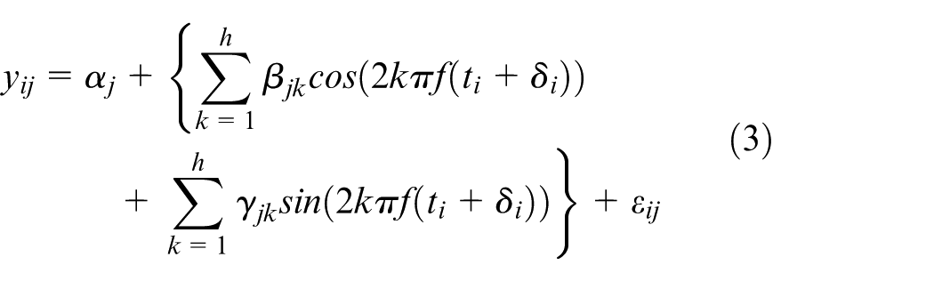
\begin{matrix} y_{ij} = α_{j} + {\sum_{k = 1}^{h} β_{jk} \cos (2 k π f (t_{i} + δ_{i})) \end{matrix} + \sum_{k = 1}^{h} γ_{jk} \sin (2 k π f (t_{i} + δ_{i}))} + ε_{ij}

(3)

In equation (3), $y_{ij}$ is the sampled amplitude value of the $i^{th}$ channel’s reference sinusoidal signal at the $j^{th}$ sampling point; $f$ is the frequency of a set of approximately orthogonal reference sinusoidal signals; $h$ is the harmonic number, typically taking the value of 3,² $β_{jk}$ and $γ_{jk}$ are respectively the amplitudes of the $h^{th}$ harmonic of the $i^{th}$ orthogonal reference signal; $t_{i}$ is the $i^{th}$ ideal sampling time; $ε_{ij}$ represents the amplitude error caused by noise; and $δ_{i}$ denotes the time-base jitter at the $i^{th}$ sampling time. The calculation of the residual is performed through the orthogonal distance between the actual sampling points and the ideal sampling points.

Parameter optimization is performed through iteration: Fix the time-base jitter, solve the linear least squares problem, and update the waveform parameters $α_{j}, β_{jk}$ and $γ_{jk}$ ; fix the waveform parameters and optimize $δ_{i}$ using the trust-region algorithm.

In simple terms, the initial jitter value is first used to estimate and correct the waveform shape, and then the corrected waveform is used to back-calculate a more accurate jitter value. Typically, the initial $δ_{i}$ in the first iteration is 0, and subsequent iterations aim to minimize the residual (i.e. find the corresponding orthogonal distance), translate the reference signal model, and determine the precise oscilloscope jitter measurement floor.

The advantage of this iteration lies in improving computational efficiency by separating linear and nonlinear steps, and ensuring the objective function decreases monotonically through dynamic adjustment of the step size.⁵

Having briefly introduced the process of the ODR algorithm above, the detailed process is shown in Figure 5.

Figure 5.

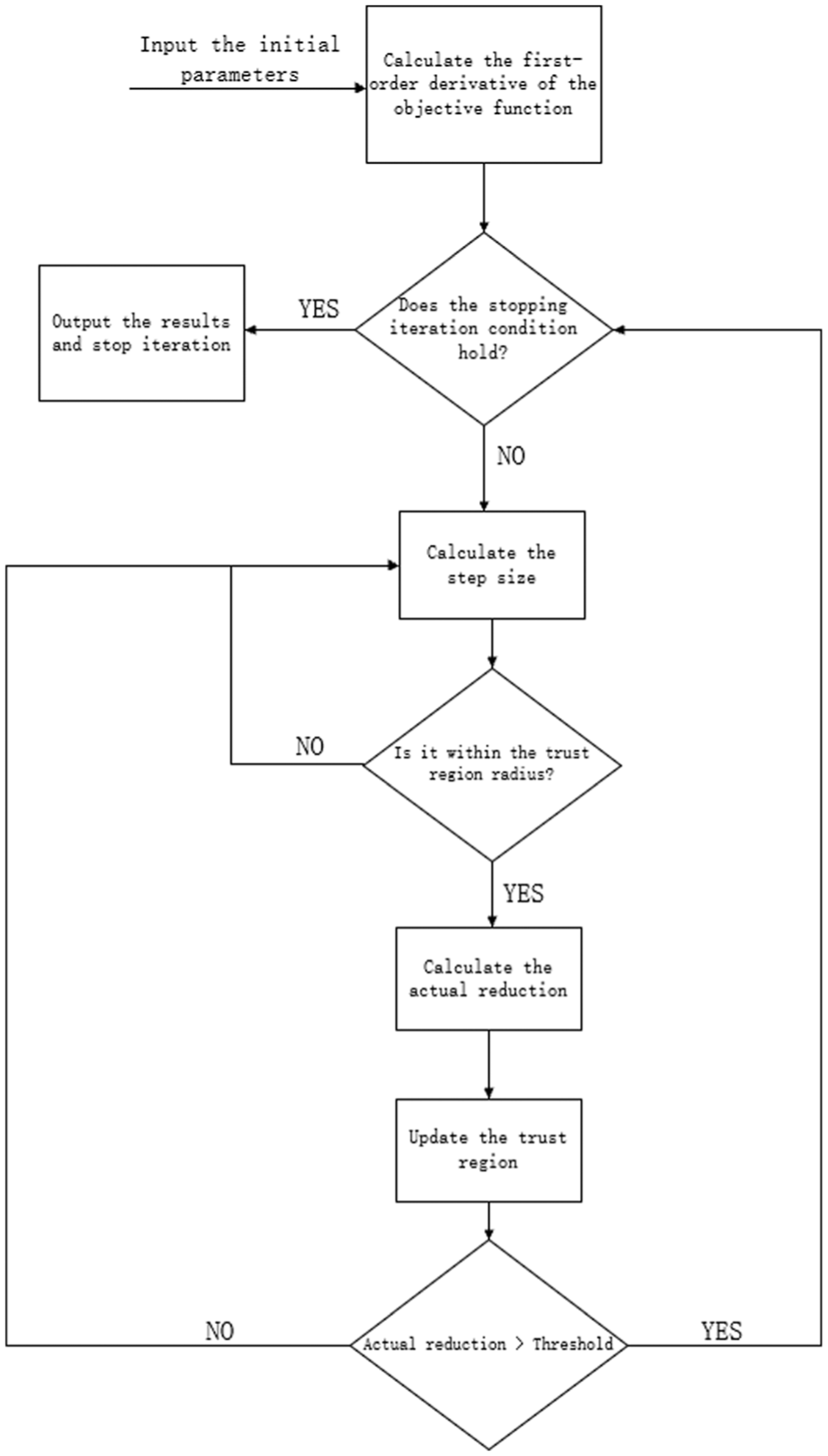
Flow chart of the ODR algorithm.

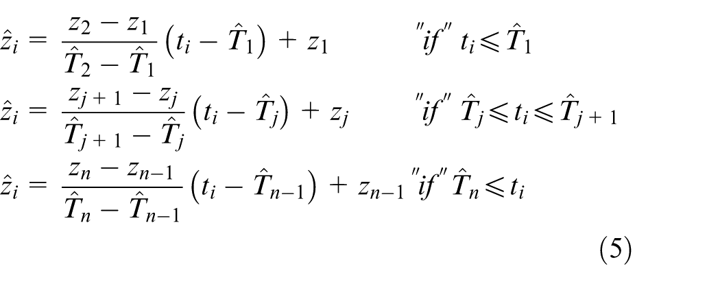
After estimating the jitter using the orthogonal distance regression algorithm, the linear interpolation algorithm is combined to compensate the estimated jitter into the acquired waveform data. The key is to remap the non-uniform sampling data caused by the time-base jitter of the sampling oscilloscope to the ideal sampling time, which effectively compensates for the influence of the time-base jitter of the sampling oscilloscope on the measured signal.

Based on the equivalent time sampling principle of the broadband sampling oscilloscope, assuming the ideal sampling time is $T_{s}$ and the estimated value of the time-base jitter is $δ_{i}$ , the actual sampling time of each point is obtained through equation (4):

t_{i} = (i - 1) T_{s} + δ_{i}

(4)

After sorting the actual sampling points by time and reconfiguring the sampling values according to equation (4), linear interpolation is performed on the non-uniform sampling data caused by time-base jitter using equation (5).⁸ In equation (5), $z_{j}$ represents the measured value of the $j^{th}$ known point, ${\hat{T}}_{j}$ is the time point excluding the time-base jitter of the sampling oscilloscope, $t_{i}$ is the ideal time point, ${\hat{z}}_{i}$ is the estimated value of the ideal time point, and $n$ is the total number of data points. By remapping these to the ideal sampling time, the values on both sides of the endpoints are also estimated, thus completing the compensation for time-base jitter.

\begin{matrix} {\hat{z}}_{i} = \frac{z_{2} - z_{1}}{{\hat{T}}_{2} - {\hat{T}}_{1}} (t_{i} - {\hat{T}}_{1}) + z_{1} if t_{i} \leq {\hat{T}}_{1} \\ {\hat{z}}_{i} = \frac{z_{j + 1} - z_{j}}{{\hat{T}}_{j + 1} - {\hat{T}}_{j}} (t_{i} - {\hat{T}}_{j}) + z_{j} if {\hat{T}}_{j} \leq t_{i} \leq {\hat{T}}_{j + 1} \\ {\hat{z}}_{i} = \frac{z_{n} - z_{n - 1}}{{\hat{T}}_{n} - {\hat{T}}_{n - 1}} (t_{i} - {\hat{T}}_{n - 1}) + z_{n - 1} if {\hat{T}}_{n} \leq t_{i} \end{matrix}

(5)

Having now introduced all algorithmic processes in full, the overall application flow is shown in Figure 6.

Figure 6.

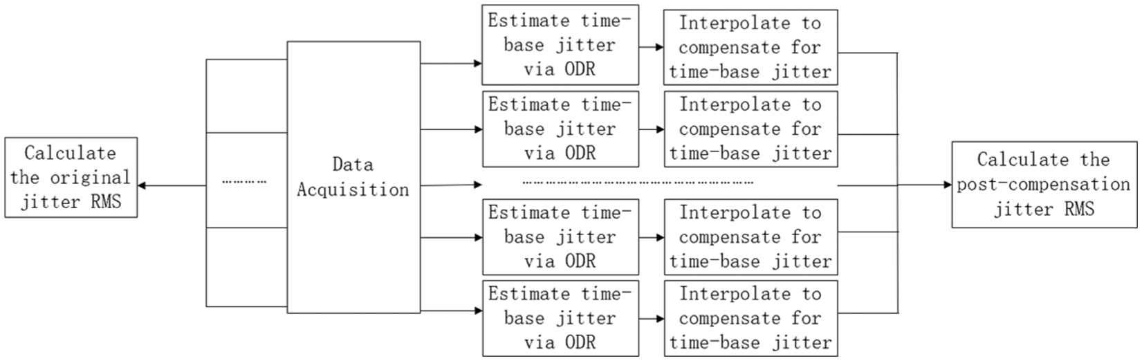
Application flow chart of the algorithm in this paper.

Construction of three-channel synchronous measurement system

To accurately estimate the time-base jitter of the sampling oscilloscope and compensate it in the pulse signal waveform, a three-channel synchronous measurement system was constructed based on the orthogonal distance regression algorithm. A set of orthogonal sinusoidal signals are input into the first two channels to estimate the jitter measurement floor of the oscilloscope, and the estimated jitter is compensated into the measured signal in the third channel. As previously mentioned, the jitter measured by the oscilloscope includes the comprehensive influence of the signal source, oscilloscope, and other instruments. Therefore, a low-jitter signal source was selected to generate sinusoidal signals when constructing the measurement system, so that the estimation result can be approximately regarded as the jitter measurement floor of the oscilloscope, that is, the time-base jitter of the sampling oscilloscope. An orthogonal coupler is used to realize the orthogonality of the sinusoidal signals, and a fast edge generator differentiates the sinusoidal signals into pulse signals,¹¹ where the frequency of the sinusoidal signals is the fundamental frequency of the pulse signals. It is generally assumed that the internal channel jitters of the oscilloscope are the same and the entire system is synchronized, allowing the orthogonal distance regression algorithm to estimate the jitter and compensate it into the pulse signals. The connection block diagram is shown in Figure 7.

Figure 7.

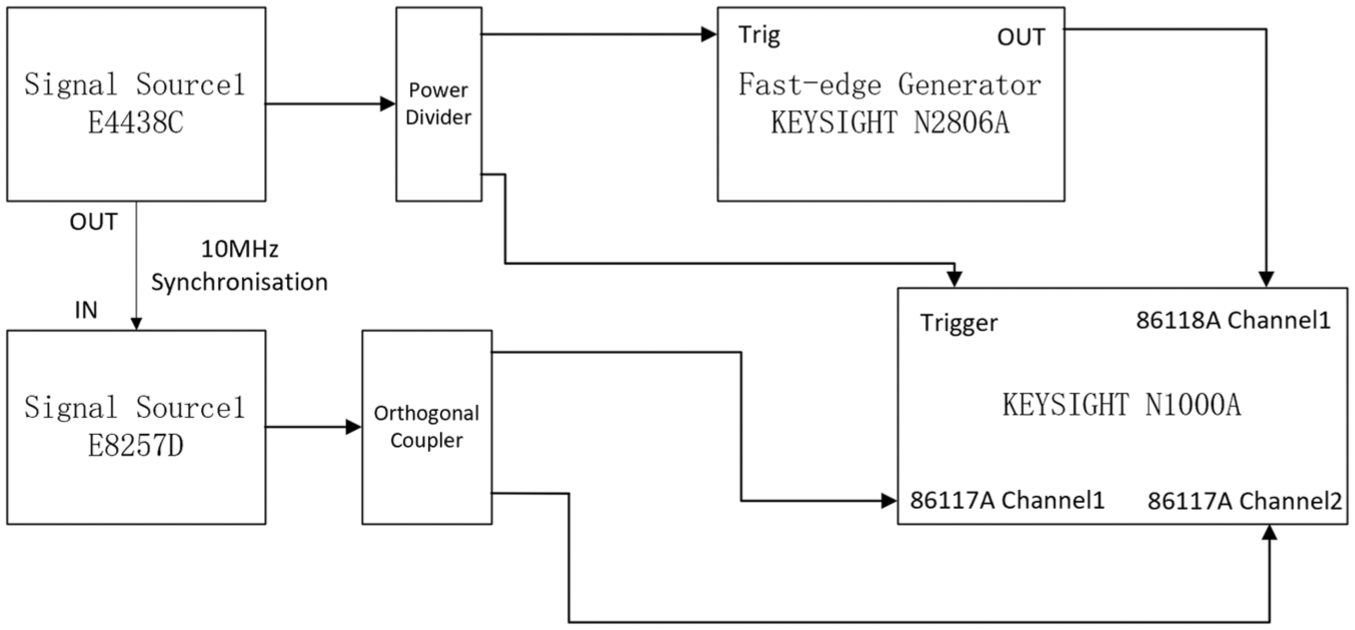
Connection diagram of the measurement system.

During the measurement, the following points need attention:

Verify the performance of the orthogonal coupler in advance using a vector network analyzer. In this study, the orthogonal coupler has been verified to perform well, satisfying orthogonality within the range of 2G–18G.

Ensure synchronization of the entire system. Two low-jitter signal sources are connected via coaxial cables, and the sinusoidal signal generating the pulse signal is input into the oscilloscope’s external trigger port to serve as the trigger signal. This connection ensures the synchronization of the entire measurement system and improves measurement accuracy.

Guarantee the integrity of the acquired signals. This paper focuses on the applicability of the orthogonal regression algorithm for pulsed measured signals. Therefore, it is crucial to acquire a pulse signal with complete information and multiple cycles of orthogonal sinusoidal signals. This means the frequency of the sinusoidal signal must maintain an integer multiple relationship with the fundamental frequency (i.e. the repetition frequency) of the pulse signal. This ensures that while a complete cycle of the pulse signal is acquired, multiple cycles of the sinusoidal signal are also captured. Additionally, using a sinusoidal signal with a lower frequency as the oscilloscope’s external trigger can enhance trigger stability and reduce extra errors introduced by triggering.

Through the above connection method, it is ensured that the pulse waveform is completely sampled in the time domain, and the data collected by the synchronous system meets the conditions for applying the orthogonal distance regression algorithm, providing reliable data support for subsequent compensation of the pulse waveform. The actual connection diagram of the measurement system is shown in Figure 8, and the data collected by the oscilloscope through this system is shown in Figure 9.

Figure 8.

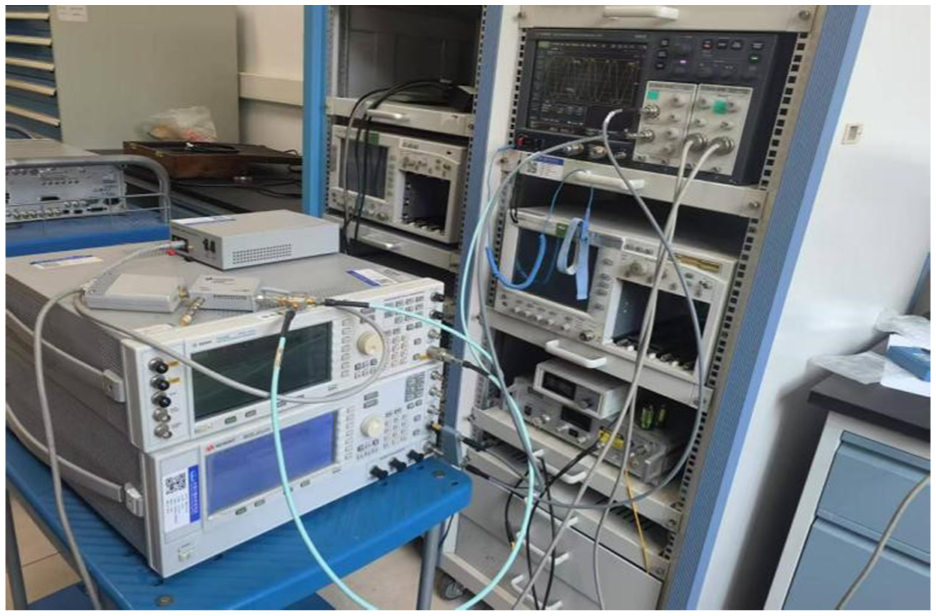
Actual connection diagram of the synchronous measurement system.

Figure 9.

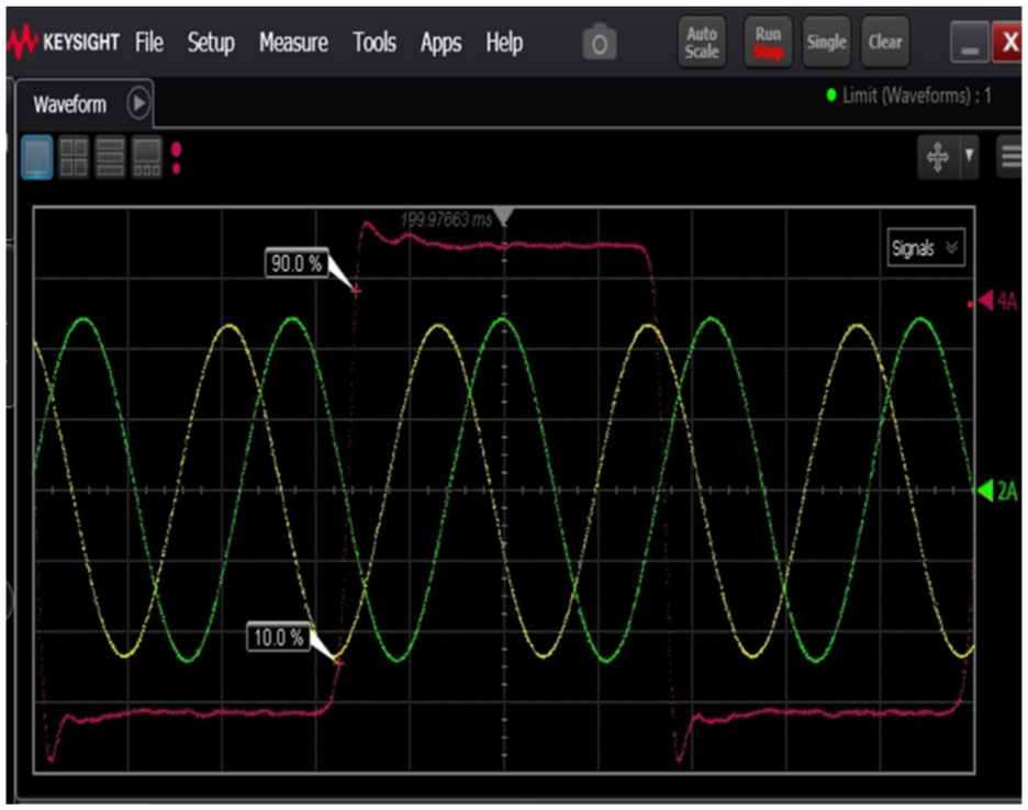
Waveforms acquired by the oscilloscope.

Data processing

Time-base jitter of pulse signals

In this experiment, the original single waveform collected is shown in Figure 8. A total of 70 groups of waveforms were collected for calculation, with the fundamental frequency of the pulse signal being 3G and the frequency of the orthogonal sinusoidal signal being 9G, denoted as 3G–9G, as shown in Figure 10.

Figure 10.

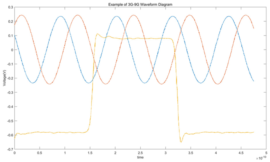
Example of 3G–9G waveform diagram.

Figure 11 shows the overall effect of the 70 groups of signals and plots the 5% region in the central area of the figure. By calculating the 5% of the central area of the rising edge, the jitter of the signal is calculated to be 413fs. It can be seen that the cumulative waveform lines of the 70 groups of waveforms are “thicker,” reflecting the influence of the time-base jitter of the sampling oscilloscope on the measured signal.

Figure 11.

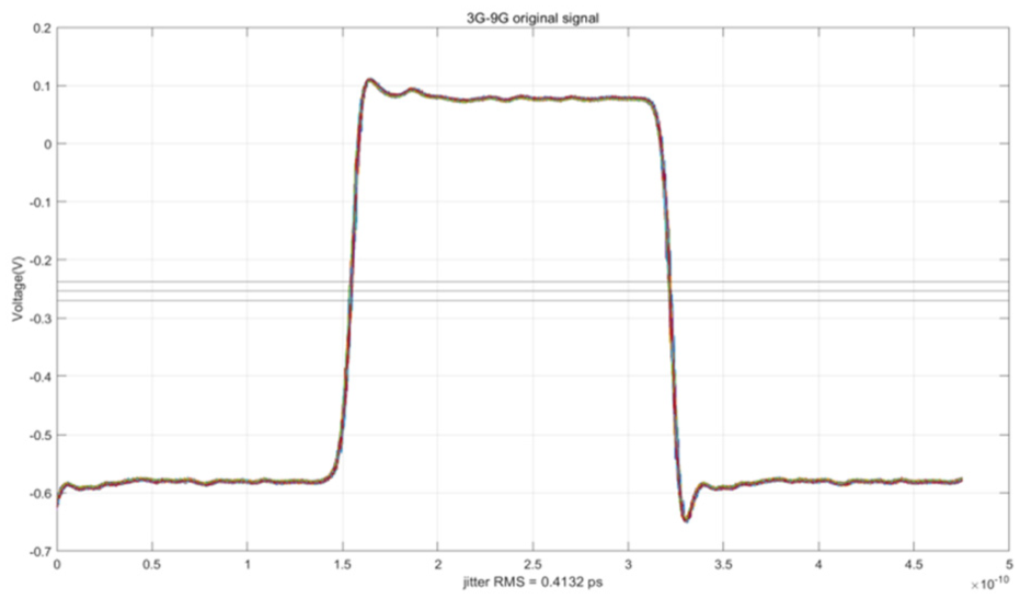
Original waveforms of the 3G–9G group.

The time-base jitter of the sampling oscilloscope is estimated by the orthogonal distance regression algorithm, and the jitter is compensated by the linear interpolation algorithm. The compensated 70 sets of waveforms are redrawn as shown in Figure 12. It can be seen that in the rising edge part, most of the amplitude instability phenomenon is suppressed. Moreover, from the perspective of the lines after waveform accumulation, the lines of the compensated waveform are significantly thinner than those of the original waveform, which indicates that the algorithm can effectively compensate for the time-base jitter of the oscilloscope. In terms of data, the jitter after compensation is 255fs, and 38.3% of the jitter is compensated.

Figure 12.

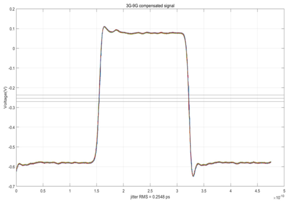
Compensated waveforms of 3G–9G group.

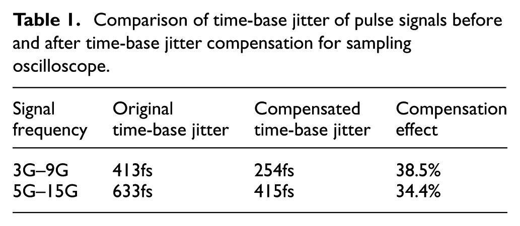
This paper lists and compares the time-base jitter values of the pulse signal before and after time-base jitter compensation for the sampling oscilloscope, as shown in Table 1.

Table 1.

Comparison of time-base jitter of pulse signals before and after time-base jitter compensation for sampling oscilloscope.

Signal frequency	Original time-base jitter	Compensated time-base jitter	Compensation effect
3G–9G	413fs	254fs	38.5%
5G–15G	633fs	415fs	34.4%

Evaluation of uncertainty

The measurement uncertainty^12,13 is an important indicator for evaluating measurement results, which is divided into Type A and Type B. Type A uncertainty is the uncertainty evaluated based on statistical analysis of repeated measurement data, emphasizing the performance of the measurement itself, which meets the requirements for evaluating the compensation effect in this paper. Type B uncertainty accounts for the influence of experimental instruments on the experiment. However, all experiments involved in this study were conducted at the Pulse Institute of the National Institute of Metrology, China. The instruments used have all been calibrated, and all experiments were carried out in an environment at 22°C—this temperature is much lower than the threshold for “simplifiable secondary uncertainty components” mentioned in Reference.¹⁴ Furthermore, this study only involves the optimization of random errors and does not involve the modification of experimental instruments. Therefore, Type B uncertainty is not calculated separately in this paper.

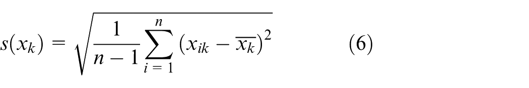
The Type A uncertainty of the pulse waveform is calculated point by point through the Bessel formula as shown in equation (6), which can effectively characterize the local stability of the signal. In equation (6), $n$ represents the number of groups, $k$ represents the number of sampling points, $x$ is the sampling value of the $k^{th}$ sampling point, and $\bar{x_{k}}$ represents the average value of all sampling values at this sampling point. In this paper, 70 groups of waveform data were collected, so $n = 70$ in equation (6) at this time. By calculating the standard uncertainty and relative uncertainty, and comparing them before and after pulse waveform compensation, the accuracy and reliability of the measurement results can be more comprehensively evaluated.

s (x_{k}) = \sqrt{\frac{1}{n - 1} \sum_{i = 1}^{n} {(x_{ik} - \bar{x_{k}})}^{2}}

(6)

The standard uncertainty is used to characterize the dispersibility of measured values and directly reflects the degree of dispersion of measurement results. A smaller standard uncertainty indicates that the measurement results are more concentrated. The standard uncertainties of the 3G–9G group signals before and after compensation are shown as the red lines in Figures 13 and 14. According to the test results, the maximum values of uncertainty appear at the rising and falling edges of the pulse signal. The maximum Type A uncertainty in the original data is 0.035 V, while that in the compensated data is 0.0227 V, representing a decrease of 35.1%. This indicates that the original data has high dispersion and the time-base jitter has a significant impact on the waveform. Meanwhile, the good consistency of repeated measurements shows that the time-base jitter of the oscilloscope has been compensated, demonstrating that the jitter measurement background of the oscilloscope has a good compensation effect.¹⁵

Figure 13.

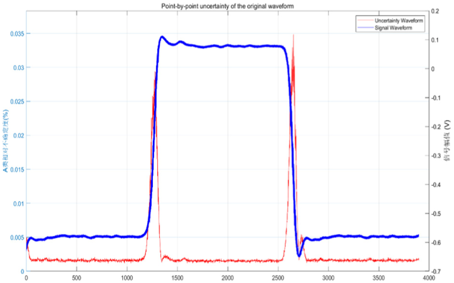
Type A standard uncertainty of original data.

Figure 14.

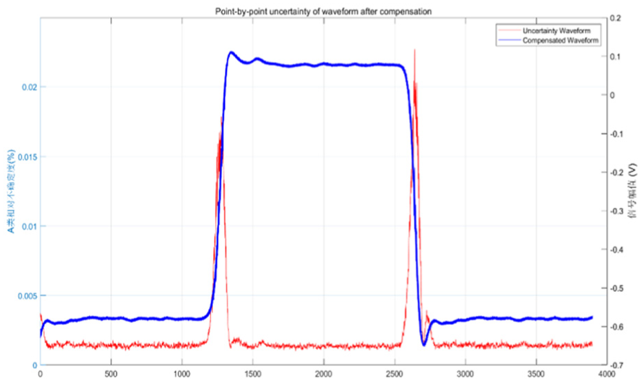
Type A standard uncertainty of compensated data.

The relative uncertainty is the ratio of the standard uncertainty to the measured value, used to measure the proportion of uncertainty in the measurement result. A smaller relative uncertainty indicates higher measurement accuracy. Calculations show that the relative uncertainty of points near the zero point in the amplitude of the rising and falling edges is extremely high. The analysis reveals that this is caused by the signal amplitude (as the denominator) being close to zero. Excluding this part of the data in this paper is consistent with the uncertainty evaluation theory. The specific approach is as follows: taking 0 V as the center, selecting ±10% of the amplitude, and performing the same exclusion operation on both the pre-compensation and post-compensation waveforms. The relative uncertainties of the 3G–9G group signals before and after compensation are shown in Figures 15 and 16. The maximum original point-by-point relative uncertainty is 60.6779%, and it decreases to 39.6165% after compensation, indicating a significant reduction in relative uncertainty and good compensation effect.

Figure 15.

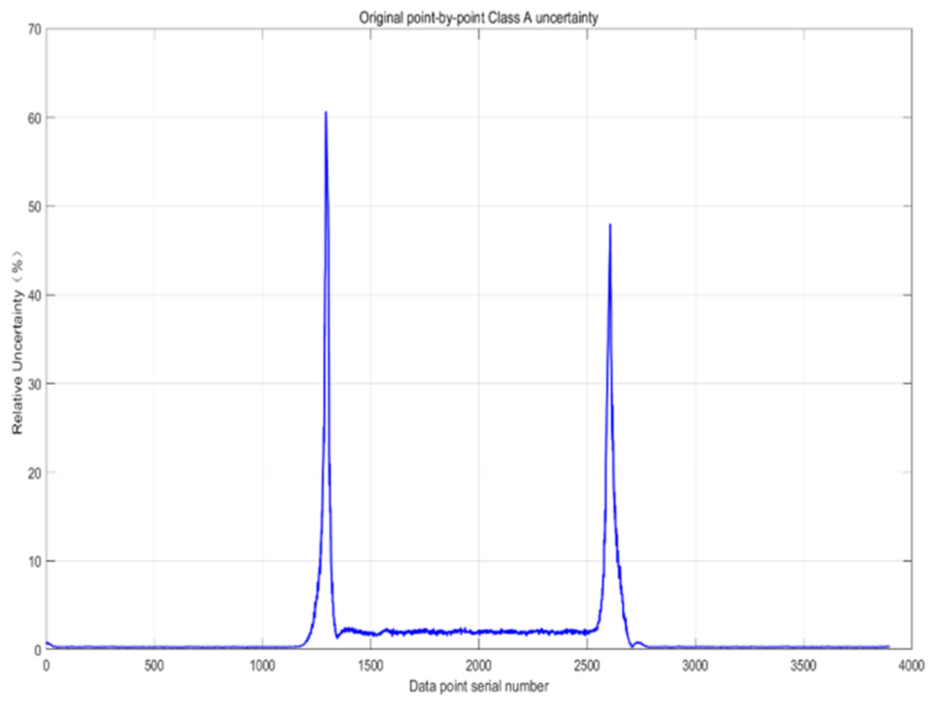
Relative uncertainty of original data.

Figure 16.

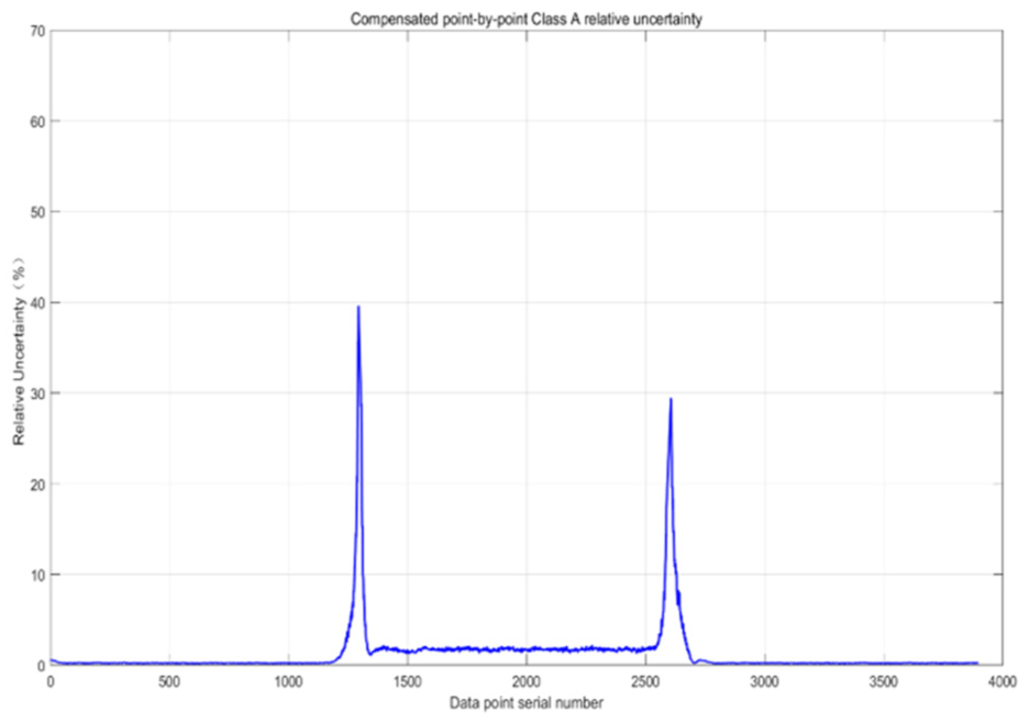
Relative uncertainty of compensated data.

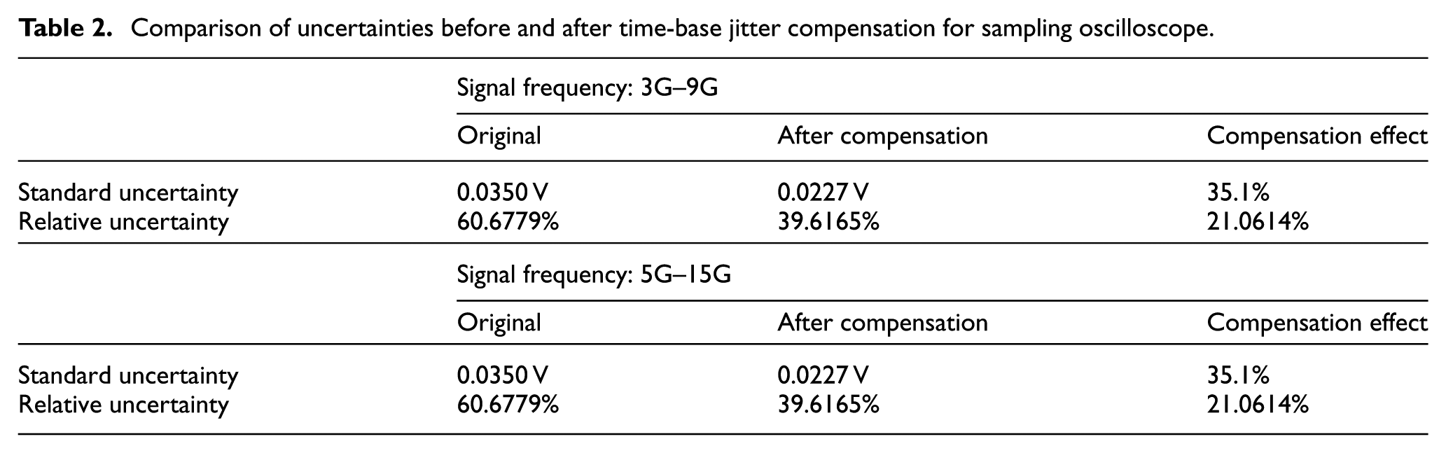
This paper only lists and compares the results of amplitude standard uncertainty and relative uncertainty of pulse signals before and after time-base jitter compensation for the sampling oscilloscope, as shown in Table 2.

Table 2.

Comparison of uncertainties before and after time-base jitter compensation for sampling oscilloscope.

	Signal frequency: 3G–9G
	Original	After compensation	Compensation effect
Standard uncertainty	0.0350 V	0.0227 V	35.1%
Relative uncertainty	60.6779%	39.6165%	21.0614%
	Signal frequency: 5G–15G
	Original	After compensation	Compensation effect
Standard uncertainty	0.0350 V	0.0227 V	35.1%
Relative uncertainty	60.6779%	39.6165%	21.0614%

Conclusions

This study established a three-channel synchronous measurement system where the measured signal is a pulse. Utilizing the Orthogonal Distance Regression algorithm and interpolation algorithm, the method of Type A uncertainty was employed to evaluate the impact of time-base jitter of the broadband sampling oscilloscope on the measurement results. The time-base jitter value of the pulse signal can be compensated by up to 38.3%; analysis shows that the Type A uncertainty has decreased significantly, the Type A uncertainty of the signal can be compensated by up to 35.1%, and the relative uncertainty can be compensated by up to 21.0614%.

The research results indicate that the three-channel synchronous measurement system combined with the orthogonal distance regression algorithm and linear interpolation algorithm can effectively compensate for the time-base jitter of sampling oscilloscopes in precise measurements of pulse signals, providing a solution for accurate measurement of pulse signals.

Footnotes

ORCID iDs

Kaige Man

Weibin Xie

Ethical considerations

This study does not involve ethical issues because the research content does not involve human/animal subjects or sensitive data, and all data in this study were generated through actual measurements.

Informed consent

This study does not involve human subjects, so informed consent is not required.

Author contributions

All authors have contributed to the work presented in this paper and is reflected in this paper.

Funding

The authors disclosed receipt of the following financial support for the research, authorship, and/or publication of this article: The relevant work of this research paper was supported by the following projects: the “Broadband Sampling Oscilloscope” on National Key Research and Development Program of “Fundamental Research Conditions and Development Program of Major Scientific Instruments” (No.2022YFF0707104), and the National Key Research and Development Program “National Quality Infrastructure System” key special project “Research and Application of Key RF Parameter Measurement Standards for Microelectromechanical Systems” (2022YFF0605902).

Declaration of conflicting interests

The authors declared no potential conflicts of interest with respect to the research, authorship, and/or publication of this article.

Trial registration number/date

This study does not involve clinical trials, so no registration is needed.

Data availability statement

Data can be obtained from the corresponding author upon request.

References

Zhu

Sun

Chen

, et al. Measurements and calculation methods of jitter in broadband sampling oscilloscope. In: 2023 IEEE 16th International Conference on Electronic Measurement & Instruments (ICEMI), Harbin, China, 2023, pp.81–85.

Zhu

Cheng

Sun

, et al. Estimation of time base distortion of high speed sampling oscilloscope based on trust-region reflection least square method. In: 2023 IEEE 16th International Conference on Electronic Measurement & Instruments (ICEMI), Harbin, China, 2023, pp.91–97.

Cho

Lee

Kang

, et al. Calibration of sample-time error in a sampling oscilloscope and uncertainty analysis. In: 2016 Conference on Precision Electromagnetic Measurements (CPEM 2016), Ottawa, ON, Canada, 2016, pp. 1–2. doi:10.1109/CPEM.2016.7540669.

Hale

Wang

Williams

, et al. Compensation of random and systematic timing errors in sampling oscilloscopes. IEEE Trans Instrum Meas 2006; 55(6): 2146–2154.

Zhu

Cheng

Zhao

, et al. A new weight setting method for estimating ODR of sampling oscilloscope time base jitter. Measurement 2025; 242: 116024.

IEC. Transitions, pulses and related waveforms – Terms, definitions and algorithms (IEC 60469:2013) [S]. International Electrotechnical Commission; 2013.

IEEE. IEEE 2414-2020 Standard for jitter and phase noise [Standard]. Institute of Electrical and Electronics Engineers; 2020.

IEEE standard for Digitizing Waveform Recorders. IEEE Std 1057-2017 (Revision of IEEE Std 1057-2007) 2018; p.1

N1000A DCA-X and N1002A Optimization Controller Wide Bandwidth Oscilloscope Mainframe, Modules, and N1002A Optimization Controller [EB/OL]. USA. May 14, 2025. https://www.keysight.com.cn/cn/zh/assets/7018-06303/

10.

Hale

Williams

Dienstfrey

Waveform metrology: signal measurements in a modulated world. Metrologia 2018; 55(5): S135–S151.

11.

Bobreshov

Zhabin

Stepkin

, et al. Ultra-short pulse generator with back edge shaper. In: 2019 Radiation and Scattering of Electromagnetic Waves (RSEMW), Divnomorskoe, Russia, 2019, pp.204–207.

12.

Guide ISO. Guide to the expression of uncertainty in measurement — Part 1: Introduction. International Organization for Standardization, 2024.

13.

Joint Committee for Guides in Metrology (JCGM). Guide to the expression of uncertainty in measurement (GUM): supplement 2 - extension to any number of output quantities [EB/OL]. 2011.

14.

Zhu

Sun

Man

, et al. Analysis and improvement of oscilloscope jitter measurement floor based on simulation experiments. In Proceedings of the 2nd International Seminar on Artificial Intelligence, Networking and Information Technology - ANIT; 2024. ISBN 978-989-758-677-4, SciTePress, pp.391–396.

15.

Jitter. 2025. https://helpfiles.keysight.com/scopes/FlexDCA-UG/Content/Topics/Oscilloscope-Mode/Time-Measurements/jitter_scope.htm

Research on time-base jitter compensation of broadband sampling oscilloscope in precise measurement of pulse signals