Assessing the condition of a π-shaped steel–concrete composite girder bridge via two-dimensional spatial load-driven influence surface identification

Abstract

Structural damage continuously accumulates with the extension of bridge service life, posing significant threats to bridge safety and operational functionality. Traditional bridge inspection and assessment methods rely primarily on static load tests or localized sensor monitoring, which struggle to comprehensively reflect dynamic responses under vehicular loads and multiaxial load effects, resulting in notable limitations. In response to the aforementioned challenges, a novel bridge condition assessment methodology utilizing influence surfaces is developed in this investigation. This approach integrates two-dimensional dynamic vehicle loads, incorporates regularization techniques, and employs algorithms such as singular value decomposition (SVD) and variational mode decomposition (VMD) to identify structural influence lines and influence surfaces on bridges. The Sutai Expressway Tongfu No.3 bridge, a steel–concrete composite beam bridge, was used as a case study; a finite element model was established, and a vehicle–bridge coupled dynamic analysis was conducted. By introducing two-dimensional vehicle loads, the identification accuracy and damage detection capability of the proposed method were validated. The results demonstrate that the proposed method effectively eliminates interference from vehicle dynamic effects and multiaxial load coupling, enabling the precise identification of both damage locations and severity levels in bridges, with an identification error of less than 5%.

Introduction

As long-term service transportation infrastructure forms, bridges experience significantly increased probabilities of damage accumulation with extended service under the coupled effects of environmental erosion, long-term load effects, material degradation, and fatigue.^1,2 Therefore, efficient and accurate bridge condition assessment methods are urgently needed. ³ Among the condition assessment methods used for widely distributed small-to-medium conventional bridges, traditional static load tests, although reliable, require traffic closures and concentrated load applications, presenting engineering challenges such as prolonged timelines and high costs. Recent innovations enable load testing without traffic closure. Zhou et al. ⁴ deployed artificial truck fleets in open traffic, achieving spatiotemporal load mapping via computer vision and hybrid simulation, and achieved health assessment of the bridge. The influence line and influence surface information can reflect structural state characteristics, making their utilization critical for evaluating bridge service performance under different operational conditions.

Current research on bridge structural damage identification and condition assessment based on influence lines/surfaces focuses primarily on two aspects: (1) obtaining structural influence line/surface information through experimental testing and (2) identifying damage and assessing structural conditions by comparing identified influence line/surface data with initial state information.

The earliest influence line identification method was the point-by-point graphical approach proposed by O’Brien, ⁵ which was later improved through least squares optimization. ⁶ Zheng et al. ⁷ integrated regularization techniques with least squares QR decomposition to establish a novel influence line identification theory. Concurrently, Chen et al. ⁸ developed a bridge influence line identification method using Tikhonov regularization and B-spline curves, significantly enhancing identification efficiency and accuracy. For influence surface identification, Yu et al. ⁹ simplified vehicle loads as point loads and employed linear interpolation to derive influence surfaces from influence lines. To extend this work, Zheng et al. ¹⁰ incorporated the spatial effects of two-dimensional vehicle loads for influence surface identification. Because influence lines contain structural stiffness information, studies have shown that bridge condition assessment and damage analysis can be conducted using influence line differences before and after damage.^11–14 Wang et al. ¹⁵ proposed damage localization via quadratic differences in influence lines, whereas He et al. ¹⁶ defined damage localization indices on the basis of variation curves and enclosed areas of bridge elements before/after damage, achieving quantitative damage localization.

Most existing influence line/surface identification methods simplify vehicle loads as linear loads, whereas real-world vehicle load distributions inevitably exhibit partial loading characteristics. Thus, considering two-dimensional actual vehicle loads enables a more realistic derivation of structural influence lines/surfaces. Furthermore, vehicle load analyses typically simplify vehicles as moving loads, with limited consideration of vehicle–bridge coupled vibration effects. This paper proposes a novel methodology for structural influence line/surface identification and damage detection under advanced vehicle–bridge interaction strategies.

Framework of bridge condition assessment via the influence surface

Influence line identification methods

Construction of an influence line identification mathematical model

The quasistatic response of a bridge under moving vehicles can be considered the superposition of bridge responses induced by individual axles, which can be simplified as the successive application of moving forces along an influence line. On the basis of the physical interpretation of influence lines, the quasistatic response R of a bridge under moving vehicles can be expressed as:

$$R\left(x\right)=G_i\phi (x)$$

(1)

where G _i is the vehicle weight and φ(x) is the influence line function of the bridge.

Vehicle load simulation methods include point load representation (PLR), line load representation (LLR), and two-dimensional spatial load representation (SLR). ¹⁰ Both the PLR and LLR methods simplify the simulation of vehicle–bridge coupled vibrations but neglect transverse load effects during simplification. When the vehicle’s center of gravity deviates from its transverse central axis, the influence lines obtained through the PLR and LLR simulations exhibit lateral deviations. Therefore, vehicle load corrections are implemented here via the SLR theory.

A two-dimensional vehicle load can be regarded as the superposition of two line loads. According to influence line theory, the bridge response R can be expressed as:

$$\mathbf{R}={\mathbf{W}}_L^T{\mathbf{\Phi }}^L+{\mathbf{W}}_R^T{\mathbf{\Phi }}^R$$

(2)

For the convenience of calculation, equation (2) is written in matrix form:

$$\mathbf{R}=\mathbf{W}\mathbf{\Phi }=\left[\begin{array}{cc}{\mathbf{W}}_L^T\hfill & {\mathbf{W}}_R^T\hfill \end{array}\right]\left[\begin{array}{c}{\mathbf{\Phi }}^L\hfill \\ \multicolumn{1}{c}{{\mathbf{\Phi }}^R}\end{array}\right]$$

(3)

where ${\mathbf{W}}_L^T$ and ${\mathbf{W}}_R^T$ are the left and right wheel load matrices of the vehicle, respectively, and where ${\mathbf{\Phi }}^L$ and ${\mathbf{\Phi }}^R$ are the influence lines at the tracks of the left and right wheels, respectively. ${\mathbf{\Phi }}^L={\left[\begin{array}{ccccc}{I}_1^L\hfill & I_2^L\hfill & I_3^L\hfill & \cdots \hfill & I_{K-C_N}^L\hfill \end{array}\right]}^T$ ; ${\mathbf{\Phi }}^R={\left[\begin{array}{ccccc}{I}_1^R\hfill & I_2^R\hfill & I_3^R\hfill & \cdots \hfill & I_{K-C_N}^R\hfill \end{array}\right]}^T$ , where k is the number of discrete data points in the data acquisition signal time history of the bridge, and C _N is the sampling point difference between the last two axes.

$$W_L={\left[\begin{array}{ccccccccccccccc}{P}_1^L\hfill & 0\hfill & \cdots \hfill & P_2^L\hfill & 0\hfill & \cdots \hfill & P_3^L\hfill & 0\hfill & \cdots \hfill & P_N^L\hfill & 0\hfill & \cdots \hfill & \cdots \hfill & \cdots \hfill & 0\hfill \\ \multicolumn{1}{c}{0}& P_1^L\hfill & 0\hfill & \cdots \hfill & P_2^L\hfill & 0\hfill & \cdots \hfill & P_3^L\hfill & 0\hfill & \cdots \hfill & P_N^L\hfill & 0\hfill & \cdots \hfill & \cdots \hfill & 0\hfill \\ \multicolumn{1}{c}{0}& 0\hfill & P_1^L\hfill & 0\hfill & \cdots \hfill & P_2^L\hfill & 0\hfill & \cdots \hfill & P_3^L\hfill & 0\hfill & \cdots \hfill & P_N^L\hfill & 0\hfill & \cdots \hfill & 0\hfill \\ \multicolumn{1}{c}{⋮}& \ddots \hfill & \ddots \hfill & \ddots \hfill & \ddots \hfill & \ddots \hfill & \ddots \hfill & \ddots \hfill & \ddots \hfill & \ddots \hfill & \ddots \hfill & \ddots \hfill & \ddots \hfill & \ddots \hfill & ⋮\hfill \\ \multicolumn{1}{c}{⋮}& \ddots \hfill & \ddots \hfill & \ddots \hfill & \ddots \hfill & \ddots \hfill & \ddots \hfill & \ddots \hfill & \ddots \hfill & \ddots \hfill & \ddots \hfill & \ddots \hfill & \ddots \hfill & \ddots \hfill & ⋮\hfill \\ \multicolumn{1}{c}{0}& 0\hfill & \cdots \hfill & 0\hfill & 0\hfill & P_1^L\hfill & 0\hfill & \cdots \hfill & P_2^L\hfill & 0\hfill & \cdots \hfill & P_{N-1}^L\hfill & 0\hfill & \cdots \hfill & P_N^L\hfill \end{array}\right]}_{(K-C_N)\times K}$$

(4)

$$W_R={\left[\begin{array}{ccccccccccccccc}{P}_1^R\hfill & 0\hfill & \cdots \hfill & P_2^R\hfill & 0\hfill & \cdots \hfill & P_3^R\hfill & 0\hfill & \cdots \hfill & P_N^R\hfill & 0\hfill & \cdots \hfill & \cdots \hfill & \cdots \hfill & 0\hfill \\ \multicolumn{1}{c}{0}& P_1^R\hfill & 0\hfill & \cdots \hfill & P_2^R\hfill & 0\hfill & \cdots \hfill & P_3^R\hfill & 0\hfill & \cdots \hfill & P_N^R\hfill & 0\hfill & \cdots \hfill & \cdots \hfill & 0\hfill \\ \multicolumn{1}{c}{0}& 0\hfill & P_1^R\hfill & 0\hfill & \cdots \hfill & P_2^R\hfill & 0\hfill & \cdots \hfill & P_3^R\hfill & 0\hfill & \cdots \hfill & P_N^R\hfill & 0\hfill & \cdots \hfill & 0\hfill \\ \multicolumn{1}{c}{⋮}& \ddots \hfill & \ddots \hfill & \ddots \hfill & \ddots \hfill & \ddots \hfill & \ddots \hfill & \ddots \hfill & \ddots \hfill & \ddots \hfill & \ddots \hfill & \ddots \hfill & \ddots \hfill & \ddots \hfill & ⋮\hfill \\ \multicolumn{1}{c}{⋮}& \ddots \hfill & \ddots \hfill & \ddots \hfill & \ddots \hfill & \ddots \hfill & \ddots \hfill & \ddots \hfill & \ddots \hfill & \ddots \hfill & \ddots \hfill & \ddots \hfill & \ddots \hfill & \ddots \hfill & ⋮\hfill \\ \multicolumn{1}{c}{0}& 0\hfill & \cdots \hfill & 0\hfill & 0\hfill & P_1^R\hfill & 0\hfill & \cdots \hfill & P_2^R\hfill & 0\hfill & \cdots \hfill & P_{N-1}^R\hfill & 0\hfill & \cdots \hfill & P_N^R\hfill \end{array}\right]}_{(K-C_N)\times K}$$

(5)

$$C_N=\frac{\mathrm{df}}{v}$$

(6)

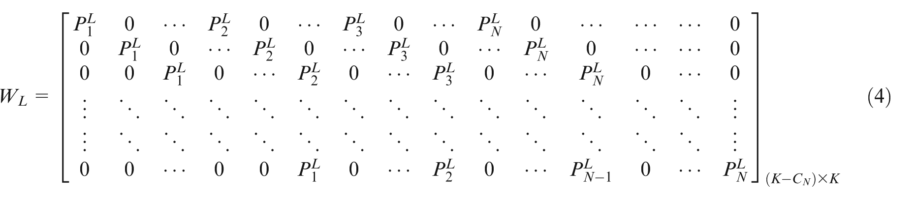
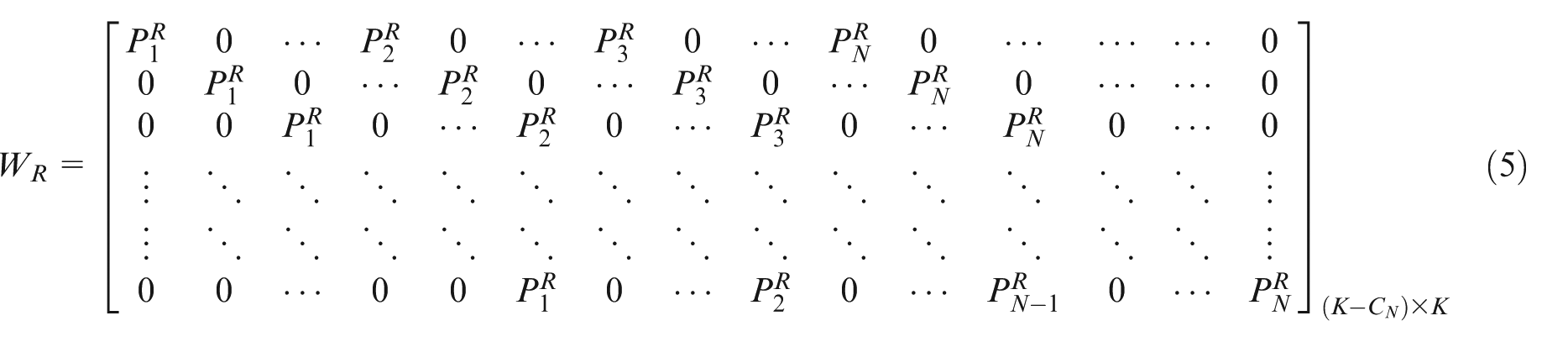
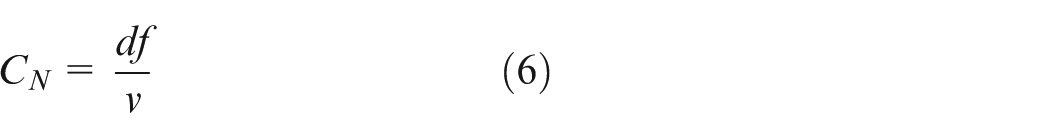
where d represents the distance between the last two axles of the vehicle, f denotes the sampling frequency of the data acquisition equipment, and v indicates the vehicle velocity.

To efficiently utilize and conveniently solve the influence lines, the running strategy of the test vehicle during measurement requires adjustment. An inspection vehicle performs shuttle running on the bridge deck, with each crossing laterally shifted by one vehicle width. This ensures that the wheel track on one side during each crossing coincides with that of the previous crossing, as illustrated in Figure 1.

Figure 1.

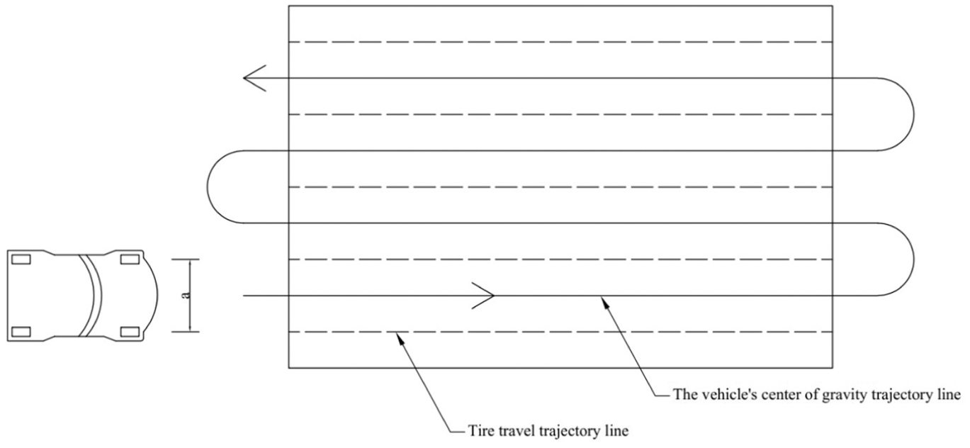
New driving strategy.

The measured bridge time–history responses require preprocessing through variational mode decomposition (VMD). The dominant frequencies of the intrinsic mode function (IMF) components are obtained via fast Fourier transform (FFT), and the IMF components with frequencies exceeding the bridge fundamental frequency are eliminated as dynamic components, thereby deriving the purified bridge time–history responses. ¹⁷

Regularization and singular value decomposition

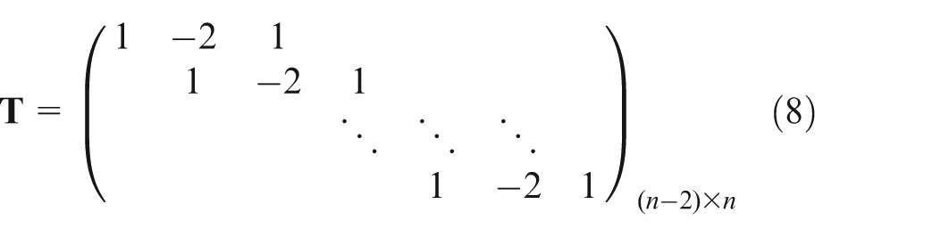
The direct solution of equation (3) requires the inversion of L, which necessitates W to be a square matrix. Therefore, regularization is applied to W. The optimized objective function is introduced as follows:

$$min[\Vert \mathbf{R}-\mathbf{W}\mathbf{\Phi }{\Vert }_2^2+\lambda \Vert \mathbf{T}\mathbf{\Phi }{\Vert }_2^2]$$

(7)

where T is the second-order difference matrix ¹⁸ and where λ is the regularization parameter for adjusting the weight of the penalty function.^19,20

$$\mathbf{T}={\left(\begin{array}{ccccccc}1\hfill & -2\hfill & 1\hfill & \hfill & \hfill & \hfill & \hfill \\ \hfill & 1\hfill & -2\hfill & 1\hfill & \hfill & \hfill & \hfill \\ \hfill & \hfill & \hfill & \ddots \hfill & \ddots \hfill & \ddots \hfill & \hfill \\ \hfill & \hfill & \hfill & \hfill & 1\hfill & -2\hfill & 1\hfill \end{array}\right)}_{(n-2)\times n}$$

(8)

Owing to the large volume of measured data, the calculation efficiency is relatively low. To improve the calculation efficiency, singular value decomposition (SVD) is introduced, and the matrix W is expressed as:

The matrix is reconstructed as:

$$\mathbf{W}=U\Sigma V^T=\sum _i^k{u}_i{e}_i{v}_i^T$$

(9)

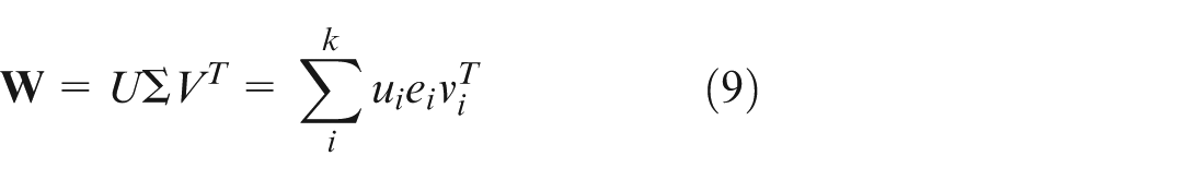
where U is the matrix of m×n, where u _i is the left singular vector; Σ is a matrix of m×n, where e _i is a singular value; and V is a matrix of m×n, where v _i is a right singular vector.

The matrix is reconstructed as:

$$\mathbf{\Phi }=\sum _i^n\frac{u_i^T{\mathbf{R}}_t}{e_i}{v}_i$$

(10)

Owing to the presence of measurement noise in addition to the response caused by moving vehicles in the measured structure, the measured bridge response can be expressed as:

$${\mathbf{R}}_t={\mathbf{R}}_c+r$$

(11)

where R _c is the response caused by the vehicle and r is the measurement noise.

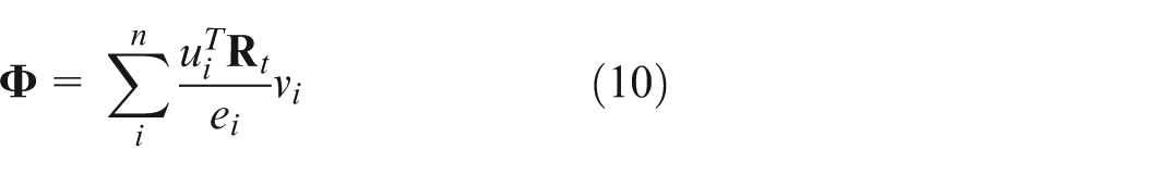
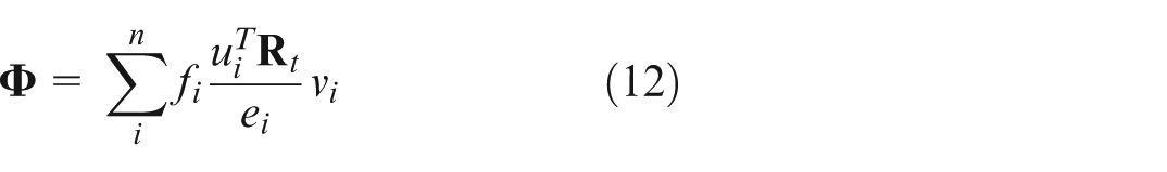
When the matrix in equation (10) has high dimensionality (i.e. singular values e _i are small), the presence of measurement noise and errors in R _t may lead to significant error components in the solution. To address this, a filtering factor is introduced into the equation for correction:

$$\mathbf{\Phi }=\sum _i^n{f}_i\frac{u_i^T{\mathbf{R}}_t}{e_i}{v}_i$$

(12)

On the basis of equation (4), by differentiating the unknown solution $\Phi$ with respect to the Euclidean norm, the regularization can be formulated as:

$$({\mathbf{W}}^{\mathrm{T}}\mathbf{W}+{\lambda }^2{\mathbf{T}}^{\mathrm{T}}\mathbf{T})\Phi ={\mathbf{W}}^{\mathrm{T}}\mathbf{R}$$

(13)

By employing the coefficients from equation (13) as the filtering factor in equation (12) and reformulating them through SVD, the solution can be expressed as:

$$\Phi =\sum _i^n\frac{e_i^2}{e_i^2+{\lambda }^2{t}_i^2}\frac{u_i^T{\mathbf{R}}_t}{e_i}{v}_i$$

(14)

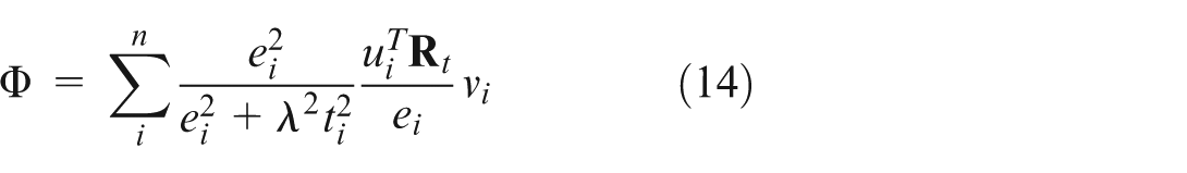
where t _i is the element in T^TT.

Comparing equation (12) and formula equation (14), it can be concluded that $f_i=\frac{e_i^2}{e_i^2+{\lambda }^2{t}_i^2}$ . The core function of fi is to modulate the weight of the SVD component.

• For large ei (dominant signal components), fi ≈ 1, preserving critical structural information.

• For small ei (noise-sensitive components), fi ≈ 0, suppressing amplification of measurement noise.

This mechanism transforms the reconstruction process from directly solving pathological equations to weighted separation of signals and noise. $f_i=\frac{e_i^2}{e_i^2+{\lambda }^2{t}_i^2}$

Influence surface identification method

The bridge influence surface can be regarded as the lateral extension of influence lines within the vertical bending deformation reference plane of the beam. Consequently, the influence surface can be reconstructed through lateral interpolation of influence lines identified at different transverse positions. The implementation procedure includes installing necessary sensors on the bridge, dividing the deck into grids, applying vehicular loads along individual lanes, recording structural responses, identifying lane-specific influence lines via regularization and SVD, and finally reconstructing the influence surface via lateral interpolation of all the lane-derived influence lines.

Damage diagnosis method for steel–concrete composite beam bridges based on influence surfaces

Although the influence surface is usually less sensitive to local damage due to its global nature, some scholars have proposed qualitative and quantitative analysis of bridge damage based on the deflection influence line before and after damage and have demonstrated this method’s effectiveness through numerous numerical and example case studies. ¹¹ The methods mentioned in this article are used to reconstruct high-resolution influence surfaces via lateral interpolation of wheel-path-specific influence lines. To some extent, this can amplify the damage characteristics.

By adopting bridge health monitoring principles, an influence surface matrix is established for a bridge in its initial undamaged state. Localized damage alters the stiffness continuity of the bridge, ultimately modifying its influence surface. Damage identification is achieved by analyzing the difference matrix between the influence surfaces in the damaged and initial states. This relationship is expressed as follows:

$$\begin{array}{c}{\left[\begin{array}{cccc}\mathrm{\Delta }{\Phi }_1\hfill & \mathrm{\Delta }{\Phi }_2\hfill & \cdots \hfill & \mathrm{\Delta }{\Phi }_n\hfill \end{array}\right]}^T\hfill \\ ={\left[\begin{array}{cccc}{\Phi }_1\hfill & {\Phi }_2\hfill & \cdots \hfill & {\Phi }_n\hfill \end{array}\right]}^T-{\left[\begin{array}{cccc}{\Phi }_1^{\prime }\hfill & {\Phi }_2^{\prime }\hfill & \cdots \hfill & {\Phi }_n^{\prime }\hfill \end{array}\right]}^T\hfill \end{array}$$

(15)

where $\left[\begin{array}{cccc}{\Phi }_1\hfill & {\Phi }_2\hfill & \cdots \hfill & {\Phi }_n\hfill \end{array}\right]$ denotes the influence surface matrix of the initial state, $\left[\begin{array}{cccc}{\Phi }_1^{\prime }\hfill & {\Phi }_2^{\prime }\hfill & \cdots \hfill & {\Phi }_n^{\prime }\hfill \end{array}\right]$ represents the influence surface matrix after damage, ${\Phi }_n$ corresponds to the measured n-th initial-state influence line of the bridge, ${{\Phi }^{\prime }}_n$ indicates the measured n-th post-damage influence line, and ${\Phi }_n^{\prime }$ signifies the difference between the n-th influence lines before and after damage.

Case study

The Sutai Expressway Tongfu No.3 Viaduct was used as the engineering case in this study. A numerical simulation model of the bridge in its healthy state was established via ANSYS to derive the initial influence surface matrix. Localized damage was simulated through stiffness reduction, and the proposed methodology was applied to identify the post-damage influence surface matrix, thereby enabling damage detection.

Project overview

Experimental investigations were conducted on the Sutai Expressway Tongfu No.3 Viaduct, which is a five-span continuous steel–concrete composite beam bridge with π-shaped steel girders. The bridge comprises two separate decks (left and right), with each span measuring 30 m. The substructure consists of H-shaped piers supported by bored piles. The deck width is 2 × 16.5 m. The superstructure employs concrete slabs combined with I-shaped composite steel girders. The deck slab is comprised of C50 concrete, whereas ultrahigh performance concrete (UHPC) is implemented at intermediate support locations. Structural steel components are fabricated from Q355D steel. The cross-sectional configuration of a single deck is illustrated in Figure 2.

Figure 2.

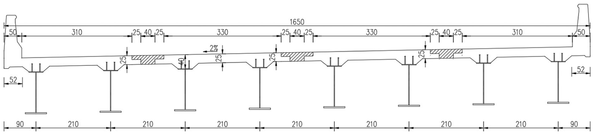
Schematic diagram of a bridge cross-section.

Finite element model establishment

Following design specifications, a two-axle vehicle loading model ²¹ was developed in ANSYS, which is shown in Figure 3(a). The full bridge model contains 2426 elements with a fundamental frequency of 1.4622 Hz. The loading process was discretized into 751 steps at 0.2 m intervals. Each deck was configured with seven virtual lanes (1.8 m width per lane). A two-axle vehicle was modeled as a linear line load, and vehicle–bridge coupled vibration simulations were performed, with the simulation results visualized in Figure 3(b).

Figure 3.

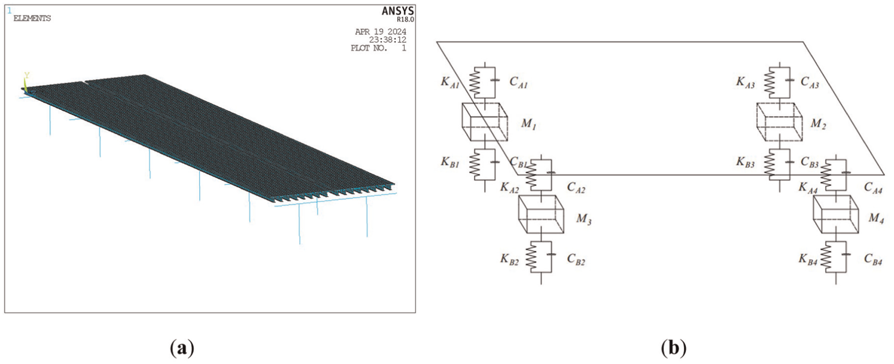
(a) ANSYS finite element model and (b) schematic diagram of the vehicle model.

As shown in Figure 3(b), where M₁, M₂, M₃, and M₄ represent the mass per wheel; K _{A 1}, K _{A 2}, K _{A 3}, and K _{A 4} denote the primary suspension stiffness per wheel; K _{B 1}, K _{B 2}, K _{B 3}, and K _{B 4} indicate the secondary suspension stiffness per wheel; C _{A 1}, C _{A 2}, C _{A 3}, and C _{A 4} correspond to the primary suspension damping coefficients per wheel; and C _{B 1}, C _{B 2}, C _{B 3}, and C _{B 4} represent the secondary suspension damping coefficients per wheel.

Influence surface identification

The mid-span section of the central span in the five-span steel–concrete composite beam was selected as the displacement measurement point. A two-axle vehicle initiated loading from a transverse position of 1.95 m on the bridge deck, with each subsequent crossing laterally shifted by 1.8 m. Seven crossings generated eight wheel tracks for vehicle–bridge coupled vibration analysis. The bridge response under vehicle passage at 0.01 km/h was regarded as the static response, whereas the 60 km/h condition provided dynamic response data. Displacement time–history data extracted from the coupled vibration analysis were used to plot the raw displacement responses for all the wheel tracks (Figure 4(a)). The original displacement response surface was reconstructed through interpolation of these response lines, as shown in Figure 4(b).

Figure 4.

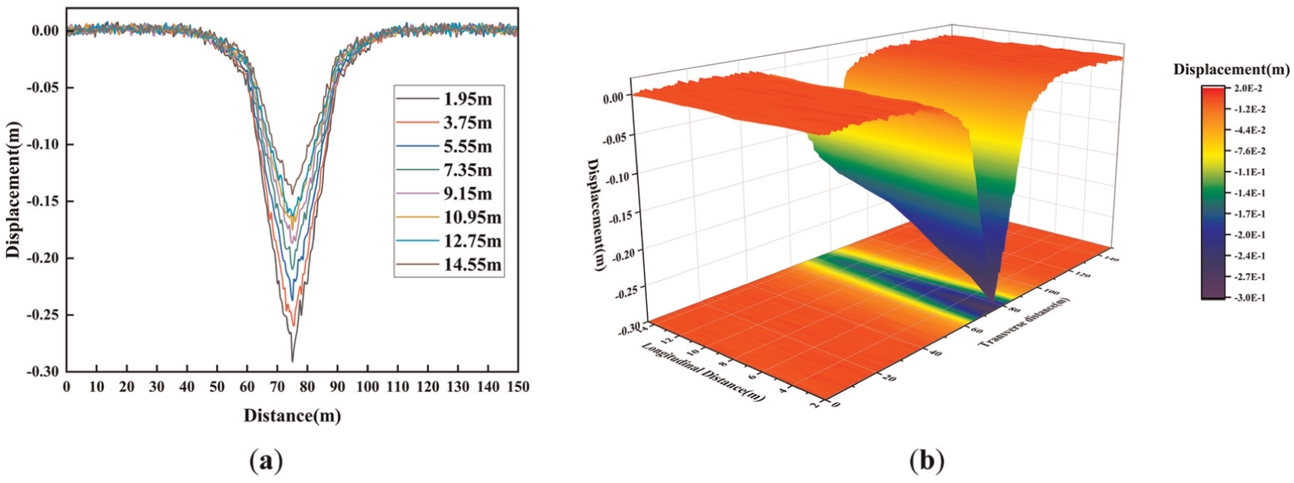
(a) Unfiltered displacement response lines of individual wheel paths and (b) unfiltered displacement response faces of individual wheel paths.

As shown in Figure 4(a), dynamic disturbance phenomena occur when the vehicle crosses the bridge at 60 km/h. Owing to multiaxial effects, the analysis requires 781 loading steps. The dynamic components in the displacement responses were extracted via the VMD method. The specific decomposition results of VMD are shown in Figure 5. The static and quasistatic bridge lane displacement response plots are shown in Figure 6(a) and (b), respectively. The quasistatic and static displacement response surfaces reconstructed via interpolation are presented in Figure 6(c) and (d).

Figure 5.

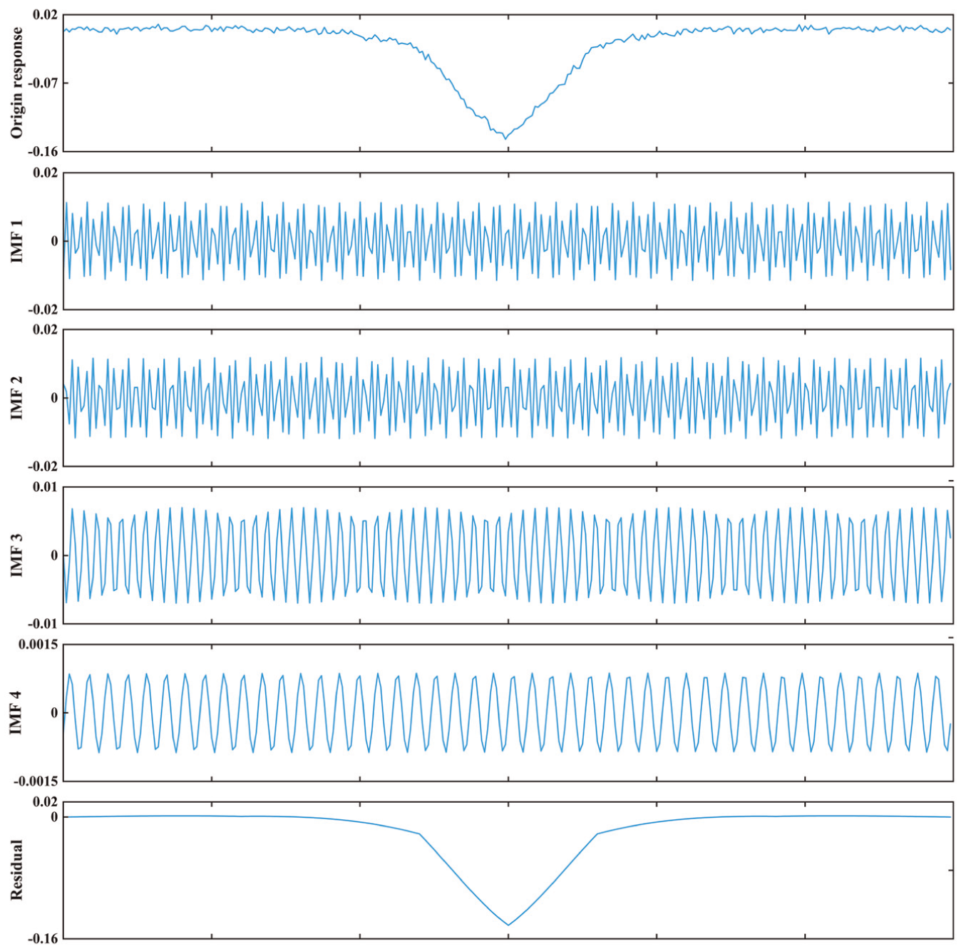
VMD decomposition process.

Figure 6.

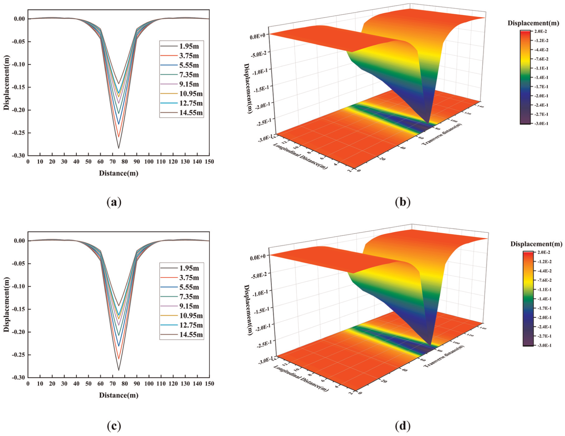
(a) Static bridge lane displacement response line, (b) static displacement response surface, (c) quasistatic bridge lane displacement response line, and (d) quasistatic displacement response surface.

As illustrated in Figure 6, the quasistatic and static displacement response surfaces of the bridge obtained through this method exhibit high consistency, demonstrating the effectiveness of VMD in extracting dynamic components from the responses. However, the processed bridge displacement responses still contain multiaxial coupling effects. To eliminate the influence of vehicle multiaxial effects, L2 regularization was applied to identify the bridge displacement influence lines (Figure 7(a) and (b)). Finally, the bridge displacement influence surfaces were reconstructed via interpolation. The quasistatic and static displacement influence surfaces are presented in Figure 7(c) and (d), respectively.

Figure 7.

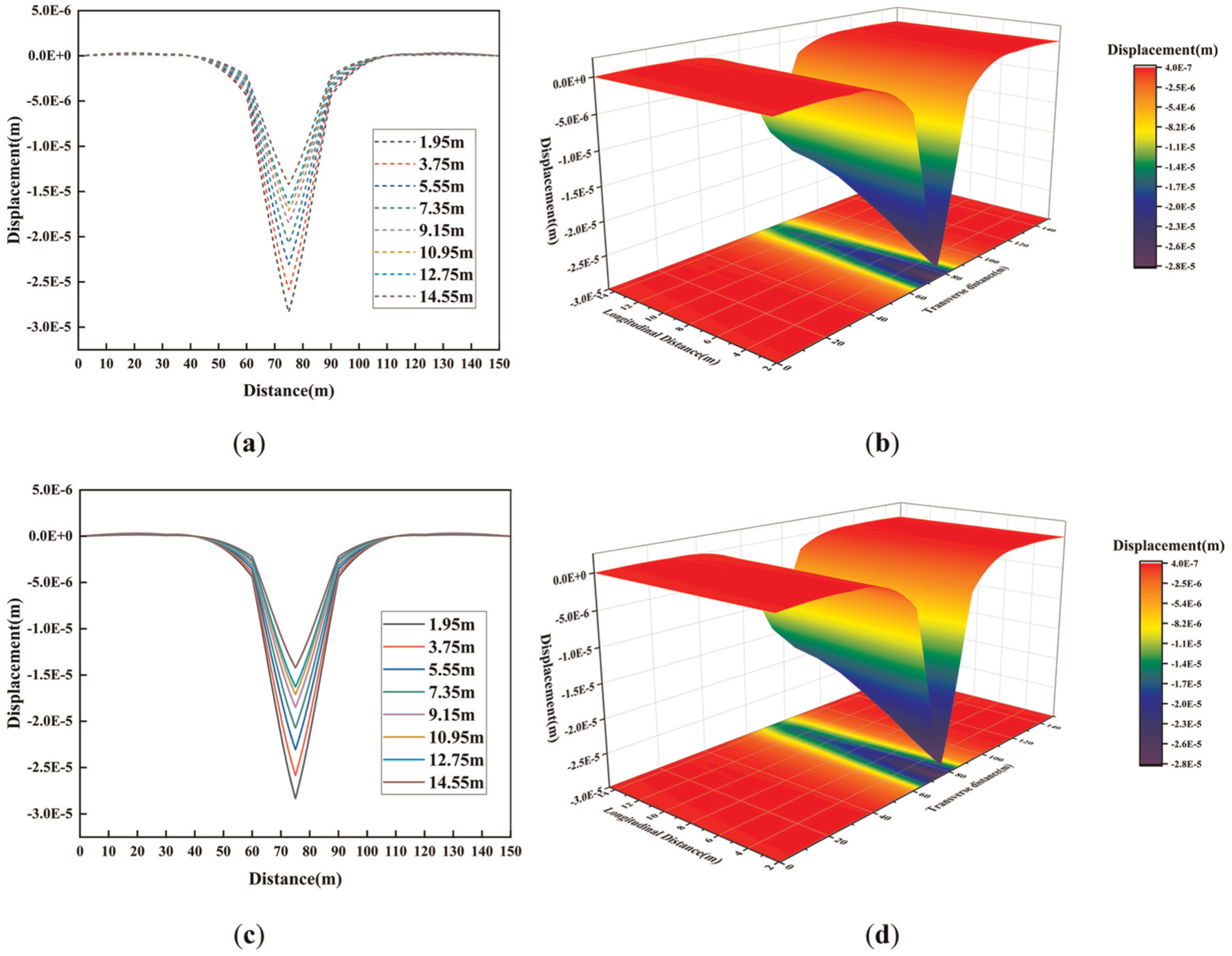
(a) Influence line of static bridge lane displacement, (b) influence surface of static bridge lane displacement, (c) quasistatic bridge lane displacement influence line, and (d) influence surface of quasistatic bridge lane displacement.

As shown in Figure 7, the quasistatic and static displacement influence surfaces of the bridge demonstrate high consistency. Notably, the loading steps are maintained at 751 in this analysis, effectively eliminating the additional steps induced by multiaxial effects.

Error analysis

Error analysis was conducted by comparing quasistatic and static displacement influence surfaces to validate the accuracy of the proposed methodology. The error metrics are defined as follows:

$$e_i=\frac{\sum |S_s-S_{\mathrm{qs}}|}{\sum \left|S_{\mathrm{qs}}\right|}$$

(16)

$$e_{\mathrm{rp}}=\frac{{\left|S_s\right|}_{max}-{\left|S_{\mathrm{qs}}\right|}_{max}}{{\left|S_{\mathrm{qs}}\right|}_{max}}$$

(17)

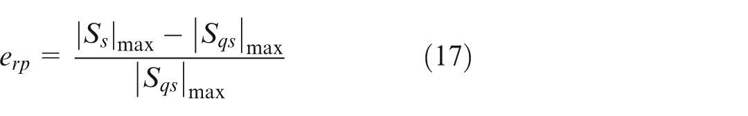
where $e_i$ is the overall relative error; $S_s$ is the static displacement influence surface; $S_{\mathrm{qs}}$ is the quasistatic displacement influence surface; and $e_{\mathrm{rp}}$ is the peak value of the relative error.

The calculated values of $e_i$ and $e_{\mathrm{rp}}$ are 3.147% and 4.663%, respectively. Both are small, indicating that the influence mask obtained via VMD and L2 regularization has a certain accuracy.

Nonoverlapping trajectories will have an impact on the detection results. We perform an overall lateral deviation of the driving trajectory and conduct a vehicle bridge coupling analysis again to compare the analysis errors of the two. The simulation shows that when the lateral deviation is 10 cm, the recognition error of the influence line is less than 5%.

Bridge damage identification

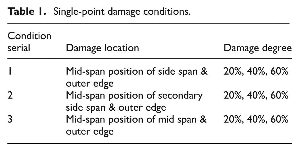
Using the difference in the displacement influence surface before and after damage as a damage index, the feasibility of this method for identifying bridge damage is explored. The stiffness reduction of the damaged bridge element is used to simulate bridge damage. The middle span is selected as the displacement measurement point, and the points simulating bridge damage are shown in Table 1.

Table 1.

Single-point damage conditions.

Condition serial	Damage location	Damage degree
1	Mid-span position of side span & outer edge	20%, 40%, 60%
2	Mid-span position of secondary side span & outer edge	20%, 40%, 60%
3	Mid-span position of mid span & outer edge	20%, 40%, 60%

The influence surface differences under these three loading cases are shown in Figures 8 to 11.

Figure 8.

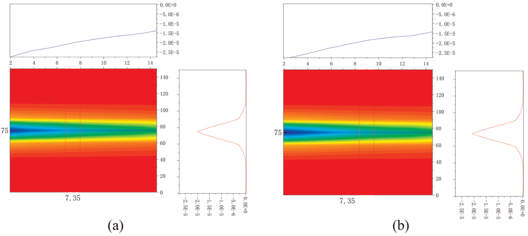
(a) Ideal identification of influence surface and (b) the influence surface of the overall trajectory offset by 10 cm.

Figure 9.

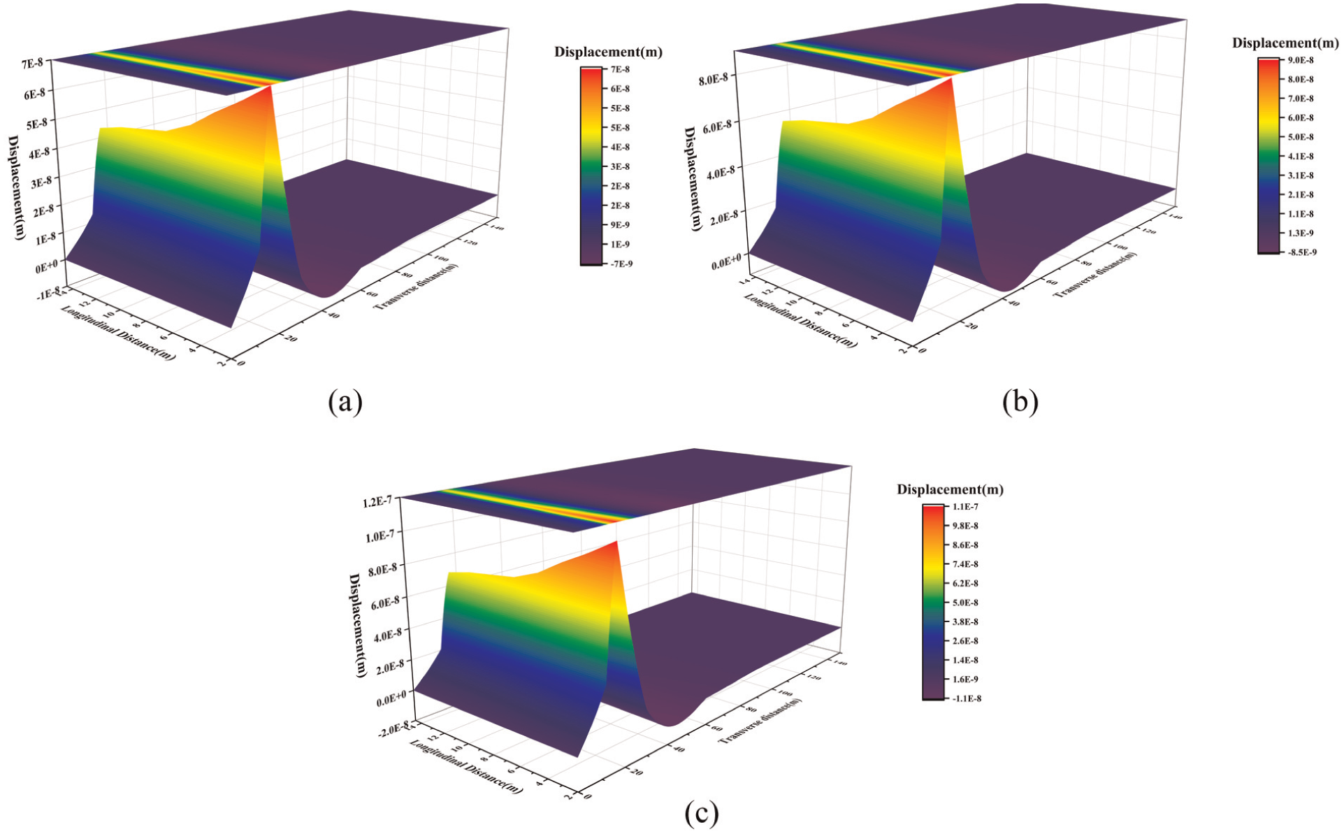
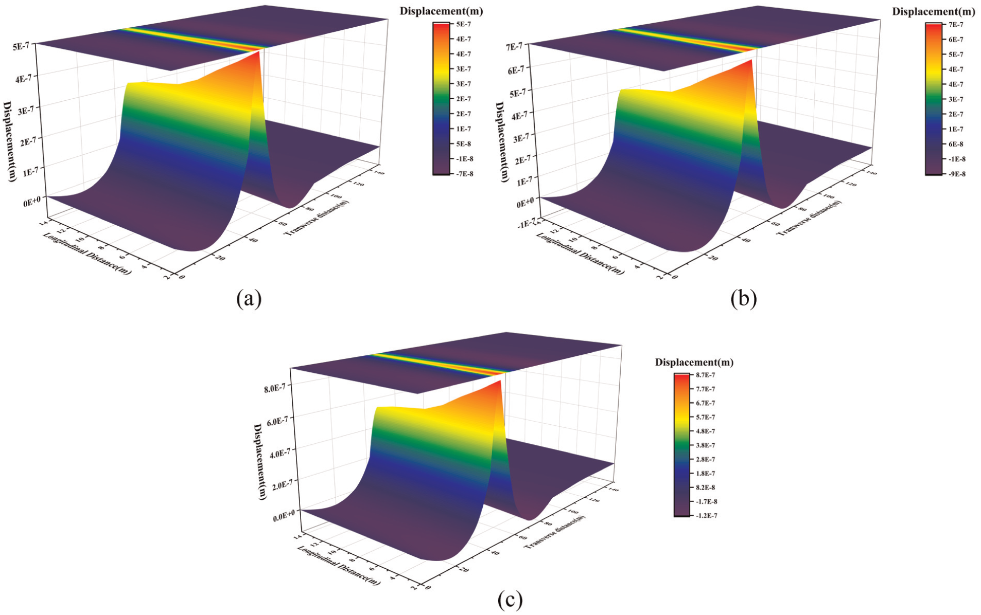
(a) Influence surface under condition 1 and damage 20%, (b) influence surface under condition 1 and damage 40%, and (c) influence surface under condition 1 and damage 60%.

Figure 10.

(a) Influence surface under condition 2 and damage 20%, (b) influence surface under condition 2 and damage 40%, and (c) influence surface under condition 2 and damage 40%.

Figure 11.

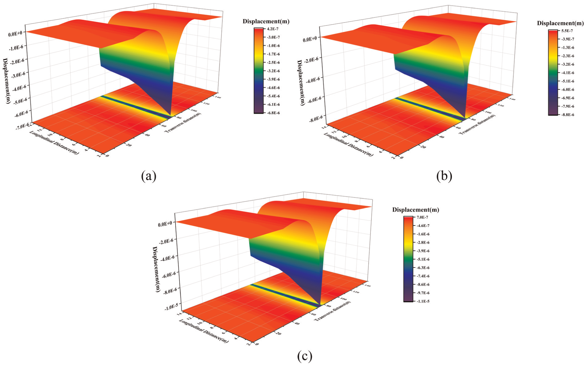
(a) Influence surface under condition 3 and 20% damage, (b) influence surface under condition 3 and 40% damage, and (c) influence surface under condition 3 and 40% damage.

The displacement influence surface differences at single-point damage locations exhibit abrupt changes, with displacement differences increasing proportionally to damage severity. The influence surface difference patterns remain consistent across varying damage levels at the same damage-prone location. In the transverse direction, the displacement differences decay with increasing distance from the damage location. These characteristics enable precise damage localization. By establishing a correlation model between damage severity and displacement differences through multilevel damage simulations, a quantitative damage severity assessment can be achieved.

Conclusions

Through the above analysis, three main conclusions are drawn:

The proposed method effectively eliminates dynamic components and multiaxial vehicle effects from bridge responses. The overall relative error and peak relative error between the quasistatic and static influence surfaces remain below 5%, demonstrating high accuracy.

Damage localization is achieved by identifying abrupt changes in the influence surface differences. A quantitative damage severity assessment is enabled through multilevel damage simulations that establish damage severity indices.

An analysis of influence line differences across damage levels reveals consistent geometric patterns at identical damage-prone locations. Displacement differences exhibit monotonic growth with increasing damage severity.

The method proposed in this article is based on theoretical analysis and numerical simulation. In practice, the inability of vehicle trajectories to completely coincide is a problem. Therefore, we hope to focus on the impact of trajectory line noncoincidence on the analysis results through subsequent practical experimental work. Field studies should be conducted in the future to further investigate the performance of the proposed method for real applications.