
Abstract
In this study, long short-term memory (LSTM) was used for real-time forecasting of the demolding force in an injection molding process. The melt temperature, mold temperature, filling time, and packing pressure were evaluated in three cases by using a quasi-experimental method. Three optimization algorithms, namely, stochastic gradient descent with momentum (SGDM), root mean squared propagation (RMSPROP), and adaptive moment estimation (ADAM), were used to train, test, and evaluate LSTM models based on time-series demolding force data. Model performance was evaluated using the root mean square error (RMSE) and coefficient of determination (R2). The results showed that all the optimization algorithms yielded satisfactory predictions, with the ADAM-LSTM delivering the best performance. Specifically, the ADAM-LSTM achieved a minimum RMSE of 3.55 N and a maximum R2 of 99.45% under one specific condition, indicating excellent agreement between the predicted and actual demolding force profiles. These results confirm that the LSTM architecture, particularly when optimized with ADAM, effectively captures the nonlinear and temporal dynamics of demolding force in injection molding. In addition, the impact assessment of the time-step prediction validated the model’s ability to predict force progression over successive molding cycles. Overall, the proposed LSTM-based model provides a reliable tool for forecasting and monitoring the demolding phase in injection molding, enabling real-time process control and experimental validation.
Introduction
The application of forecasting techniques is a crucial approach for time-series data-driven analysis, especially in prediction. Given the significance of this technique in relation to the demolding force of an injection molding cycle, forecasting the demolding force in real-time scenarios becomes an essential consideration. The demolding force refers to the force required for releasing a molded part from the mold.1–6 The demolding force is evaluated to determine the optimal conditions for achieving improved quality of the molded parts.7–10 Moreover, it is imperative to actively monitor and effectively control the demolding force in real-time throughout the injection molding process. The real-time monitoring of time-varying variables, including the demolding force, plays an important role in the injection molding process because it can provide feedback about quality to the process control system.11–13 The results collected by the process control system over a cycle form time-series data.
A time-series forecasting system predicts a system’s behavior in the future based on information about the current and past status of the system. 14 Zhao et al. highlighted the importance of time-varying evaluations and proposed a strategy for quality analysis and prediction of a typical slow time-varying batch process and start-up process for injection molding. 15 The importance of time-varying evaluations of cavity pressures was verified through an analytical approach to determine the in-plane shrinkage from a simple, closed-form expression for the residual stress. 16 Similarly, a time-variant model in a model-based predictive controller was employed to track a given cavity pressure reference. 17 This approach not only enabled the tailoring of the convergence behavior of the parameter estimation for safe operation and good performance but also allowed rapid control of the topology for new processing conditions. In addition, the time-varying evaluation enables end-users of the injection molding process to optimize the process operations and part geometry before execution to achieve high-fidelity forecasting.18–22
In addition to highlighting the importance of time-varying evaluation in the injection molding process, some studies have applied novel time-series forecasting methods to monitor the dynamic behavior seen in various datasets. Bogedale et al. investigated the feasibility of applying time-series sensor measurements to a dataset for predicting the quality of polyamide parts. They found that the use of time-series data significantly improved the prediction of part quality. 23 Rønsch et al. optimized the injection molding process of ABS by using time-series data obtained from built-in pressure and position sensors for detecting and mitigating quality issues caused by variations in raw materials. 24 Finkeldey et al. used time-series process characteristics to quantify the accuracy and suitability of numerical simulations and measured datasets for polyamide materials and found that their proposed approach enabled quick predictions. 25 Zhao et al. developed a nondestructive online method to monitor injection molding processes in real time by collecting and analyzing time-series data and found that this approach was accurate and effective for identifying the different stages of the molding process in real time. 26 Ren et al. found that a deep learning method for real-time tracking control of the injection speed in injection molding machines was effective for predicting the optimal time-series control process data and was somewhat robust against environmental uncertainty. 27 Yu et al. proposed a case-based reasoning method based on a time-series dataset of molding features to overcome the problem of dimensionality reduction and found that this method afforded high retrieval accuracy and sensitivity when compared with the experimental results. 28 Kumar et al. developed an online engineering analysis model on a time-series dataset for product quality in the injection molding process and found that the developed approach reduced the failure rate and wastage of molded parts. 29 Rousopoulou et al. developed a real-time anomaly detection method for industrial time-series data for predictive maintenance of an injection molding machine and found that high model performance is preserved with real-time anomaly detection and automatic updating of trained models addresses the problem of possible deviations of new incoming machine data. 19 Pabst et al. developed a model and validated its usage through experimental temperature and pressure data obtained in real time and found that the model displayed high efficiency and accuracy for predicting temperature and pressure variations inside the mold, even when using a small number of samples for training. 18
These previous studies suggest that real-time evaluation of time-series data in an injection molding process by using various artificial intelligence method afford significant advantages in predicting and forecasting some important response variables that positively impact the quality of molded parts. However, very few studies of time-series analysis of the injection molding process have explored the long short-term memory (LSTM) approach.30–34
Although there is growing interest in real-time monitoring and prediction in injection molding, a significant gap remains in the application of advanced deep learning models, particularly LSTM networks, for predicting quality-critical variables such as the demolding force. Most existing studies have primarily focused on cavity pressure, temperature, or general part quality metrics, while the demolding force—an essential parameter influencing both product integrity and tool wear—has received limited attention, especially in the context of cycle-to-cycle prediction using time-series modeling. This study makes a distinct contribution by introducing an LSTM-based framework explicitly designed to forecast the demolding force in real time, leveraging experimentally acquired, multilevel process data. By enabling proactive prediction of demolding force, the proposed approach supports intelligent process control and reduces the risk of mold damage. This, in turn, improves part quality and addresses a critical need in the pursuit of smart manufacturing and real-time quality assurance in injection molding operations.
In the present study, the LSTM approach was used to forecast the demolding force in injection molding processes from cycle to cycle. Measured data at different levels were used to perform the time-series analysis. The entire time-series data of the experimental process characteristics were used to systematically quantify the accuracy and acceptability of the measured results. The developed technique was validated using real-time experimental results of some new datasets. This established the need for real-time operation in the LSTM technique.
Proposed model
Most practical time-series data involve space-time or duration sequence features, especially in forecasting processes for manufacturing processes such as injection molding. Establishing an effective strategy for forecasting trends in time-series datasets is a difficult and continuous task with various applications. 35 Time-series forecasting is considered one of the top 10 most difficult tasks in data mining owing to its unique characteristics. 36 Even though computational intelligence techniques based on various artificial neural network (ANN) algorithms are used to overcome the limitations of statistical methods and provide more accurate prediction outcomes, they suffer from many drawbacks. 14 Traditional ANNs with restricted architectures are incapable of simulating the aforementioned complexities of time-series data, such as strong nonlinearity, long intervals, and large heterogeneity.37,38 Therefore, instead of a limited neural network architecture model, we used an LSTM architecture to solve the time-series problem.
An LSTM is an ANN based on a recurrent neural network (RNN). It successfully overcomes the RNN’s memory storage space and gradient dispersion difficulties. 39 LSTM is widely used in time-series data analysis because of its unique properties for sequential data acquired from most data acquisition systems.32,40 LSTM is commonly used in time-series forecasting because it has both long- and short-term memory functions. 41 Therefore, the LSTM model can be used to forecast the demolding force in the injection molding process for a successive number of demolding cycles.
The detailed schematic of the LSTM-based framework and design algorithm are shown in Figure 1 and Table 1, respectively. On the left side of the schematic, the sequential stacking of LSTM layers is depicted, corresponding to three experimental levels: Level 1, Level 2, and Level 3. Each level reflects distinct process conditions, defined by variations in mold temperature, melt temperature, filling time, and packing pressure. Each LSTM unit is designed to capture temporal dependencies specific to these levels. The architecture also emphasizes the time-dependent relationships inherent in the demolding phase. The right side illustrates the internal structure of an individual LSTM cell, highlighting the interaction of its core components: the forget gate, input gate, and output gate. These gates regulate information flow and memory updates at each time step, enabling the model to effectively learn both short- and long-term dependencies within noisy, high-dimensional time-series data. This architecture ensures the retention of relevant historical input while filtering out noise, thereby enhancing prediction reliability across varying experimental scenarios.
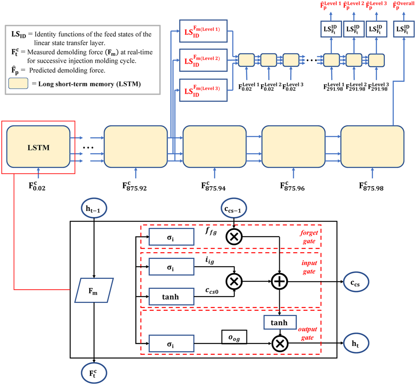
Illustration of the demolding force-LSTM architecture that uses one distinct LSTM per timescale.
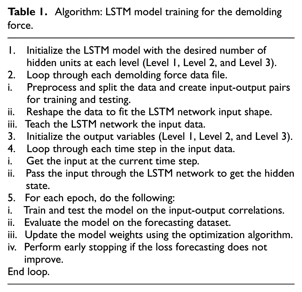
Algorithm: LSTM model training for the demolding force.
In addition, the logical architecture diagram of LSTM sequence expansion is shown on the left to explain the demolding force-LSTM architecture, which uses one separate LSTM per timescale for the three different levels considered in the experimental investigations. Further, the internal logical relationship diagram of a single LSTM is shown on the right; it includes the forget gate
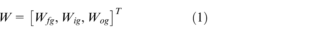
where

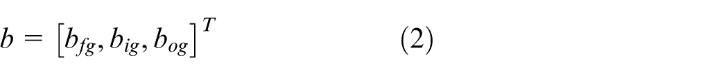
where
The second step is the input gate, which selects what data should be stored in the current time-step. The sigmoid and tanh layers implement this step. As indicated in Eq. (4), the sigmoid algorithm optimizes to update the information. In addition, the tanh layer generates a new cell value and adds it to the cell state (see Eq. (5)).


After these steps, the state

where
The third step is the output gate, which is determined by the sigmoid layer that is run to decide the parts of the cell state going to the output, as expressed in Eq. (7).


where
It should be noted that the dataset was partitioned chronologically in accordance with time-series forecasting principles, ensuring that temporal order was maintained and future data did not influence model training. In addition, to ensure reliable forecasting, data pre-processing steps such as normalization, outlier removal, and smoothing were applied, preserving temporal structure and reducing measurement noise. These procedures enhanced the LSTM model’s ability to capture meaningful patterns and improved generalization across different cycles.
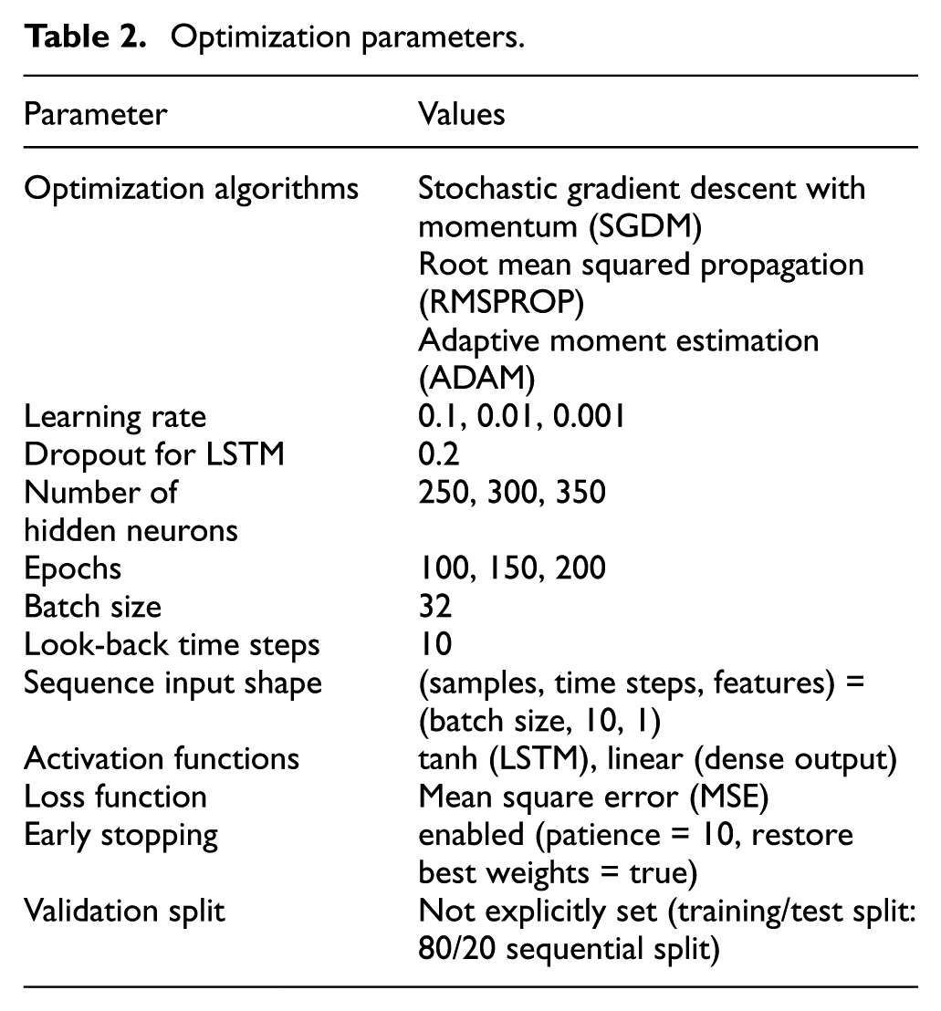
In this study, three gradient descent optimization techniques are used to dynamically improve the weights of the LSTM model to minimize the loss 42 : stochastic gradient descent with momentum (SGDM), 43 root mean squared propagation (RMSPROP), 44 and adaptive moment estimation (ADAM). 45 SGDM serves as a benchmark optimizer, RMSPROP stabilizes learning for non-stationary data, and ADAM provides rapid convergence with adaptive learning rates. This combination allows a balanced evaluation of optimization strategies depending on the model and dataset characteristics. The practical approach is to test a variety of optimizers and select the one that offers the most consistent performance,42,46,47 as shown in Table 2. Furthermore, before implementing the LSTM model, the dataset was diagnostically evaluated using the augmented Dickey–Fuller (ADF) unit root test 48 and normalized between 0 and 1. 49 To obtain the prediction results, the model was denormalized into its original form after training. In addition, the LSTM model’s performance was evaluated using the mean absolute error (MAE),50,51 root mean square error (RMSE) 52 and coefficient of determination (R2).40,53 These metrics capture average prediction error (MAE), sensitivity to large deviations (RMSE), and overall goodness of fit (R2), providing a balanced assessment of predictive performance. The metrics are calculated as follows:
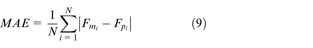
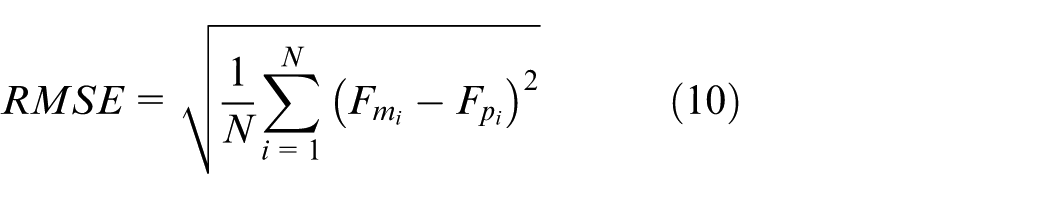
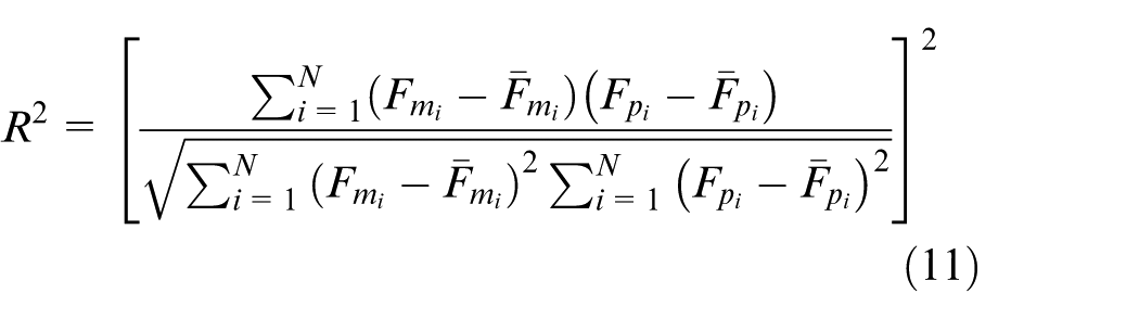
where
Optimization parameters.
Beyond this comparison, the predictive performance of the LSTM model was further evaluated using relative standard regression (RSR), variance accounted for (VAF), prediction index (PI), and likelihood measure of improvement (LMI), as explored in related studies.55–60 These supplementary metrics, detailed in the Supplementary Information, provide a complementary assessment of the reliability of the proposed model. The agreement between the supplementary and primary metrics confirms that the current findings are robust, reproducible, and indicative of the predictive capability of the proposed model.
It should be noted that the LSTM model parameters were determined through empirical tuning, guided by prior studies in deep learning-based time-series forecasting and the specific characteristics of demolding force patterns. Learning rates (0.1, 0.01, 0.001), hidden units (250, 300, 350), and epochs (100, 150, 200) were selected to explore the trade-off between convergence speed, model complexity, and prediction accuracy. A dropout rate of 0.2 was consistently applied to prevent overfitting, and the selected parameter ranges enabled the model to generalize effectively across different experimental levels.
Experimental
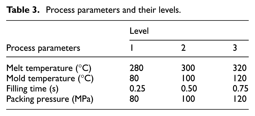
In this study, three different levels of injection molding process were performed using the BOY 25E injection molding machine according to the experimental conditions presented in Table 3 for the used polycarbonate (Infino ML-1020R, LOTTE Chemical Corporation). Three different test levels are employed in the injection molding process to manufacture the designed parts with dimensions of 30 mm × 30 mm × 1.5 mm with a micro slot having dimensions of 10 mm × 0.5 mm × 1.5 mm. During each injection molding process, the demolding force was measured by using a load cell (LCMGD-5 KN, OMEGA) with a measuring range of 0–5,000 N; the load cell was placed behind the ejector rod of the mold core, and the signal was captured using a data logger system (OM-DAQXL-0420, OMEGA), as illustrated in Figure 2. Signals were acquired at a sampling rate of 50 samples per second.
Process parameters and their levels.
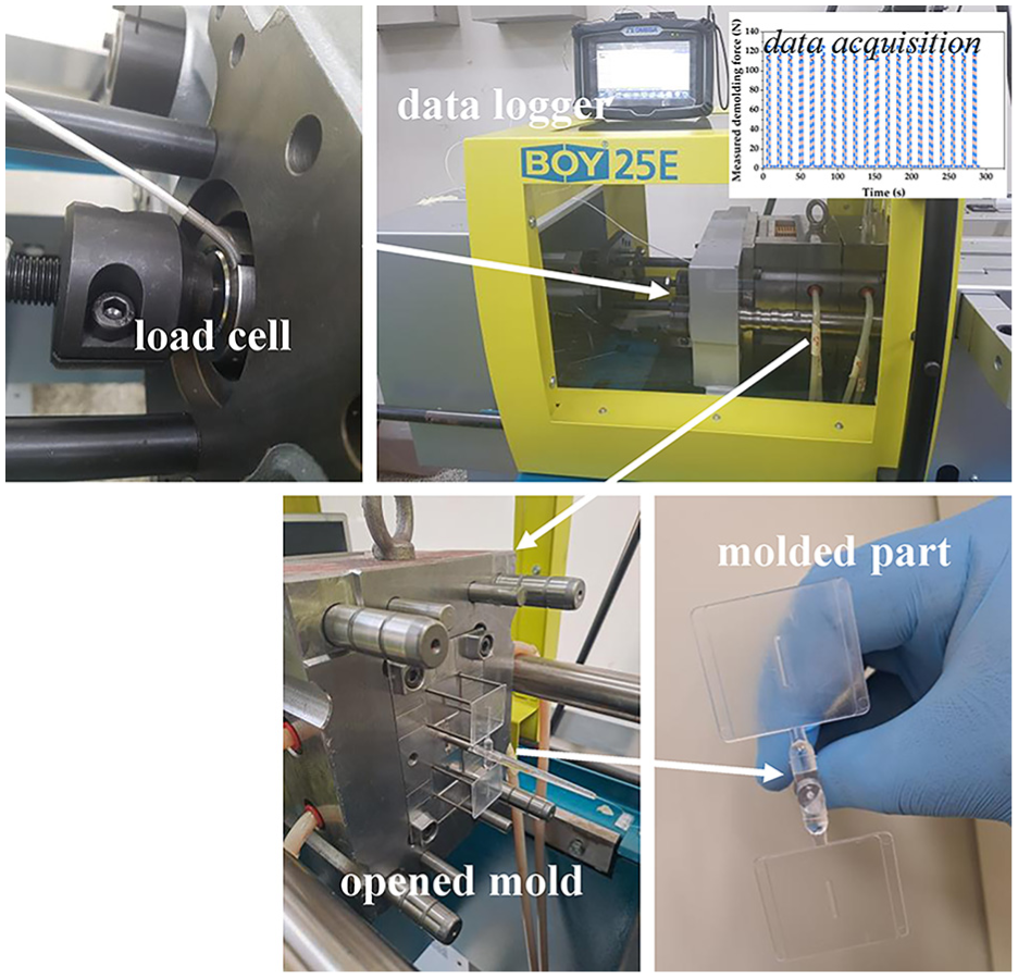
Experimental system to measure the demolding force.
A quasi-experimental design was employed for gathering the dataset in the injection molding experiment. This design technique was used because it allows no manipulation or random assignments for each of the considered cases so as to capture a large dataset during the injection molding cycle.61,62 Each injection molding process performed at different levels to manufacture 20 samples took 291.98 s and returned a large dataset of 14,600 demolding force values. The total dataset of all combined cases contains 43,800 demolding force values at a sampling time of 875.98 s. In general, 80% of the dataset was used to train the forecasting model, and the remaining 20% of the dataset was used for testing the performance of the forecasting model.
The model was implemented in Python 3.9 using Jupyter Notebook (Anaconda3), with Keras (TensorFlow backend) and standard libraries such as NumPy, Pandas, scikit-learn, and Matplotlib for data processing. All model runs were performed on an HP Envy 13 laptop with an Intel Core i7-7500U CPU (2.7 GHz), 8 GB RAM, and a 360 GB SSD running Windows 10. To ensure computational efficiency on limited hardware, a lightweight LSTM architecture was adopted, consisting of a single recurrent layer with a 0.2 dropout rate and early stopping to prevent overfitting.
Results and discussion
To establish the robustness of the demolding force-LSTM model, this section discusses the empirical results of the modeling experiments and the assessments of the performance of the selected optimization algorithms developed to forecast the demolding force at successive injection molding cycles at different time intervals.
Evaluation of model performance
To design the demolding force predictive model, the first step is to deduce whether the demolding force time-series dataset is stationary; the ADF test was used for this purpose. The ADF test is an important diagnostic test in time-series analysis to check for the long-run dynamics of the dataset if it is stationary, and it can efficiently forecast the demolding force. The ADF test, as shown in Figure 3 and Table 4, revealed that a stationarity effect was observed on the demolding force dataset at 1%, 5%, and 10% levels. In addition, it was found that there was no significant change in the test results among three different levels, such as levels 1, 2, and 3. This implies that the current LSTM-based model can provide a reliable prediction regardless of the time-series data obtained under different injection molding conditions.
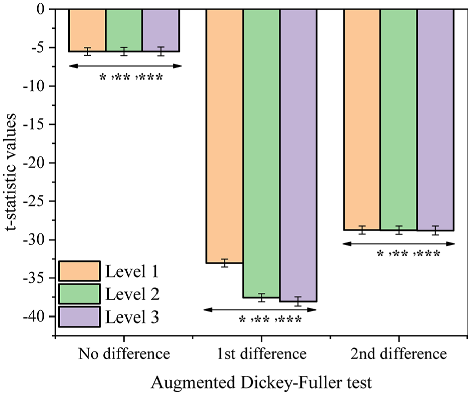
ADF unit root test for the dataset at different levels.
ADF unit root test values for the different levels.
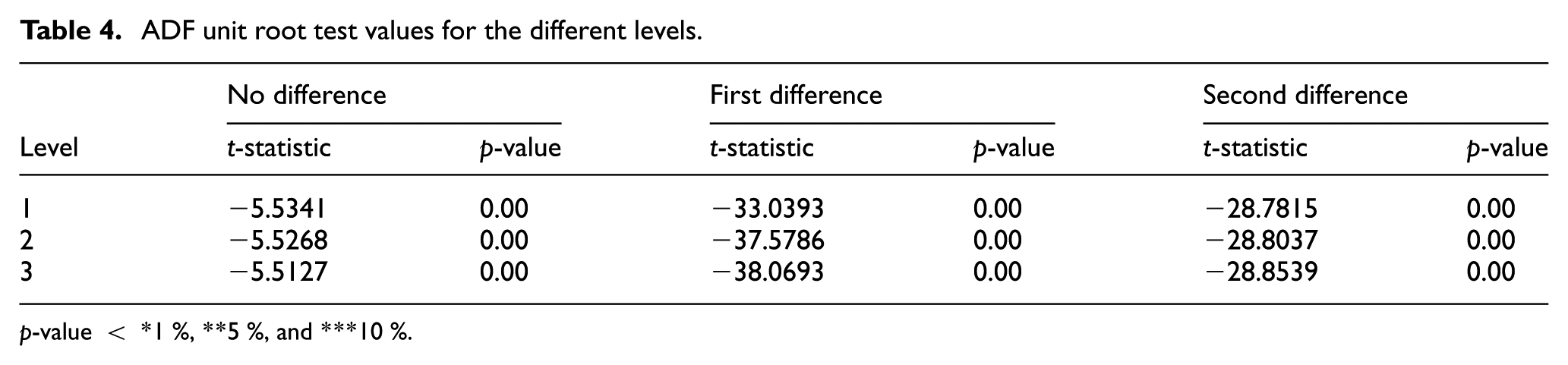
p-value < *1 %, **5 %, and ***10 %.
Having satisfied this condition, the dataset can be analyzed for forecasting. Each modeling optimization algorithm, namely, SGDM, RMSPROP, and ADAM, is performed at three different levels in the experimental injection molding process. To demonstrate the importance of the optimization algorithms over both short- and long-term forecasts in the injection molding cycle, the developed model is evaluated for demolding force prediction series of levels 1, 2, and 3 by using the MAE, RMSE and R2, as shown in Figures 4 –6, respectively. The dataset at each level could seemingly be trained almost perfectly, in that the RMSE values were very small and R2 values were very high at each level in the training stages. Although the time-series datasets obtained from the injection molding experiments were chaotic and noisy, the current models were found to be reliable and accurate in predicting the demolding force.
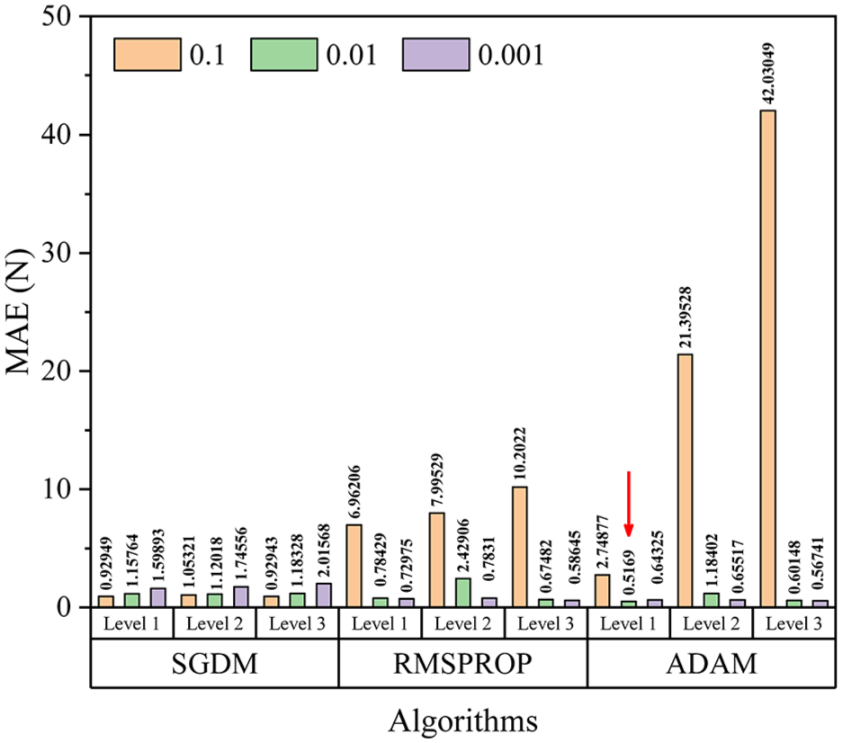
MAE values of the optimization algorithms at different levels and learning rates of 0.1, 0.01, and 0.001.
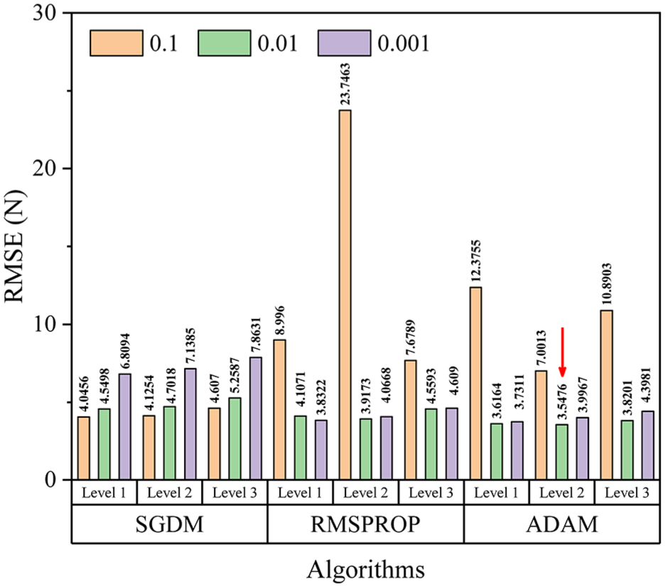
RMSE values of the optimization algorithms at different levels and learning rates of 0.1, 0.01, and 0.001.
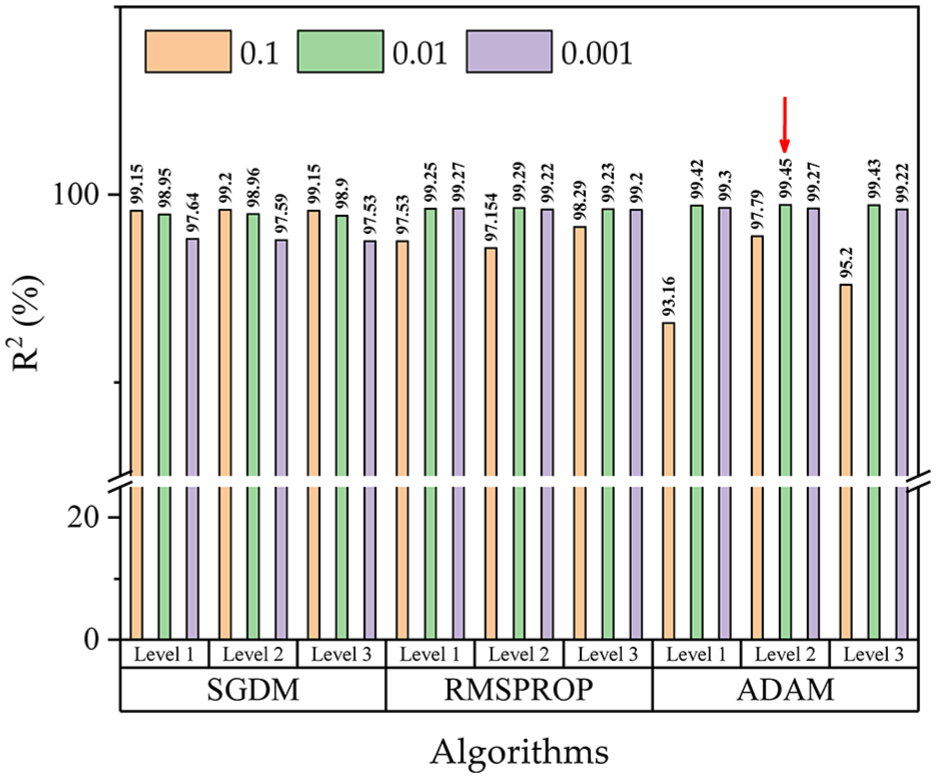
R 2 values of the optimization algorithms at different levels and learning rates of 0.1, 0.01, and 0.001.
To evaluate the stability and consistency of the model across different optimization strategies, the RMSE and MAE plots were analyzed for each level. The LSTM-ADAM configuration yielded the lowest RMSE of 3.5476 N at Level 2, indicating that its predictions closely matched the actual demolding force values with minimal deviation. Additionally, it achieved the lowest MAE of 0.5169 N at Level 1, reflecting the model’s ability to maintain low average error despite minor fluctuations. The gap between RMSE and MAE values across levels suggests that Level 2 contained some small but sharp error peaks, whereas Level 1 exhibited consistently low and stable errors. These results demonstrate that the ADAM-optimized LSTM model is capable of both accurate and robust prediction under varying process conditions.
In addition, the errors of the optimized algorithms at each level varied as seen in Figure 7; this can be caused by the noise effect during the data acquisition of the demolding force in the injection molding process. The results show that the ADAM optimization algorithm performs better than the SGDM and RMSPROP optimization algorithms at level 2. To provide a more comprehensive evaluation of predictive performance, supplementary analyses using RSR, VAF, PI, and LMI were also performed, and the results are documented in the Supplementary Information.
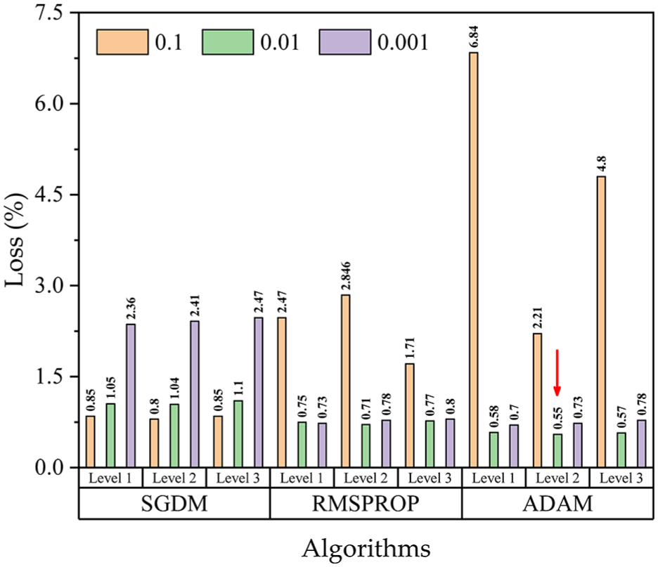
Loss values of the optimization algorithms at different levels and learning rates of 0.1, 0.01, and 0.001.
Evaluation of model reliability
According to the demolding force prediction results of the three different levels shown in Figures 4 –7, the ADAM optimization algorithm is superior compared to the other optimization algorithms in that it has the lowest MAE and RMSE, higher R2, and smaller error values. The ADAM predictive optimization algorithm was evaluated carefully by checking its performance against the actual predicted demolding force and its standard error of the mean demolding force. Figure 8 illustrates these results for predicting levels where a closer examination can be made by a curve fitting performed between the observed and the predicted demolding force over successive injection molding cycles. The ADAM optimization algorithm clearly provides a perfect fit between the measured and predicted demolding force with a relatively small standard error not exceeding 1 N. Importantly, the results show that the ADAM optimization algorithm can generate predicted demolding force values that are very close to the measured values. The prediction efficiency of the ADAM algorithm indicates its potential utility for demolding force monitoring and forecasting in the injection molding process. The application of the ADAM algorithm is immensely useful in the forecasting of the demolding force, where key decisions around the injection molding process at the demolding stage need to be understood ahead of time.
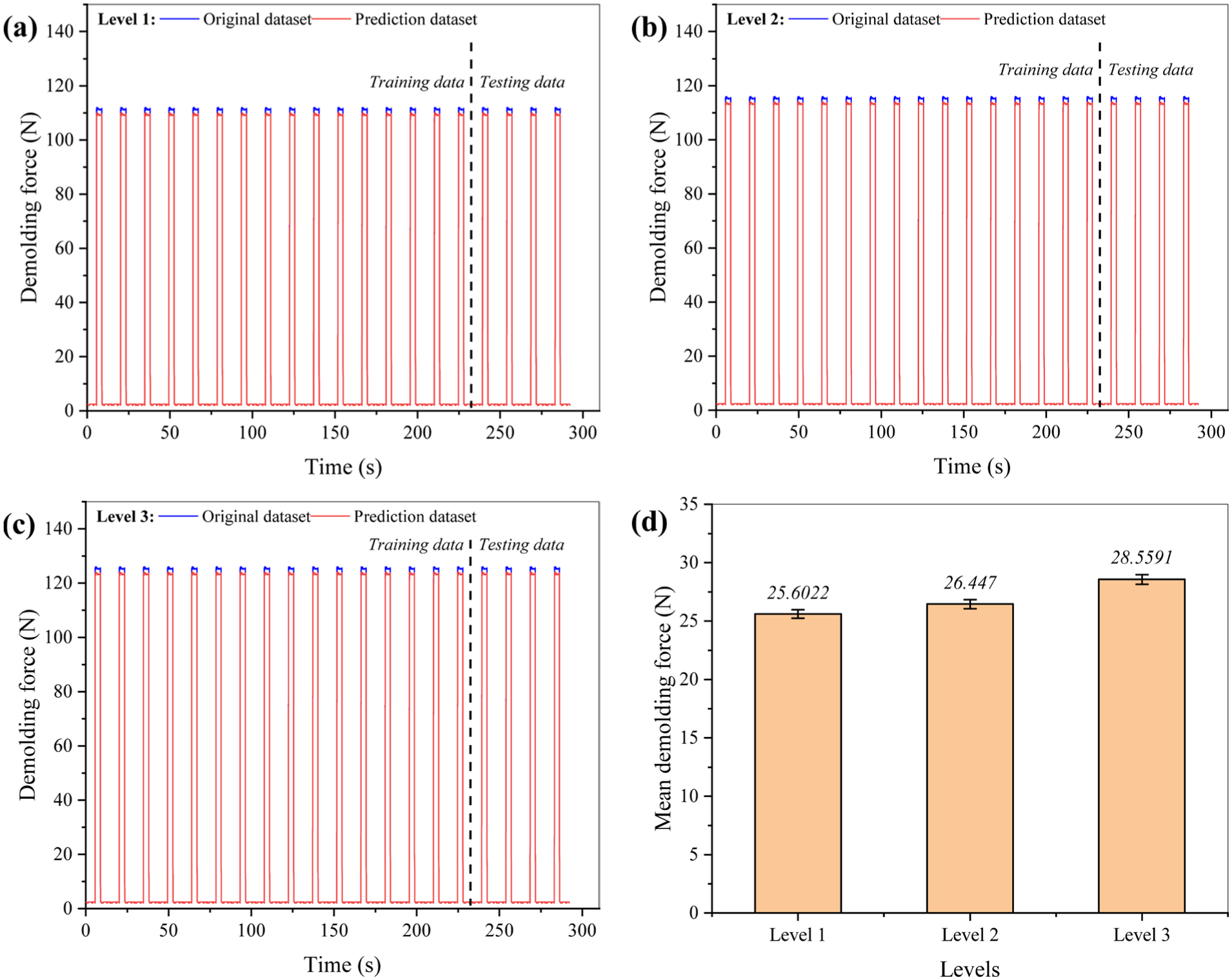
ADAM-LSTM prediction plots: (a), (b), (c) respective model, and the mean demolding force with standard errors (d), at different levels of the injection molding cycle.
Impact assessment of input combination on model performance
This study examined the length of the time-series input sequence and identified the impact of the length of the dataset of the combined levels on the employed ADAM optimization algorithm. The employed algorithm was validated over a long time-period to forecast the demolding force over 18 successive injection molding cycles for a time-series period of
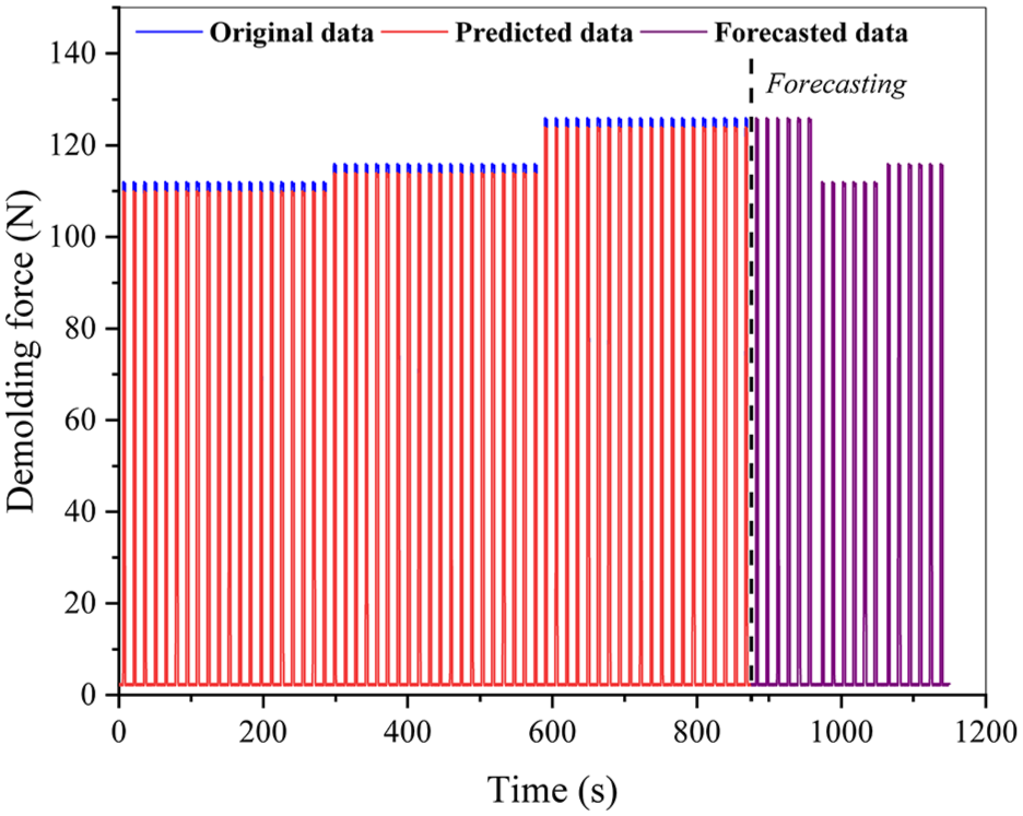
Forecasting results of combined dataset for the demolding force of the injection molding process.
Model validation and comparative performance analysis
Figure 10 presents a validation plot demonstrating the reliability of the LSTM model across various experimental conditions. It compares actual demolding force profiles with predictions from multiple LSTM configurations (LSTM1–3) and ARIMA models (ARIMA1–3) over the injection molding cycles. The periodic spikes in the true demolding force reflect the cyclical nature of the process, which requires accurate modeling of real-time mechanical behavior during mold release.
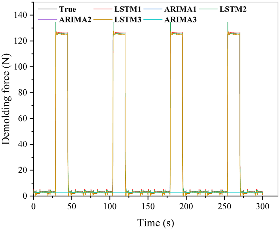
Validation of the combined dataset of the demolding force for four cycles.
Among the tested models, LSTM configurations achieved the highest accuracy, closely matching the measured data. Notably, LSTM1 and LSTM3 showed excellent temporal fidelity, with minimal phase lag and amplitude distortion, indicating the model’s ability to capture complex, nonlinear, time-dependent patterns essential for real-time prediction in dynamic environments. In contrast, ARIMA models failed to capture rapid fluctuations and peak intensities, especially during sudden force surges, revealing the limitations of linear approaches in modeling the nonlinear dynamics of injection molding.
The LSTM’s recurrent architecture enables it to retain long-term dependencies, while dropout and early stopping during training helped prevent overfitting and improve generalization. Overall, the validation plot supports the RMSE and MAE results, confirming that the LSTM model, particularly when optimized with ADAM, can reliably predict demolding force evolution, making it suitable for real-time monitoring and control in industrial applications.
Conclusion
The present study developed and evaluated an ADAM-LSTM time-step model for real-time prediction of demolding force in the injection molding process. Unlike traditional models that require a wide range of process parameters, the proposed model relies solely on real-time measurement data, enabling efficient and streamlined deployment. The LSTM architecture successfully captured long-term dependencies in sequential time-series data, and the ADAM optimization algorithm achieved superior performance in terms of convergence speed, prediction accuracy (low RMSE and high R2), and robustness against overfitting, particularly under level 2 experimental conditions. The model demonstrated its effectiveness in capturing the nonlinear and cyclical nature of demolding force evolution. Notably, the ADAM-LSTM configuration outperformed SGDM and RMSPROP in both predictive accuracy and training efficiency. This performance advantage is attributed to the recursive nature of the LSTM unit, which maintains temporal continuity by feeding outputs from previous time steps into future predictions.
Some limitations remain as the model is sensitive to hyperparameter choices and the dataset was limited to three process levels. Nevertheless, the ADAM-LSTM framework provides accurate, robust forecasting without manual parameter tuning, supporting industrial applications such as predictive maintenance and mold protection. Future work should expand to larger datasets, explore hybrid models, and consider real-time deployment for enhanced industrial applicability.
Supplemental Material
sj-pdf-1-mac-10.1177_00202940251383644 – Supplemental material for Time-series forecasting of demolding force in plastic injection molding using long short-term memory architecture
Supplemental material, sj-pdf-1-mac-10.1177_00202940251383644 for Time-series forecasting of demolding force in plastic injection molding using long short-term memory architecture by Oluwole Abiodun Raimi and Bong-Kee Lee in Measurement and Control
Footnotes
Funding
The authors disclosed receipt of the following financial support for the research, authorship, and/or publication of this article: This work was supported by the National Research Foundation of Korea (NRF) grant funded by the Korea government (MSIT) (No. RS-2024-00357288).
Declaration of conflicting interests
The authors declared no potential conflicts of interest with respect to the research, authorship, and/or publication of this article.
Data availability statement
The dataset for this study will be provided at reasonable request from the corresponding author.
Supplemental material
Supplemental material for this article is available online.
References
Supplementary Material
Please find the following supplemental material available below.
For Open Access articles published under a Creative Commons License, all supplemental material carries the same license as the article it is associated with.
For non-Open Access articles published, all supplemental material carries a non-exclusive license, and permission requests for re-use of supplemental material or any part of supplemental material shall be sent directly to the copyright owner as specified in the copyright notice associated with the article.