
Abstract
Fault diagnosis plays a crucial role in monitoring and maintaining industrial processes and equipment such as discovering solenoid valve faults. Given the intricate nature of complex industrial processes characterized by nonlinearity and dynamics, this paper introduces a novel Temporal-Attention Graph Long Short-Term Memory (TA-GraphLSTM) model for fault diagnosis, which smoothly integrates a hybrid GraphLSTM network module with a temporal-attention block. The novel architecture leverages the strengths of both graph and LSTM neural networks to effectively handle the complexities inherent in industrial data. To construct the input graph structure data, we develop a variable correlation analysis strategy based on the Maximum Information Coefficient (MIC), which facilitates accurate representation of the relationships between variables. Furthermore, the incorporation of the temporal-attention module allows the model to dynamically assign weights to hidden variables across time steps to capture temporal dependencies effectively. The proposed TA-GraphLSTM fault diagnosis method is validated through the application of a spacecraft propulsion system. The experiment results prove the effectiveness and robustness of the model.
Keywords
Introduction
It is crucial to monitor industrial processes to ensure the safety and reliability. When abnormal condition is detected, it is also urgent to identify the root cause of the problem. Therefore, process monitoring and fault diagnosis play an important role in the stable operation of industrial systems.1–4 Due to the complexity of modern industrial processes, accurate mathematical models are often difficult to establish, therefore data-driven approaches are necessary and crucial to capture the underlying characteristics of complicated system. To this end, bunches of data-based process modeling and fault diagnosis models have been developed recent years to meet the demand of diverse industrial scenarios.5,6
With the development of the data collection, transmission and storage technology, process modeling based on machine learning is becoming the mainstream of data-based modeling methods. With abundant data, these methods are capable of extracting hidden features of processes to establish connections between input samples and fault conditions such as principal component analysis (PCA), partial least squares (PLS), canonical correlation analysis (CCA), and support vector machine (SVM) and their variants.7–13 However, due to the increasing scale of industrial processes, the complexity and coupling of processes have become more apparent, and traditional linear modeling and fault diagnosis methods are difficult to achieve ideal results. To address this issue, in recent years process modeling and fault diagnosis algorithms based on deep learning technology have greatly improved the identification performance through more effective feature learning and nonlinear modeling strategies. For example, convolutional neural network (CNN) is one of the most widely-used deep learning techniques for feature learning and fault diagnosis of industrial processes.14–16 It is often combined with signal processing approaches to identify fault conditions of bearing faults and other mechanical failures. CNN automatically learns data features through convolution operations and utilizes the parameter sharing and local connection strategies, which effectively reduces the model parameter and computational complexity. The convolutional kernels can be enhanced with autoencoders (AE) for unauthorized broadcasting identification and the expert knowledge hidden in normal signals can be extracted and emphasized. 17
Graph neural network (GNN) is also an effective nonlinear modeling model based on deep learning, which has been successfully applied on feature extraction and fault diagnosis of numerous fields.18–21 Compared to CNN, GNN updates node representations by aggregating information from neighboring nodes, which can capture complex structures and relationships in graph data. This is crucial for handling datasets with complex interactions and dependencies.
Another important issue of complex industrial process modeling is the time-varying characteristic of data. The temporal correlations between samples are usually ignored using traditional static modeling methods. Therefore, dynamic deep learning modeling frameworks are developed to extract the characteristics of time-series data. For example, recurrent neural network (RNN) is an effective structure. Unlike traditional neural networks such as CNN, RNN is able to process each element in a data sequence and consider the information of the preceding elements in the sequence. 22 This advantage makes RNN particularly suitable for handling tasks where dependencies are important before and after. RNN has been successfully used for process modeling and fault diagnosis. Long short-term memory (LSTM) neural network is a special variant of RNN that has significant advantages over traditional RNNs in processing sequence data. Compared with RNN, LSTM is able to capture long-term dependencies in time-series data by introducing memory units and gating mechanisms.23,24 Therefore, LSTM performs better in handling with long-term memories including complicated systems with strong time correlations. Recent years, LSTM-based modeling methods have been proposed to applied in important tasks such as process modeling, fault detection, quality prediction, and fault diagnosis for complex processes.25–27 For example, combining CNN and LSTM driven by few-shot learning, a real-time transformer discharge pattern recognition task was achieved. 28 Besides, the identification and control of nonlinear systems via deep long short-term memory (DLSTM) networks-based Wiener model (W-DLSTM) was investigated for the permanent magnet synchronous motor (PMSM) system. 29 Together with extreme learning machine (ELM) and Elman neural network (ENN), LSTM was adopted as a part of the first network layer for short-term wind speed prediction. 30 To further improve the modeling accuracy, the attention mechanism is developed as an important technique in machine learning, especially when dealing with sequential data or complex data. The main idea is to enable the model to automatically focus on more important parts during the modeling procedure, thereby improving both the performance and efficiency of models. Li et al. 31 developed an optimal planning strategy of integrated electricity and heat systems based on convolutional neural networks and bidirectional long short-term memory networks with attention mechanism (CNN-BiLSTM-Attention), while better forecasting results and the global optimal solution of the dual objective function can be obtained. Other deep learning strategies were also proposed in recent years. lightweight neural network such as MobileViT and MobileRaT were developed for real-time constellation image classification and automatic Modulation Classification.32,33 A complete ensemble empirical mode decomposition based multi-stream informer (CEEMD-MsI) was proposed to predict the hourly PM2.5 concentration in Shandong, China. 34 A novel three-stage dynamic false data injection attack (DFDIA) model in cyber-physical power system was proposed by considering potential dynamic behaviors, where both attack location and attack amplitude are taken into consideration. 35
In this paper, a deep feature learning method using temporal-attention GraphLSTM model is proposed to implement the fault diagnosis task of solenoid valves in propulsion systems. There are three modules in the proposed model. Two GCN layers are connected as the first module. An adjacency matrix is determined through the feature analysis of raw data. Hence, the input graph structure is constructed referring to the adjacency matrix. By the use of GCNs, both the variable correlations and data nonlinearity can be extracted effectively. Then, an LSTM layer is introduced after a ReLU layer as the second module of the proposed model. As a result, the temporal correlations of data can be analyzed, which is a perfect complementation to the GCN module. To further improve the modeling quality, the weights of the samples along the time indexes are decided through a temporal attention module. Time-series samples that have a greater impact on the fault diagnosis results will be given higher weights during this process. In the proposed fault diagnosis model, a higher weight indicates a stronger correlation between the relevant temporal sample and the model output, which play a more critical role in the diagnosis process. Hence, these weights allow the model to emphasize important time steps such as recent changes and crucial anomalies while irrelevant samples along the time index is ignored. Finally, the type of fault can be well identified, indicating a satisfactory fault diagnosis result. The main contribution of this work is illustrated as follows:
(1) A hybrid fault diagnosis model is developed, which combines the advantages of both GNN and LSTM. In the proposed model, GCNs are developed to extract the variable correlations as well as the nonlinear characters of data, while and LSTM layer is introduced to capture the time-related features of data. By embedding GCN into LSTM, simultaneous modeling of graph-structured data and sequential data can be achieved. Compared to the existing models such as LSTM, CNN-LSTM, it is able to provide better fault diagnosis capability when dealing with complex tasks.
(2) The temporal attention mechanism is adopted in this work, which is able to significantly improve the sequential modeling accuracy. The temporal attention mechanism allows the model to assign different weights to different time steps when processing sequential data. Compared to these models without the temporal attention block, the proposed model focuses on important time steps while allocating less attention to less significant steps. Hence, the model performance and accuracy can be significantly enhanced.
The rest of this paper is organized as follows. Section 2 introduces some preliminaries of related knowledge. Section 3 demonstrates the methodology and its implementation process. Then, the proposed method is testified in a propulsion system to identify the fault types of solenoid valves and other components. In the end, conclusions are drawn.
Preliminaries
Graph Neural Network
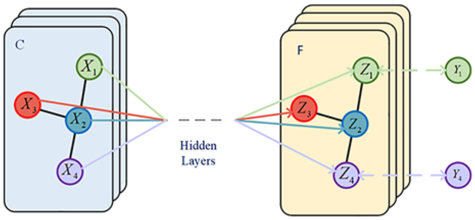
GNN is a deep learning model specifically designed for processing graph structured data. With the rise of complex relational data such as social networks, knowledge graphs, and chemical molecules, GNN has demonstrated powerful capabilities in tasks such as graph analysis, node classification, and link prediction.
Among various GNN models including graph convolutional network (GCN), graph attention network (GAT), graph auto-encoder (GAE), graph generative network (GGN) and other structures, GCN is considered as the most widely-used one. GCN extracts feature representations from graph structured data through convolution operations. The basic input structure of GCN mainly includes two parts, which are an adjacency matrix and the feature matrix of the nodes. GCN mainly performs convolution operations based on spectral decomposition or node space transformation to achieve analysis and processing of graph structured data. It can be denoted as 36 :
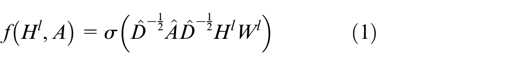
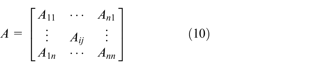
where A is the adjacency matrix representing the connection relationships between nodes in the graph structure, which can be obtained by variable correlation analysis approaches;
Graph convolutional network.
Long short-term memory neural networks
LSTM is a special type of RNNs designed to solve the problems of gradient vanishing and exploding that traditional RNNs face when processing long-sequence data. Compared to traditional RNNs, LSTM ca effectively capturing long-term dependencies. It was first proposed by Hochreiter and has been widely applied in multiple fields through consecutive research and improvement. Due to its powerful sequence modeling capabilities, LSTM has achieved outstanding performance in natural language processing, speech recognition, time-series prediction, and image processing.
LSTM develops gating mechanisms and explicit memory units including forget gate, input gate, and output gate, which collectively control the flow and storage of information. The forget gate controls the degree to which information in the previous memory unit is retained, and outputs a value between 0 and 1 through the sigmoid function. The input gate controls the degree to which the current input information flows into the memory unit, also outputs a value through the sigmoid function, and combines it with a candidate value vector created by a tanh layer to jointly determine the update of the memory unit. The output gate controls the amount of long-term memory output, which determines the information in the memory unit to be outputted to the hidden state at the current time. It can be denoted as 37 :


where,
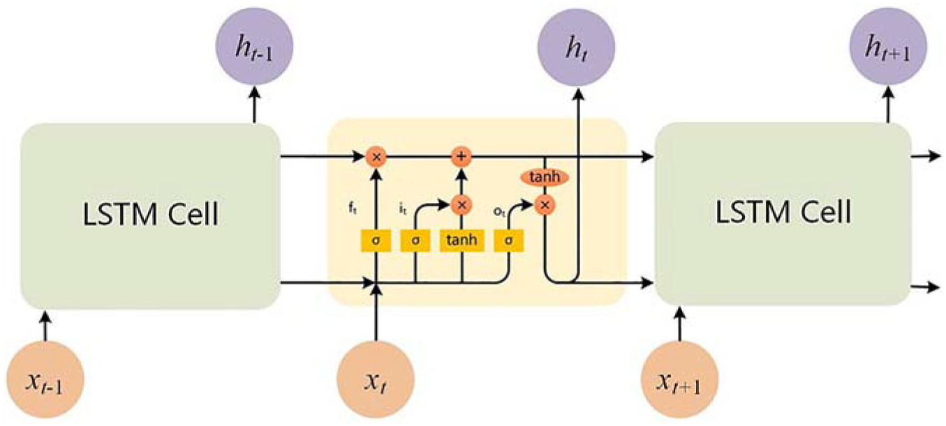
Long short-term memory neural network.
For the specific gate structure, the forget gate
Methodology
In this section, the temporal-attention GraphLSTM (TA-GraphLSTM) model is constructed to deal with the fault diagnosis issue of industrial processes such as the solenoid valve faults in propulsion systems. The detailed structure of the proposed TA-GraphLSTM model is illustrated in Figure 3. The raw data is first subjected to feature analysis to obtain the adjacency matrix. Subsequently, the graph structure between variables is constructed through data transformation to form the input of the model. Next, the data will go through two GCN layers to fully extract local information and nonlinear features of the graph structured data. Subsequently, the output graph data is passed through a ReLU layer and introduced as the input into an LSTM layer to further extract dynamic features from the data. Considering that LSTM cannot reflect the contribution of different time units to the model output in the process of time series modeling, a temporal-attention module is further developed in the model to enable different weights to be obtained for sequential data at different time steps, therefore obtaining a more accurate model. Except for the basic neural network modules illustrated in the previous section, the feature analysis and graph structure construction process will be demonstrated in detail in this section, as well as the development of the temporal-attention module.
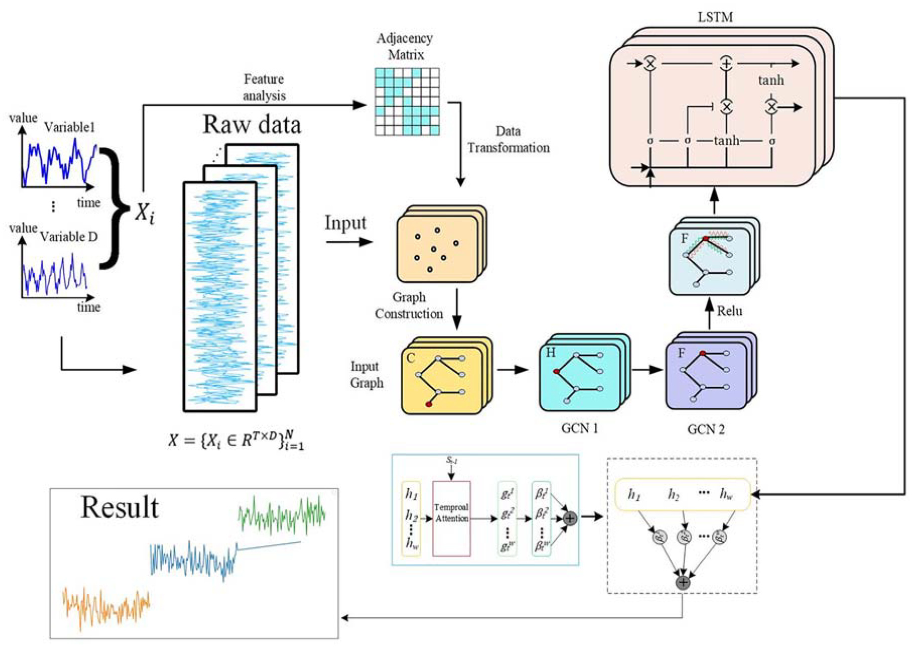
Framework of the proposed temporal-attention GraphLSTM.
Graph Structure Construction
The graph structure of GNNs consists of two parts, which are the adjacency matrix and the node data. The adjacency matrix is a fundamental concept of GNN which represents the node relationship of variables. The edges between nodes are constructed by feature analysis as a critical representation for GNNs to process and propagate information through the graph topology. The adjacency matrix is typically derived from the results of variable correlation analysis.
Common correlation analysis techniques encompass the Spearman’s rank correlation coefficient, the Pearson correlation coefficient, and other correlation coefficient methods. Nevertheless, these techniques are primarily tailored for linear data or nonlinear data exhibiting straightforward monotonic relationships. Alternatively, methods like Kernel Density Estimation (KDE) and K-nearest neighbors (KNN) are more adept at handling nonlinear data. However, these nonlinear methods present challenges in terms of high computational complexity and robustness.
The maximum information coefficient (MIC) is a typical feature extraction and variable correlation analysis technique. It aims to measure the correlation between two variables, which is advantageous when dealing with data featuring complex relationships. Consequently, we have opted for MIC as our correlation analysis method, as it is better equipped to address the complexities inherent in industrial data with lower computational complexity. Given two process variables
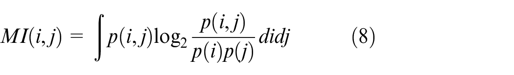
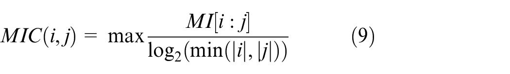
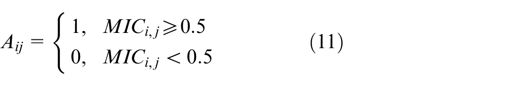
Therefore, a higher MIC indicates a more significant correlation between these two variables. In order to clarify the composition of the graph structure and determine the relationship between nodes and edges in the graph structure data, the method for determining the values of adjacency matrix elements is fixed in this work. When the MIC is greater than or equal to 0.5, the corresponding element value of the adjacency matrix is set to 1, while the corresponding matrix element value is assigned to 0 under the condition that MIC is less than 0.5. Therefore, the adjacency matrix can be obtained as:
Fault diagnosis model based on TA-graphLSTM
With the adjacency matrix A, the node data can be represented as
After defining the graph structure, the graph data is first processed through the GCN layers. A degree matrix
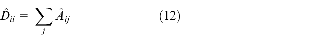
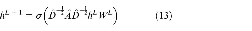
where
Then, a temporal attention module is developed to further capture time-relevant characteristics of data. The attention mechanism is an important concept derived from the study of human vision, which simulates the ability of humans to selectively focus on and prioritize important information when processing large amounts of information. In the fields of artificial intelligence and deep learning, attention mechanisms are widely applied in various tasks, especially in the areas of natural language processing and computer vision. The core idea of the attention mechanism is to calculate the importance of different parts of input data to the current task and assign different weights to these parts, thereby achieving efficient information processing results.
The temporal attention mechanism automatically learns the weights associated with different time steps in the sequence, allowing it to focus on the most critical time step information for the task. Specifically, it first transforms the features of each time step into a new representation space using specific layers. Then, it computes the attention weights for each time step and highlights their relative importance to the output. Finally, the attention weights are determined and averaged with the mapped features to obtain the final temporal representation. In this work, a query vector


where

where
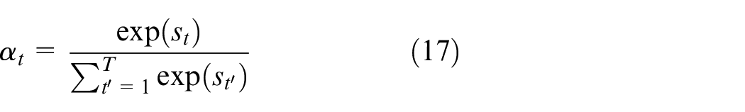
Therefore, time steps with higher attention weights
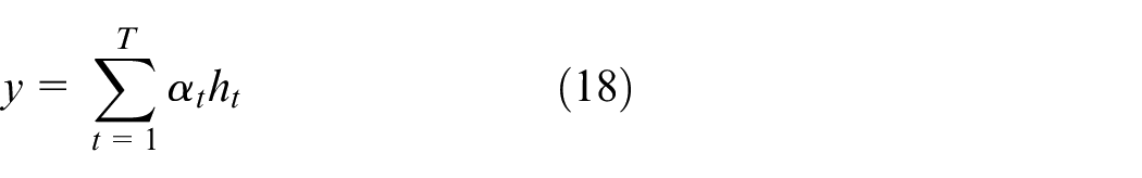
In equation (18), the model output
Fault diagnosis implementation
The flowchart of the TA-GraphLSTM based fault diagnosis method is shown in Figure 4.
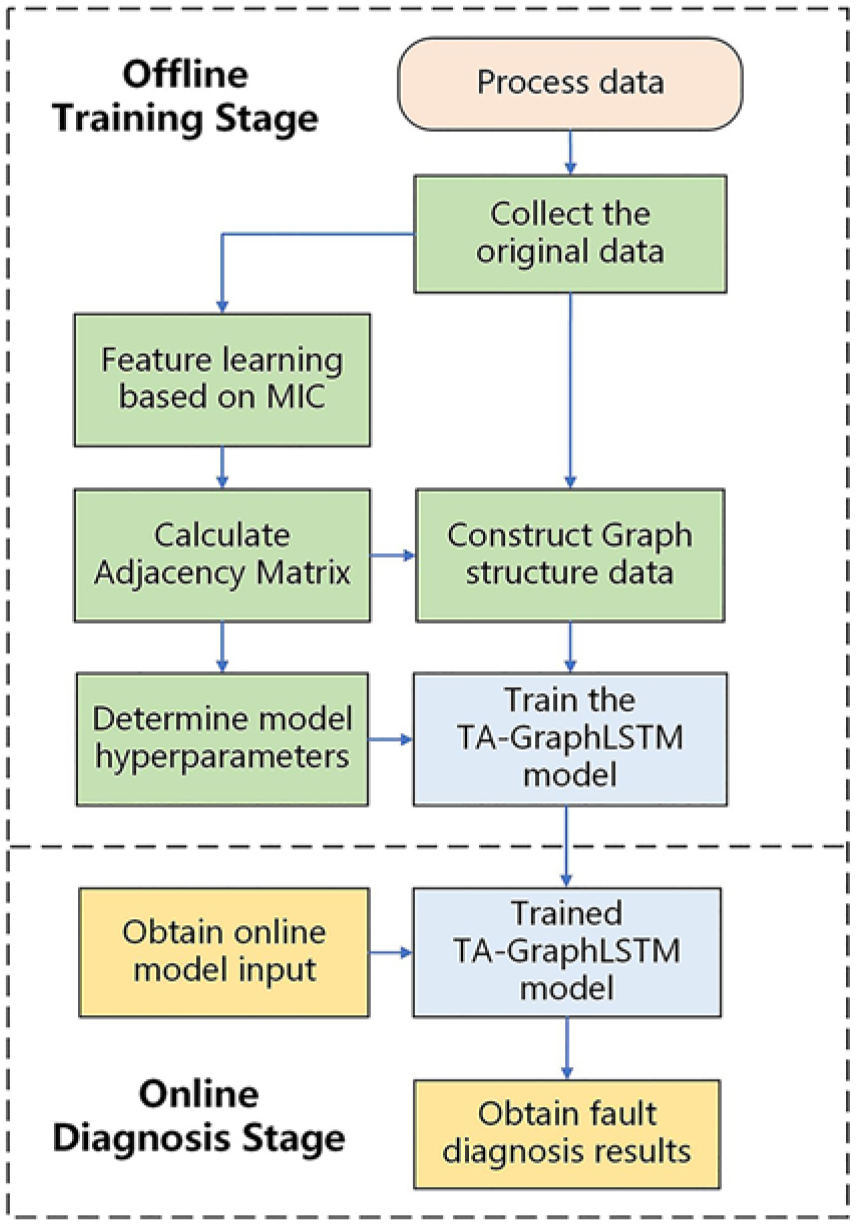
Flowchart of the TA-GraphLSTM based fault diagnosis method.
The main steps of the proposed method are also presented as follows.
(1) Collect enough process data including state variables as the model input and fault type as the output;
(2) Implement feature learning on input variables based on the maximum information coefficient strategy;
(3) Determine the adjacency matrix according to the calculation results of maximum information coefficient;
(4) Construct the graph structure data referring to the adjacency matrix as the input of the TA-GraphLSTM model;
(5) Determine the model hyperparameters and train the TA-GraphLSTM fault diagnosis model;
(6) Collect the online samples and fed into the trained TA-GraphLSTM model;
(7) Obtain the model output as the fault diagnosis result of the current input.
Experiments
In this section, a case study on a spacecraft propulsion system is conducted to evaluate the effectiveness of the proposed TA-GraphLSTM fault diagnosis model, which is a case of the data challenge in 2023 Prognostics and Health Management Asia-Pacific Conference (PHMAP23). Figure 5 presents the experimental setup of the propulsion system, where water serves as the working fluid, pressurized to 2 MPa and subsequently discharged through four solenoid valves (SV1–SV4), effectively mimicking the operation of thrusters. Embedded within the system are several pressure sensors labeled as P1–P7, which facilitate the acquisition of time-series data at a precise sampling rate of 1 kHz, spanning a duration of 0–1200 ms. By strategically manipulating the opening and closing of the solenoid valves, the resultant pressure fluctuations can be observed.
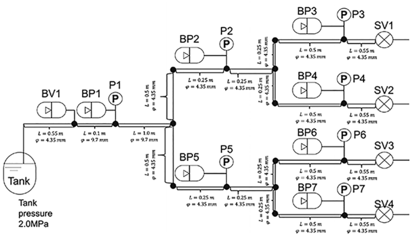
Schematic of the propulsion system.
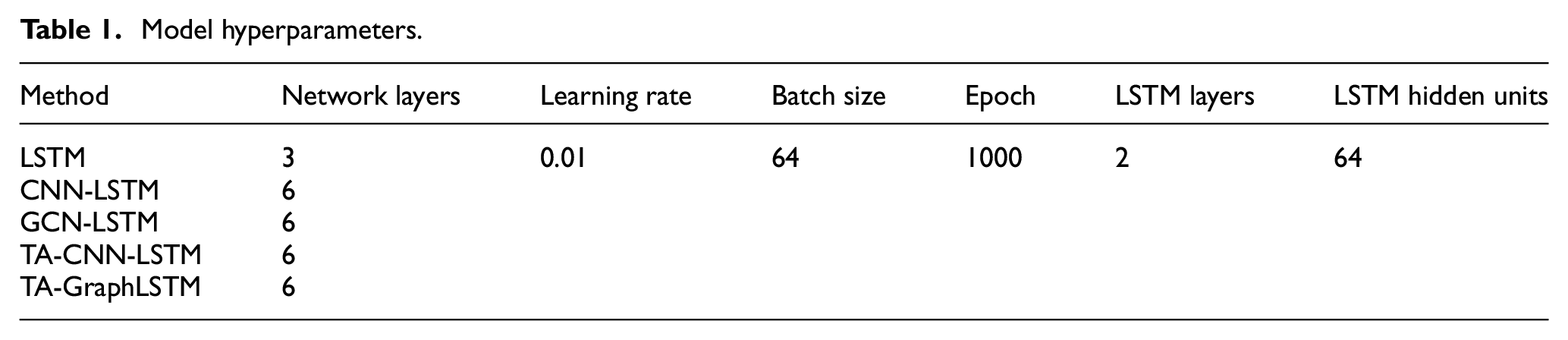
In this experiment, two distinct types of abnormal conditions are taken into consideration: the abnormal opening of the solenoid valves and the bubble contamination. The solenoid valve fault is the major failure mode of the propulsion system. In this case of faults, the solenoid valves may open to varying degrees, ranging from 0% to 100%, leading to a consequential reduction in the volume of water passing through the valve. This reduced flow can significantly impact the overall performance and efficiency of the propulsion system. The detection and diagnosis of solenoid valve faults are necessary since it is urgent to locate the abnormal solenoid valve to prevent further failure and damage. Besides, during the actual operation of spacecraft, bubbles occasionally appear in the pipelines. The presence of bubbles changes the speed of sound, causing small changes in pressure fluctuations. Hence, the appearance of bubbles should be detected and the location need to be diagnosed. There are seven measuring points in the system, which are pressure sensors as aforementioned. The training dataset contains 177 training cases, where 105 of them are normal cases, 48 are solenoid valve fault cases and 24 are bubble anomalies. To prove the effectiveness of the proposed TA-GraphLSTM model, several fault diagnosis models are adopted to the comparative experiments including LSTM, CNN-LSTM, GCN-LSTM, temporal-attention CNN-LSTM (TA-CNN-LSTM). The hyperparameters of these models are listed in Table 1, which are determined by the trial-and-error strategy. The experiments are carried out on a high-performance workstation equipped with an Intel Core i9-13900K CPU operating at a base frequency of 3 GHz, complemented by 128 GB of RAM and a NVIDIA GeForce RTX 4090 graphics card with 24 GB memory. Python and Spyder are utilized to execute the code.
Model hyperparameters.
To prove the effectiveness of the proposed TA-GraphLSTM fault diagnosis model, 20 normal cases and 20 fault cases including solenoid faults and bubble anomalies are adopted as the testing dataset, while each case has 1200 samples. Therefore, totally 48,000 samples were tested, by which the generalization ability and robustness of the model can be evaluated. The fault diagnosis results are shown in Figure 6.
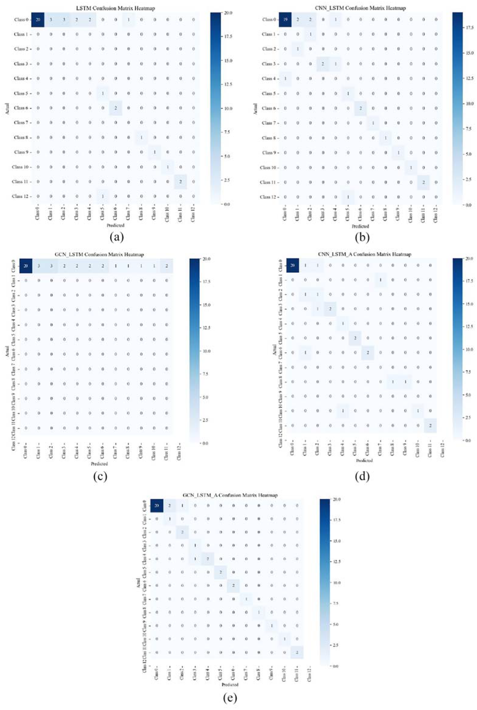
Fault diagnosis results: (a) LSTM, (b) CNN-LSTM, (c) GNN-LSTM, (d) TA-CNN-LSTM, and (e) TA-GraphLSTM.
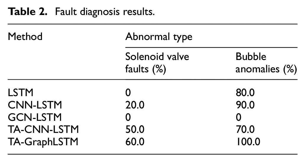
The diagnosis accuracy of each method for different types of abnormal conditions is demonstrated in Table 2. Meanwhile, the mean accuracy of all conditions including the normal condition is presented in Figure 7.
Fault diagnosis results.
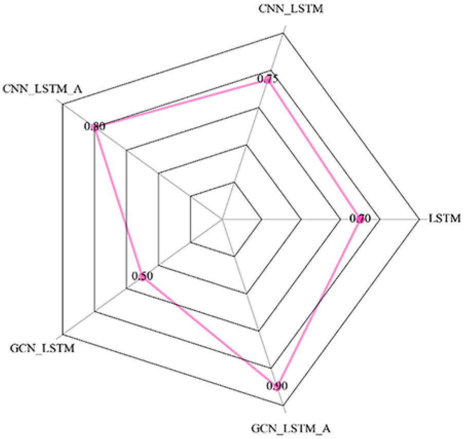
Radar chart of the total diagnosis accuracy.
From the results of the comparative experiment, it can be clearly inferred that the TA-proposed GraphLSTM fault diagnosis model has achieved the best performance in diagnosing different types of abnormal conditions as well as the overall diagnostic accuracy including normal conditions compared to other methods. Although LSTM can extract dynamic features of data, it lacks sufficient analysis of local features and correlations of variables, resulting in unsatisfactory fault diagnosis results. After combining with CNN, the hybrid fault diagnosis model based on CNN-LSTM improves the performance of the fault diagnosis model through local modeling and feature extraction. Hence, after compared with the simple LSTM model, the diagnostic effect is slightly improved. Similarly, after attempting to construct a hybrid model in combination with GCN, the improvement was not significant in terms of results. It is worth noting that the performance of the fault diagnosis model has been significantly improved after adding the temporal-attention module. It can be seen that after combining attention mechanism, the fault diagnosis accuracy of CNN-LSTM model is improved by up to 5%. At the same time, the TA-GraphLSTM model proposed in this paper has greatly improved the accuracy of diagnosis by introducing both temporal-attention modules and hybrid GNN models, and has become the best approach among all these methods reaching 90.0%.
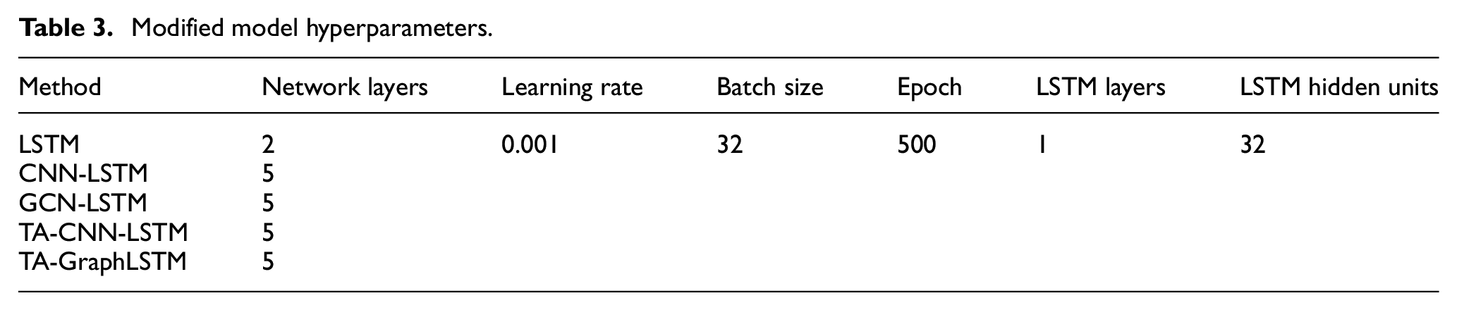
To further analyze the factors affecting model performance such as model parameters, we have conducted experiments based on another set of model hyperparameters as shown in Table 3.
Modified model hyperparameters.
The fault diagnosis results based on confusion matrix heatmaps with the new set of model hyperparameters are shown in Figure 8.
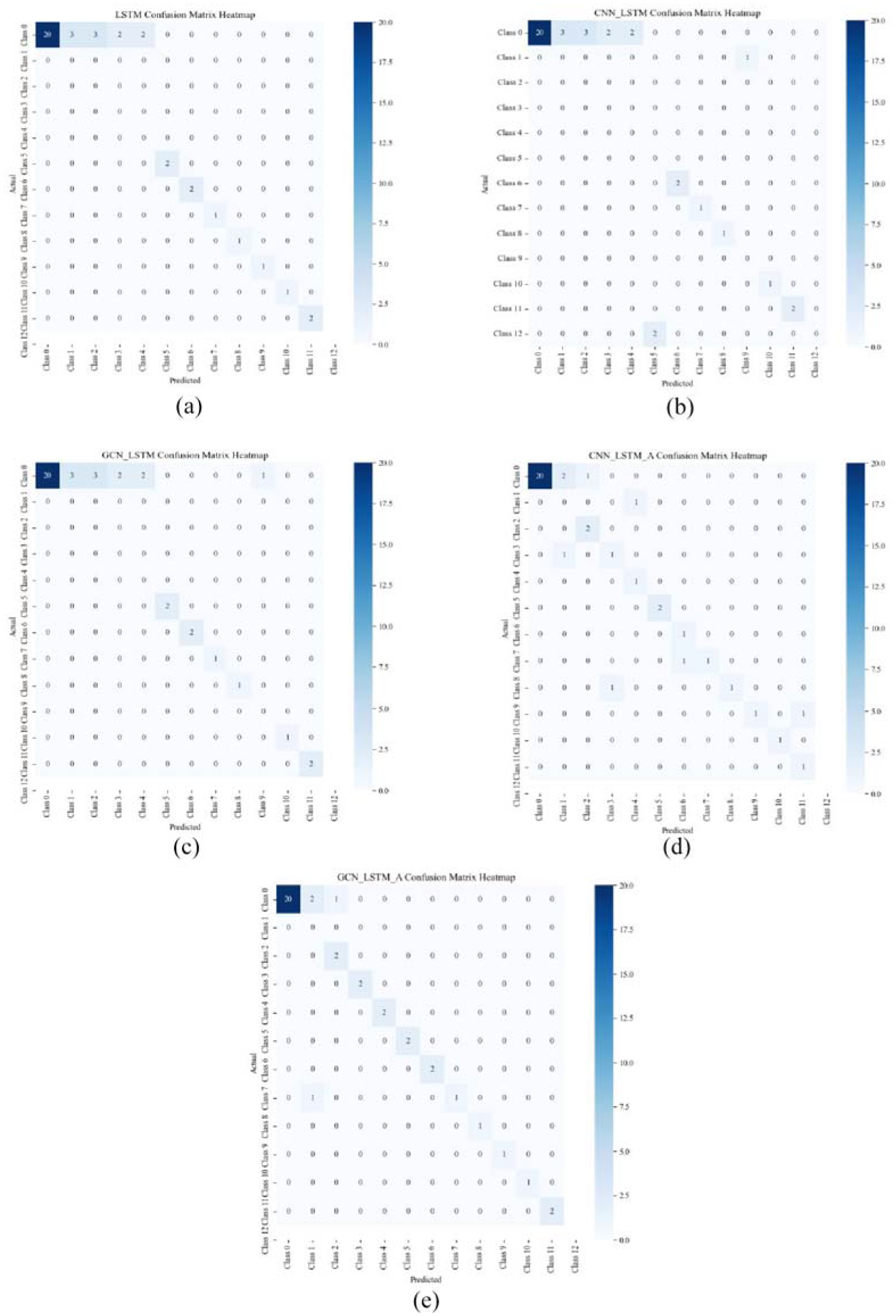
Fault diagnosis results with modified model hyperparameters: (a) LSTM, (b) CNN-LSTM, (c) GNN-LSTM, (d) TA-CNN-LSTM, and (e) TA-GraphLSTM.
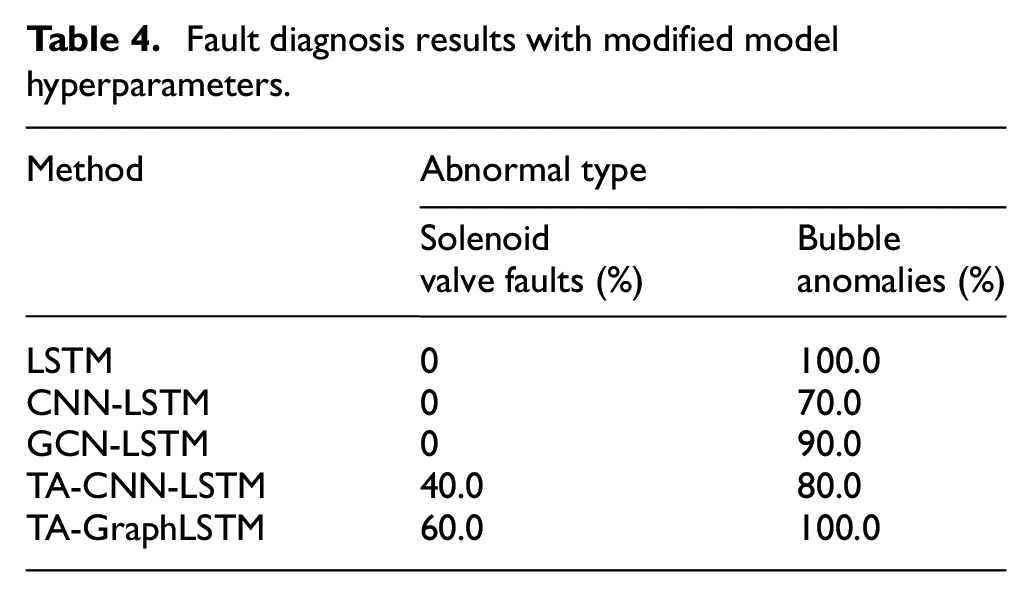
Meanwhile, the diagnosis accuracy of each method with the new set of model hyperparameters for different types of abnormal conditions is demonstrated in Table 4. The mean accuracy of all conditions including the normal condition is also presented in Figure 9.
Fault diagnosis results with modified model hyperparameters.
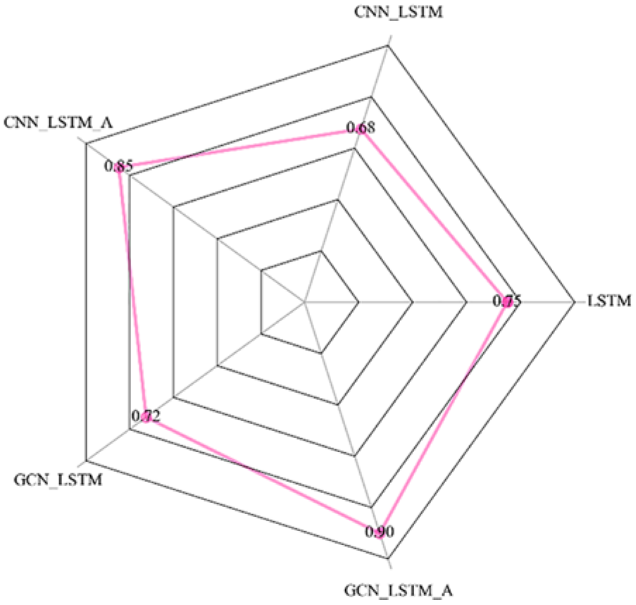
Radar chart of the total diagnosis accuracy with modified model hyperparameters.
It can be inferred from the diagnosis results with modified model hyperparameters that the proposed TA- GraphLSTM model keeps the best diagnosis accuracy among all the methods, while other methods reflect a certain degree of fluctuations. The results demonstrate that the proposed model possesses both high accuracy and strong robustness.
Conclusions
This paper proposes a temporal-attention GraphLSTM fault diagnosis model. Simultaneous modeling of both graph data and time-series data can be achieved by the hybrid network structure, while these time steps with more contribution to the model output can be automatically identified. This model mainly consists of two parts, which are the hybrid GNN module and the temporal-attention module. In the hybrid graph neural network part, a hybrid network structure is constructed by combining GCN and LSTM networks, which preserves both the excellent interpretability and local feature extraction ability of GCN, as well as the strong feature extraction ability of LSTM for time-series data. By designing a variable correlation analysis method based on maximum information coefficient, the input graph structure data can be effectively constructed. In the temporal-attention module, different weights are assigned to hidden variables at different time steps. Therefore, the fault diagnosis model becomes more sensitive and accurate to temporal correlations. The proposed method has successfully been applied to the fault diagnosis problem of a spacecraft propulsion system. Comparative experiments prove the effectiveness of the proposed method.
Future work will focus on hyperparameter optimization, model generalization ability improvement, and more scenario applications. Implementing automated hyperparameter optimization and adaptive graph construction can significantly enhance the model performance. Meanwhile, developing domain adaptation and cross-validation strategies will help the diagnosis model perform better on unseen data. Finally, the fault diagnosis method proposed in this paper will be further studied and applied to more diverse industrial scenarios such as power systems and chemical processes.
Footnotes
Declaration of conflicting interests
The author(s) declared no potential conflicts of interest with respect to the research, authorship, and/or publication of this article.
Funding
The author(s) disclosed receipt of the following financial support for the research, authorship, and/or publication of this article: This research was supported by the China Postdoctoral Science Foundation [grant number 2023M730649], the National Natural Science Foundation of China [grant number 62103360, 62373147], the Zhejiang Provincial Natural Science Foundation of China [grant number LTGG23F030002], the Ningbo Natural Science Foundation [grant number 2024J023], and the Key Research and Development Program of Ningbo [grant number 2022Z165, 2024T011].
Ethical considerations
Not applicable.
Consent to participate
Not applicable.
Consent for publication
Not applicable.
Data availability
Data associate with the paper is available upon requests to the corresponding author.