
Abstract
Long-term operation of electric motor under complex and extreme conditions can lead to unpredictable failures, therefore, accurate diagnosis of electric motor failures has been valued by scholars and engineers. However, the noise in the vibration signals of the motor’s rolling bearings has a profound impact on the diagnostic performance of a model in the process of feature extraction and fault classification. Aiming at vibration signal denoising and accurate fault classification, in this study, a novel method based on WOA-SVMD and multi-scale CNN-Transformer is proposed. Firstly, the Whale Optimization Algorithm (WOA) is employed to obtain the optimal parameters of Successive Variational Mode Decomposition (SVMD), which is then used to decompose the signal into Intrinsic Mode Functions (IMFs). Secondly, uncorrelated components are removed based on the correlation coefficient method, the left IMFs are reconstructed into new signals. Thirdly, local and global features of the signal are adequately extracted using multi-scale Convolutional Neural Network (CNN) and transformer. Finally, fault type is classified using the softmax function. The experimental results show that the proposed method can effectively reduce the noise interference, and the accuracy of fault diagnosis reaches 99.24% on the CWRU dataset and 99.68% on the PU dataset.
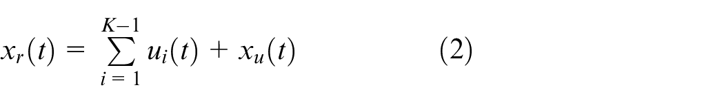
Keywords
Introduction
With the rapid development of science and technology, electric motors have found extensive applications in modern industry and daily life.1–3 Of all the failures, the majority of rotating machinery failures are caused by bearing failures. 4 Bearings are vital to the normal operation of motors, bearing loads, reducing friction, protecting critical components, and ensuring smooth operation and efficient performance. 5 Rolling bearings use rolling elements to reduce friction and have a lower friction factor, which not only reduces energy loss, but also reduces the heat generated due to friction, contributing to the efficient operation and longer life of the drive motor. Moreover, rolling bearings can absorb and reduce the loads and impacts caused by road shocks and vibrations, play a cushioning role, and protect the motor and other key components from excessive stress and damage.6–8 Therefore, accurately diagnosing motor bearing faults is very significant. Through the efforts of researchers and scholars at home and abroad, rolling bearing fault diagnosis has been widely studied from the traditional manual extraction of data and analysis of the cause of the fault to the current autonomous diagnosis relying on deep learning in the field of artificial intelligence.
Common signal decomposition methods include Fourier transform, Wavelet transform, and Empirical Mode Decomposition (EMD), among which EMD has been widely used. Qi et al.
9
developed a bearing fault diagnosis technique that integrates empirical mode decomposition, deep learning, and knowledge graphs to enhance multi-dimensional feature extraction and provide comprehensive fault information, achieving high accuracy even under varying loads and noisy conditions. However, challenges such as, mode overlap and pseudo-modes at signal boundaries persist with EMD. In 2014, Dragomiretskiy and Zosso
10
proposed Variational Mode Decomposition (VMD), which improves upon EMD by using a non-recursive decomposition model and ensuring stable results through the construction of a variational problem. Zhou et al.
11
advanced rolling bearing fault diagnosis by incorporating the Whale Gray Wolf optimization algorithm, variational mode decomposition, and support vector machine (SVM) to effectively diagnose faults in nonlinear and nonstationary vibration signals. Zhen et al.
12
developed a fault diagnosis method that combined VMD with cyclostationarity demodulation to extract fault characteristics from noisy bearing signals. VMD also has some limitations, such as reliance on the number of mode components
Conventional diagnostic methods are usually based on time domain, frequency domain and time-frequency domain.19–21 Song et al. 22 introduced a visual diagnosis method leveraging incrementally accumulated holographic symmetrical dot pattern characteristic fusion to enhance signal differentiation. Samal et al. 23 developed a bearing fault diagnosis approach using artificial neural networks combined with vibration analysis for higher classification accuracy. However, traditional fault diagnosis techniques depend on the experience and expertise of technicians to identify faults, which have significantly limited the development of rolling bearing fault diagnosis. (1) Since the feature extraction relies heavily on the knowledge and judgment of engineers, this may cause errors where minor fault indicators will be mistakenly discarded or obscured by noise.24,25 (2) The extracted features are mainly used to solve specific fault problems, making them less generalizable. (3) Under actual working conditions, bearings often operate under variable loads and speeds, which leads to the fluctuating pulse intervals and causes challenges in feature extraction, and the signal noise contamination in the vibration signals collected by the system.26,27 Thus, the traditional manual fault diagnosis cannot solve the problem of fault diagnosis of the bearings under these conditions.
Deep learning has powerful nonlinear modeling and automatic feature extraction capabilities, such as AutoEncoders, Deep Belief Networks, Convolutional Neural Networks, and Recurrent Neural Networks. Rajabioun et al. 28 developed a deep learning framework that combined multi-sensory input from vibration and magnetic flux signals to effectively diagnose distributed bearing faults. Ding et al. 29 introduced a channel attention siamese network with metric learning for intelligent bearing fault diagnosis, achieving high accuracy even with very small sample sizes and maintaining the reliability under noise and signal distortion. Niu et al. 30 presented a deep residual CNN that enhanced discriminate feature learning and integrated domain knowledge, improving diagnostic accuracy and training efficiency for multitask bearing fault diagnosis. Jiaocheng et al. 31 employed a Bayesian optimization-deep convolution gate recurring unit method to automatically adjust hyperparameters, enabling precise bearing fault identification and overcoming traditional experience-based adjustment limitations. However, the aforementioned studies overlook the spatiotemporal correlations in vibration signals. Although these studies achieve relatively good fault diagnosis performance, there is still room for improvement.
Considering the shortcomings of the aforementioned methods, several recently emerging approaches have effectively addressed some of these issues. Liu et al. 32 proposed a Siamese CNN-BiLSTM model designed to fully extract the multidimensional and temporal features of rolling bearing vibration signals to better learn the advanced features of different fault types of signals. Wang et al. 33 introduced a WOA-VMD and the GAT to overcome the effect of noise on the signal. WOA-VMD is used to decompose the original signal, then the KNN method is used to construct the graph structure data. The attention mechanism is used to construct the fault diagnosis model of the GAT rolling bearing in order to classify the signal. Feng et al. 34 developed a new MHA mechanism that integrates positional information into the weight matrix, thereby enabling it to extract more effective data features compared to the traditional MHA method. Additionally, the proposed method is developed for fault diagnosis scenarios that involve missing information.
In summary, accurate bearing fault diagnosis is fraught with many challenges, such as the integrity of the raw input signals and the feature extraction capabilities of the model, both of which can directly impact the fault classification results. Although numerous studies have been conducted to address these challenges, there are still some limitations that prevent sufficient noise reduction in the signals and hinder the model’s ability to fully extract features. Inspired by the limitations of the aforementioned existing methods, a WOA-SVMD and multi-scale CNN-Transformer-based fault diagnosis method is proposed for signal denoising and fault classification to address the issues mentioned above. The innovation of our proposed method lies in the use of SVMD for signal decomposition instead of traditional VMD. The advantage of the SVMD method is that it requires the adjustment of only one parameter, the penalty factor
Taking the above into account, a WOA-SVMD and multi-scale CNN-Transformer method is proposed for denoising and fault classification of bearing vibration signals. Firstly, the vibration signals obtained from the sensors are decomposed by SVMD, the parameters of which are optimized by the WOA algorithm with minimal envelope entropy. The generated IMFs are then filtered by the Pearson correlation coefficient method and reconstructed into new signals. Secondly, multi-scale CNN is used to extract local features from the processed data, and the Transformer is applied to further explore the global features. Finally, the output is fed into the softmax function for fault classification.
The contributions of our work can be summarized as follows:
(1) A combined WOA-SVMD and multi-scale CNN-Transformer fault diagnosis model is proposed to address the problem of noise interference in the real operating environments and elevate the fault diagnosis accuracy.
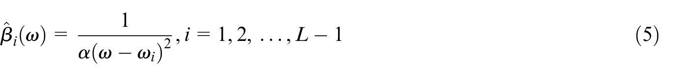
(2) To remove the noise variables in vibration signals, a combined WOA-SVMD and correlation coefficient method is proposed. This method optimizes the penalty factor parameter of SVMD to achieve the best decomposition results, while the correlation coefficient method is employed to filter out noise components with low correlation.
(3) To achieve adequate feature extraction, a combined multi-scale CNN-Transformer model is proposed. Multi-scale CNN extracts multiple localized features at various high-energy specific frequencies by using different sizes of convolution kernels, constructing rich feature representations, while transformer capture global features through its self-attention mechanism.
The remainder is arranged as follows: Section 2 proposes the architecture of the WOA- SVMD and multi-scale CNN-Transformer, covering WOA optimization, signal decomposition, filtering, multi-scale convolution, multi-head attention, and fault classification. Section 3 shows the experimental results. The conclusion is provided in Section 4.
The proposed fault diagnosis method
The overall framework of the proposed method is illustrated in Figure 1. The model is composed of data processing, multi-scale CNN and Transformer Encoder for feature extraction and fault type classification. In this study, vibration signal data was collected by placing an accelerometer on the drive end of the motor housing. The fault diagnosis process involves three main steps.
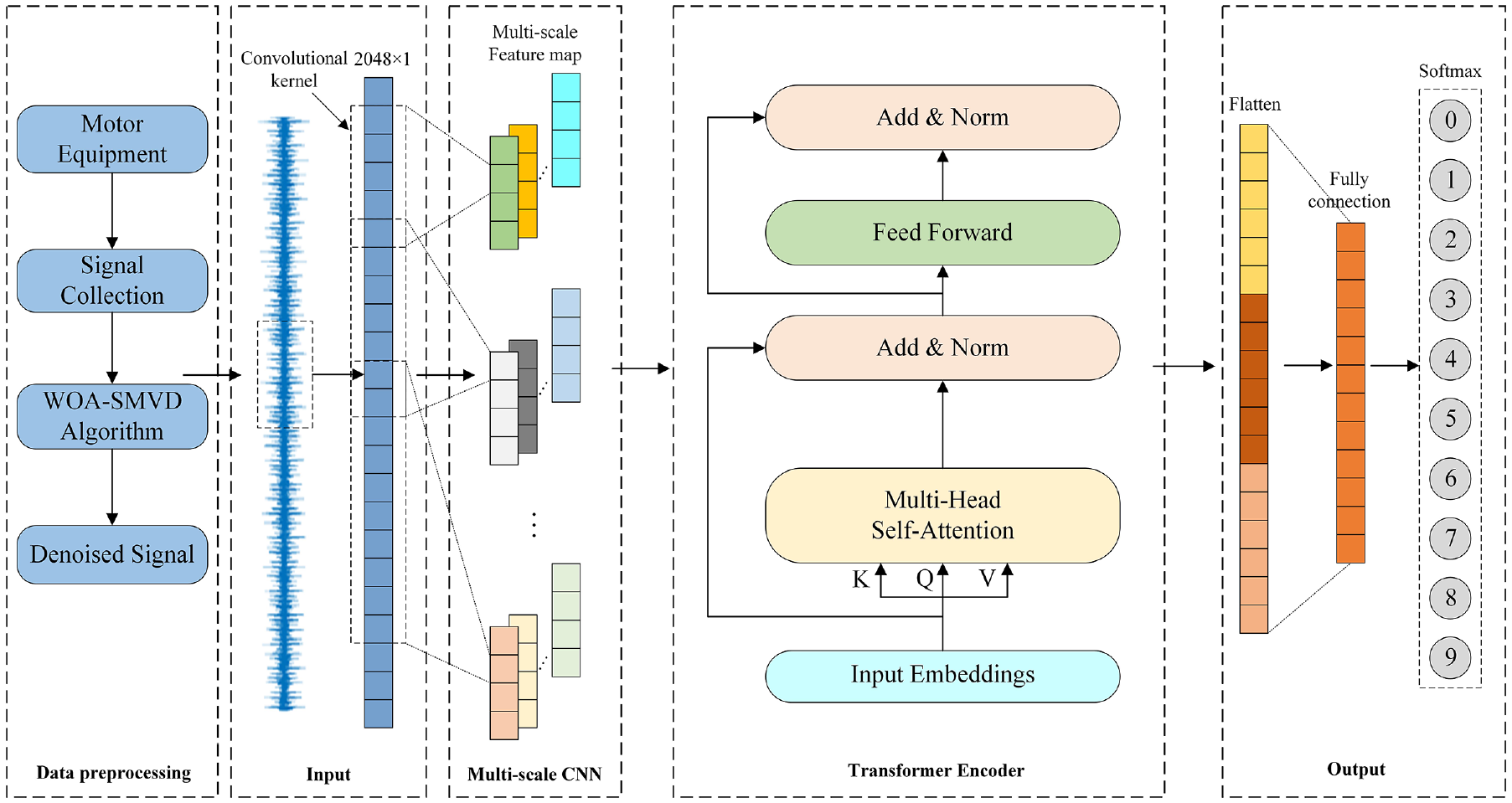
Framework of proposed WOA-SVMD and multi-scale CNN-Transformer model.
Firstly, a data preprocessing model is established. The vibration signal collected by the accelerometer is susceptible to ambient noise. Common signal decomposition methods require preset parameter values. For instance, the VMD method necessitates a predetermined mode components
Secondly, a combined multi-scale CNN and Transformer feature extraction model is developed to leverage the strengths of both approaches and complement each other. CNN excels at extracting local features by utilizing convolutional kernels that slide across different regions of the input, efficiently capturing localized patterns in the data. On the other hand, the Transformer is known for its ability to extract spatial features through its unique self-attention mechanism, which enables it to dynamically adjust its focus on various parts of the input. This allows the Transformer to flexibly and effectively capture global spatial features, avoiding the limitations of relying solely on local information. By integrating these two methods, the model is able to fully capture both local and spatial features, leading to improved fault diagnosis accuracy.
Finally, the extracted features are flattened, and the fault categories are predicted using a fully connected layer followed by a softmax function. The predicted categories are then compared to the actual fault categories to calculate the loss value, which is used to continuously optimize the model’s classification performance.
WOA-SVMD model establishment
Signal denoising is an critical part of data preprocessing. A lot of useless noise in the input data will not only lead to poor qualities of learned features, but also lower the convergence speed of model training, or even fail to converge. 35
SVMD optimized by WOA
One of the main challenges with VMD is the need to accurately preset the number of modes
Assuming the input signal

where
The SVMD method for the
where
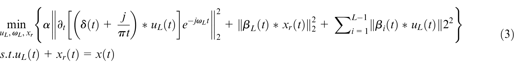
To transform the constrained minimization problem described in equation (3) into an unconstrained optimization problem, the quadratic penalty term and Lagrangian multiplier
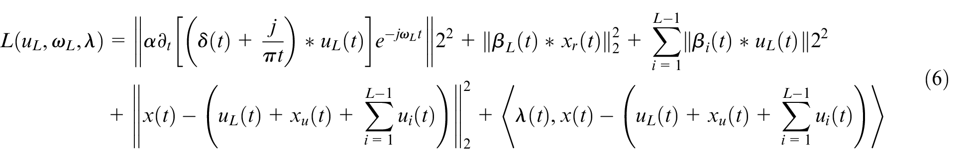
According to Parseval’s theorem, equation (6) can be transformed into its frequency domain form and rewritten as:
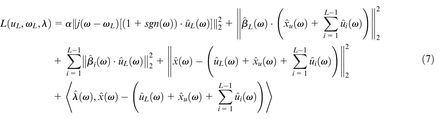
As in the VMD and VME methods, the alternate direction method of multipliers(ADMM) algorithm is also employed to iteratively solve the above minimization problem. The detailed solution process can be found in Nazari and Sakhaei.
16
The final iteratively updating equations of
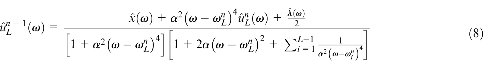
where
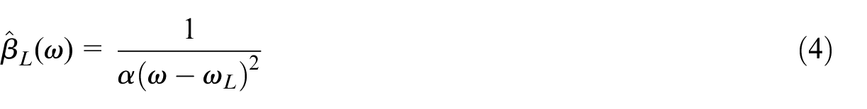
Among the above iterative updates, it’s clear that an appropriate value for the penalty parameter

where


where
where
The simulation of the humpback whale’s unique hunting technique involves a spiral motion to update its position and a narrowing ring mechanism, commonly referred to as the bubble net strategy. The probability of successfully capturing prey with these two methods is assumed to be 50%. When the probability

where
In addition to the bubble net strategy mentioned above, the whale also hunts based on its position, again by adjusting vector

where
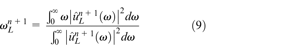
Subsequently, select the minimum value of envelope entropy as the fitness function. The envelope entropy reflects the sparsity of the original signal. A higher envelope entropy value indicates more noise and less meaningful information in the IMF, while a lower value suggests less noise and more effective information. The envelope spectrum of the signal
where
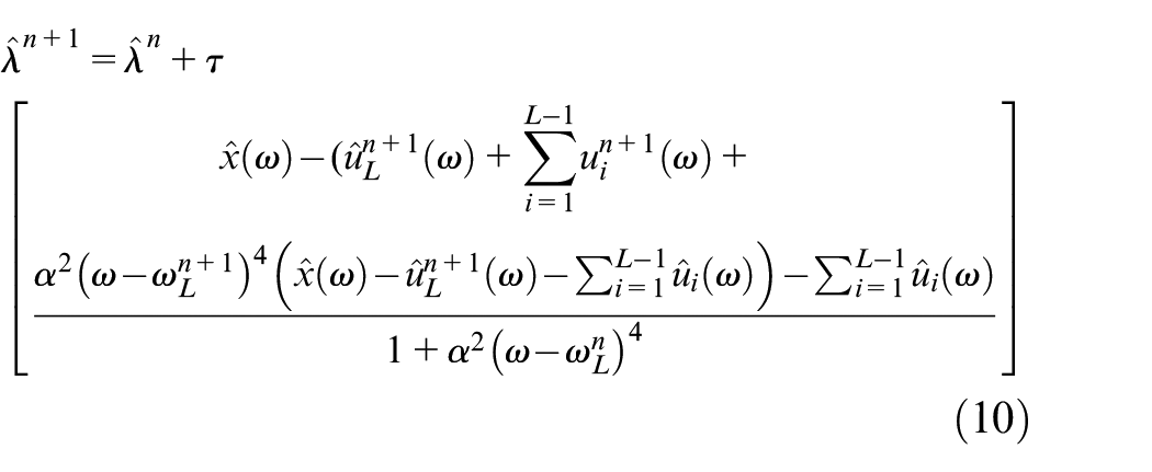
After obtaining the optimal whale position using WOA, it is used in updating the parameters for
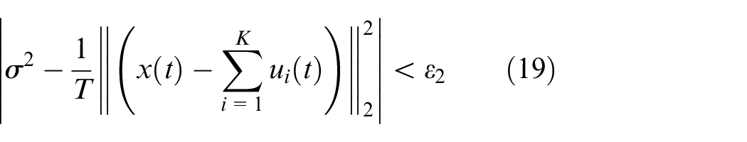
The stop criteria for updating parameters
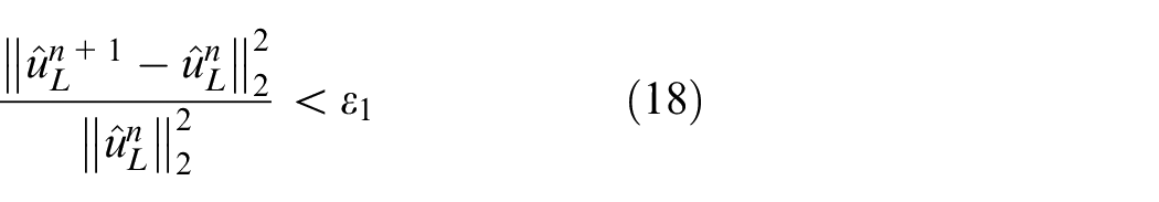
The termination criteria of SVMD is expressed as:
where
Process of WOA optimized SVMD
The flowchart of optimizing the SVMD parameters using WOA is shown in Figure 2. The specific steps are as follows:
Step 1: The ranges of the SVMD parameter to be optimized are set and the WOA model is initialized, including the population size, the maximum iteration number. Here, penalty factor
Step 2: Decompose the input signal by using SVMD and obtain each IMF function. Calculate the envelope entropy of each IMF by using equation (17). The envelope entropy was used as a fitness function to find the optimal whale location and retain it;
Step 3: Start the iteration. A random number
Step 4: Determine the value of
Step 5: Calculate each whale’s fitness and compare it to the previously stored optimal position. If the new solution is better, replace the previous one with the new optimal solution.
Step 6: Determine whether the iteration is terminated. If
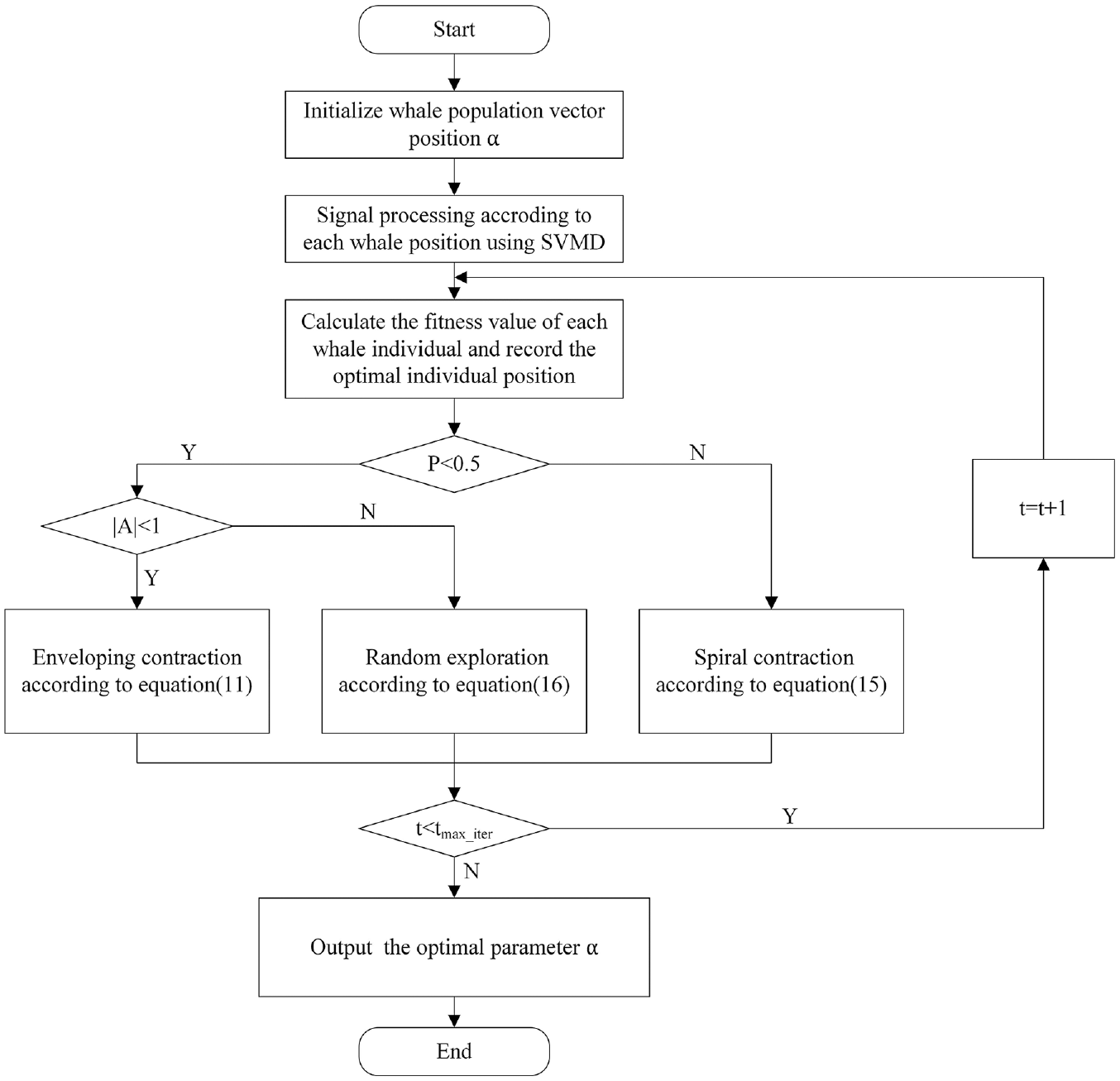
The flowchart of WOA optimizing SVMD.
Signal denoising process
After SVMD decomposition, the signal is broken down into a series of IMFs, each corresponding to a distinct frequency component of the original signal. These IMFs are well-localized in the time domain and exhibit concentrated energy distribution in the frequency domain. Next, Pearson correlation coefficients are calculated between each IMF and the original signal. IMFs with correlation coefficients higher than 0.2 are selected because they closely resemble the original signal and retain more meaningful information. In contrast, IMFs with low correlation coefficients are likely to contain more noise or irrelevant components.
The correlation coefficient is a statistic used to describe the strength of the linear relationship between variables. In this paper, the Pearson correlation coefficient is used. The coefficient ranges from
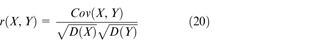
where
Then, the retained IMFs are reconstructed to obtain the denoised signal. The denoising effect is evaluated by Mean Squared Error (MSE) and Signal-to-Noise ratio (SNR). The expressions for these metrics are as follows:
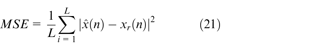
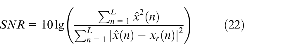
where
Multi-scale CNN-Transformer model for fault classification
Multi-scale CNN-Transformer method
For time-series vibration signals, 1D-CNN performs local feature extraction via convolution kernels, which has the advantages of relatively simple structure, lower computational complexity, and reduced risk of overfitting. Small kernel sizes can capture the high-frequency features of the vibration signal, while large kernel sizes can capture the low-frequency features of the vibration signal. For example, when the original signal has a sampling rate of 48 kHz, if a 1D-CNN with a convolutional kernel size of 120 is employed, the kernel covers a time window of roughly 2.5 ms, which primarily captures frequency features at or below 400 Hz. On the other hand, if the convolutional kernel size is reduced to 6, the kernel covers a much shorter time window of about 0.125 ms, enabling the extraction of high-frequency features up to 8 kHz.
CNNs are primarily composed of convolutional layers, batch normalization layers, pooling layers, activation layers, and so on. They learn and extract features from input data through local connections and weight sharing, using classifiers for supervised classification predictions. 37
The one-dimensional standard convolution operation is given below:
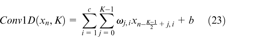
where
Multi-scale Convolution (MSC) makes use of convolution kernels of different sizes to extract features as shown below:
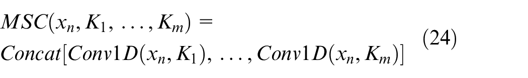
where
The weights
where
As can be seen from Figure 3, the frequency of the bearing vibration signal is mainly concentrated in 0–5000 Hz and 8400 Hz, so we used 1D-CNN with different sizes of convolutional kernels to accurately capture different frequencies. Eventually, convolutional kernels of eight different sizes were chosen: 6, 15, 18, 36, 48, 72, 96, 144.
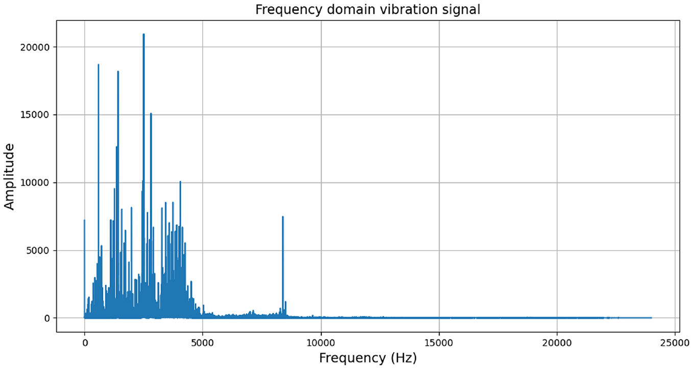
The frequency domain vibration signal of 0.18 mm inner-race fault.
After the convolution operation comes pooling, and the pooling process is represented as follows:

where
Subsequently, the activation function is applied to introduce nonlinearity, thereby enhancing the model’s representation capability. ReLU is one of the most commonly used activation functions in CNNs. It effectively mitigates the vanishing gradient problem and speeds up the convergence process. The ReLU function is mathematically defined as follows:
where
Finally, the feature maps generated by each convolution kernel are concatenated to create a multi-scale feature map. These feature maps will serve as the input to the Transformer for further global feature extraction.
In multi-scale CNN, each CNN consists of three convolutional layers, two max pooling layers, and a batch normalization layer. Additionally, ReLU activation function is used to preserve the non-linearity of MSCNN. Each pooling layer is applied to downsample the input. The specific hyperparameter settings are presented in Figure 4.
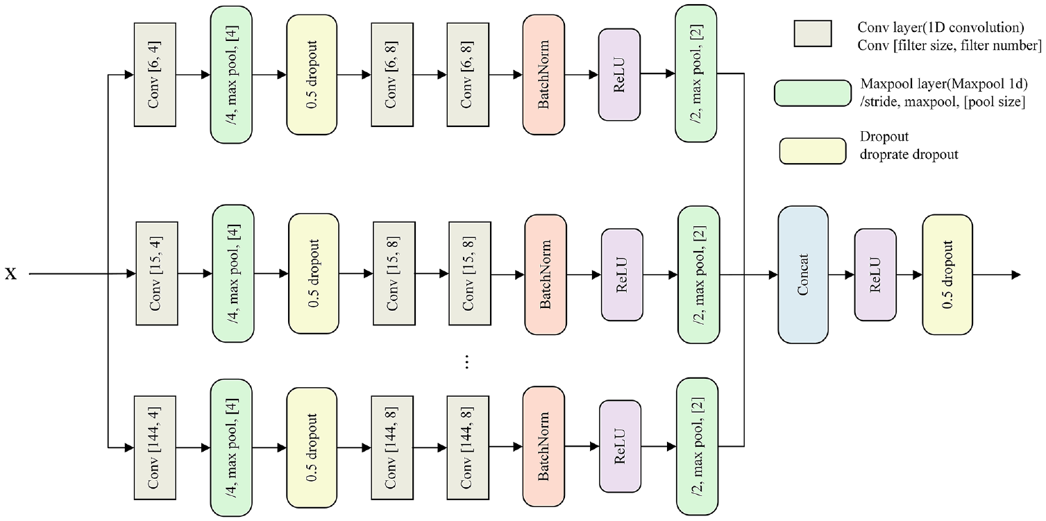
The specific architecture of multi-scale CNN.
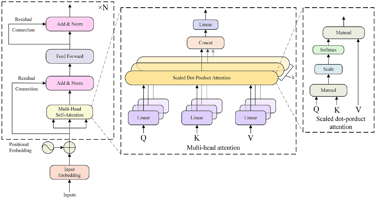
The Transformer network is a type of deep neural network based on the self-attention mechanism and is capable of extracting features in parallel and incorporating global feature modeling. A full Transformer network includes an encoder-decoder structure. However, the encoder for classification alone suffices as the core feature extractor, making the decoder superfluous. The architecture of transformer encoder is shown in Figure 5.
The architecture of transformer encoder.
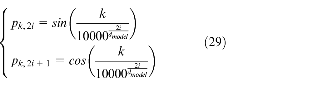
First of all, positional embedding is used to infuse positional information into these feature maps, enabling the model to recognize the relative or absolute position of each feature. This is especially important for time-series signals, where the order of data points is crucial. With Positional Embedding, the model can better capture the temporal relationships between features, thereby enhancing the understanding and representation of global features. The positional encoding is expressed as:
where
Then, two key modules are employed: the multi-head attention module and the feed-forward connection layer module. Multi-head attention is composed of
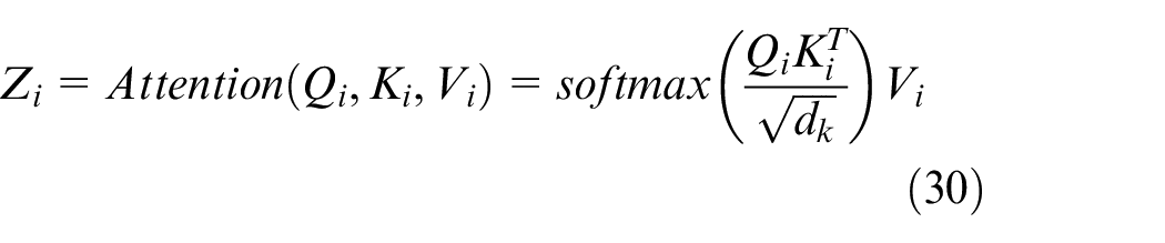
Finally, the individual attention heads are concatenated and linearly projected to generate the final attention output. The process can be summarized as follows:

where
where
The feed-forward connection layer module consists of two fully connected layers, with a ReLU activation function applied between them. Additionally, the Transformer model includes two normalization layers. Layer normalization plays a critical role in ensuring fast convergence and stable training of the Transformer. In summary, the architecture can be described as follows:


where
Classification
Classification is the final step in fault diagnosis, where the classifier outputs the predicted category. This predicted result is then compared with the actual category to assess its accuracy. Then, the model parameters are adjusted accordingly. Through continuous training and fine-tuning, the model is gradually optimized. Ultimately, we obtain the desired model, which can be used for the final testing phase.
Firstly, the final output of the Transformer is flattened using the Flatten function. Once flattened, the data is passed through the fully connected layer for further processing, ultimately generating the final classification results.
Then, the cross-entropy loss function is used to calculate the loss between the predicted category and the true category. Subsequently, backpropagation and optimization are performed using Adam optimizer. After 100 rounds of training, the optimal model for fault diagnosis is obtained.
Finally, the test set data is fed into the model for fault classification, thus, the fault diagnosis process is completed.
Overall flowchart of the proposed method
The flowchart of the WOA-SVMD and multi-scale CNN-Transformer method is shown in Figure 6, which mainly includes the following steps:
Step 1: Collect vibration signals under different fault types.
Step 2: Use WOA to obtain optimal parameter
Step 3: Use the optimal
Step 4: Calculate the Pearson correlation coefficients between these IMFs and the original signal. Set the retention threshold at 0.2, filtering out IMFs with correlation coefficients below this value. Reconstruct the signal to remove noise.
Step 5: Input the denoised signal into the model to extract feature vectors.
Step 6: The fault diagnosis results are then output through the fully connected layer and Softmax classifier.
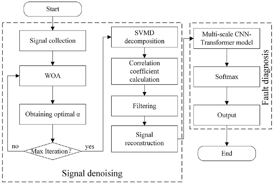
Overall flowchart of WOA-SVMD and multi-scale CNN-Transformer method.
Experimental verification
Validation based on CWRU bearing dataset
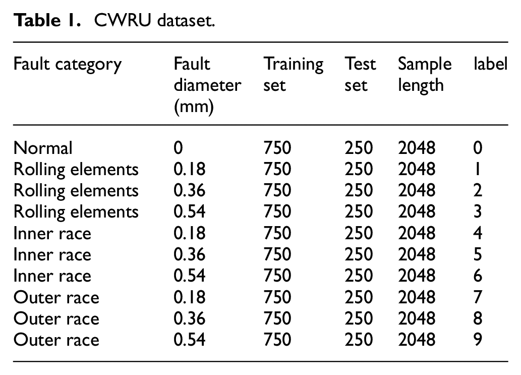
The SKF-6205 drive-end bearing fault data, sourced from the open-access bearing fault dataset by Case Western Reserve University (CWRU), was utilized as the experimental data in this study, as shown in Figure 7. 38 The raw data was collected from accelerometers mounted on the drive end, fan end, and base of the motor housing. For this study, the vibration data from the drive end was selected as the primary vibration signal. The dataset includes four health conditions: normal, inner race fault, outer race fault, and rolling element fault. Each fault type is available in three defect sizes: 0.18, 0.36, and 0.54 mm, resulting in a total of 10 categories of fault data. The vibration signals were recorded under engine loads and motor speeds of 0 hp/1797 rpm, 1 hp/1772 rpm, 2 hp/1750 rpm, and 3 hp/1730 rpm, with a sampling frequency of 48 kHz. In this study, the data corresponding to 3 hp and 1730 rpm were used. Further details are provided in Table 1.
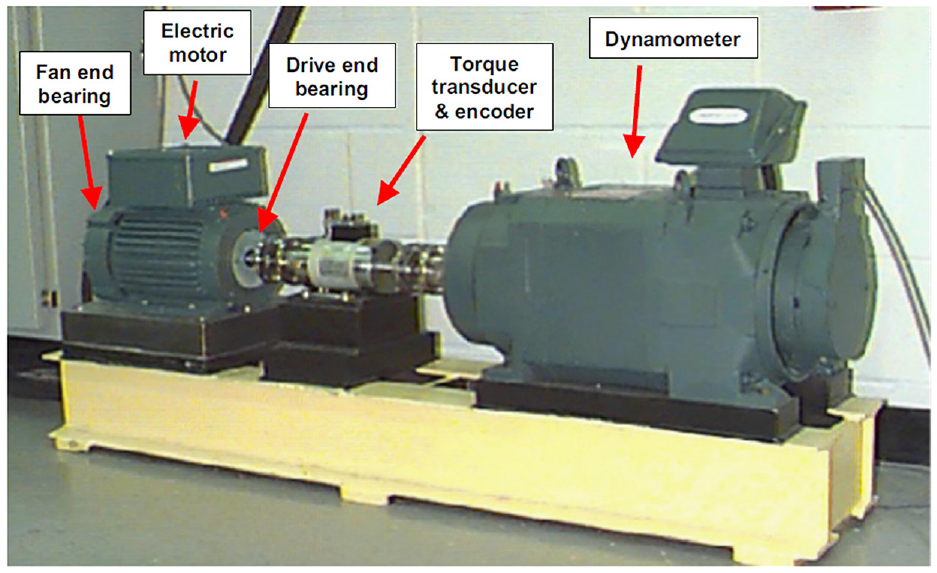
Testbed for the CWRU dataset.
CWRU dataset.
To avoid overfitting due to insufficient data, we employed a sliding window overlap sampling method for data augmentation, as illustrated in equation (36). In this equation,
The dataset is divided into training and test sets in a 75% to 25% ratio, respectively. Each state includes 750 samples in the training set and 250 samples in the test set, resulting in a total of 10,000 samples. The cross-entropy loss function is employed, with the Adam algorithm as the optimization method. All programs run on a computer with the following configuration: Intel i3 12100, NVIDIA RTX 3080.
WOA-SVMD denoising results
This experiment used a dataset with rolling element faults by selecting the bearing early fault signal of 1024 points starting from time t = 0.
Firstly, 5 dB noise is added to the original signal. A higher dB value indicates less noise, while a lower dB value indicates more noise. As shown in Figure 8, the signal change is quite noticeable after adding the noise.
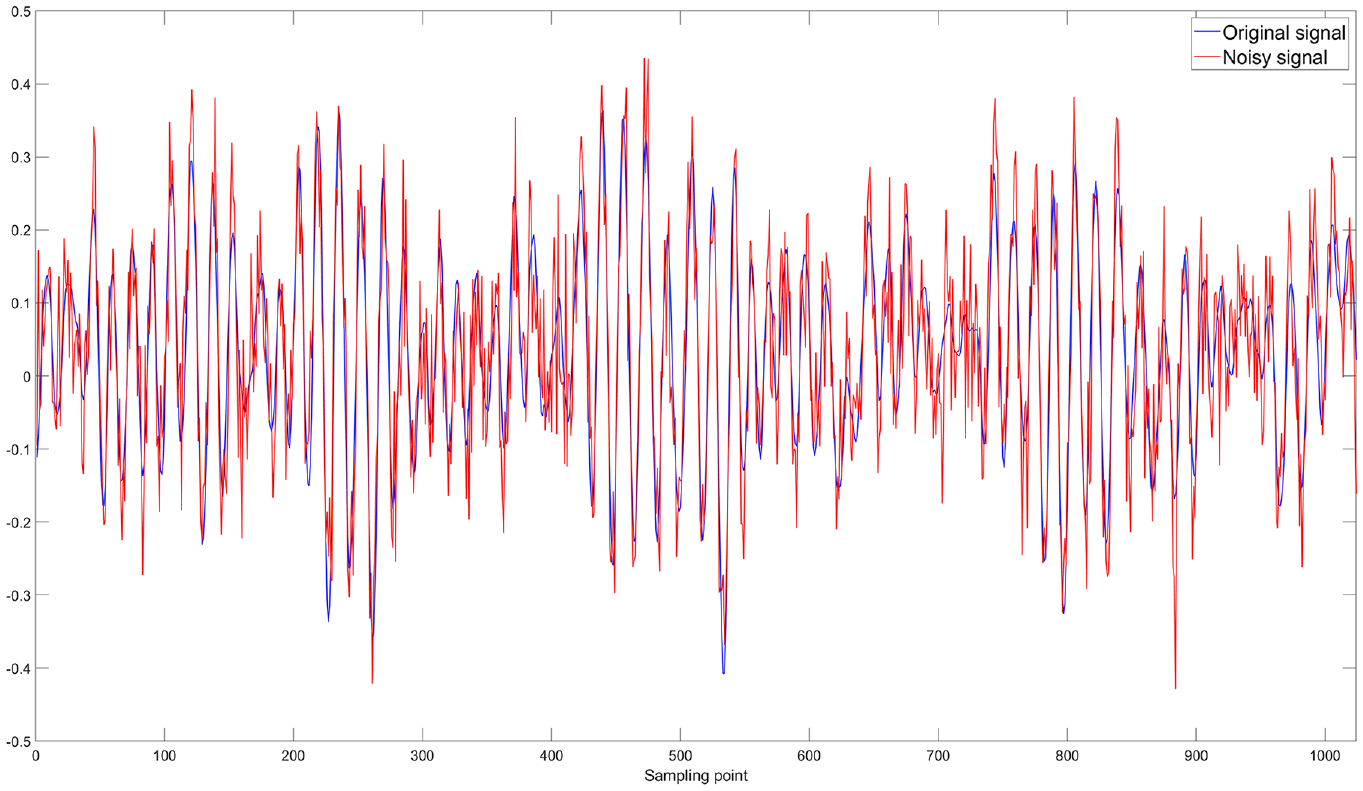
Comparison between the original signal and the noise-added 5 dB signal.
Then, the optimization iteration curve of WOA is illustrated in Figure 9, which shows that the algorithm converges after 5 iterations, resulting in a minimum envelope entropy of 6.76735 and an optimal penalty factor value of 2445.7462.
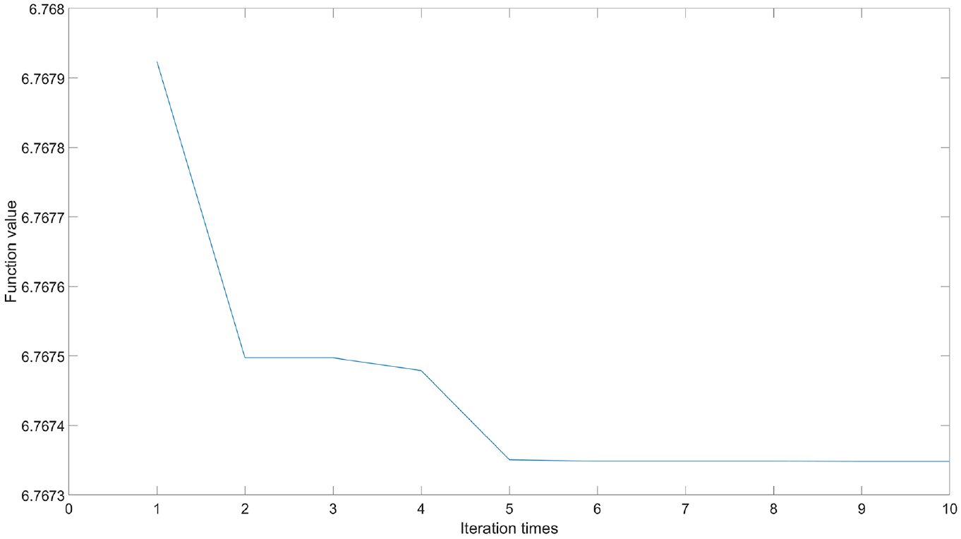
Optimization iterative curve of WOA.
Next, the optimal penalty factor parameter α is applied in the SVMD algorithm for signal decomposition, resulting in a series of IMFs, as shown in Figure 10. Typically, low-frequency IMFs represent the trends or slow variations in the signal, while high-frequency IMFs contain detailed information about noise or rapid oscillations. To better visualize the IMFs, they are displayed in a 3-dimensional space, as illustrated in Figure 11, allowing a clearer view of each IMF component. Subsequently, the amplitude spectrum, power spectrum, and frequency spectrum of each IMF are calculated to further analyze their frequency characteristics, as shown in Figures 12–14, respectively. The amplitude spectrum shows the intensity of each frequency component within the IMF, aiding in the identification of dominant frequencies. The power spectrum reveals how the IMF’s power is distributed across frequency components, indicating the frequency range where energy is concentrated. The frequency spectrum displays the distribution of various frequency components within the IMF, providing insight into the signal’s frequency structure. A Hilbert transform is also performed on each IMF to compute its instantaneous amplitude and instantaneous phase, and subsequently, the instantaneous frequency is calculated, which reflects the variation in the IMF’s frequency over time. The instantaneous amplitudes and instantaneous frequencies of all IMFs are then synthesized along the time axis to generate a three-dimensional Hilbert spectrum. This spectrum illustrates the energy distribution of the signal in the time-frequency plane, revealing the strength of each frequency component at every moment in time. The results are presented in Figure 15.
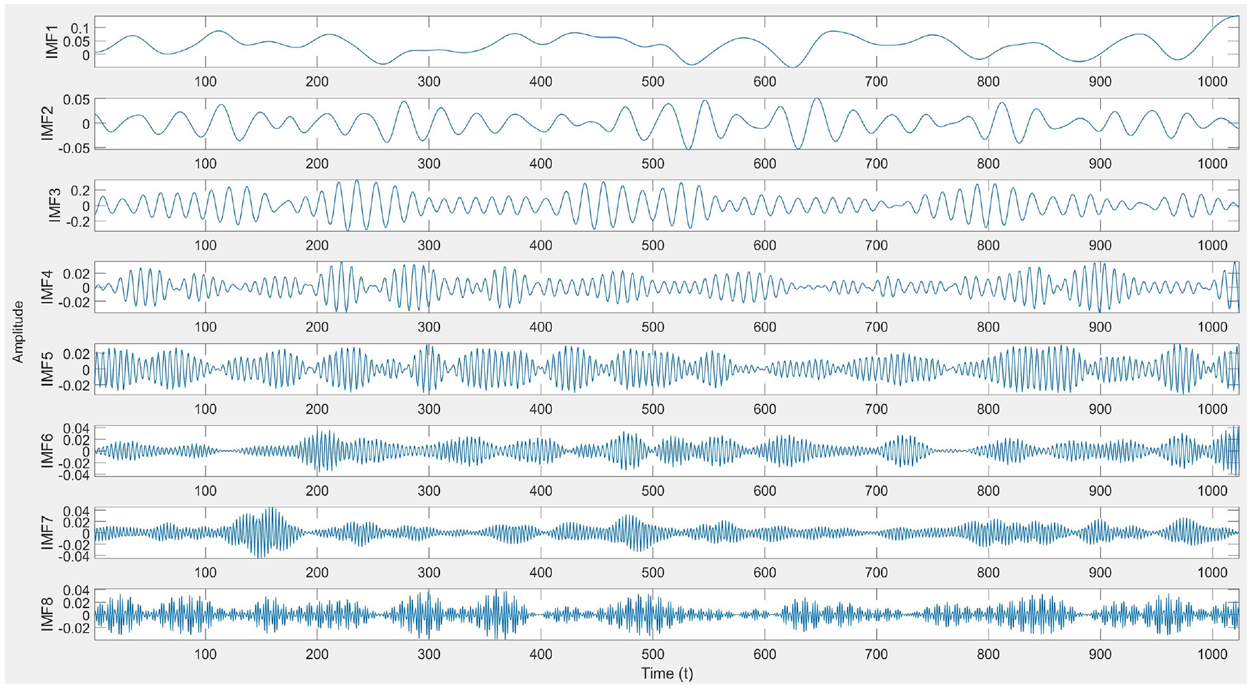
IMF components decomposed by SVMD.
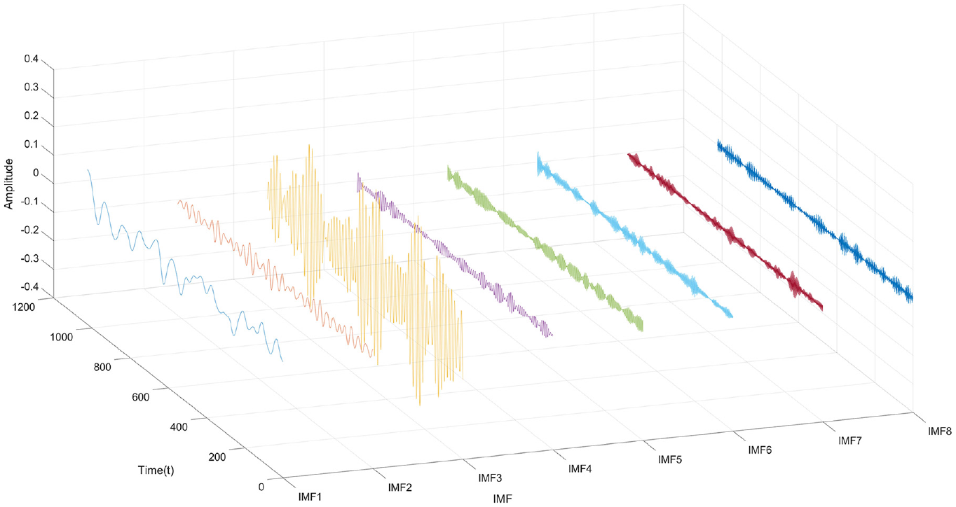
3D-IMF components decomposed by SVMD.
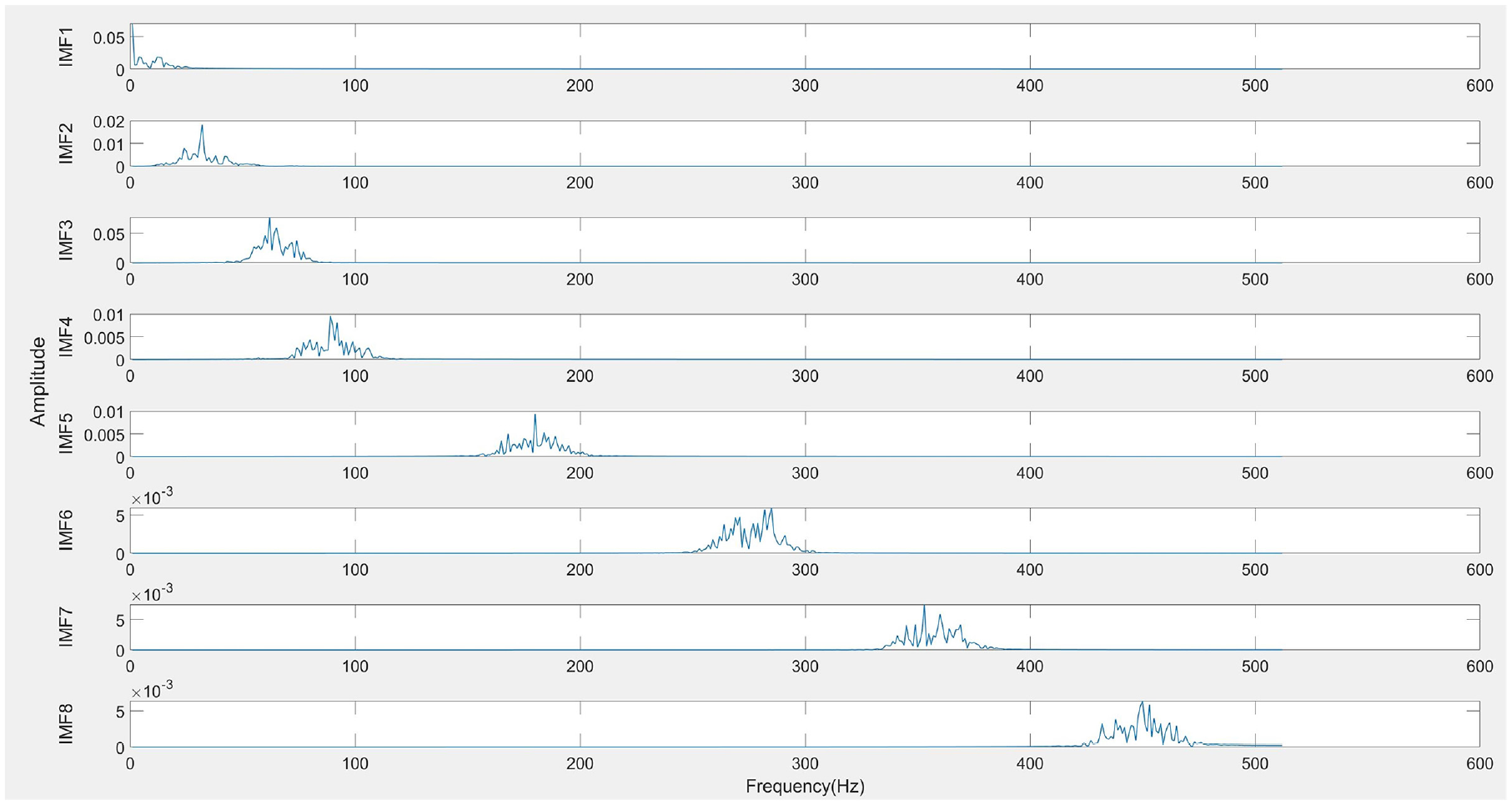
Amplitude spectrum of each IMF.
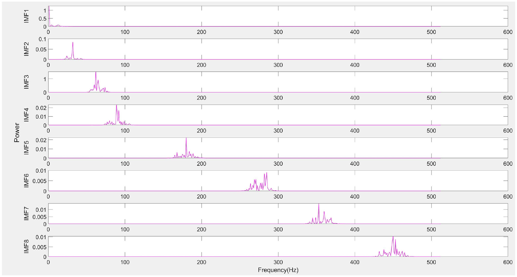
Power spectrum of each IMF.

Frequency spectrum of each IMF.
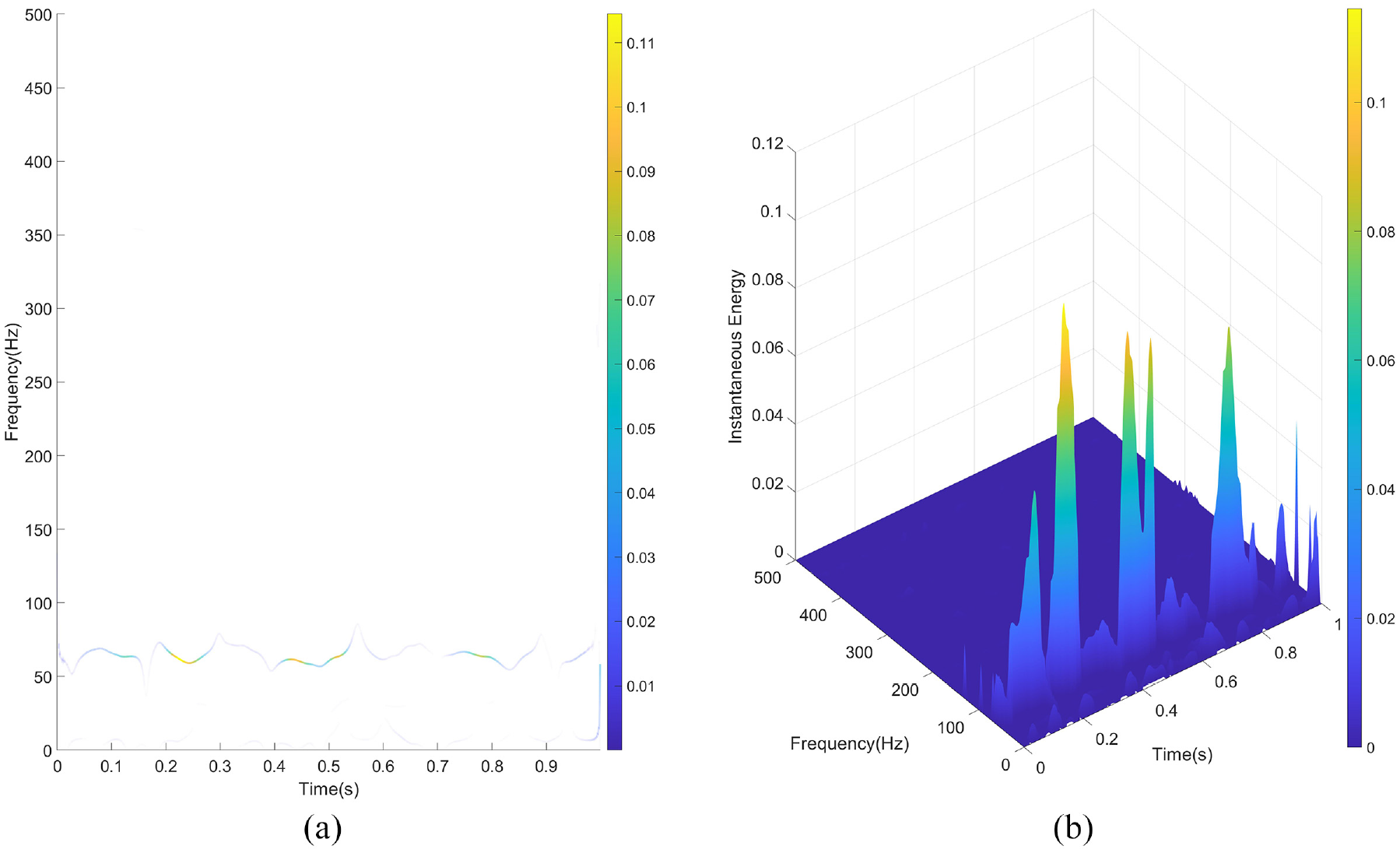
Hilbert spectrum of each IMF: (a) 2D-Hilbert spectrum and (b) 3D-Hilbert spectrum.
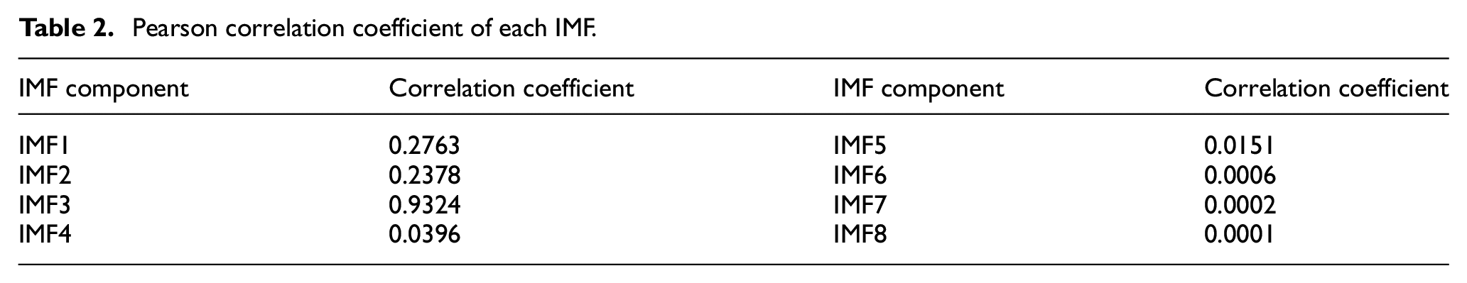
Finally, the Pearson correlation coefficients between each IMF and the original signal are calculated, with the results presented in Table 2. The IMFs with correlation coefficients greater than 0.2 are retained and used to reconstruct the signals for denoising. To verify the effectiveness of the proposed method, the denoised signals are compared with the original signals, and the comparison is shown in Figure 16. Two other signal decomposition methods, WOA-VMD and GWO-CEEMDAN, are also included for comparison. The denoising effect with different dB levels of noise added to the original signal is shown in Figure 17. It is important to note that the parameters optimized for VMD were the number of modes
Pearson correlation coefficient of each IMF.
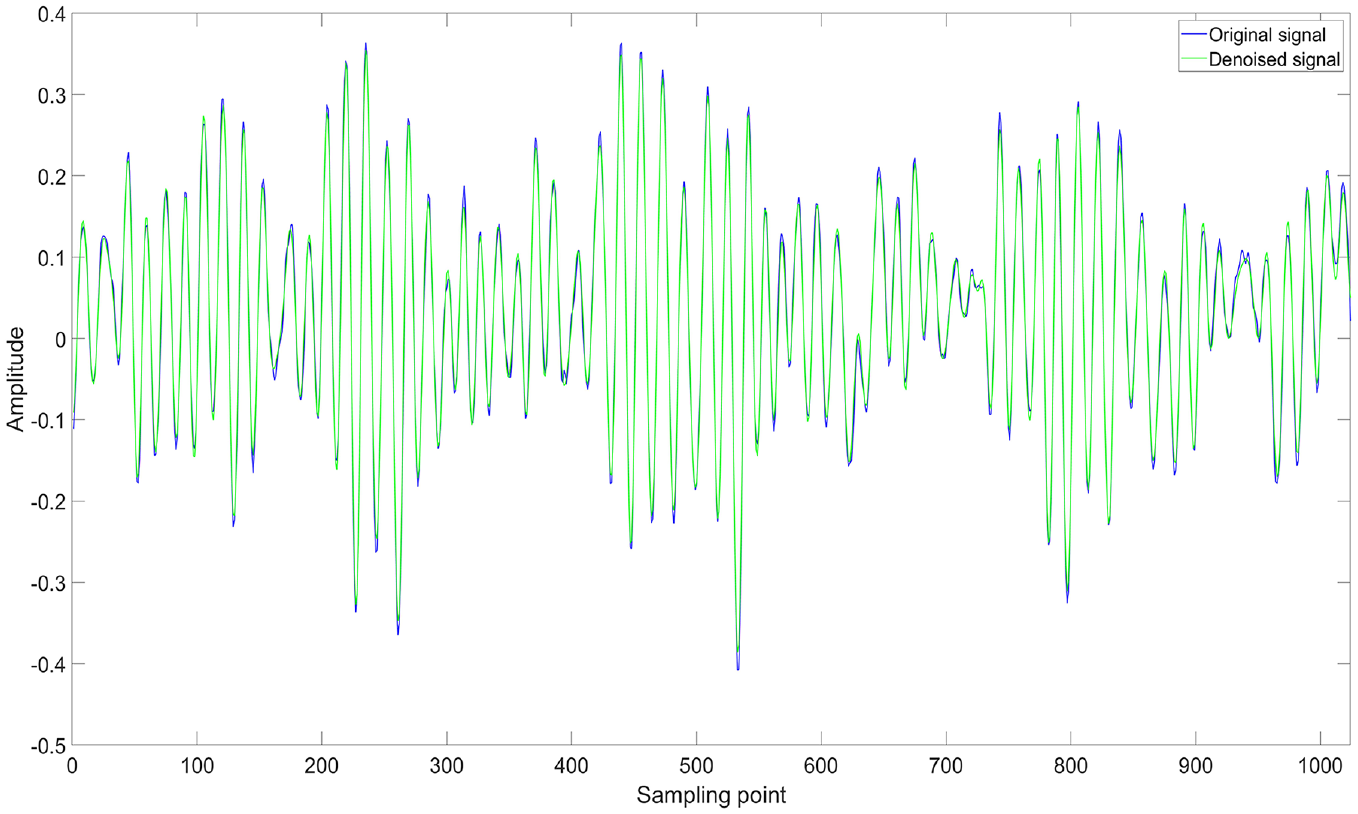
Comparison of denoised signal with original signal.
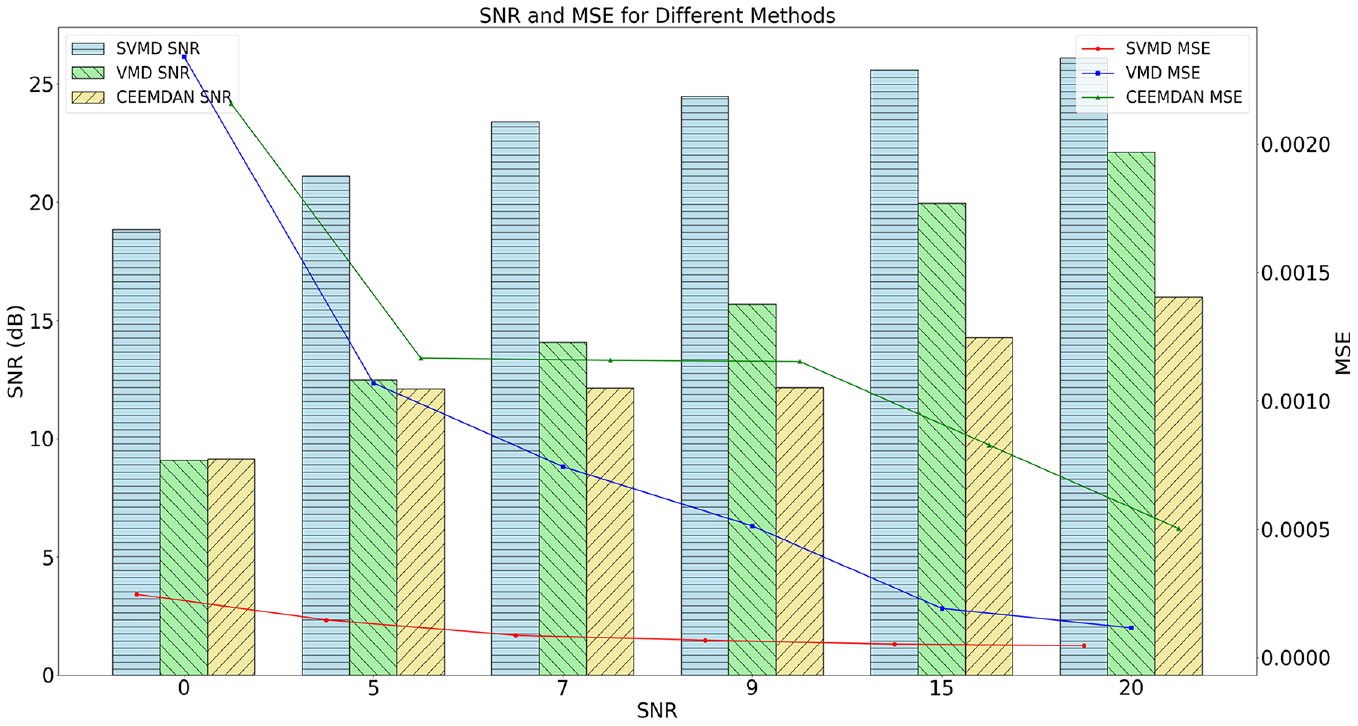
Comparison of denoising results of different methods.
Multi-scale CNN-Transformer classification result
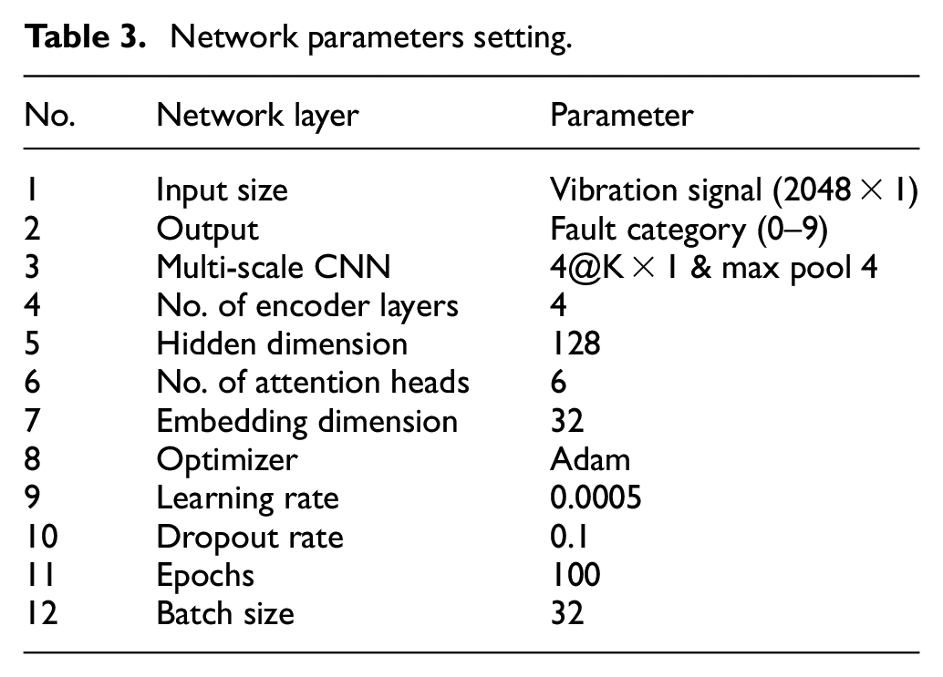
In this experiment, the model parameters were configured as follows: embedding dimension, hidden dimension, number of attention heads, number of encoder layers, and dropout rate. When the embedding and hidden dimensions are too small, the network becomes under-parameterized, resulting in degraded performance. Additionally, a lower number of attention heads can cause the model to overly focus on its own position, leading to overfitting. The final model parameters are detailed in Table 3. The parameter
Network parameters setting.
The loss values and accuracy curves during the training of the multi-scale CNN-Transformer model are displayed in Figure 18. Figure 19 presents the confusion matrix on the CWRU dataset. The confusion matrix illustrates the comparison between the models’ predictions and the actual labels across different categories. In this matrix, the horizontal axis represents the true categories, while the vertical axis represents the predicted categories. The diagonal line indicates the number of correct predictions, while the off-diagonal elements represent the number of incorrect predictions. To visualize the features extracted by the models, T-SNE visualization in Figure 20 displays the high-dimensional features from the final hidden layer reduced to a two-dimensional vector distribution. The effectiveness of the models’ feature extraction capabilities is demonstrated through the similarity and clustering of the data points in these plots. To further assess the effectiveness of the multi-scale CNN-Transformer model, five additional models were selected for comparative analysis.39–41
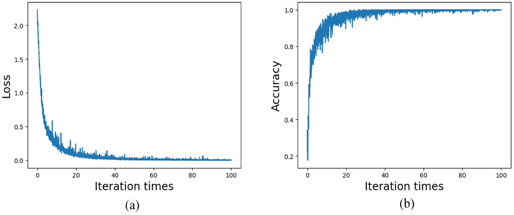
Loss values and accuracy curves of multi-scale CNN-Transformer model of the CWRU dataset: (a) loss curve and (b) accuracy curve.

Confusion matrix of multi-scale CNN-Transformer of the CWRU dataset.
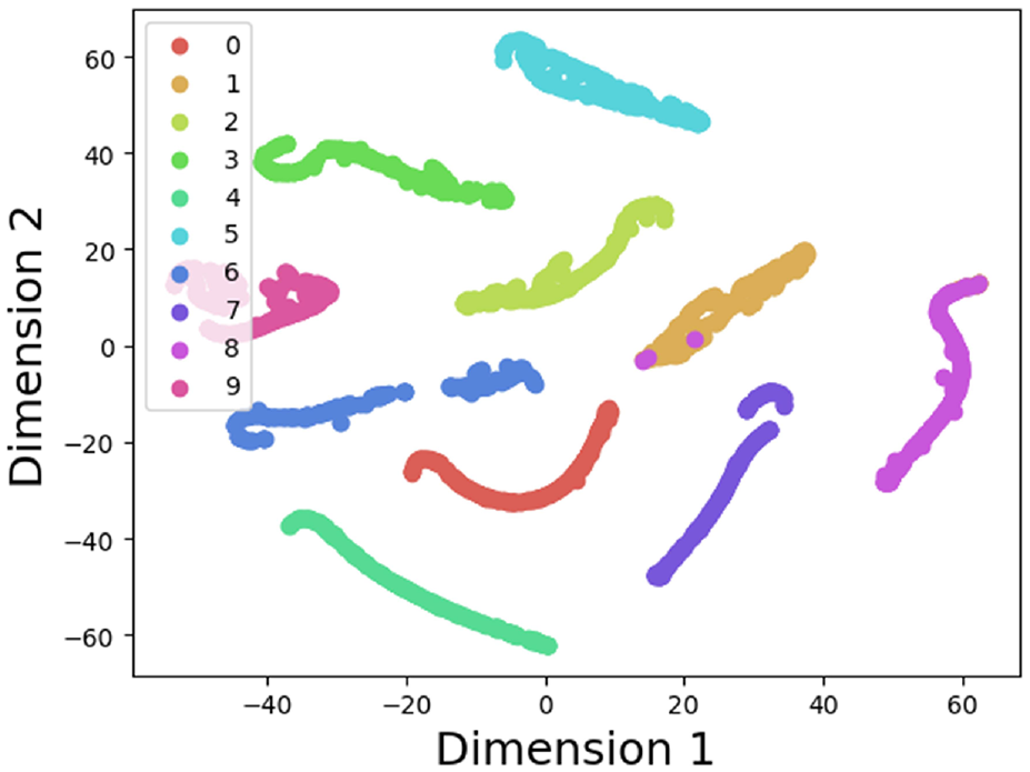
T-SNE visualization of the CWRU dataset.
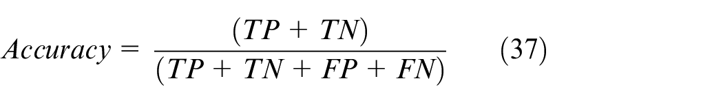
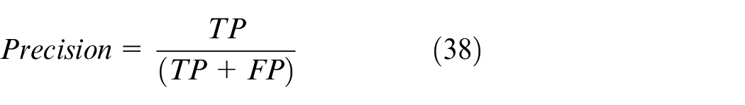
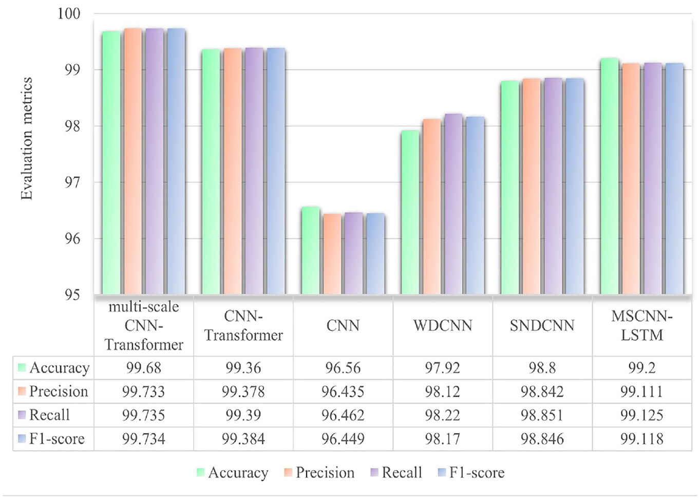
In the test dataset, the multi-scale CNN-Transformer network has a higher fault diagnosis accuracy of 99.24% than the other three networks. This proves the superiority of combining Transformer network and multi-scale CNN for fault diagnosis. Additional details on the model’s performance differences can be seen in the confusion matrix in Figure 21. To further evaluate the performance of the proposed method, a detailed comparison was conducted using four metrics: accuracy, precision, recall, and F1 score. True Positive (TP) refers to instances where the classifier correctly identifies the positive class. True Negative (TN) occurs when the classifier correctly identifies the negative class. False Positive (FP) represents cases where the classifier incorrectly labels a negative instance as positive, while False Negative (FN) occurs when a positive instance is incorrectly classified as negative. Accuracy measures the proportion of correct predictions out of the total predictions, reflecting the model’s overall correctness. The formula is provided in equation (37). Precision assesses how many of the predicted positive instances were actually correct, focusing on the accuracy of positive predictions, with the formula shown in equation (38). Recall evaluates how well the model identifies actual positive instances, emphasizing its ability to detect all positive cases, as outlined in equation (39). The F1 score, the harmonic mean of precision and recall, combines these metrics into a single measure. It is particularly valuable when class distribution is imbalanced or when balancing precision and recall is crucial. A high F1 score indicates minimized false positives and false negatives, as detailed in equation (40). A detailed comparison of the model’s performance using these four metrics is shown in Figure 22.
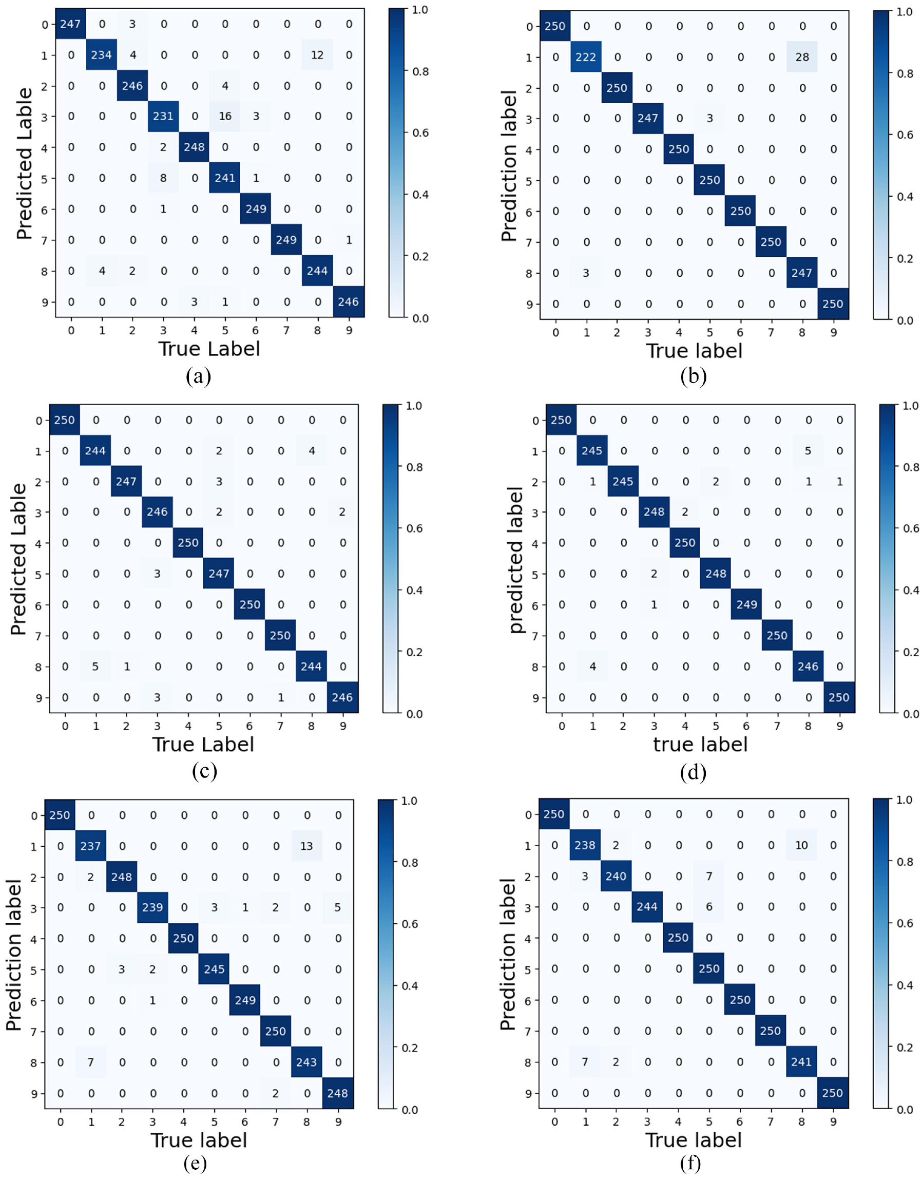
Confusion matrix of different model of the CWRU dataset: (a) CNN, (b) WDCNN, (c) CNN-Transformer, (d) multi-scale CNN-Transformer, (e) SNDCNN, and (f) MSCNN-LSTM.
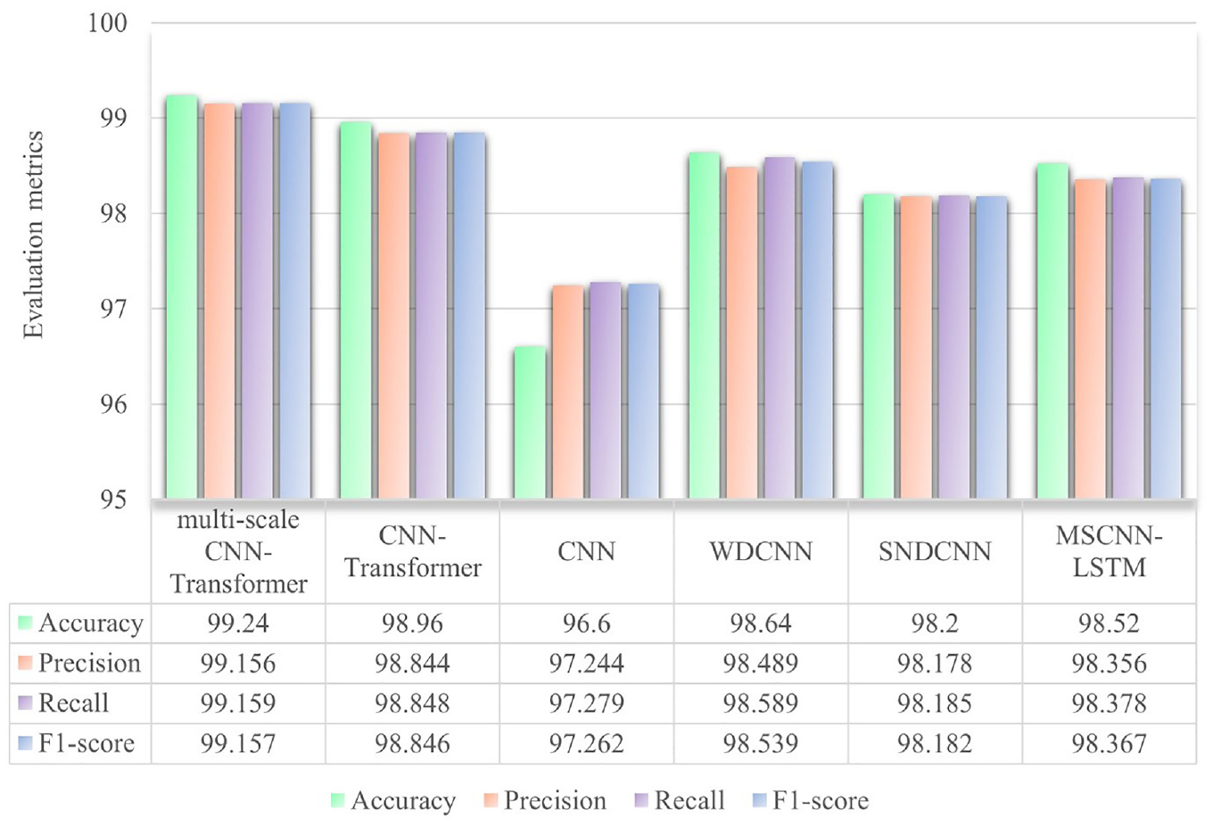
Comparison of different methods using four performance evaluation metrics of the CWRU dataset.
Validation based on PU bearing dataset
The PU dataset is provided by the Paderborn University Bearing Data Center and is widely used in bearing fault diagnosis research. 42 The test rig consists of several modules: an electric motor, a torque-measurement shaft, a rolling bearing test module, a flywheel, and a load motor, as shown in Figure 23. Ball bearings with various types of damage are installed in the bearing test module to generate experimental data. For this study, the diagnostic analysis focuses on faulty data from the upper region of the rolling bearing module, recorded at a sampling frequency of 64 kHz. In addition to normal operating conditions, the bearing faults include single-point damage induced by electrical discharge machining.
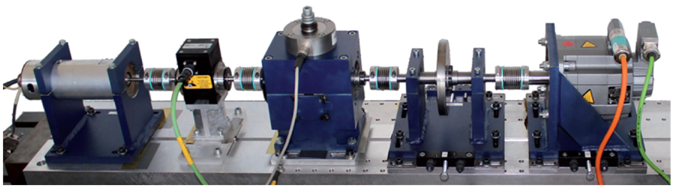
The PU bearing fault test rig.
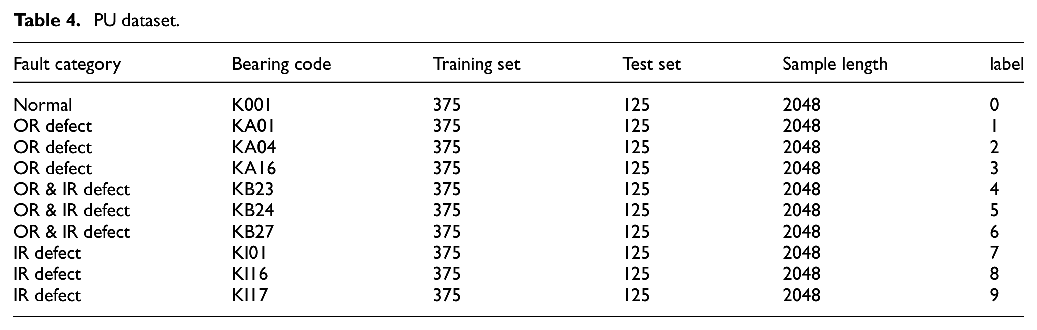
Four specific operating conditions—N15_M07_F10, N09_M07_F10, N15_M01_F10, and N15_M07_F04—were deliberately selected for the experiments. In this nomenclature, “N” represents the rotational speed, with N15 corresponding to 1500 rpm and N09 to 900 rpm. “M” denotes the torque magnitude, where M07 indicates 0.7 Nm and M01 represents 0.1 Nm. Additionally, “F” stands for the radial force, with F10 equating to 1000 N and F04 to 400 N. The rolling bearing data collected under these distinct operating conditions were systematically classified into four states: normal, inner race (IR) defects, outer race (OR) defects, and multiple defects involving both IR and OR defects, as outlined in Table 4.
PU dataset.
In this experiment, we also applied a sliding window overlap sampling method, as illustrated in equation (36), for data augmentation to prevent overfitting. The parameter
The loss values and accuracy curves during the training of the multi-scale CNN-Transformer model are shown in Figure 24. The confusion matrix on the PU dataset is presented in Figure 25. Figure 26 provides a T-SNE visualization of the features extracted by the multi-scale CNN-Transformer model. Figure 27 demonstrates the performance of different models using confusion matrices, highlighting the effectiveness of combining the Transformer network with the multi-scale CNN for fault diagnosis. Finally, Figure 28 offers a detailed comparison of the model’s performance using the four previously mentioned metrics.
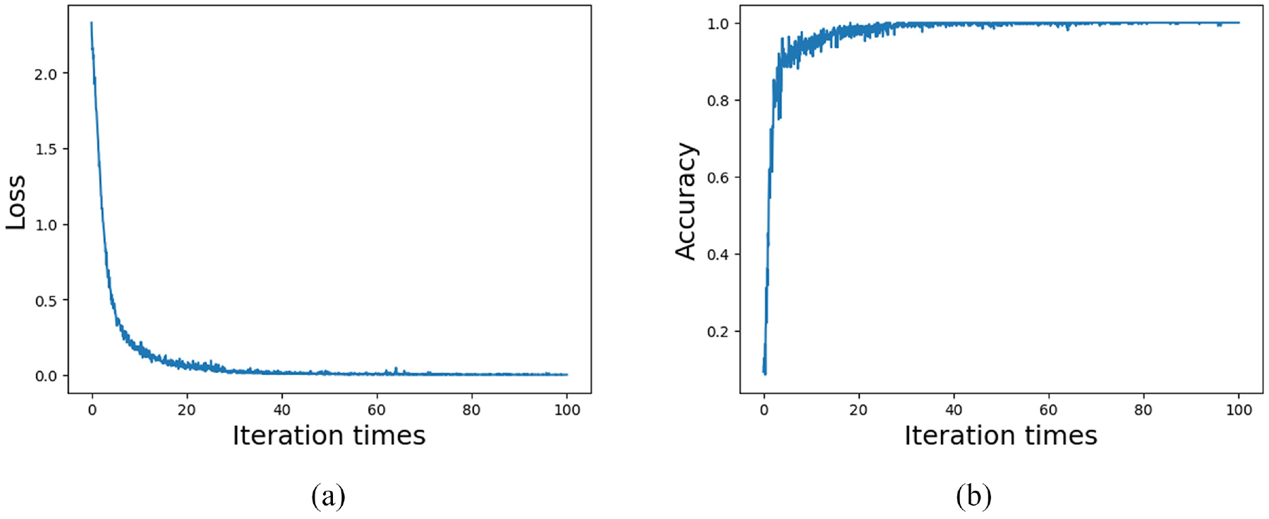
Loss values and accuracy curves of multi-scale CNN-Transformer model of the PU dataset: (a) loss curve and (b) accuracy curve.
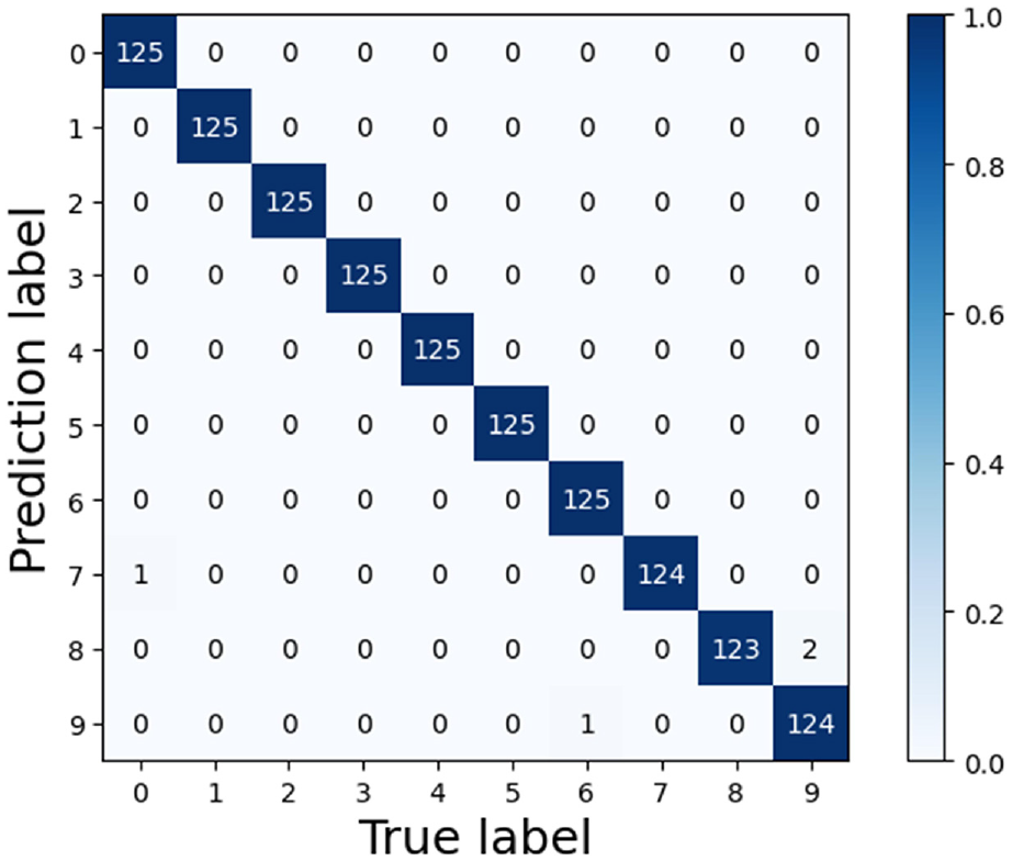
Confusion matrix of multi-scale CNN-Transformer of the PU dataset.
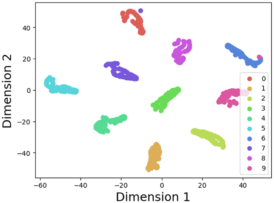
T-SNE visualization of the PU dataset.
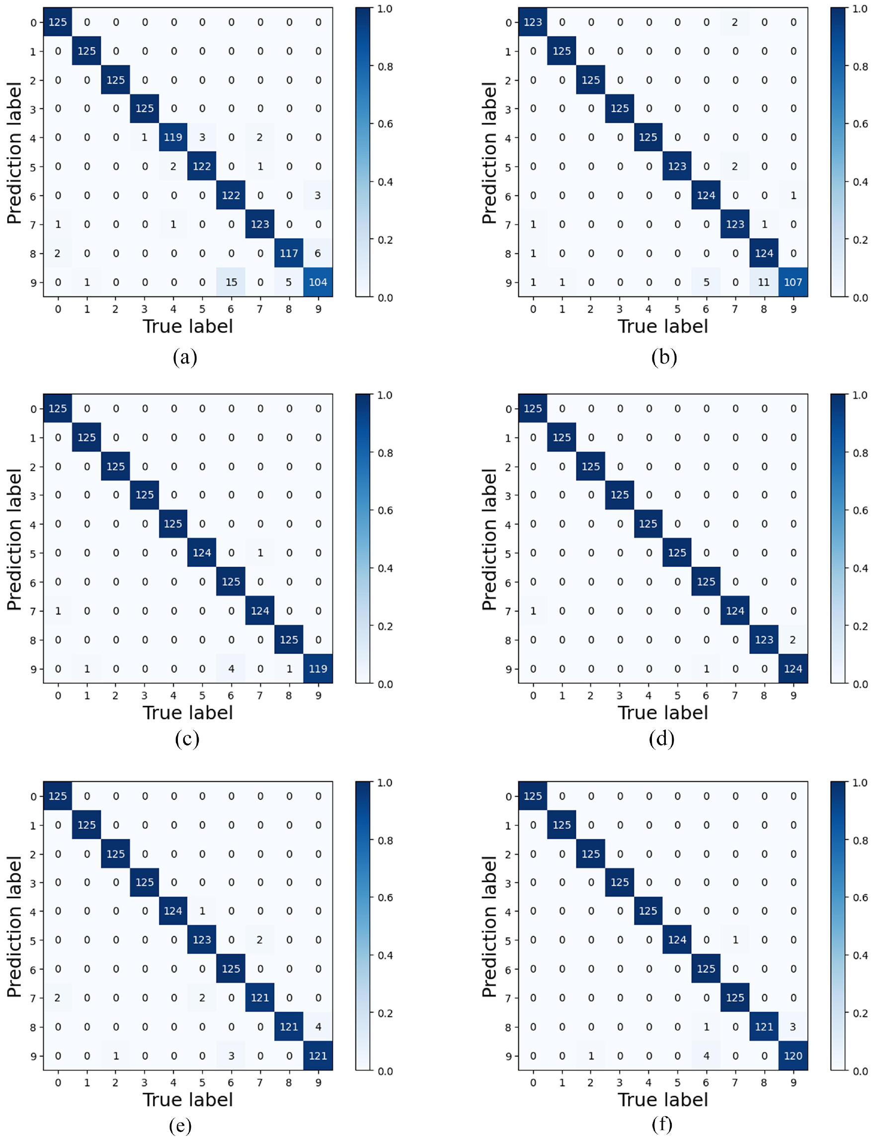
Confusion matrix of different model of the PU dataset: (a) CNN, (b) WDCNN, (c) CNN-Transformer, (d) multi-scale CNN-Transformer, (e) SNDCNN, and (f) MSCNN-LSTM.
Comparison of different methods using four performance evaluation metrics of the PU dataset.
Conclusions
This paper proposes an intelligent fault diagnosis method based on WOA-SVMD and multi-scale CNN-Transformer, which addresses the challenges of motor bearing vibration signals being easily interfered with by environmental noise and insufficient extraction of fault features. The WOA-SVMD method is used in the signal denoising process. WOA is employed to optimize the penalty factor parameter of SVMD, enabling the best signal decomposition. Then, the Pearson correlation coefficient method is applied to calculate the correlation between the IMFs obtained from the decomposition and the original signal. IMFs with low correlation are filtered out, while those with high correlation are retained to reconstruct the signal, achieving effective denoising. The feature extraction process employs a multi-scale CNN-Transformer model. The multi-scale CNN uses convolutional kernels of various sizes to extract local features from the input signal, constructing rich feature maps, and incorporates the ReLU activation function to enhance the network’s feature recognition capability. Subsequently, the Transformer is applied to capture global features through its self-attention mechanism. Finally, fault type is classified using the Softmax function. The proposed method has been validated on the CWRU and PU public datasets. Comparative experiments demonstrate that the method achieves superior signal denoising performance and higher fault diagnosis accuracy than other approaches.
However, fault diagnosis is only one aspect of machinery and equipment health management. In the future, we plan to test and optimize our models in the field of remaining useful life prediction of bearing.
Footnotes
Declaration of conflicting interests
The author(s) declared no potential conflicts of interest with respect to the research, authorship, and/or publication of this article.
Funding
The author(s) disclosed receipt of the following financial support for the research, authorship, and/or publication of this article: National Natural Science Foundation of China (62373321), Open Project of Zhejiang Key Laboratory of Automotive Electronics Intelligence (JY20240708) and National Key Laboratory of Industrial Control Technology (ICT2024B55).
Data availability statement
Data sharing not applicable to this article as no datasets were generated or analyzed during the current study.