
Abstract
Motivated by the thought of using couplings to reject disturbances, the authors propose a novel partial inverted decoupling control for improving the disturbance rejection of multivariable processes with time delays. With the relative disturbance gain (RDG) for n × n processes, whether the couplings among loops are favorable is evaluated. The inverted decoupling usually used in full decoupling control is then extended to partial decoupling control to retain the favorable couplings and remove the unfavorable ones. The elements of the partial inverted decoupler are derived and the implementation structure is provided. Based on the partially decoupled processes, the decentralized controllers for both the decoupled and non-decoupled loops are designed. An analytical design method for the decentralized controllers is proposed to improve disturbance rejection. Controller parameters are determined in terms of both performance and robustness. Two simulation examples show that the presented partial inverted control strategy can provide superior disturbance rejection to several other classical multivariable control strategies.
Introduction
In process control industries, most controlled processes are multivariable processes in nature. An important characteristic of multivariable processes is the couplings between the inputs and outputs. 1 Couplings make the control problem for multivariable processes much more complicated than that for univariate processes. Therefore, how to handle couplings is a key issue in multivariable control.
Decentralized control, with no doubt is the most commonly used control strategy for multivariable processes in practice due to its easy implementation. 2 The primary step for decentralized control is usually to determine the main channel of each loop. Therefore, how to pair the inputs and outputs so as to reduce relative couplings is of great importance 3 and many indicators have been proposed, such as relative gain array (RGA) 4 and some relevant methods with process dynamics considered.5,6 With the well-paired system, the decentralized controllers can be tuned by detuning method, 7 auto-tuning method 8 and iterative design method, 9 etc. Recently, Mahapatro et al. 10 designed decentralized PI controllers based on frequency response matching of a predefined reference model and the actual model. Mahapatro and Subudhi 11 proposed a robust decentralized PID controller based on complementary sensitivity function through a graphical tuning method. For minimizing the undesirable effects of the couplings, Euzébio et al. 2 optimized decentralized controllers by determining the cost function as the sum of the integral absolute errors (IAE) from each output due to set-point changes in coupled loops. Jeng and Lee 12 proposed a direct synthesis method for decentralized controllers on the basis of specifying the frequency response of the desired closed-loop transfer function matrix. Apparently, the decentralized controllers designed only with the main channels may not achieve sufficiently satisfactory control performances since the coupling information is ignored. As a result, the effective open-loop transfer function (EOTF) was proposed for independent design of multi-loop controllers. 13 In the formulation of the EOTF, the coupling channels were contained. With the concept of EOTF, the multivariable control system can be decomposed into several equivalent single-loops for decentralized controller design.14,15 However, since the calculation of EOTF is complex, especially for high-dimensional processes, model approximation is usually inevitable to simplify controller design. Approximation errors will affect the control performance. In sum, decentralized control cannot fully remove the effect of couplings in spite of its simple structure, which means it is suitable for the process with modest couplings.
When significant couplings exist, an intuitional way to improve control performance is to remove or reduce the loop couplings by inserting a decoupler. When the process is well decoupled, the control strategies for single-input-single-output (SISO) processes can be used directly. Hence, the design of the decoupler is the key issue in decoupling control. Generally, decoupling strategies are classified into two categories, that is, static decoupling and dynamic decoupling. 16 A static decoupler is designed by only considering the steady state of a process. It has the advantages of simple calculation and easy implementation while it may not provide satisfactory decoupling performance because of the neglected process dynamics. A dynamic decoupler can achieve better decoupling performance but it needs more accurate process information. As the most representative multivariable processes, many dynamic decouplers are firstly studied for 2 × 2 processes. Among them, the most classical three methods are ideal decoupling, simplified decoupling and inverted decoupling. 17 Ideal decoupling which uses the inverse of the process to design the decoupler is rarely used in practice because it suffers from complex decouplers. Compared with ideal decoupling, simplified decoupling is more popular as it provides a simple and implementable decoupler. However, a simplified decoupler usually results in a complex decoupled process, which is not desirable for controller design. This will be more evident when simplified decoupling is extended to high-dimensional processes. 18 Unlike the above two, inverted decoupling can achieve simple decouplers and decoupled processes simultaneously, but the limitations of achieving stable and realizable decoupler elements should be considered when it is applied for high-dimensional processes. 19 To overcome the effect of the mismatched model, Aguiar et al.20,21 proposed closed-loop evaluation and redesign methodologies for simplified decoupling and inverted decoupling. In essence, these dynamic decoupling methods seek to make the decoupled process matrix a diagonal matrix at more frequencies. Motivated by this, Jin and Liu 22 use the Nyquist set to describe the dynamics of the decoupler and use a complex-curve fitting technique to obtain an approximate decoupler matrix. Moreover, Xiong et al. 23 proposed the equivalent transfer function (ETF) based on the inherent relation between the inverse process and the dynamic relative gain array (DRGA) to simplify the design of the decoupler. Naik et al. 24 approximated the ETF using the static relative gains and the average residence time. Khandelwal and Detroja 25 presented a novel ETF parameterization procedure for large scale processes or systems with higher-order elements. To simplify the structure of multivariable system, the multivariable controller can have the abilities of both decoupling and control, which is called the centralized controller. Usually, a centralized controllers can be realized by combining a decoupler and a set of decentralized controllers. 26 Besides, a centralized controllers can also be synthesized directly based on a desired closed-loop transfer function matrix. 27 Garrido et al. 28 presented an iterative methodology for designing centralized PID controllers based on the proposed equivalent loop transfer functions. Gündeş 29 gave the necessary and sufficient conditions for the existence of decoupling controllers. Actually, the couplings can be regarded as the internal disturbances of the multivariable systems, which means the methods for handling couplings is to suppress the internal disturbances.
Apart from couplings, external disturbances and process uncertainties are inevitable in many industries, which makes the primary goal of the controllers to mitigate the effects of external disturbances and process uncertainties.30,31 Feedback control is an important strategy for suppressing disturbances. As the classical feedback controller, PID controller still dominates the engineering systems. The key issue of PID controller is to tune the controller parameters. The traditional tuning formula, such as Z-N method, are experiential methods, which are easy to implement while only achieve limited control performance. When the process model is known, the synthesis of PID controller can be transformed to solving the optimization problem with given objectives and constraints.32,33 With the development of machine learning techniques, some are incorporated to PID tuning to improve control performance such as neural network PID, 34 fuzzy PID 35 and swarm intelligent PID 36 , etc. To reduce the dependence of accurate models, data-driven techniques, like iterative feedback tuning 37 and virtual reference feedback tuning, 38 are employed to tune fix-structure controller, which is suitable for the processes with big uncertainties. Apart from feedback control, feedforward control is another effective scheme for disturbance rejection, which cancels disturbances with the reverses of disturbance signals. In light of the main drawback of feedforward control that it can only deal with measurable disturbances, many disturbance observers are designed to estimate the disturbances by using the measurable states and the process dynamics, which results in the disturbance observer-based (DOB) control. DOB control contains several related methods, such as frequency domain DOB control, 39 active disturbance rejection control (ADRC), 40 equivalent input disturbance (EID), 41 etc. Although under different names, these methods share the same basic idea, that is, the lumped disturbances including the external disturbances and uncertainties are estimated and corresponding compensations are generated based on the estimations. Due to realizing the compensation of uncertainties, DOB control does not require an accurate process model. 31 Meanwhile, its inherent 2 degree-of-freedom (DOF) structure allow the DOB control system to achieve a satisfactory performance in both set-point tracking and disturbance rejection. As a result, DOB control has been applied into more and more industries.42–44
As the typical characteristic of the multivariable system, the couplings can also be used for disturbance rejection when they have the opposite effect of the external disturbances. Motivated by this, Stanley et al. 45 defined the relative disturbance gain (RDG) to evaluate couplings for distillation processes. Similarly, Lin et al. 46 proposed the relative load gain (RLD) as the ratio of the gains of effective disturbances and open-loop disturbances. Moreover, Chang and Yu 47 systematically described the controller structure via internal model control (IMC) structure and proposed the relative disturbance gain array (RDGA) to synthesize the controller structure straightforwardly. Based on the evaluation of couplings, the partial decoupling structure can be constructed and some control strategies have been studied.48,49 As well, the thought of using couplings for disturbance rejection has been extended to other control structures.50,51
Motivated by the thought of using couplings to reject disturbances, this work is aimed to propose a novel partial decoupling control strategy. Unlike the existing methods which cannot remove the unfavorable couplings thoroughly due to the approximation or simplification of the decoupler, the proposed strategy extends the inverted decoupler which used in full decoupling control to partial decoupling control. The designed partial inverted decoupler can realize better elimination of the unfavorable couplings. Besides, in the existing methods, the controllers of the non-decoupled loops are usually designed based on the main channel models and disturbance channel models. The dynamic characteristics of non-decoupled loops are not analyzed sufficiently. In the proposed method, the equivalent process model and the equivalent disturbance channel model are obtained for designing the controllers of the non-decoupled loops. Finally, to simplify the design of the controllers, an analytical design method for the decentralized controllers is proposed by considering the performance of disturbance rejection and robustness. In sum, the main contributions of this work are concluded as follows:
(1) The RDG for general n × n processes is explored to evaluate whether the couplings are favorable or not.
(2) The inverted decoupling is extended to partial decoupling control to retain the favorable couplings and remove the unfavorable ones. The elements of the partial inverted decoupler are derived and the implementation structure is provided.
(3) The equivalent process models and the equivalent disturbance channel models are obtained to design the controllers of the non-decoupled loops.
(4) An analytical design method for the decentralized controllers is proposed with the consideration of both the performance of disturbance rejection and robustness.
This paper is organized as follows. In Section “Relative disturbance gain (RDG),” the RDG for general n × n processes is derived to evaluate the couplings. Based on the evaluation result, the design and implementation of the partial inverted decoupler are discussed in Section “Partial inverted decoupling control structure.” In Section “Design of the decentralized controller,” the decentralized controllers for decoupled and non-decoupled loops are designed respectively. An analytical design method is proposed. Two simulations examples are provided in Section “Simulation study.” Section “Conclusion” is the conclusion.
Relative disturbance gain (RDG)
With the purpose of using the couplings between loops to reject disturbances, the first but important step is to judge whether the couplings are favorable. Hence, an index for evaluating the couplings is necessary. With this index, the couplings beneficial to disturbance rejection should be retained while the unfavorable ones have to be decoupled. Herein, the index is chosen as RDG.
The RDG was proposed by Stanley et al. 45 for 2 × 2 processes, like dual-composition control. Equation (1) shows the definition of the RDG of the ith loop, that is, β i , where u i and y j are the input of the ith loop and the output of the jth loop, respectively; d is a disturbance signal.
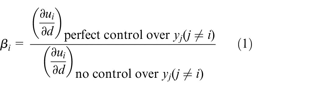
Obviously, β i is the ratio of the required input changes for rejecting the disturbances in two different cases. The numerator indicates the case where the decentralized control is used for the multivariable system while y j (j ≠ i) is under perfect control. In this case, the couplings are retained. The denominator indicates the case where the system has been well decoupled since y j (j ≠ i) has no effect on y i . Therefore, it can be concluded that the couplings are favorable to disturbance rejection if |β i | < 1, while harmful to disturbance rejection if |β i | > 1. According to equation (1), the expression of β i for n × n processes can be derived.
Figure 1(a) shows the commonly used decentralized control structure for general n × n processes, where C(s) is the decentralized controller, expressed as C(s) = diag(c1(s), c2(s), …, c
n
(s)); P(s) is the controlled process, whose element is described as p
ij
(s), i, j = 1, 2, …, n; L(s) is the disturbance transfer function vector, expressed as L(s) = [L1(s), L2(s), …, L
n
(s)]T;d(s) is a specific disturbance signal; r, u and y are the reference vector, input vector and output vector, respectively. Assuming that the loops have been paired, according to Figure 1(a), the ith disturbance response,
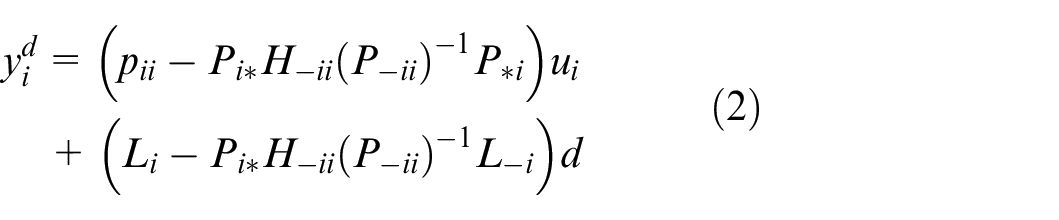
where

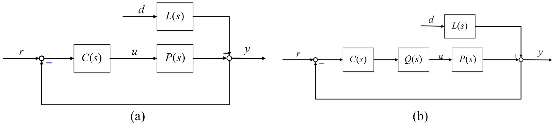
Control structures of multivariable systems: (a) decentralized control structure and (b) decoupling control structure.
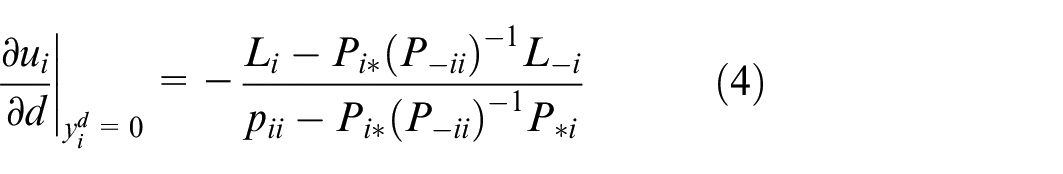
On the other hand, when a multivariable system is well-decoupled,
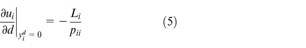
Based on equations (4) and (5), β i at steady state can be expressed as
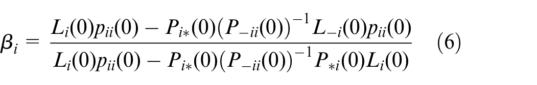
Next, β i will be used to evaluate the couplings, which is essential to determine the constitution of the partial inverted decoupler.
Partial inverted decoupling control structure
The basic decoupling control structure is shown in Figure 1(b). In Figure 1(b), the decoupler Q(s), between the controller and the process, is the main part to be designed. The partial inverted decoupling control shares the same structure with Figure 1(b). The primary step is to design the partial inverted decoupler.
Design of the partial inverted decoupler
In decoupling control, the decoupler can be synthesized directly in terms of the desired decoupled process,

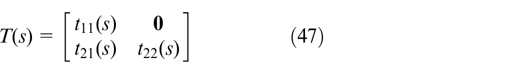
where T(s) is the desired decoupled process. For partial decoupling, T(s) here should be determined based on RDG. For n × n processes, assuming that there are m (m ≤ n) loops with unfavorable couplings, the process transfer function matrix can be reformed as
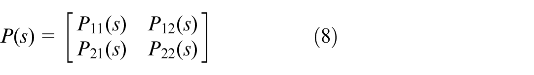
where P11(s), P12(s), P21(s), and P22(s) are an m × m, m × (n−m), (n−m) × m and (n−m) × (n−m) matrix, respectively. Since the first m loops need decoupling, the decoupled process should have the following form,
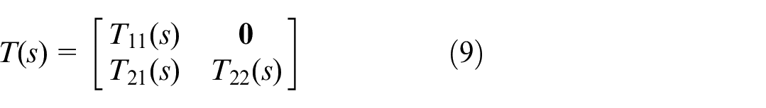
where T11(s) = diag{t1(s), t2(s), …, t m (s)}. To facilitate analysis, the decoupler matrix Q(s) is written as a block matrix, that is,
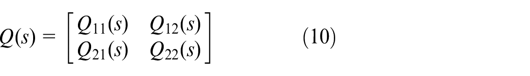
The design of Q(s) is transformed to determine Q11(s), Q12(s), Q21(s), and Q22(s). In view of T(s) = P(s)Q(s), the following equations can be obtained:
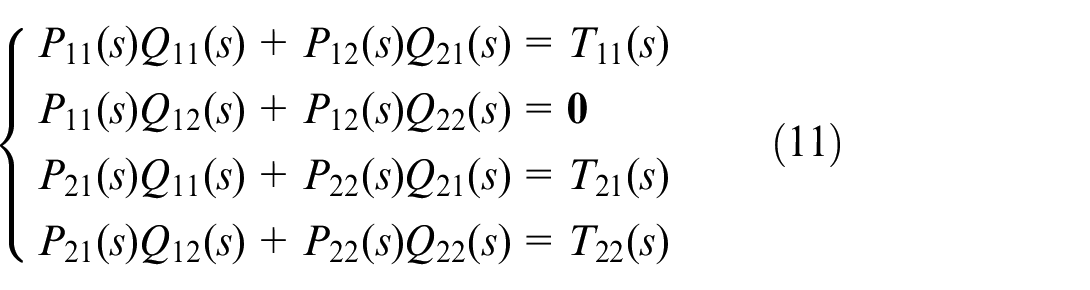
Considering that there are (n−m) loops using decentralized control, let Q21(s) =
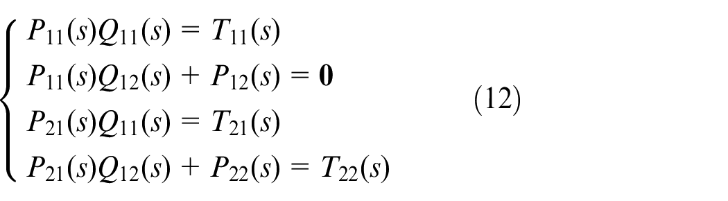
where the remaining undetermined parts are Q11(s) and Q12(s). According to equation (12), it is obvious that
Structure of inverted decoupling.
where Q11(s) is realized by two parts, that is, V1(s) and V2(s). According to Figure 2, Q11(s) can be expressed as

Substituting

Since T11(s) is a diagonal matrix, it is straightforward to compute its inverse. Similarly, V1(s) should be determined as a diagonal matrix, that is, V1(s) =diag{δ1(s), δ2(s), …, δ m (s)}. For further simplification, V2(s) is determined as
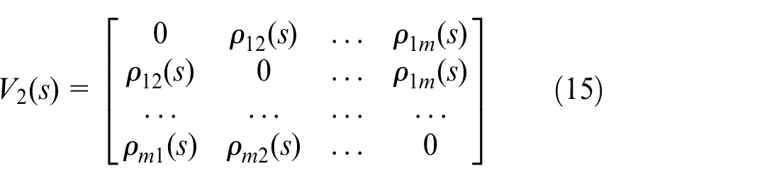
To satisfy equation (14), the elements of V1(s) and V2(s) should satisfy
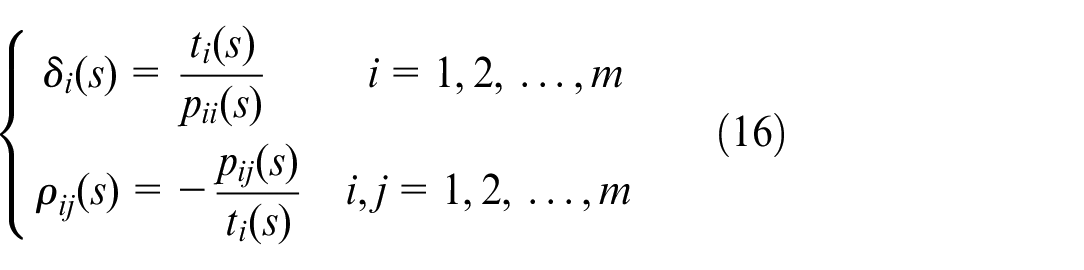
Equation (16) shows that the elements of V1(s) and V2(s) rely on the selection of the elements of T11(s).
After determining Q11(s), the design of Q12(s) will be undertaken. In light of equation (12) and Q11(s), Q12(s) is derived as

where
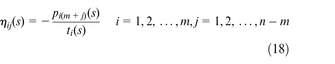
Obviously, the elements of V3(s) are also related to the elements of T11(s). Therefore, how to determine T11(s) needs a discussion.
The principle of determining T11(s)
The above procedure reveals that the partial decoupler can be accomplished after T11(s) is determined. However, considering the realizability of V1(s), V2(s), and V3(s), there are some constraints for the elements of T11(s). Concretely, the elements of V1(s), V2(s), and V3(s) should be causal, proper and stable, which results in the constraints for the time delay, relative degree and right-half-plane (RHP) zeros of t i (s).
Constraint for the time delay
Equations (16) and (18) show that each element of V1(s), V2(s), and V3(s) is a ratio of two transfer functions. Hence, to make sure the elements of V1(s), V2(s), and V3(s) are causal, the time delay of t i (s) should satisfy
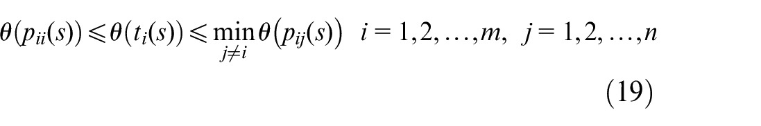
where θ(x) is the time delay of a transfer function x(s).
Constraint for the relative degree
Similarly, the elements of V1(s), V2(s), and V3(s) will be proper if they have nonnegative relative degrees. Hence, the relative degree of t i (s) should satisfy
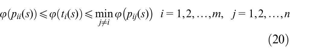
where φ(x) is the relative degree of a transfer function x(s).
Constraint for the RHP zeros
Moreover, the elements of V1(s), V2(s), and V3(s) should be stable. Therefore, the numerator and denominator in equations (16) and in (18) should have the same RHP zeros and the multiplicity of each zero should satisfy
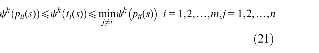
where ψ k (x) is the multiplicity of the kth zero of a transfer function x(s).
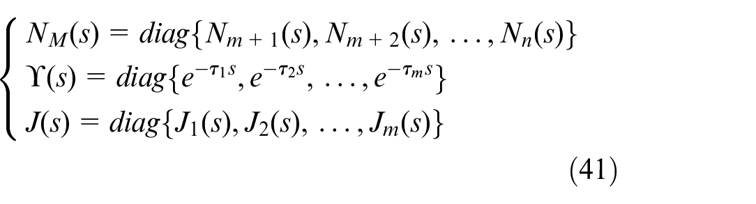
From Inequalities (19) to (21), it can be seen that p ii (s) should have the smallest values in terms of time delay, relative degree and multiplicity of RHP zero in the ith row. However, the original process matrix in equation (8) may not meet these requirements. If so, the process matrix P11(s) can firstly be reformed by interchanging the rows to meet these requirements. Unfortunately, in some cases, reformation may make no difference for the above problem. An effective solution is to introduce a compensator expressed as equation (22) to modify the characteristic of the process.
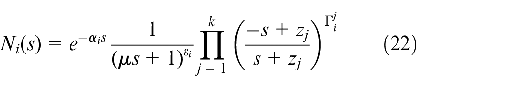
N
i
(s) is the compensator inserted in the ith loop and it is composed of three parts, which are used to compensate the time delay, relative degree and multiplicity of RHP zero, respectively. In equation (22), μ is a positive real constant; z
j
denotes the jth RHP zero; α
i
, ε
i
and
where x
i
can be parameter α
i
, ε
i
or
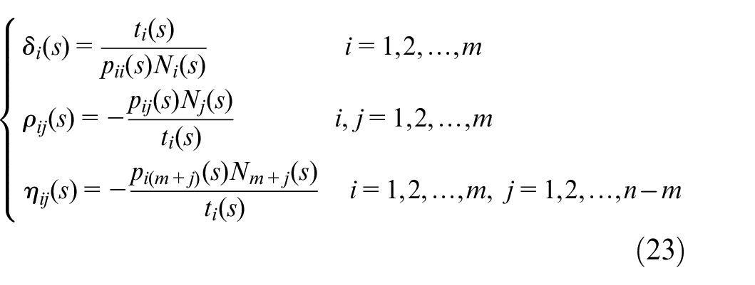
Finally, it is time to determine t i (s) to finish the design of V1(s) V2(s), and V3(s). Given the constraints of t i (s), an intuitive and simple selection is t i (s) = p ii (s)N i (s). This selection can result in the simplest form of V1(s), that is, V1(s) = I. Certainly, this is not the only way to select t i (s). Sometimes, other simpler forms of t i (s) are also available, but they will undoubtedly complicate V1(s). With t i (s) = p ii (s)N i (s), the elements of V2(s) and V3(s) can be derived accordingly as
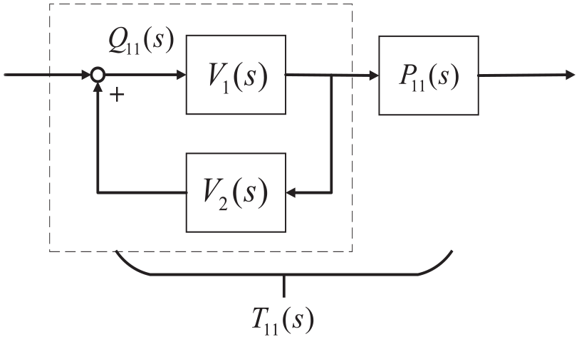
In the end, the implementation structure of the partial inverted decoupling control is shown in Figure 3, where C d (s) and C m (s) are the decentralized controller matrix of decoupled loops and non-decoupled loops, respectively; L d (s) and L m (s) are the disturbance transfer function vector of decoupled loops and non-decoupled loops, respectively; Y d (s) and Y m (s) are the output vector of decoupled loops and non-decoupled loops, respectively; R d (s) and R m (s) are the reference vector of Y d (s) and Y m (s), respectively.
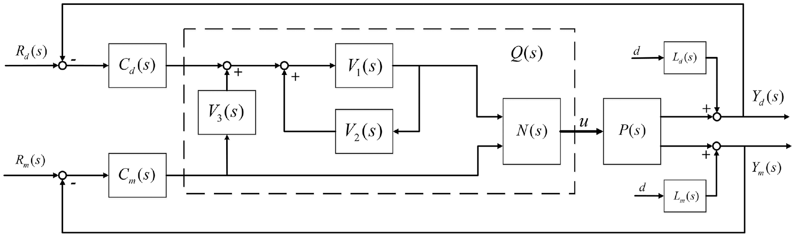
Implementation structure of partial inverted decoupling.
In Figure 3, the decentralized controllers C d (s) and C m (s) are still the unknown parts, which will be studied in the next section.
Design of the decentralized controller
Decentralized controllers C d (s) and C m (s) are located in the decoupled loops and the non-decoupled loops, respectively, to improve the performance of disturbance rejection. The design of C d (s) and C m (s) will rely on the partially decoupled process. According to Figure 3, the disturbance response [Y d (s), Y m (s)]T can be expressed as
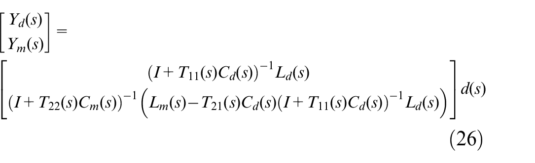
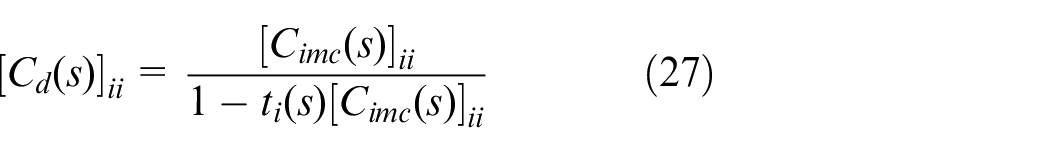
From equation (26), it can be observed that Y d (s) is only related to C d (s) while Y m (s) is determined by both C d (s) and C m (s). Thus, the decentralized controllers C d (s) and C m (s) should be designed in sequence. Firstly, C d (s) will be designed by optimizing Y d (s). And then the design of C m (s) can be undertaken for optimizing Y m (s) with the determined C d (s).
Design of the controllers in the decoupled loops
As the couplings in the decoupled loops have been removed, the decoupled system can be regarded as a series of independent subsystems. The ith element of C
d
(s),
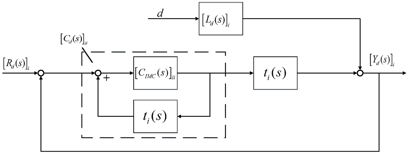
Internal model control structure of the ith subsystem.
According to the IMC structure, the disturbance response

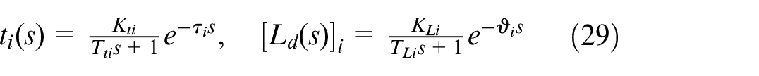
where t
i
(s) and
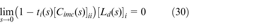
Assuming d(s) = 1/s, the necessary condition for steady-state performance of disturbance rejection is
Based on equation (30) and IMC principle, the potential internal model controller can be designed as

where
From equation (28), obviously, if slow modes exist in the disturbance channel, the performance for disturbance rejection will be deteriorated. To speed up disturbance rejection,
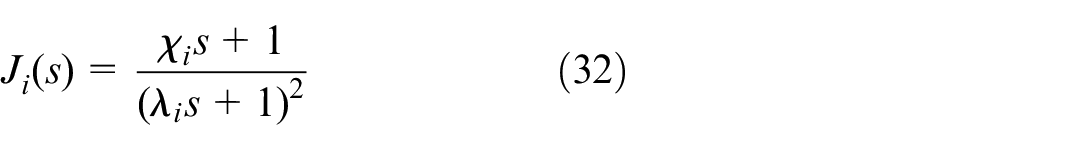
In order to eliminate the slow mode, the undesired poles of
The proof of equation (33) is shown in the Appendix.
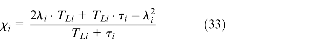
From equation (33), χ
i
can be calculated when a concrete λ
i
is given. Hence, the selection of λ
i
will be focused on next. Obviously, in terms of speeding up disturbance rejection, a small value of λ
i
is preferable. Meanwhile, a small value of λ
i
can also provide a small gain for the disturbance output, which can suppress the peak value of the disturbance output (The gain of disturbance output can be approximately described as

A large value of M s reveals bad robustness and a typical range of M s is [1.4, 2.0]. For ease of analyzing the relationship between λ i and M si , define Λ i = λ i /T Li , Ξ i = T Li /τ i , and Ω i = ω·τ i , where ω is the frequency. Then, M si in equation (34) can be rewritten as
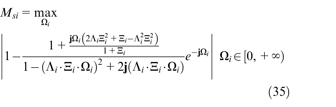
where
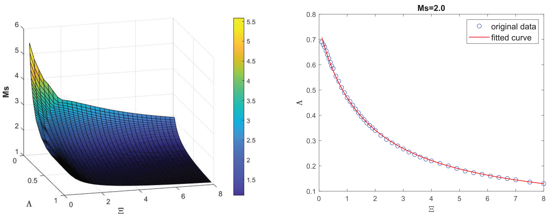
Relationship between system parameters and M s : (a) relationship between Λ, Ξ and Ms and (b) relationship between Λ and Ξ for M s = 2.0.
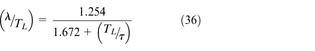
According to Figure 5(a), for a specific Ξ, M s decreases while Λ increases. This reveals that a large λ (Λ) can improve the robustness. Therefore, with respect to the selection of λ, there is a tradeoff between robustness and performance. Meanwhile, for a specific Λ, M s decreases while Ξ increases. In light of this, it can be inferred that if a system has a relatively large time delay, controller parameter λ ought to be increased to guarantee sufficient robustness. Figure 5(b) shows the relationship between Λ and Ξ for M s = 2.0 and an approximate expression has been obtained as equation (36). In this way, the value of M s will lie in the typical range, when λ ≥ 1.254T L /(1.672 + T L /τ).
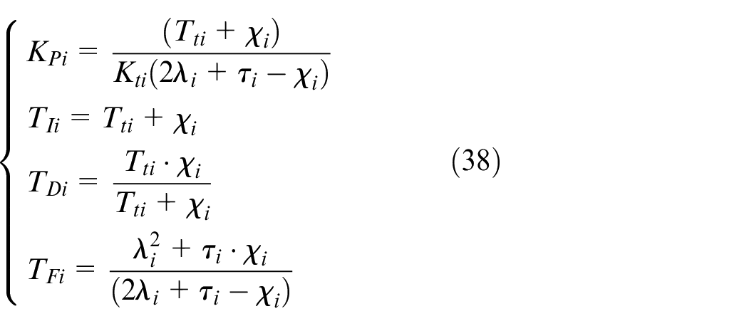
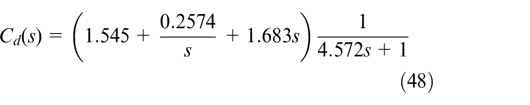
The design of internal model controller can be finished along with the determination of λ i . Furthermore, based on equation (27), the equivalent feedback controller which is in the form of a PID controller can be fulfilled as
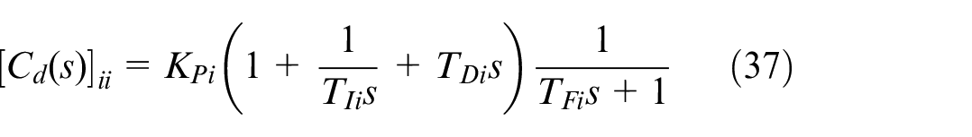
where
Design of the controllers in the non-decoupled loops
After C d (s) is obtained, the decentralized controllers in the non-decoupled loops, C m (s) will be designed then. Similarly, the disturbance output Y m (s) can be denoted as

where L e (s) and T22(s) are the equivalent disturbance channel model and the equivalent controlled process model, respectively. L e (s) and T22(s) have the following expressions:
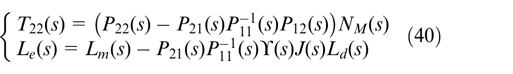
where
According to equation (39), the design of C m (s) relies on L e (s) and T22(s). For the independent design of the decentralized controllers, the idea of EOTF is used. 13 The EOTFs of the process model and disturbance model are
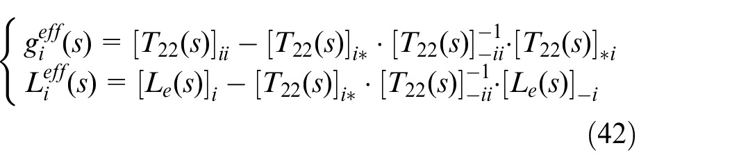
where
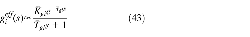
where
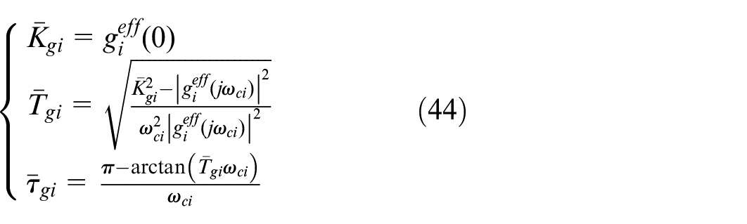
and ω
ci
is the phase cross-over frequency of
Simulation study
In this section, two examples are provided to demonstrate the effectiveness of the proposed method.
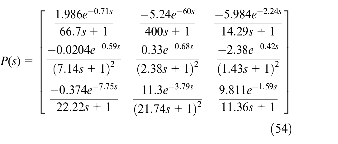
The process transfer function matrix of ISP reactor is
The disturbance transfer function vector is assumed to be
First, the couplings should be evaluated based on RDG. According to equation (6), the values of RDG are computed as |β1| = 1.069 and |β2| = 0.1357, which indicates that the couplings in loop 1 need to be removed while the couplings in loop 2 need not. Therefore, the decoupled process is determined as
Then, t11(s) will be determined to design the components of the partial inverted decoupler, that is, V1(s), V2(s), and V3(s). Fortunately, p11(s) meets the requirements given in Section “The principle of determining T11(s),” which means the extra compensation is unnecessary. In this case, N(s) = I and t11(s) = p11(s). Substituting t11(s) into equations (16) and (18), the components are obtained as V1(s) = 1, V2(s) = 0 and V3(s) =
For the non-decoupled loop, C
m
(s) can be designed with the approximately equivalent models
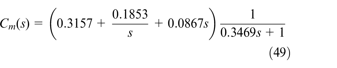
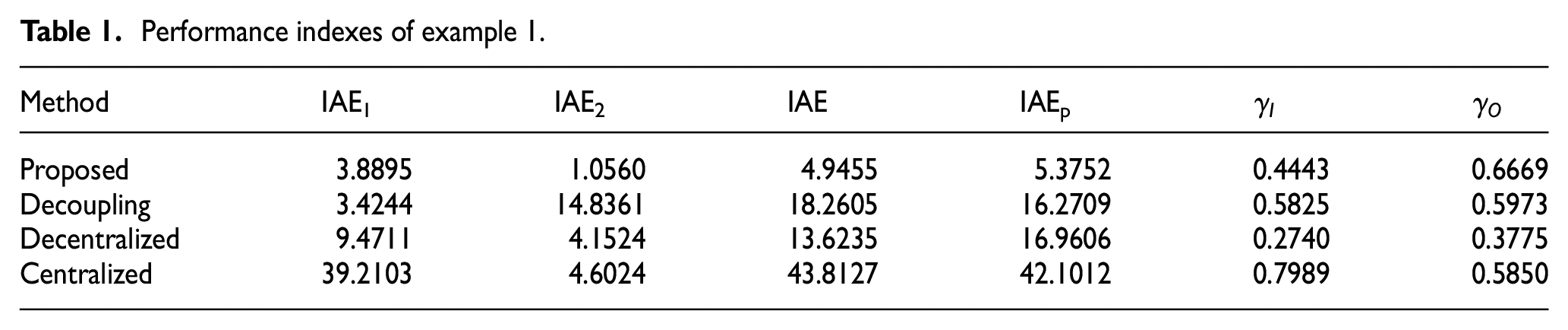
with λ m 1 = 0.3 for better robustness. With the decentralized controllers, the output response is shown in Figure 6(a). The proposed method is compared with several classical control strategies for multivariable processes, such as decentralized control, 52 centralized control 53 and decoupling control. 22 In Figure 6(a), it can be seen that the proposed method can achieve better performances for disturbance rejection. The peak of disturbance outputs of the proposed method are smaller. Meanwhile, the proposed method can bring the outputs back to their set-points in shorter time, especially in loop 2. Moreover, the integral absolute error (IAE) defined as
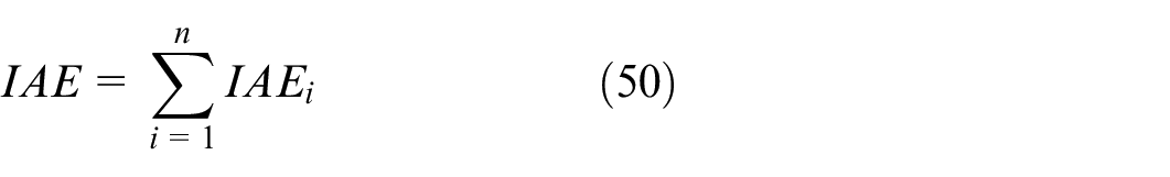
where
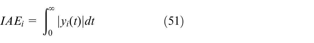
is also used to evaluate the control performance. The IAE values of different control strategies are listed in Table 1 for comparison. It is noticed that the smallest IAE value is provided by the proposed strategy. In addition to the nominal control performance, it is also important to evaluate the robustness of the control system. Therefore, +20% parameter perturbations are introduced to the controlled process to evaluate the robust performance. Figure 6(b) depicts the disturbance outputs of the system with parameter perturbations. It can be seen that the proposed method can keep the better performances in terms of the output peak, response time and IAE value (The IAE values of the perturbed system are also listed in Table 1 and denoted by IAEp). Then, the robust stability will be evaluated. For a multivariable system, both input uncertainty and output uncertainty should be considered. According to the M-Δ structure, in order to ensure robust stability, the multiplicative input uncertainty Δ I (s) and the multiplicative output uncertainty Δ O (s) should satisfy
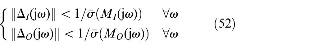
where
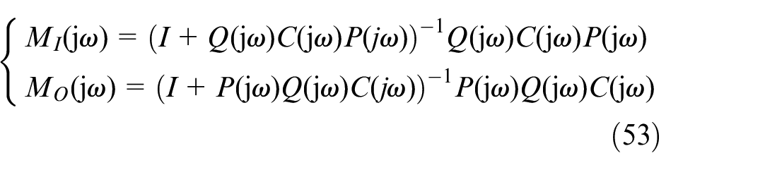
and C(s) = diag{C
d
(s), C
m
(s)}. The curves of
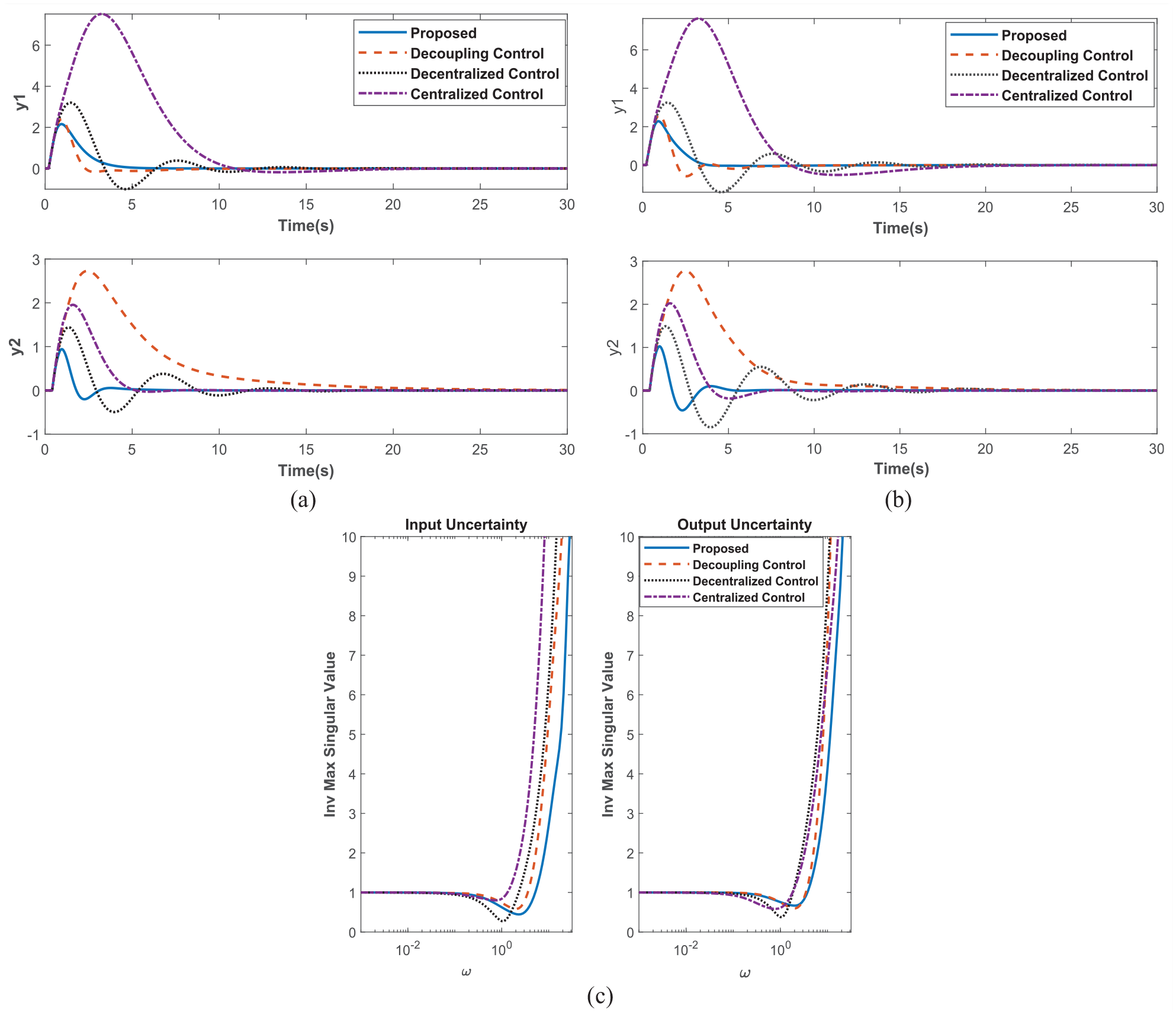
Control performance for example 1: (a) output responses for example 1 on nominal condition, (b) output responses for example 1 on perturbed condition, and (c) curves of 1/||M(jω)|| for example 1.
Performance indexes of example 1.
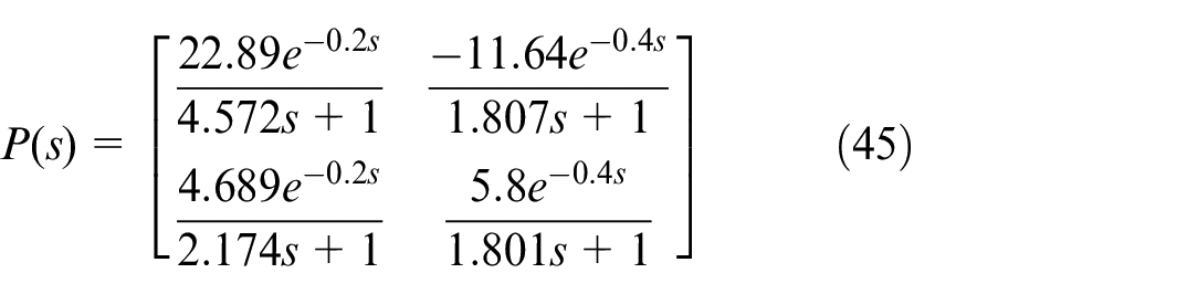
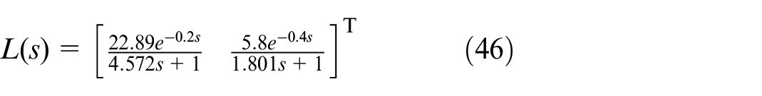
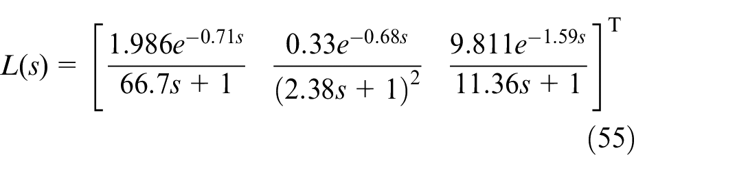
Here, a widely-studied 3 × 3 industrial distillation column is considered as
with an assumed disturbance transfer function vector
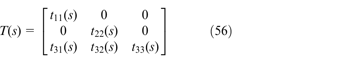
First, RDGs are calculated as |β1| = 3.5827 and |β2| = 1.0120 and |β3| = 0.0290 to evaluate couplings. Consequently, the couplings of the first two loops need to be removed while that in the last loop need not. As a result, the decoupled process is determined as
In this case, a compensator designed as N(s) =diag{e−0.09s, 1, e−0.26s} is needed as the requirement for the time delay cannot be met if t11(s) = p11(s) and t22(s) = p22(s) are selected directly. Based on the compensated process, V1(s), V2(s), and V3(s) are achieved as V1(s) = I,
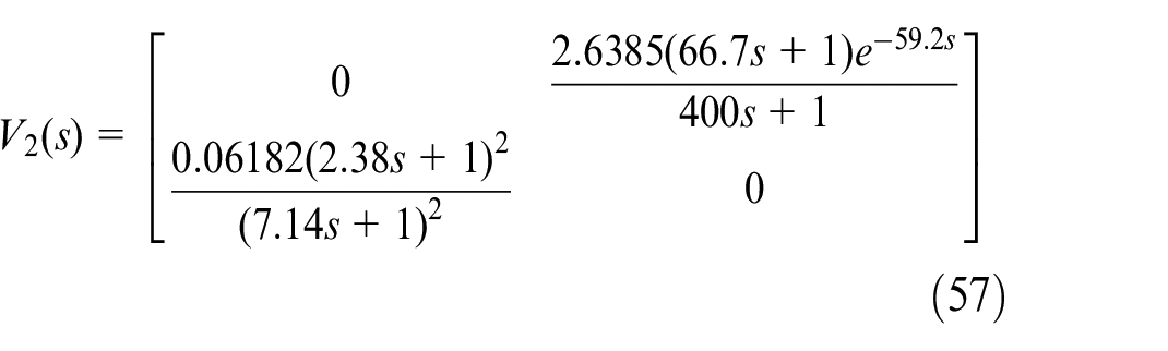
and V3(s) =
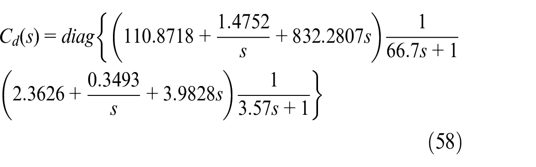
Then, the controller of the non-decoupled loop, C
m
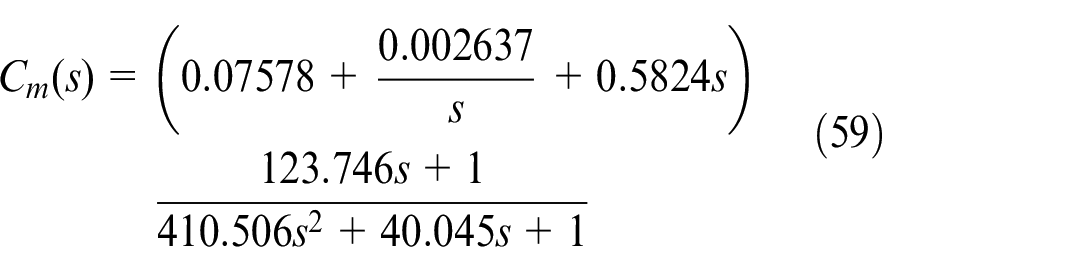
(s) is designed based on the approximate equivalent models,
The output responses of the nominal process are shown in Figure 7(a) compared with Liu’s
54
analytical decoupling control strategy, ETF-based partial decoupling control strategy
49
and controller synthesis based on RDGA.
47
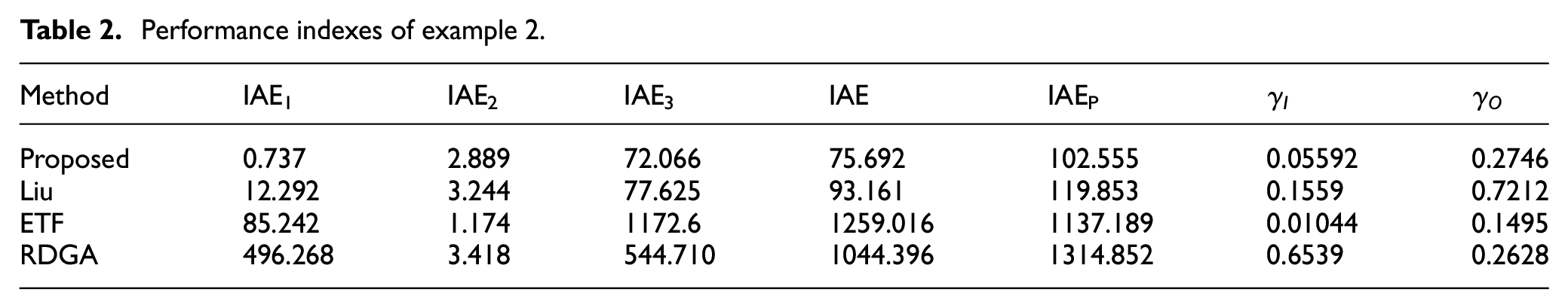
The corresponding IAE values are listed in Table 2. Obviously, the proposed method provide better output performances than other methods. Similarly, to evaluate robust performance, −20% parameter perturbations are introduced to the controlled process and the corresponding output responses are depicted in Figure 7(b). The proposed method can still achieve the best IAE value for the perturbed process. Besides, the curves of
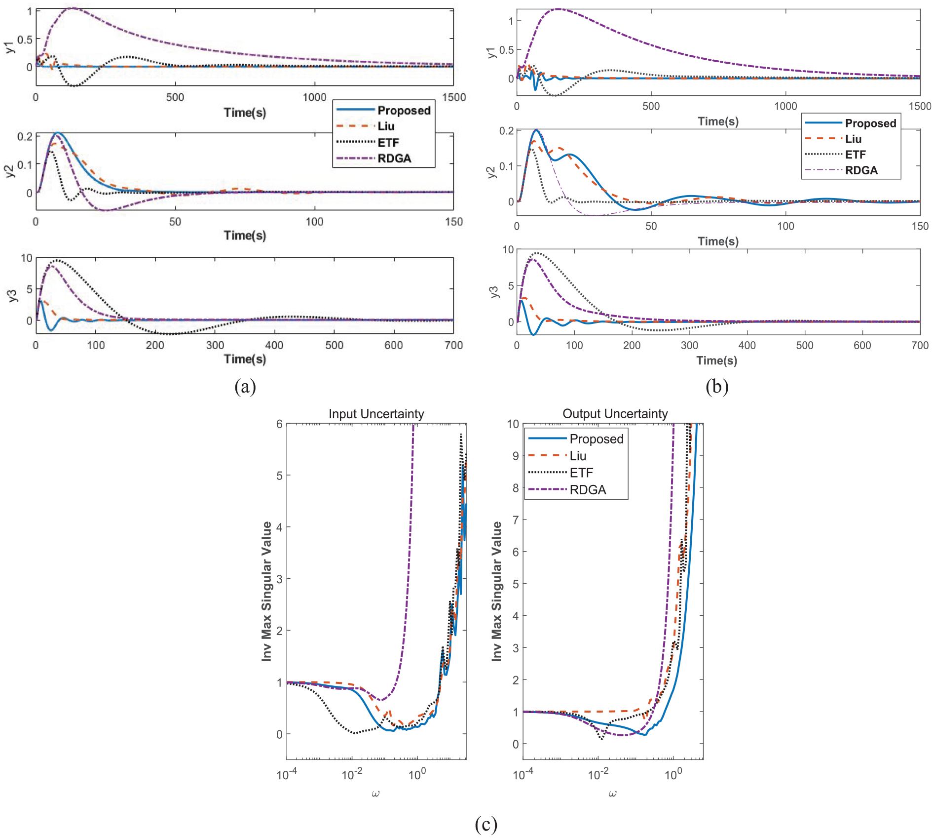
Control performance for example 2: (a) output responses for example 2 on nominal condition, (b) output responses for example 2 on perturbed condition, and (c) curves of 1/||M(jω)|| for example 2.
Performance indexes of example 2.
Conclusion
In this work, a novel partial inverted decoupling control strategy to improve the disturbance rejection of multivariable process with time delays is presented. Two main issues: the design of the partial decoupler and the decentralized controllers, are focused on. Motivated by the thought of using favorable couplings to reject disturbances, the couplings are firstly evaluated with RDGs. Then the inverted decoupling usually used in full decoupling control is extended to partial decoupling control. The elements of the partial inverted decoupler are designed in detail and the implementation structure is presented. The advantage of the proposed partial inverted decoupler is that the decoupler is implemented without approximation, which can remove the unfavorable couplings thoroughly. Based on the partial decoupled processes, the decentralized controllers for both the decoupled and non-decoupled loops are designed. An analytical design method is proposed with due consideration of the performance of disturbance rejection and robustness. Moreover, to improve the control performance of the non-decoupled loop, the equivalent process model and the equivalent disturbance channel model are obtained for controller design. Two simulation examples are provided and the results show that the proposed method can achieve better nominal control performance and robustness compared with several existing multivariable control strategies.
Footnotes
Appendix
Substituting equations (29), (31), and (32) into equation (28), the transfer function from d(s) to
Using the first-order Taylor approximation,
To cancel the undesired pole of
Equation (33) can be obtained based on equation (A.3).
Declaration of conflicting interests
The author(s) declared no potential conflicts of interest with respect to the research, authorship, and/or publication of this article.
Funding
The author(s) disclosed receipt of the following financial support for the research, authorship, and/or publication of this article: This work is supported by the National Natural Science Foundation of China [62003152] and Xuzhou Science and Technology Project of China [KC23008].
Data availability statement
Data sharing not applicable to this article as no datasets were generated or analyzed during the current study.