Sage Journals: Discover world-class research

Abstract

Aiming at the limited fitting conditions of existing 3D circle feature extraction algorithms, a 3D circle feature extraction algorithm based on nonparametric estimation is proposed. Firstly, kd-tree is used to establish topological relationship and define the distance threshold. Edge points are extracted by K-nearest neighbor search. Then use DBSCAN (Density-Based Spatial Clustering of Applications with Noise) to cluster edge points for calculate the maximum distance between edge points in the cluster. Finally, the optimal interval of the maximum distance value is calculated using nonparametric estimation. The center point is obtained by extracting the circular hole feature points. The degree of dispersion from the edge point in the cluster to the center point is analyzed to determine whether the cluster is a three-dimensional circle feature. The algorithm is verified using the grid assembly printed parts (arch circular hole) and rectangular flange (plane circular hole) as the test workpiece. The results show that the algorithm can effectively extract three-dimensional round hole features.

Keywords

Circle feature extraction edge extraction kd-tree DBSCAN nonparametric estimation

Introduction

Reverse engineering has become increasingly popular in industrial inspection in recent years. The point cloud data of workpiece is usually collected using laser scanning, and the non-contact detection of the workpiece is completed through data processing.^1–3 The 3D circle feature in the point cloud model is an essential geometric characteristic with substantial research implications for model reconstruction and reverse engineering. As a result, the point cloud model circle feature extraction has both theoretical and practical utility.^4–8

Some researchers extract model features using local neighborhood characteristics and geometric properties of point clouds to perform feature extraction in point cloud models. Shi and Wang⁹ constructed boundary point set removal and merging criteria as well as candidate feature point set smoothing criteria to identify feature points from boundary point sets of each segment. However, the recognition process of the method is more difficult for locations with weak feature strength. Xue et al.¹⁰ used the least square fitting method to recognize the feature of the three-view slices of the point cloud model. When the point cloud distribution was uneven, the detection accuracy of the point cloud model will be affected. Demarsin et al.¹¹ used the first order segmentation to extract candidate feature points, and recovered the sharp feature lines by visually processed. But this approach cannot operate effectively in distributed point cloud models. Wang et al.¹² segmented point cloud data using a clustering technique and extracted point cloud feature information in each subregion with defined bounds. However, the feature line extraction is still broken or partial in the point cloud model with additional curve feature information. For multiparameter K-means clustering, Wang et al.¹³ presented an adaptive point cloud reduction technique. In the closed model, the approach has a considerable simplification effect. But the computation of characteristic parameters was complicated. Deep learning had been used to extract edges and recognize holes in point clouds by Tabib et al,¹⁴ Qi et al,¹⁵ Wang et al,¹⁶ Bazazian et al,¹⁷ Zhang et al.¹⁸ When processing large-scale point cloud data, this approach required high computer performance.

This paper offers a 3D circle feature extraction approach based on nonparametric estimation to address the concerns of the aforementioned point cloud feature extraction accuracy and constrained fitting conditions. Distance density analysis is used to extract the edge point set, DBSCAN (Density-Based Spatial Clustering of Applications with Noise) is used to achieve edge point clustering. When the number of clusters to be formed is unknown, DBSCAN can recognize clusters of arbitrary shape in noisy environments, and the order of data input has little effect on the results. Nonparametric estimation is used to provide the ideal interval of the maximum distance value, and feature points are extracted for circular feature identification. The detection process is outlined in Figure 1.

Figure 1.

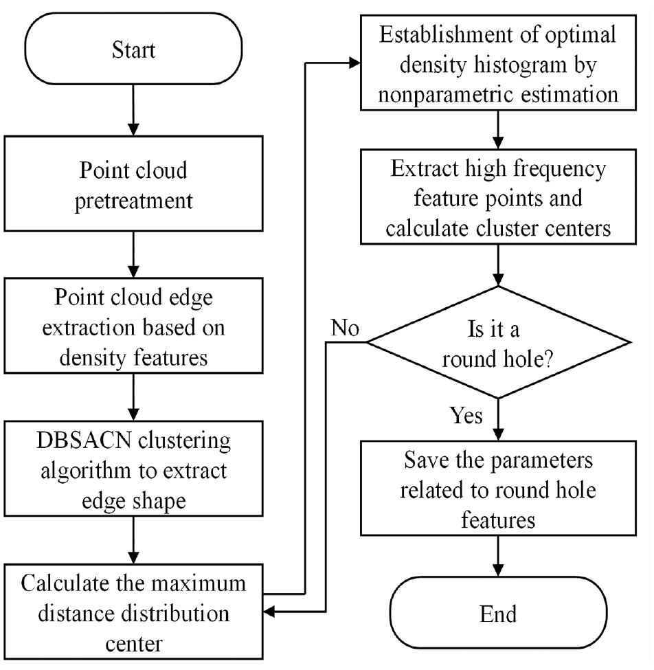
3D round hole feature detection process.

Point cloud model preprocessing algorithm

The preprocessing of point cloud model is a key step in detection. The purpose is to simplify the point cloud data and improve the computational efficiency and detection accuracy on the premise of maintaining the geometric characteristics of the point cloud. The topological relationship is established to realize the data indexing and denoising of 3D point cloud.

Establishment of topological relationships

3D point cloud is irregularly distributed in space and has no positional relationship. In the process of hole edge extraction and recognition, it is necessary to create point cloud data index and point cloud topology relationship to improve the processing efficiency of point cloud model. The kd-tree approach is utilized to build the spatial topological relationship of point clouds in this article, and K-Nearest Neighbor (KNN) is used to find the k-nearest neighbor.¹⁹

Extraction of point cloud edges

When the line laser is scanning and modeling, there are typically noise spots due to interference from the surroundings. To prepare for future point cloud feature extraction, point cloud noise reduction is required during the preprocessing stage. In this study, radius filtering and statistical filtering are employed to deal with discrete point cloud noise.

The primary goal of point cloud edge extraction is to eliminate unnecessary points and save calculation time. The point set P = {p_i | p_i $\in$ R³, i = 1,2,3,⋯,N} is created after creating the kd-tree spatial topological relationship, the K-nearest neighbor search on the point p_i is done using KNN, and the k points closest to the point p_i’s Euclidean distance are preserved in the set N(p_i). The edge extraction effect is best after several attempts when the value of k is 30. The algorithm works in the following manner:

Calculate the density of a point cloud

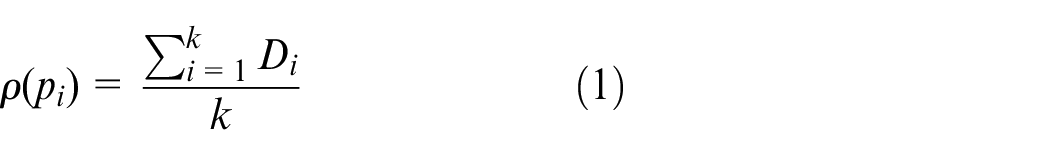
After searching for the nearest k points of all points with KNN, compute the distance D_i between point p_i and its nearest k points, and then average them all to obtain the point cloud density ρ(p_i). This is shown in (1):

ρ (p_{i}) = \frac{\sum_{i = 1}^{k} D_{i}}{k}

(1)

Set the distance threshold

The distance threshold n is calculated using (2)

n = μ \times ρ (p_{i})

(2)

where u is the threshold coefficient. To adjust the threshold n,

(1) Set the threshold coefficient μ and calculate the distance threshold n.

(2) Perform edge recognition and effect display.

(3) Using the edge extraction effect as a guide, adjust the threshold coefficient μ to produce the ideal threshold n with the best extraction effect.

Extraction of point cloud edges

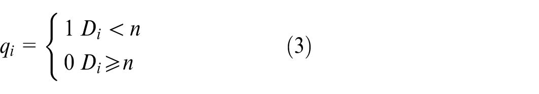
Find each point p_i and its nearest k points, compute the distance D_i between point p_i and its nearest k points, and find a value larger than the threshold n in D_i (i = 1,2…,k). The edge point q_i (x,y,z) corresponding to the distance D_j is designated as the distance point D_j and saved in a new point set E(q_i). The interior points are allocated a value of 1, while the edge points are assigned a value of 0. This is shown in (3):

q_{i} = {\begin{matrix} 1 D_{i} < n \\ 0 D_{i} \geq n \end{matrix}

(3)

Update the threshold coefficient

After traversing all the points and identifying the edge points, the edge points are visualized, and the effect of edge extraction is analyzed. If the edge extraction is not obvious, return to Step (2) and adjust the value of the threshold coefficient μ.

Cluster analysis of point clouds

After acquiring the edge dataset E(q_i), the DBSCAN technique is used to perform clustering analysis on the data to efficiently categorize edge points and decrease the computation of circular feature extraction E(q_i).²⁰

In the DBSCAN algorithm, there are two important parameters: epsilon and Minpts, where epsilon is the neighborhood radius when defining the density, and Minpts is the minimum number of data points within the radius of the sphere. The algorithm principle is as follows:

Step1 Randomly select data points e_i, set the neighborhood radius epsilon, and the threshold Minpts of the number of data objects in the neighborhood;

Step2 Take the data point e_i as the center, search for points within the epsilon, and determine whether the number of points is greater than or equal to the Minpts, if so, the point e_i is determined to be an in-cluster point; otherwise, it is excluded;

Step3 When e_i is the point in the cluster, and the rest of the points in the radius of the sphere are the center, repeat Step2, and repeat the judgment process for the points that meet the judgment;

Step4 After a round of search is completed, all points that meet the judgment are grouped into one category. Reselect unclassified points for judgment, and iterate until all points are classified.

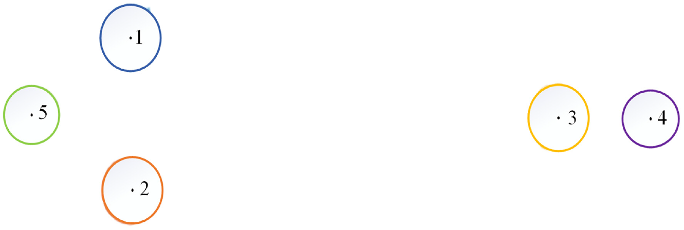
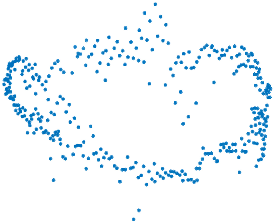
The smiley face point cloud model was used for verification. Set epsilon to 1 and Minpts to 4. The algorithm diagram is shown in Figure 2(a). As seen in Figure 2(b), the points with different results are marked with different colors, and those without colors are discrete points.

Figure 2.

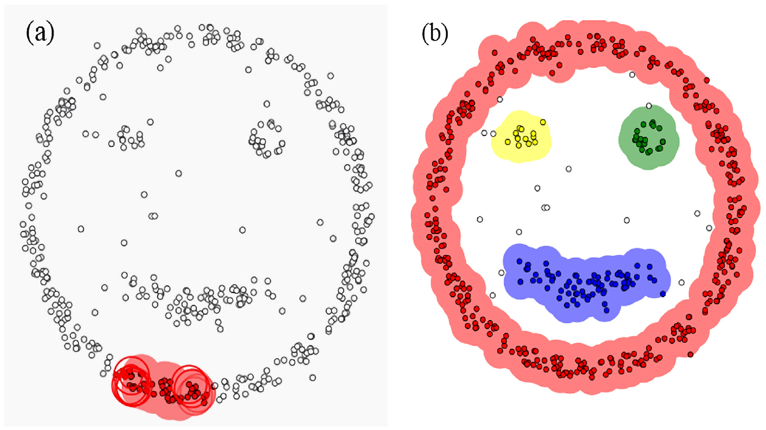
DBSCAN clustering algorithm: (a) schematic diagram of algorithm principle and (b) clustering results.

Point cloud circle feature recognition and extraction algorithm

Firstly, the maximum distance feature in the cluster is calculated after clustering. Secondly, the distribution function of maximum distance feature is optimized using nonparametric estimation and the feature histogram is established. The hole feature is extracted and the circular center position is calculated. Finally, the rationality of detecting circular hole features is determined by the degree of dispersion from the edge point to the center position.

Circle feature density histogram interval calculation

In this research, a maximum distance distribution technique based on nonparametric estimation²¹ is suggested to separate point cloud edge shape features and noise points for circular feature detection and extraction, taking into account the complicated porous structure.

After clustering the edge of point cloud E(q_i), the Cluster C = {C_l| C_l, l = 1,2,3,···, m} is produced, where p_i(C_l) is the coordinate of a point in C_l. Calculate the greatest point-to-point Euclidean distance in C_l using (4):

MaxD = max (| p_{i} (C_{l}) - p_{j} (C_{l}) |)

(4)

Continue to identify the two points with the greatest distance among the remaining points by storing p_i(C_l) and p_j(C_l) in sets A and B, respectively. f(A_i, B_i) → MaxD_i is the equivalent relationship between the points and the maximum distance. The diameter is the maximum point distance, and f(A_i, B_i) → MaxD_i may be used to locate the circular feature’s stable point.

To evaluate the degree of data density, the density histogram usually has to assume parameters.¹⁶ This work uses the probability density function to show the degree of sparseness of point cloud data and nonparametric function estimation to determine the interval of the probability density function to better identify feature points from nonfeature points.

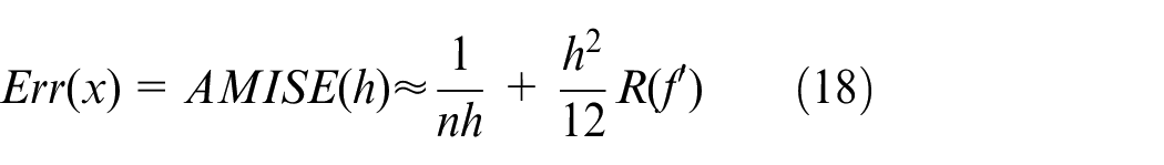
The error function Err(x) is defined as the optimization criterion for nonparametric estimation to make the fitted probability function more accurate, as demonstrated in (5):

Err (x) = E [{(y - \hat{f} (x))}^{2}]

(5)

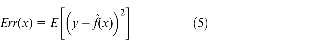
where y is the actual value, and $\hat{f} (x)$ is the fitting function. The degree of coincidence between the fitted function and the real function is represented by the error function Err(x), and y is represented by the actual parameter distribution function f(x) and error ε, as shown in (6):

y = f (x) + ε, ε ~ N (0, σ_{ε}^{2})

(6)

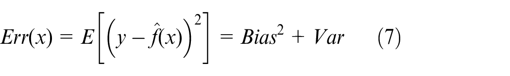
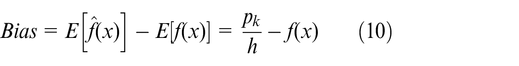
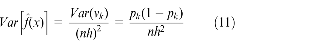
Err(x) is represented by the function deviation Bias and variance Var, where Bias is the discrepancy between the fitted function and the real function, and Var is the degree of dispersion of the fitted values since f(x) and ε cannot be calculated. As shown in (7):

Err (x) = E [{(y - \hat{f} (x))}^{2}] = Bia s^{2} + Var

(7)

After setting the optimization standard, estimate the density histogram with the nonparametric function to obtain the ideal interval width h*. The steps of the algorithm are as follows:

(1) First, as shown in Figure 3, the distance between two points in cluster C_l is computed and shown as a distance density histogram.

(2) The interval is set to B_k, interval width to h, probability function to v_k, and related probability density function to $\hat{f} (x)$ . The number of samples to calculate is set to n. Normalization reduces the sample data’s overall distribution probability to 1, as illustrated in (8):

\hat{f} (x) = \frac{v_{k}}{nh} = \frac{1}{nh} \sum_{i = 1}^{n} I_{B_{k}} (x_{i})

(8)

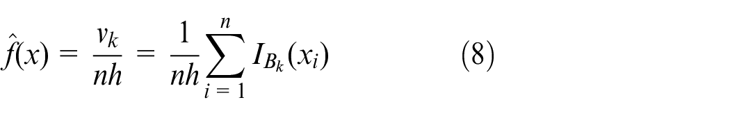
(3) Because each interval and distance data have a one-to-one relationship, the probability function v _k of the interval is assumed to conforms to the binomial distribution, as shown in equation (9):

v_{k} ~ B (n, p_{k}), where p_{k} = \int_{B_{k}} f (t) dt

(9)

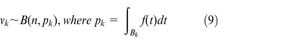
(4) The actual distance distribution function f(x) exists and is determined. Then, the expectation of f(x) is itself. Therefore, the expectation and variance of $\hat{f} (x)$ are as in (10) and (11):

Bias = E [\hat{f} (x)] - E [f (x)] = \frac{p_{k}}{h} - f (x)

(10)

Var [\hat{f} (x)] = \frac{Var (v_{k})}{{(nh)}^{2}} = \frac{p_{k} (1 - p_{k})}{n h^{2}}

(11)

(5) According to the median theorem shown in equation (12), the variance is integrated to calculate the IV (Integrated variance) of the fitting function, as shown in equation (13).

p_{k} = \int_{B_{k}} f (t) dt = hf (ξ) ξ \in B_{k}

(12)

\begin{matrix} IV = \int_{- \infty}^{+ \infty} Var [\hat{f} (x)] dx = \sum_{k = - \infty}^{+ \infty} \frac{p_{k} (1 - p_{k})}{nh} \\ = \frac{1}{nh} - \frac{R (f)}{n} R (f) = \int f {(x)}^{2} dx \end{matrix}

(13)

Figure 3.

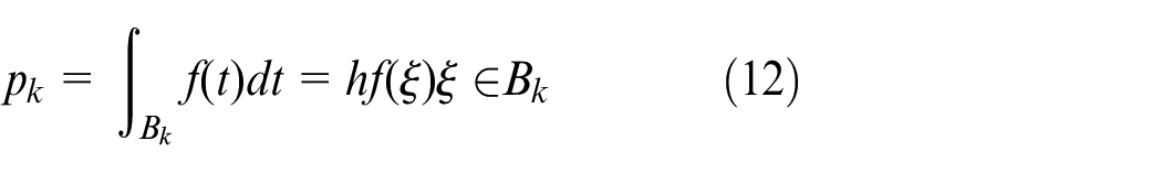
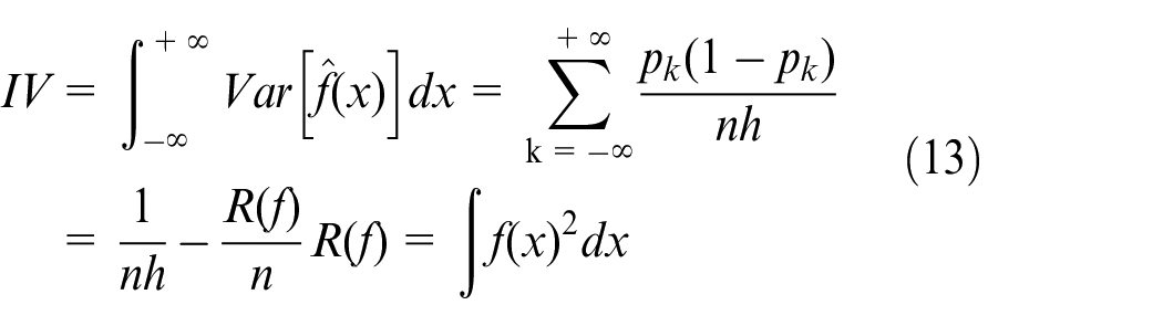
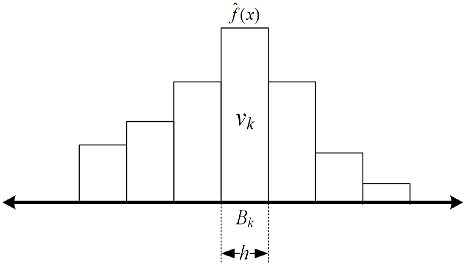
Diagram of density histogram.

According to Taylor series expansion formula (12), as follows:

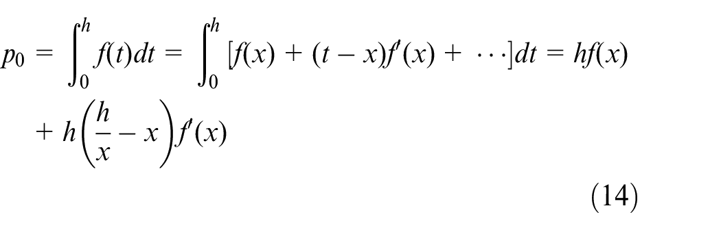
\begin{matrix} p_{0} = \int_{0}^{h} f (t) dt = \int_{0}^{h} [f (x) + (t - x) f' (x) + \dots] dt = hf (x) \\ + h (\frac{h}{x} - x) f' (x) \end{matrix}

(14)

Substituting into equation (10), as follows:

Bia s_{B_{0}} = (\frac{h}{2} - x) f' (x) + O (h^{3})

(15)

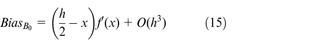
According to the generalized integral median theorem, it can be calculated as:

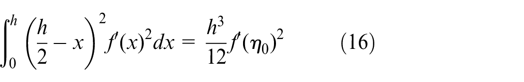
\int_{0}^{h} {(\frac{h}{2} - x)}^{2} f' {(x)}^{2} dx = \frac{h^{3}}{12} f' (η_{0})^{2}

(16)

Integrating the squared bias of equation (16) yields the ISB (Integrated squared bias) of the fitted function:

ISB = \frac{h^{2}}{12} \sum_{k = - \infty}^{+ \infty} hf' {(η_{k})}^{2} = \frac{h^{2}}{12} R (f') + o (h^{2})

(17)

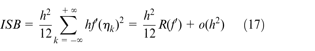
Calculate AMISE (Asymptotic mean integrated squared error) by combining formulas (13) and (17) into formula (7), and when Err(x) is the minimum, get the best solution h* of parameter h:

Err (x) = AMISE (h) \approx \frac{1}{nh} + \frac{h^{2}}{12} R (f')

(18)

h^{*} = {[\frac{6}{nR (f')}]}^{\frac{1}{3}}

(19)

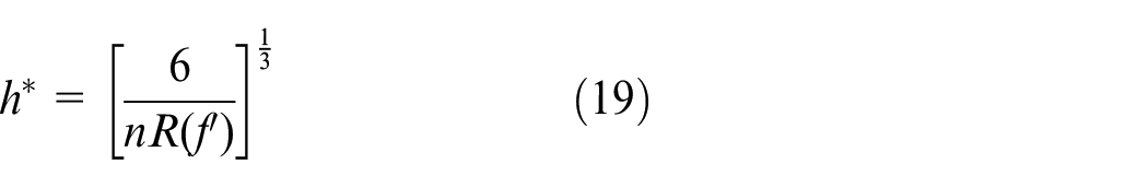
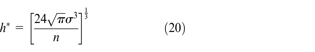
(6) The type of distance histogram distribution is determined. After analysis, the histogram of the distance between two points in cluster C_l is an approximately normal distribution. Then, f ∼ N(μ,σ²), where μ, σ are determined according to the actual distribution of the data, and the ideal interval h* is derived, as indicated in (12):

h^{*} = {[\frac{24 \sqrt{π} σ^{3}}{n}]}^{\frac{1}{3}}

(20)

Circle feature recognition and extraction

A maximum distance feature density histogram is created once the aforementioned approach is executed, as shown in Figure 4.

Figure 4.

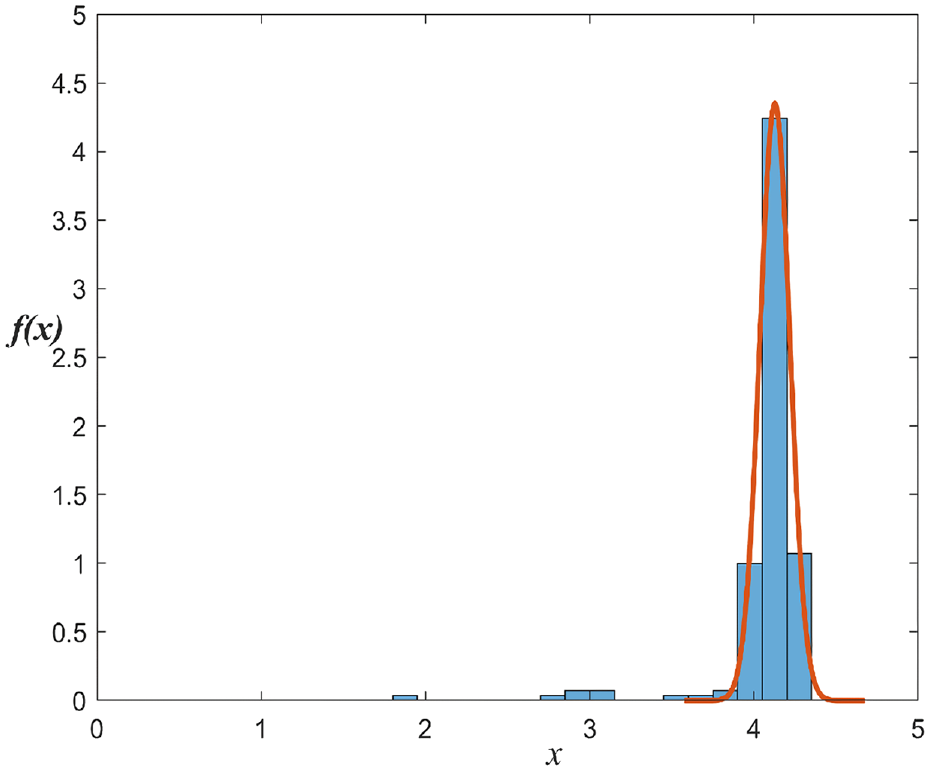
Distance feature histogram.

Set a threshold T based on the sparseness of feature points, extract feature points, and record the number n of feature points. The feature estimation has the most stability when T = 0.5, according to the experimental effect study. The cluster C_l’s center point O_l (x_l, y_l, z_l) is thus represented in (21):

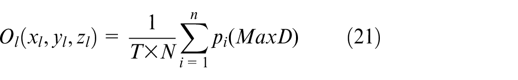
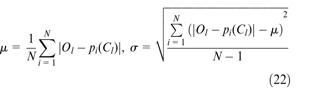
O_{l} (x_{l}, y_{l}, z_{l}) = \frac{1}{T \times N} \sum_{i = 1}^{n} p_{i} (MaxD)

(21)

Where N is The number of points in cluster C_l, and the extracted feature point is p_i (MaxD). This is determined if Cluster C_l is a 3D circular feature based on the discrete degree σ of the distance from each point in Cluster C_l to O_l (x_l, y_l, z_l).

As indicated in (22), the distance probability density histogram can be μ and σ.

μ = \frac{1}{N} \sum_{i = 1}^{N} | O_{l} - p_{i} (C_{l}) |, σ = \sqrt{\frac{{\sum_{i = 1}^{N} (| O_{l} - p_{i} (C_{l}) | - μ)}^{2}}{N - 1}}

(22)

Assuming that Cluster C_l is a circle feature, the radius r of the circle can be expressed by (24):

r = \frac{1}{n} \sum_{i = 1}^{n} | O_{l} - p_{i} (MaxD) |

(23)

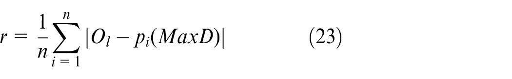
The judgment condition of whether it is a circle feature is shown in (24):

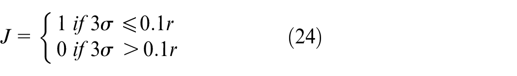
J = {\begin{matrix} 1 if 3 σ \leq 0.1 r \\ 0 if 3 σ > 0.1 r \end{matrix}

(24)

When J = 1, the cluster C_l is found to be a circular feature cluster by the formula. The feature points are those that fulfill the maximum distance interval h*.

Randomly select a point cloud cluster of a hole. Figure 5(a) is the effect diagram after denoising, edge point extraction and point cloud clustering. It can be seen that there are still many discrete points around the hole. Figure 5(b) shows the distribution of circular hole feature points extracted from the maximum distance feature density histogram optimized by nonparametric estimation. The distribution of red dots is relatively uniform. The result indicates that the feature points of circular hole can be accurately extracted and increase the accuracy of circular hole discrimination.

Figure 5.

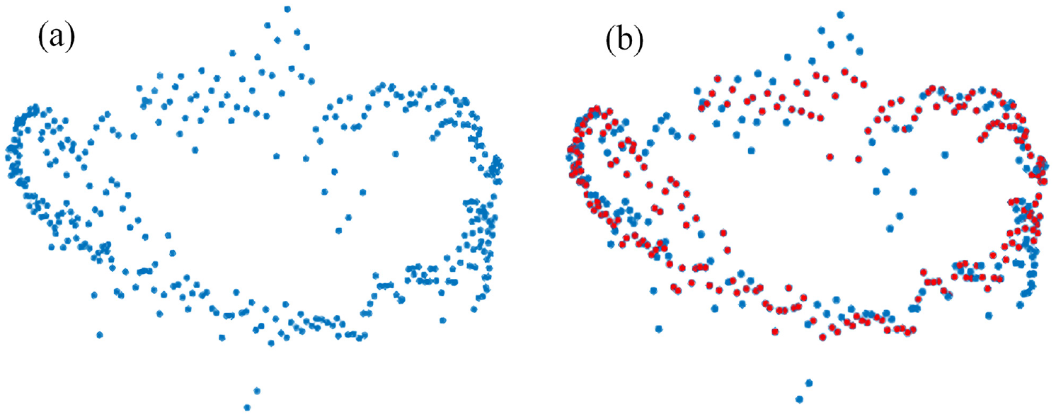
Distribution diagram of feature points: (a) feature points distribution and (b) optimized feature points distribution.

Comparison and analysis of tests

Construction of test platform

A binocular laser scanner, high-precision motion slide, liftable screw, motion motor control module, and optical precision damping vibration isolation platform comprise the 3D point cloud scanning detection system employed in this research, as shown in Figure 6. To realize overall workpiece scanning, a fixture is used to fix the grid assembly on the placing table, the height of the z-axis is set, the x-axis is scanned repeatedly with the dual-line laser scanner, and the y-axis of the placing table is quantitatively moved. The entire scanning system is fixed on an optical precision damping vibration isolation platform to reduce the influence of the slight ground vibration on the scanning results.

Figure 6.

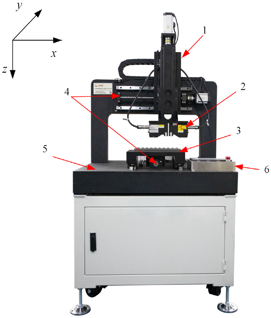
3D point cloud scanning detection system. 1 – Lifting screw. 2 – Binocular laser scanner. 3 – Workpiece placement table to be tested. 4 – High-precision motion slide. 5 – Optical precision damping vibration isolation platform. 6 – Sports console.

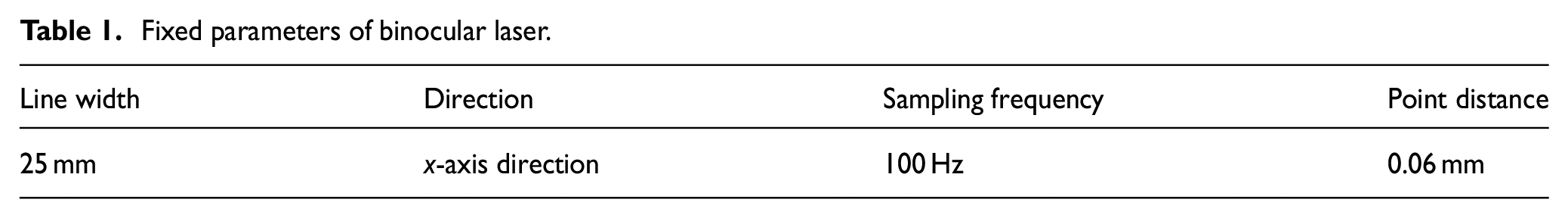
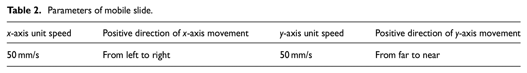
Tables 1 and 2 illustrate the speed of the sliding table, positive direction of movement, movement distance, and fixed parameters of the line laser.

Table 1.

Fixed parameters of binocular laser.

Line width	Direction	Sampling frequency	Point distance
25 mm	x-axis direction	100 Hz	0.06 mm

Table 2.

Parameters of mobile slide.

x-axis unit speed	Positive direction of x-axis movement	y-axis unit speed	Positive direction of y-axis movement
50 mm/s	From left to right	50 mm/s	From far to near

Point cloud model

The surface depth information of the part is measured using double line laser sensor. The 3D coordinates of each point on the workpiece surface can be obtained through the registration of the slide encoder information of x-axis, y-axis. The point cloud dataset of the parts is constructed by registration and splicing, and 3D reconstruction is completed. The scanning scheme of point cloud model is as follows:

(1) Completely scan the analyte in the positive x -axis direction and then shift it to the positive y -axis direction each time l : l is the line laser’s line width. Scanning the analyte along the x -axis should be repeated until scanning is complete;

(2) Calculate the coordinates of all scanned data points using the high-precision sliding table coordinate system, filter out any redundant points that have no information, and acquire coordinate information for all points;

(3) The z -axis direction remains constant during the scanning procedure. The registration and splicing of point clouds is accomplished by using the same coordinate superposition in the y -axis direction.

Test design

A comparative experiment of 3D circle feature extraction is planned to validate the 3D circle feature recognition and extraction technique proposed in this paper. First, the edge of the point cloud is extracted for the point cloud model of grid assembly and plane rectangular flange. Second, a circular hole was randomly selected, a density histogram was constructed using different interval widths, and the feature probability density function was fitted to verify the influence of the density histogram interval width h on the feature extraction accuracy and to prove the necessity of nonparametric estimation optimization. And last, the extracted circle features are tested and compared using the traditional circle feature recognition technique (the Least Squares and Random Sampling Consensus (RANSAC)²²) and the algorithm presented in this research.

Result analysis

Figure 7(a) shows the point cloud model of grid assembly, which has a total of 1,981,594 points. Figure 7(b) shows the related edge point cloud model, which has a total of 125,785 points after edge extraction.

Figure 7.

Grid assembly point cloud model edge extraction renderings: (a) before edge extraction and (b) after edge extraction.

The edge points are clustered to obtain 102 hole categories, as shown in Figure 8:

Figure 8.

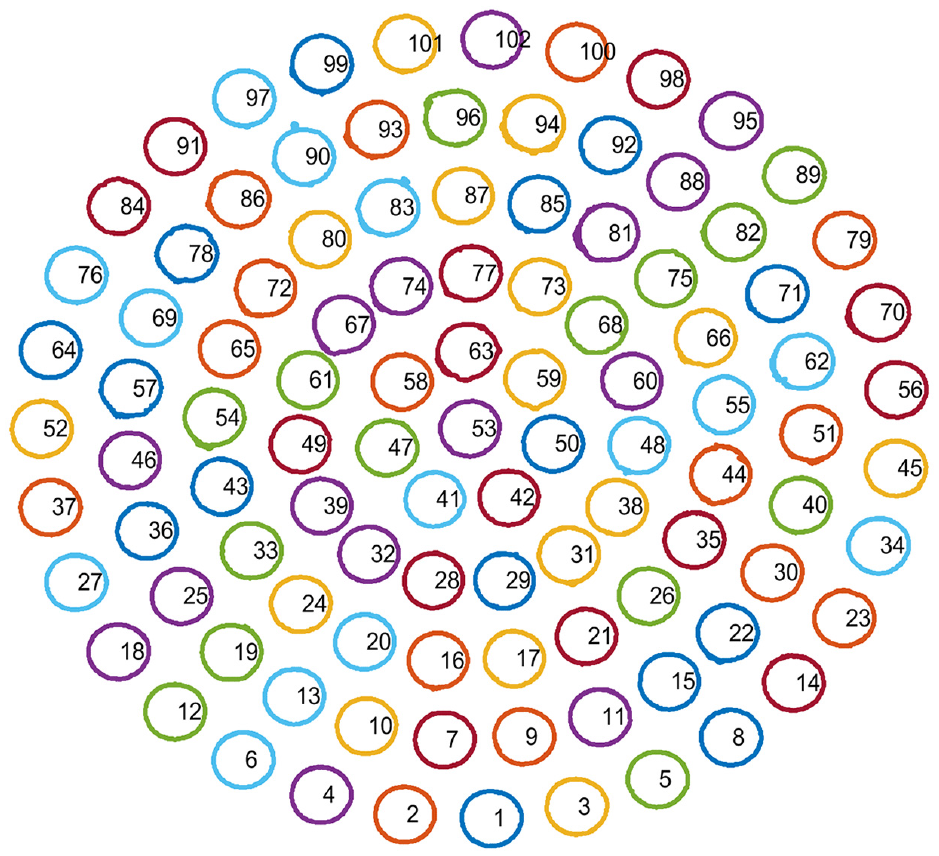
Renderings of hole clustering of grid assembly.

The other piece to be tested is a rectangular flange, with a total of 1,017,564 points in the point cloud model. By using a distance density based edge point extraction algorithm, a total of 12,800 points were extracted for subsequent calculations after denoising, as shown in Figure 9.

Figure 9.

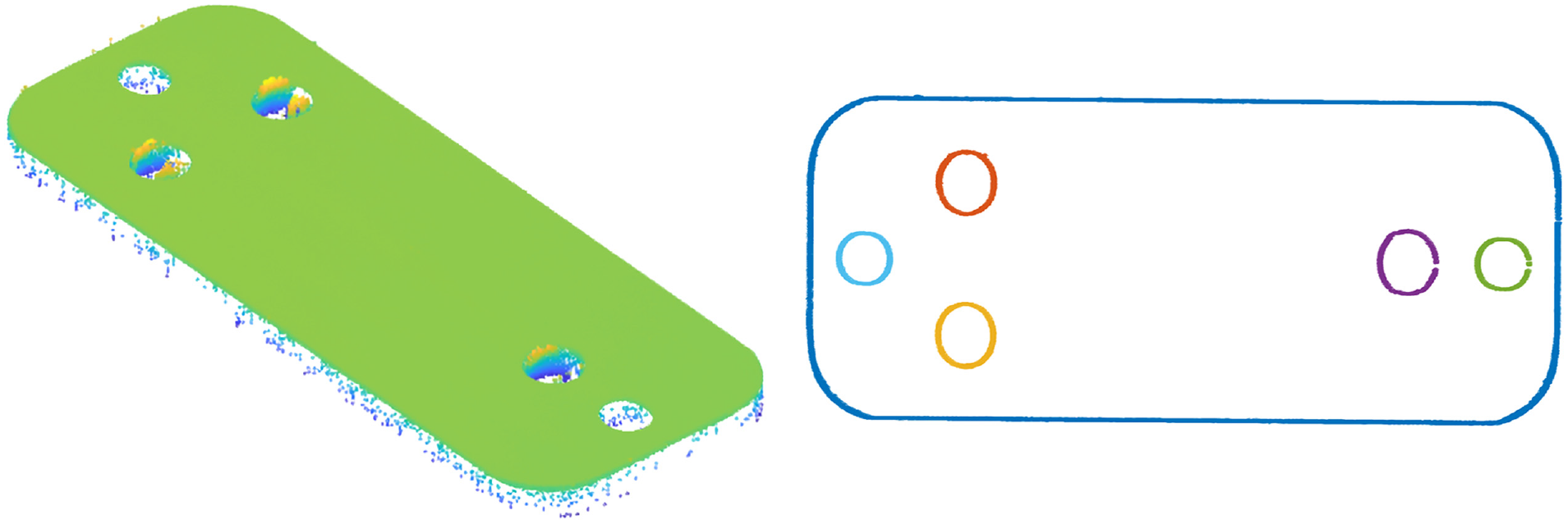
Plane flange point cloud model and edge extraction.

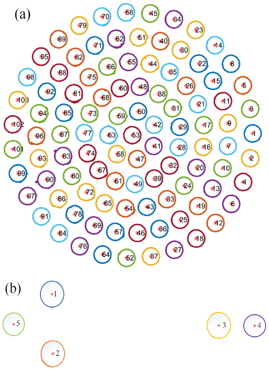
The edge points are clustered to obtain five hole categories, as shown in Figure 10.

Figure 10.

Renderings of hole clustering of rectangular flange.

Randomly select a cluster as shown in Figure 11, the ideal histogram interval h* is 0.15 mm according to formula (21). And AMISE calculates Err(x) using formula (19). Calculate the density function error and create a density histogram for data comparison analysis using the interval widths h = 0.01, h = 0.3, and h = 0.6 mm, respectively. As shown in Figure 12(a)–(d), the AMISE of the corresponding characteristic density functions of h* = 0.15, h = 0.01, and h = 0.3 mm, and h = 0.6 mm are 0.0491, 0.5348, 0.0729, and 0.2292 mm².

Figure 11.

Randomly extracting round hole clusters.

Figure 12.

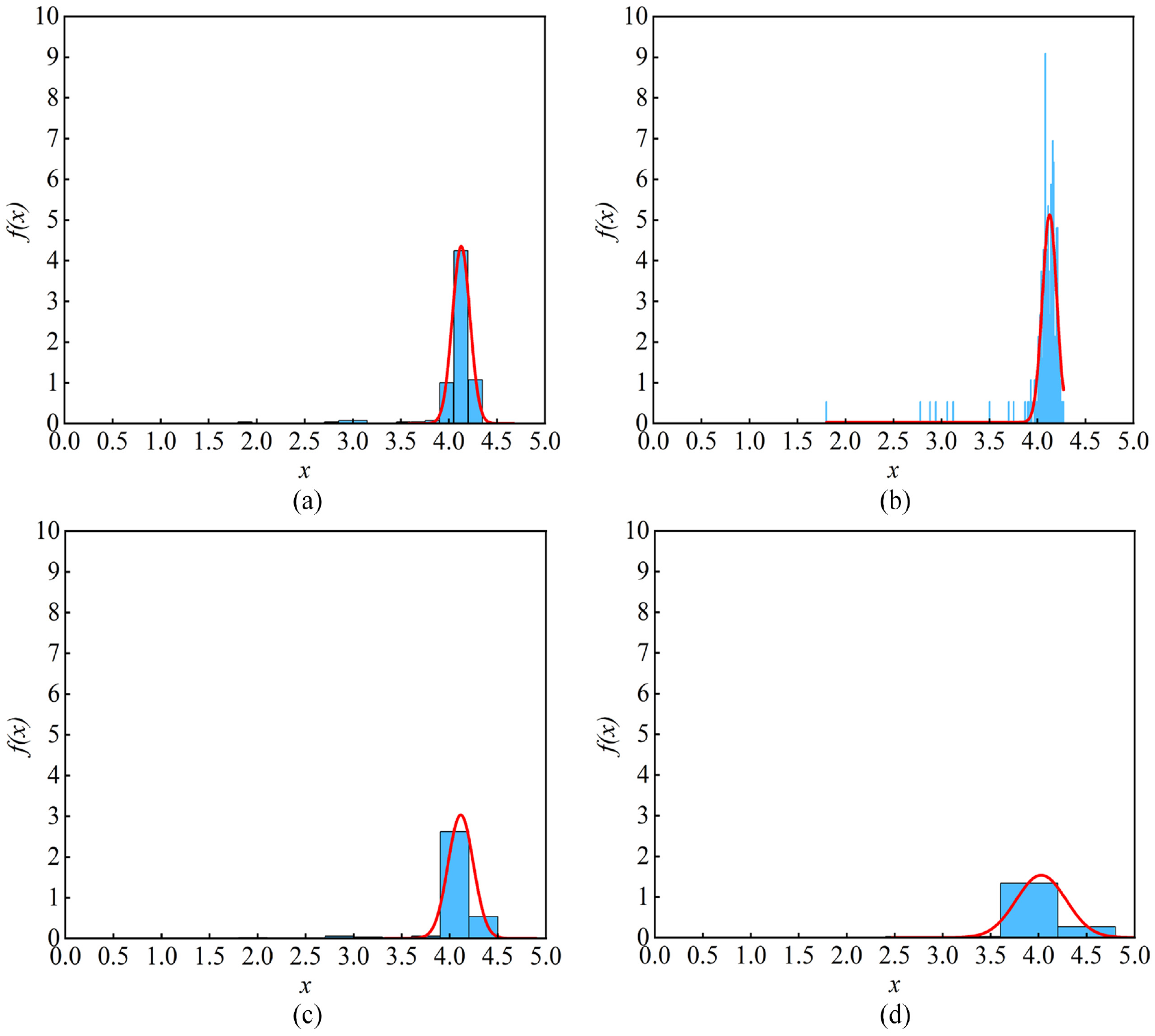
Nonparametric estimation optimization comparison: (a) h* = 0.15, AMISE = 0.0491, (b) h = 0.01, AMISE = 0.5348, (c) h = 0.3, AMISE = 0.0729, and (d) h = 0.6, AMISE = 0.2292.

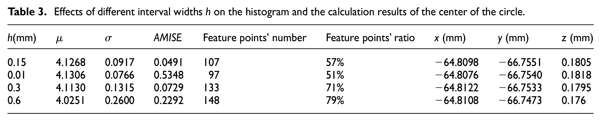
The error Err(x) of the feature probability density function under nonparametric estimation is smaller in AMISE, and the greater the distance h* = 0.15 mm, the larger the Err(x). It can be shown that the density histogram’s interval width h has an impact on the probability density function’s correctness, which in turn has an impact on feature point selection. There are 187 random circular holes in total, with the fraction of extracted feature points falling within the P (0.25 < X < 0.75) probability interval. The probability of noise in the retrieved feature points changes as the interval width h increases, as shown in Table 3. If it is large, the fraction of feature points exceeds the probability interval P, resulting in a larger function deviation and affecting the center of the circle calculation accuracy. The genuine circle center should be near h = 0.3 and h* = 0.15, according to the data in Figure 12 and the change trend of the circle center coordinates in Table 3. The z-axis coordinate data displays a declining trend due to the growing proportion of noise points involved in the calculation between the point cloud layers.

Table 3.

Effects of different interval widths h on the histogram and the calculation results of the center of the circle.

h(mm)	μ	σ	AMISE	Feature points’ number	Feature points’ ratio	x (mm)	y (mm)	z (mm)
0.15	4.1268	0.0917	0.0491	107	57%	−64.8098	−66.7551	0.1805
0.01	4.1306	0.0766	0.5348	97	51%	−64.8076	−66.7540	0.1818
0.3	4.1130	0.1315	0.0729	133	71%	−64.8122	−66.7533	0.1795
0.6	4.0251	0.2600	0.2292	148	79%	−64.8108	−66.7473	0.176

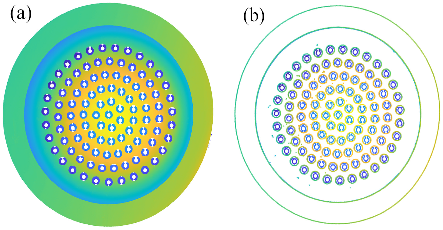
The choice of the interval width of the density histogram is particularly crucial to the accuracy of fitting the probability density function. A nonparametric estimation method is used to obtain the ideal interval width h*, which reduced function fitting error and improved the accuracy of 3D circular feature extraction. The circular hole recognition results of the point cloud model are plotted in Figure 13, including grid assembly and plane flanges.

Figure 13.

The circular hole recognition results: (a) grid assembly and (b) plane flanges.

The Least Square method, RANSAC algorithm and the algorithm proposed in the paper are used for algorithm comparison test, and the results are depicted in Figure 14. Figure 14(a) and (d) demonstrate the fitting effect and position of the center of a circle in 3D space using the Least Square method. In the case of uneven edge density distribution, there are significant errors in circle fitting and center calculation. Using RANSAC algorithm, the fitting effect and position of the circle center are shown in Figure 14(b) and (e). It can be seen that due to the structure of the circular hole on the arch surface, the normal vector has a large deviation between the fitting circle and the actual circle, resulting in inaccurate identification. The proposed algorithm is used for processing. The optimal maximum distance interval is selected through nonparametric estimation. The optimal circle feature points are extracted and the center of the circle is calculated, as illustrated in Figure 14(c) and (f). The discrete degree of the distance from the edge point to the center by the three methods is 1.3354, 0.3925, and 0.0417, respectively. The precision of center coordinates obtained by this method is obviously better than that of the Least Square method and RANSAC algorithm, and 3D circular hole feature can be accurately identified and extracted. Compared with the Least Square method and RANSAC algorithm, the method can reduce the noise of edge data, so as to obtain better feature extraction effect. Therefore, the proposed algorithm in this paper has better accuracy in the case of uneven distribution of point clouds and noise points in practical applications.

Figure 14.

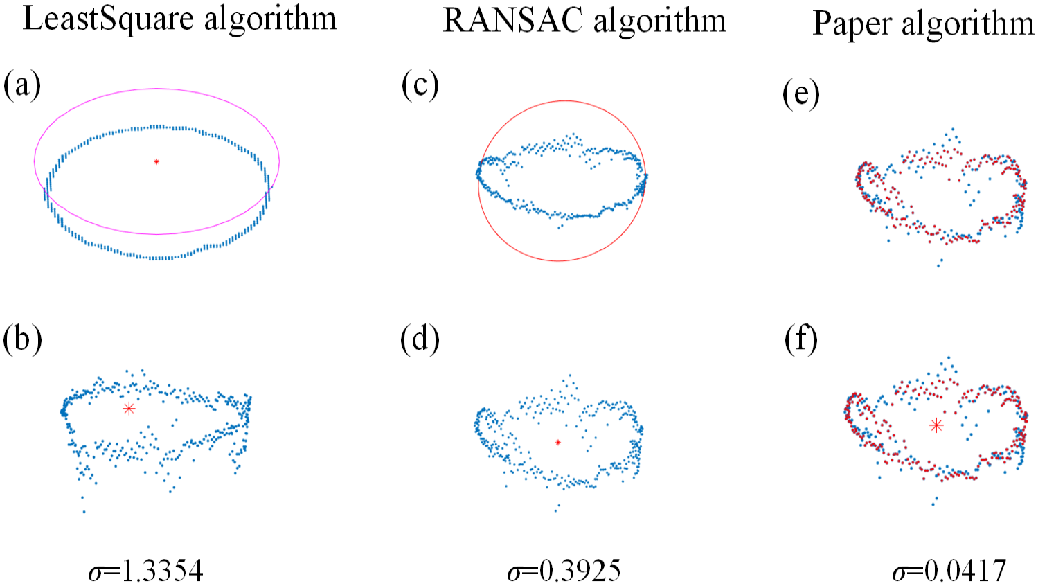
Comparison of circle feature recognition results: (a and d) circle fitted by Least Square method and display of calculated circle center in 3D space, (b and e) circle fitted by RANSAC algorithm and calculated center of circle are displayed in 3D space, and (c and f) circle feature points extracted by paper algorithm and display of calculated circle center in 3D space.

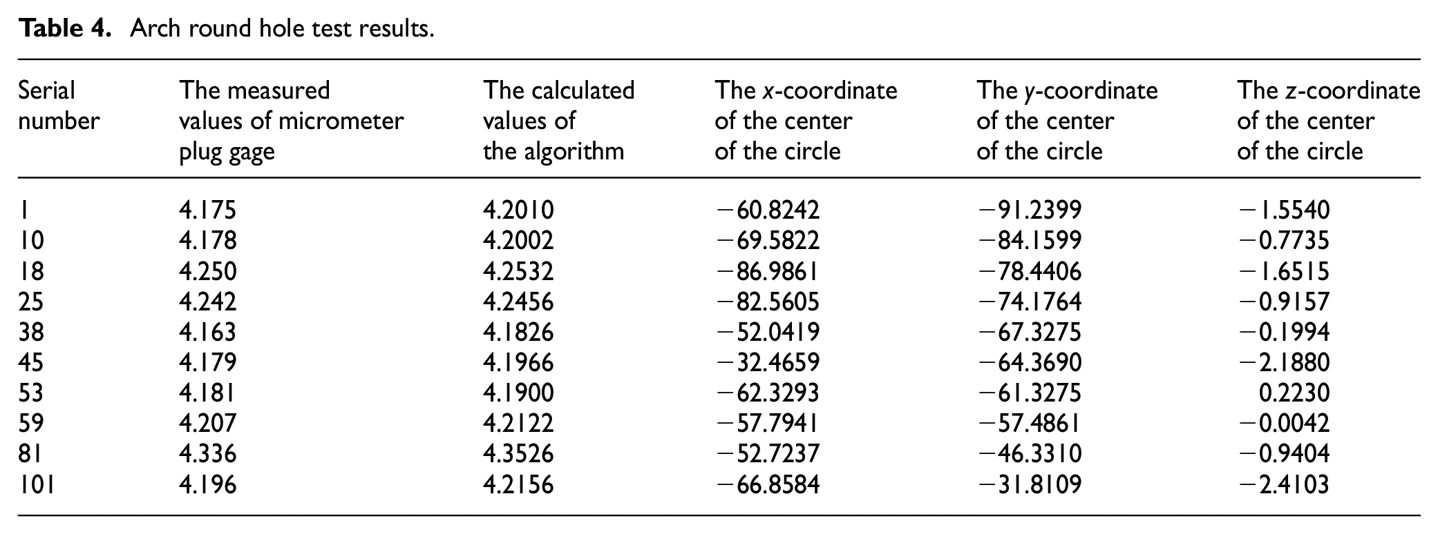
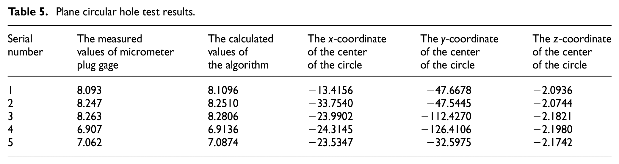
Finally, the accuracy of the algorithm is verified by comparing with the measured value of micrometer plug gage. Several groups of data are randomly selected to test the diameter measurement error. The results are shown in Tables 4 and 5. The measured values of micrometer plug gage and the calculated values of the algorithm in this paper are given in the tables. The last three columns of data are the xyz coordinates of the circle center by the algorithm. Compared with the measured value of the plug gage, the average measurement error of arch round hole of the algorithm in this paper is 11.5 μm, the maximum measurement error is 26 μm, and the standard deviation is 8.1 μm. The average measurement error of plane circular hole is 11.4 μm, the maximum measurement error is 25.6 μm, and the standard deviation is 7.8 μm. The results show that the proposed algorithm is suitable for both arch and plane circular holes, and it has high precision.

Table 4.

Arch round hole test results.

Serial number	The measured values of micrometer plug gage	The calculated values of the algorithm	The x-coordinate of the center of the circle	The y-coordinate of the center of the circle	The z-coordinate of the center of the circle
1	4.175	4.2010	−60.8242	−91.2399	−1.5540
10	4.178	4.2002	−69.5822	−84.1599	−0.7735
18	4.250	4.2532	−86.9861	−78.4406	−1.6515
25	4.242	4.2456	−82.5605	−74.1764	−0.9157
38	4.163	4.1826	−52.0419	−67.3275	−0.1994
45	4.179	4.1966	−32.4659	−64.3690	−2.1880
53	4.181	4.1900	−62.3293	−61.3275	0.2230
59	4.207	4.2122	−57.7941	−57.4861	−0.0042
81	4.336	4.3526	−52.7237	−46.3310	−0.9404
101	4.196	4.2156	−66.8584	−31.8109	−2.4103

Table 5.

Plane circular hole test results.

Serial number	The measured values of micrometer plug gage	The calculated values of the algorithm	The x-coordinate of the center of the circle	The y-coordinate of the center of the circle	The z-coordinate of the center of the circle
1	8.093	8.1096	−13.4156	−47.6678	−2.0936
2	8.247	8.2510	−33.7540	−47.5445	−2.0744
3	8.263	8.2806	−23.9902	−112.4270	−2.1821
4	6.907	6.9136	−24.3145	−126.4106	−2.1980
5	7.062	7.0874	−23.5347	−32.5975	−2.1742

Conclusion

Using nonparametric estimation methods, the paper proposes an algorithm for 3D round hole feature detection based on point cloud feature extraction. The algorithm effectively avoids the calculation deviation caused by traditional algorithm circle fitting. It can be seen from Figure 14 that compared with the Least Squares method and RANSAC algorithm, the center coordinates obtained by this algorithm are more accurate and the extraction of edge data is more effective. Thus, the precision of 3D circular hole feature extraction is improved.

By building an experimental testing platform, algorithm testing was conducted on the grid assembly device printed parts (arch round hole) and rectangular flange (plane round hole). The average error of the diameter detection results of the circular hole on the arch surface is 11.5 μm. The standard deviation is 8.1 μm. The average error of the diameter of flat circular hole is 11.4 μm. The standard deviation is 7.8 μm. The results indicate that the proposed algorithm can effectively extract 3D circular hole features from point clouds with dispersed circular holes on arch surfaces and planar surfaces. The research results are expected to provide a certain theoretical basis and technical support for automatic detection of 3D circular hole feature extraction.

Footnotes

Declaration of conflicting interests

The author(s) declared no potential conflicts of interest with respect to the research, authorship, and/or publication of this article.

Funding

The author(s) disclosed receipt of the following financial support for the research, authorship, and/or publication of this article: The authors would like to acknowledge financial support provided by the Scientific and Technological Project of Songjiang District in Shanghai (20SJKJGG08C) and Jiangsu Provincial Engineering Research Center of Robot and Intelligent Manufacturing Equipment Open Subject (SDGC2254).

ORCID iDs

Hao Yang

Haoyu Li

Data availability statement

Data sharing not applicable to this article as no datasets were generated or analyzed during the current study.

References

Watson

EA.

Viewpoint-independent object recognition using reduced-dimension point cloud data. J Opt Soc Am A 2021; 38(10): B1–B9.

Yeom

Javidi

Three-dimensional object feature extraction and classification with computational holographic imaging. Appl Opt 2004; 43(2): 442–451.

Gai

Zeng

, et al. Research on a hole filling algorithm of a point cloud based on structure from motion. J Opt Soc Am A 2019; 36(2): A39–A46.

Belmekki

MAA

Tobin

Buller

, et al. Fast task-based adaptive sampling for 3D single-photon multispectral lidar Data. IEEE Trans Comput Imaging 2022; 8: 174–187.

Feng

Gao

, et al. 3D reconstruction of structured light fields based on point cloud adaptive repair for highly reflective surfaces. Appl Opt 2021; 60(24): 7086–7093.

Wakayama

Takahashi

Ono

, et al. Three-dimensional measurement of an inner surface profile using a supercontinuum beam. Appl Opt 2018; 57(19): 5371–5379.

Wei

Huang

Xie

, et al. Mesh denoising guided by patch normal co-filtering via kernel low-rank recovery. IEEE T Vis Comput Gr 2019; 25(10): 2910–2926.

Hashimoto

Saito

. Normal estimation for accurate 3D mesh reconstruction with point cloud model incorporating spatial structure. In: IEEE CVPR, Los Alamitos, USA, June 2019, pp.54–63. IEEE Computer Society Press.

Shi

Wang

Feature line extraction for point cloud based on normal vector region clustering segmentation. China Mech Eng 2021; 32(21): 2552–2561.

10.

Xue

Shen

, et al. Identification method for machine workpiece based on laser 3D point cloud. Infrared Laser Eng 2019; 48(4): 169–176.

11.

Demarsin

Vanderstraeten

Volodine

, et al. Detection of closed sharp edges in point clouds using normal estimation and graph theory. Comput Aided Des 2007; 39(4): 276–283.

12.

Wang

Chen

, et al. Feature line extraction from a point cloud based on region clustering segmentation. Acta Opt Sin 2018; 38(11): 66–75.

13.

Wang

Fan

, et al. Adaptive point cloud reduction based on multi parameter k-means clustering. Laser Optoelectron Prog 2021; 58(6): 175–183.

14.

Tabib

Jadhav

Tegginkeri

, et al. Learning-based hole detection in 3D point cloud towards hole filling. Procedia Comput Sci 2020; 171: 475–482.

15.

, et al. PointNet: deep learning on point sets for 3D classification and segmentation. In: IEEE CVPR, Los Alamitos, USA, 2017, pp.652–660. IEEE Computer Society Press.

16.

Wang

Ewert

Schilberg

, et al. Edge extraction by merging 3D point cloud and 2D image data. In: IEEE CEWIT, New York, NY, USA, 21–22 October 2013, pp.21–22. IEEE Computer Society Press.

17.

Bazazian

Casas

Ruiz-Hidalgo

Fast and robust edge extraction in unorganized point clouds. In: 2015 DICTA, Adelaide, Australia, 23–25 November 2015, pp.1–8. IEEE Computer Society Press.

18.

Zhang

Guo

, et al. KDD: a kernel density based descriptor for 3D point clouds. Pattern Recognit 2021; 111: 107691.

19.

Sun

, et al. A method for detecting high-frequency oscillations using semi-supervised K-means and mean shift clustering. Neurocomputing 2019; 350: 102–107.

20.

Kiyasu

Hoshino

Yano

, et al. Measurement of the 3-D shape of specular polyhedrons using an m-array coded light source. IEEE Trans Instrum Meas 1995; 44(3): 775–778.

21.

Scott

(ed.). Multivariate density estimation: theory, practice, and visualization. 2nd ed. New York, NY: John Wiley & Sons, 2015, p.425.

22.

Derpanis

KG.

Overview of the RANSAC algorithm. Image Rochester NY 2010; 4(1): 2–3.

Point cloud-based 3D round hole detection

Abstract

Keywords

Introduction

Point cloud model preprocessing algorithm

Establishment of topological relationships

Extraction of point cloud edges

Calculate the density of a point cloud

Set the distance threshold

Extraction of point cloud edges

Update the threshold coefficient

Cluster analysis of point clouds

Point cloud circle feature recognition and extraction algorithm

Circle feature density histogram interval calculation

Circle feature recognition and extraction

Comparison and analysis of tests

Construction of test platform

Point cloud model

Test design

Result analysis

Conclusion

Footnotes

Declaration of conflicting interests

Funding

ORCID iDs

Data availability statement

References