
Abstract
Metal magnetic memory (MMM) technique can detect macroscopic defects and stress concentration zones of ferromagnets, and it can identify the approximate positions of these flaws, while a little further information about defects characteristics can be provided. To promote study in this area, defects were modeled as located magnetic dipoles whose strength and locations should be determined, and the technique of truncated generalized inverse and reduced space inversion were used to image the dipole strength. Through the simulation experiment, we found that the inversion image quality was influenced by the lift-off value. When the magnetic field data for inversion was measured with a small lift-off value, the inner dipoles contributions were easily buried and the inversion image can only shown the surface dipole well. In contrast, if the magnetic field data was measured with a greater lift-off value, it was possible to inverse the deep dipoles while the image was somewhat out of focus. To overcome this limitation, we composed the magnetic field data measured under different lift-off values together for inversion. We used the same model to test this approach and applied it on real crack defects magnetic field data. It demonstrates that the new inversion approach shows better accuracy than the single lift-off value and it was possible to infer the location and size of defect by the evaluation of preset dipoles.
Introduction
Many engineering components and structures in service are working under circumstances of high temperatures, high speed and surrounding corrosion. It is necessary and important to conduct non-destructive inspections or monitor corrosion, cracks and other defects to ensure safety. However, the traditional non-destructive test (NDT) techniques, such as linear ultrasonic testing (UT), eddy current testing (ET), and magnetic flux leakage testing (MT) can only detect already developed defects.1–3 The metal magnetic memory (MMM) technique, proposed by Russian experts in the late 1990s, can find not only macroscopic defects, but also stress concentration zones and early damages.4,5 MMM technique has many advantages such as pre-processing free, rapid detection and easy operation, etc. Now it has become an emerging field in Russia and China.6–8
MMM is a non-destructive test method based on analysis of the self-magnetic leaked field (SMLF) above the surface of a component. 3 Because the physicality of MMM is unclear so far, many researchers have devoted their efforts to investigating regular variations of signals in the laboratory.4,7 Previous research studies on the MMM method have concentrated on the variation of signals under tensile stresses, cyclic tensile-compressive stress, and magneto mechanical effect.9–11 Although many experiments have been performed and many important achievements about the relationship between the SMLF and applied stress have been made, existing MMM technology is normally used to find the possible locations of defects, and assess the corrosion status of these critical components in cable-stayed bridges and other structures, but little further information about defect characteristics (e.g. defect depth and shape) can be provide. 2 The reason is that SMLF signal measured by the sensor is sensitive to a variety test parameters such as material permeability, stress, remanent magnetization, etc.12,13 This paper aims to present some analysis about the defect characteristics through determining the location and the strength of the dipoles that represent the defect from the SMLF signal measured above the sample surface. This advancement not only provides a more comprehensive understanding of defect characteristics but also facilitates the decision-making process for engineering test personnel.
Principle
Mathmatial of model
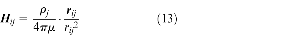
Magnetic dipole is a simple but applied broadly magnetic model. With characteristics of a different physical meaning and a clear geometric image, the magnetic dipole theory can be used to solve some theoretical problems in the magnetic detecting field. The magnetic flux leakage at scanning point p with coordinates (x i , y i ) produced by an individual magnetic dipole q j located at point (x j , y j ), as shown in Figure 1, can be obtained by the following equations14,15:
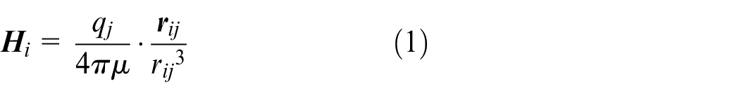
where r and r is the vector and distance from the magnetic dipole to the scanning point respectively, and μ is the magnetic permeability of air.
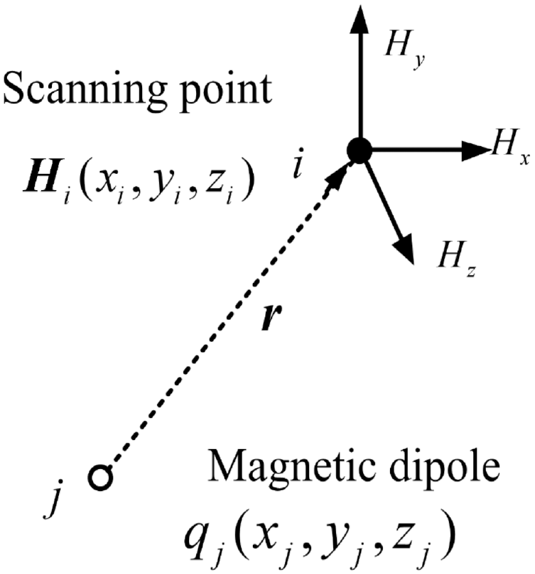
Magnetic field at a scanning points i induced by a magnetic.
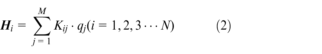
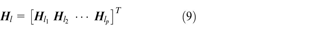
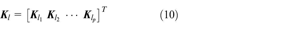
The area with defects can be divided into some elements for analysis. Assumed that the number of elements is M and the intensity of the leakage field was measured in N scanning points, the magnetic flux leakage H i at the scanning point i can be expressed by a linear combination of the magnetic flux leakage produced by individual magnetic dipoles as follows:
where
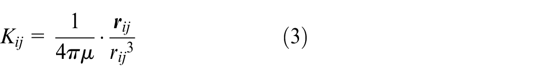
Equation (2) indicate that the magnetic flux leakage at scanning point i are given by the product of the strength of magnetic dipole q j located at a point j and the coefficient K ij respectively. 17 Since all data of magnetic flux leakage can be expressed as a column vector and similarly for the magnetic dipoles, the equation (2) can be rewritten in matrix form as:

where
When the data matrix

where

where
Truncated generalized inverse and reduced space inversion
In the Section II.A, we introduced the simple process for crack death determination. In general, the coefficient matrix
In the presence of noise, some of singular values reach very small and the full-rank inverse does not necessarily give good results. Hence, Bruno
16
present a method based on truncated generalized inverse to estimate the dipole strength, which the singular values less than a threshold are truncated and the truncated generalized inverse

To improve the results accuracy, Baskaran, et al, taken the first inversion results
Numerical simulation and results
As shown in Figure 2, a 10 mm × 10 mm rectangular bar is taken as the test specimen, and two line defects are considered as example. The defects located at x = −3 and 3 mm with y ranging from −1 to −2 mm and −1 to −6 mm respectively.
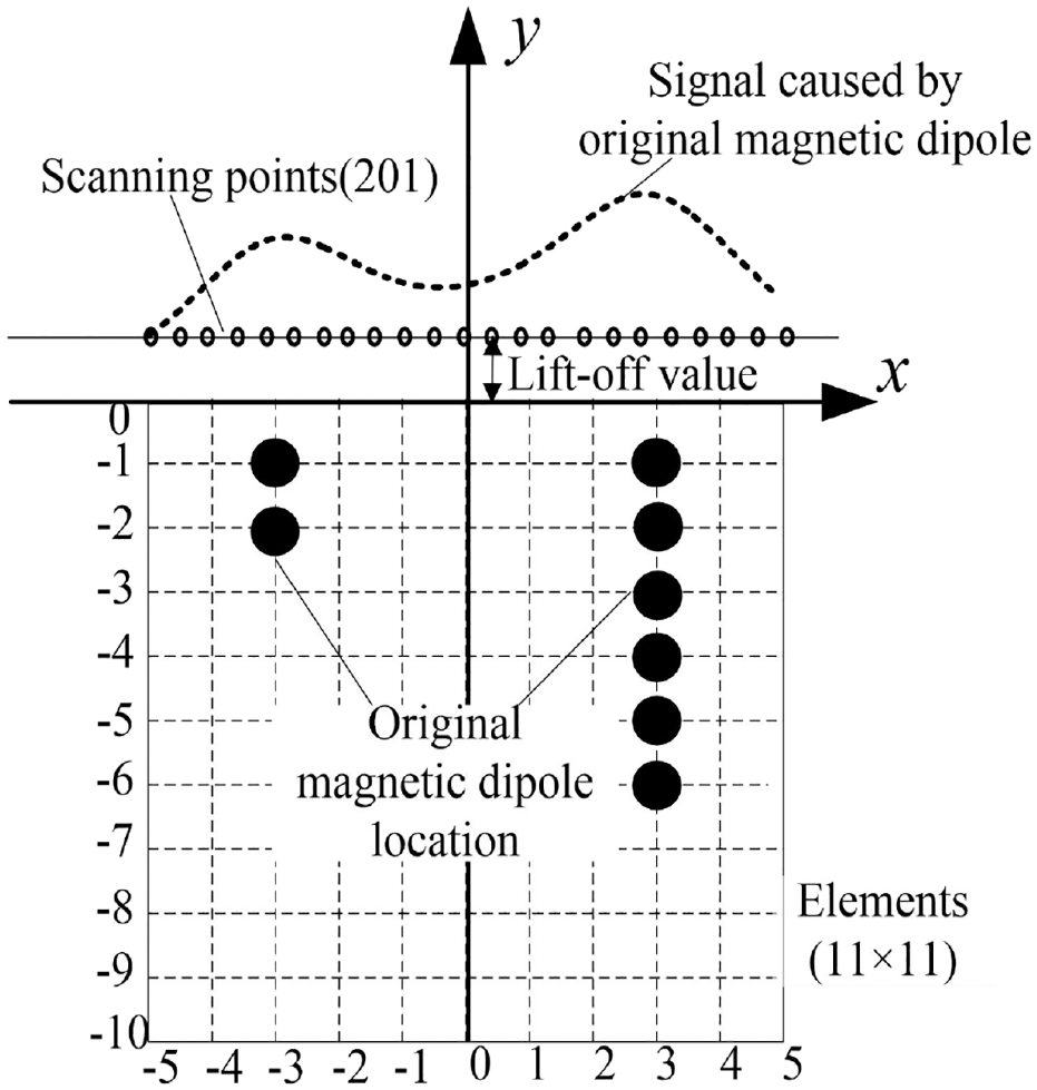
Schematic representation of the defect model.
For the convenience of discussion, the cross section of specimen is divided into 11 × 11 (121) locations in steps of 1.0 mm, and only on these locations, where there are defects q j s are taken to be finite and the rest of the locations are taken to be zeros. All the dipoles have the same strength and the image representation of the dipoles strength are shown in Figure 3. About 201 scanning points for measuring magnetic flux leakage are designed at certain intervals 0.05 mm on a line above the specimen with the lift-off value are 0.5, 1.0, and 3.0 mm respectively.
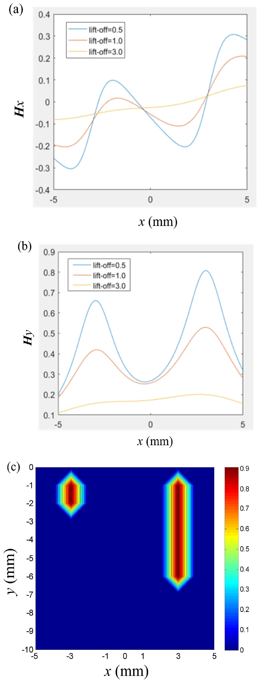
Magnetic field calculated by the dipole model at different lift-offs and image representation of defect dipole strength: (a) magnetic field component of x-direction, (b) magnetic field component of y-direction, and (c) image representation of defect dipole strength.
The coefficient matrix
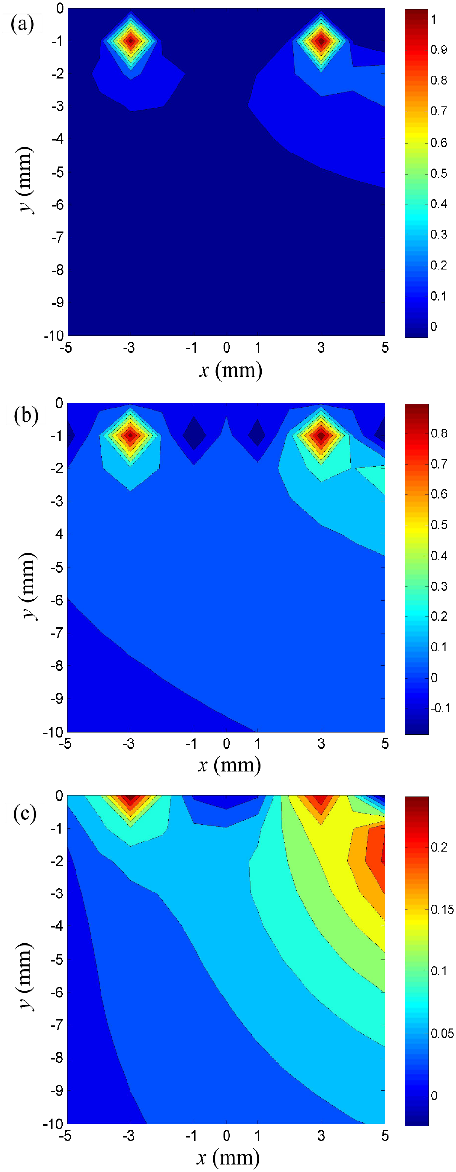
Image representation of recovery dipoles strength with the magnetic fields data for inversion were measured under a single lift-off value: (a) the lift-off value l is 0.5 mm, (b) l = 1.0 mm, and (c) l = 3.0 mm.
The first inversion result provide the dipole strength at all preset positions and the computed data of dipole strength scattered at the actual and nearby locations because of the finiteness and error of the measured data. To improve the inverted image quality, the minimum threshold of the maximum recovered dipole strength is used to select the specific location where the possibility of the defect exists. When the lift-off value are 0.5, 1.0, and 3.0 mm, the minimum threshold
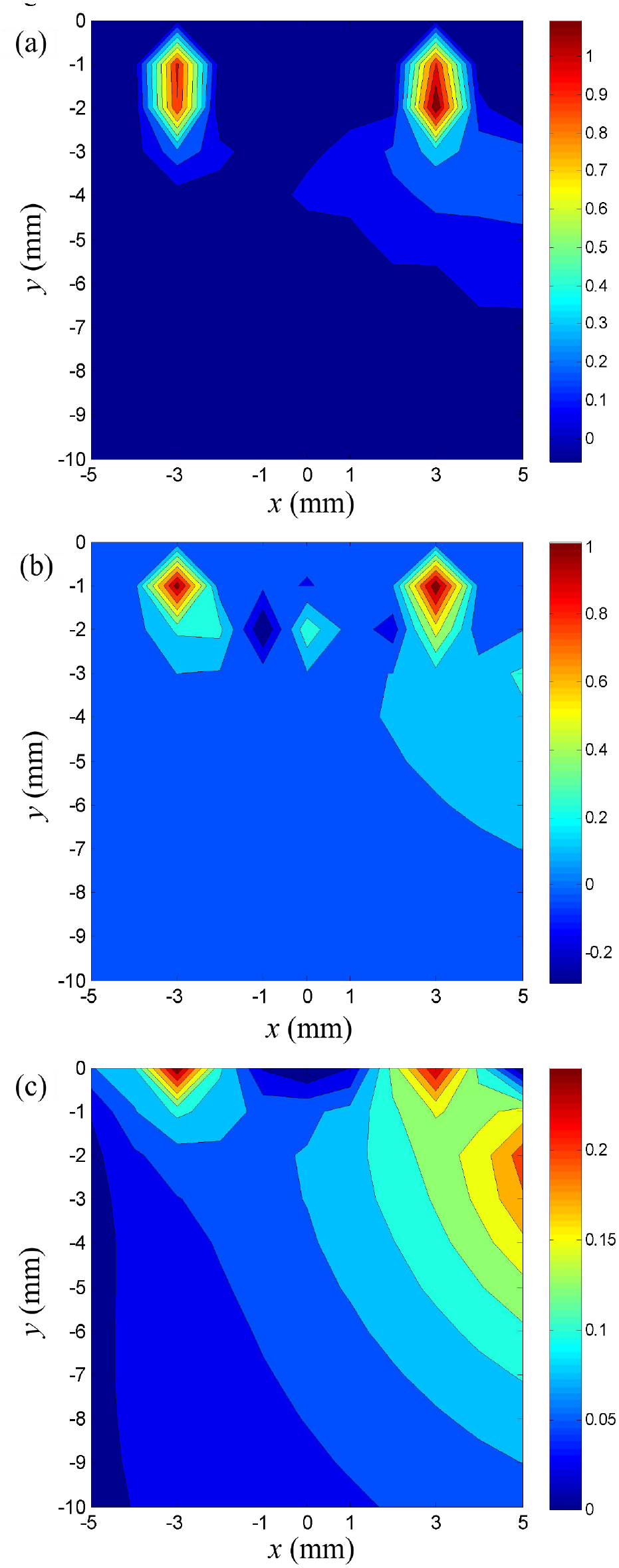
Image representation of recovery dipoles strength after the process of the reduced space inversion, the magnetic fields data for inversion was measured under a single lift-off value: (a) the lift-off value l is 0.5 mm, (b) l = 1.0 mm, and (c) l = 3.0 mm.
We can see that the capability of reduced space reversion to image the dipoles with better accuracy than the first inversion from Figure 5. However, the inversion image quality is influenced by the lift-off value. The reason is that the surface dipole exhibits more influence on magnetic flux leakage signals than that in the inner. When the magnetic flux leakage data are measured with a small lift-off value, the contributions of dipoles located deeper are easily buried under the dipoles located nearer to the surface. Therefore, the inversion image can only show the dipoles well which are near to the specimen surface. When the measurement performed with a bigger lift-off value, the contributive proportion of dipoles which located deeper will increase and the inversion image can show the dipoles located deeper. However, the coefficient K ij corresponding to deep sources are much alike and it was difficult to distinguish one from another and the inversion images were somewhat out of focus.
Magnetic field data measured with multiple lift-off
When the distance from dipole locations to the scanning point increase, the coefficient value decrease fast, however, the decreased tendency are more and more slowly. That means, the smaller lift-off, the shallower exploration depth. In turn, the bigger lift-off, the hazer of the reproduction of the dipoles strength image. Hence, we can establish the nonlinear equation as follows:

where
where
The generalized inverse minimizes not only the norm of RMS, but also the norm of the solution. In this case, it will provide us with the best estimate of the magnetic dipole strength for magnetic flux leakage data measured under all lift-off values. However, we will have a larger residual error than the one obtained with the magnetic flux leakage data were measured under a single lift-off value.
Compose the
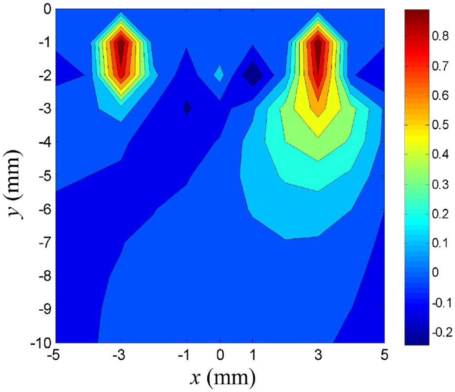
Image representation of recovery dipoles strength with the magnetic fields data for inversion were measured under multiple lift-off values.
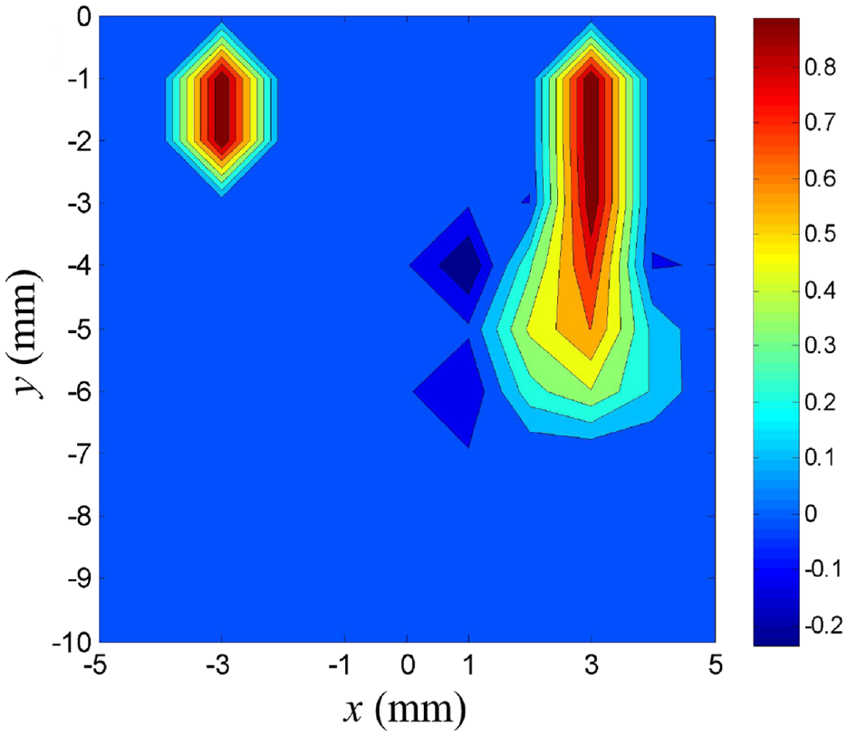
Image representation of recovery dipoles strength after the process of the reduced space inversion, the magnetic fields data for inversion was measured under multiple lift-off values.
In order to quantify the quality of the inverted image, the correlation coefficient γ is defined as follows16,17:
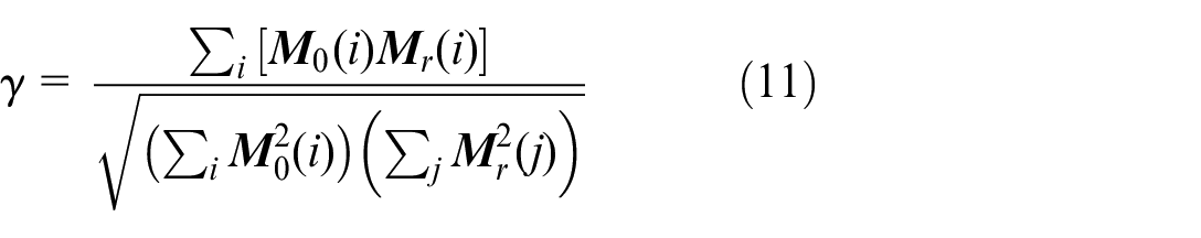
where
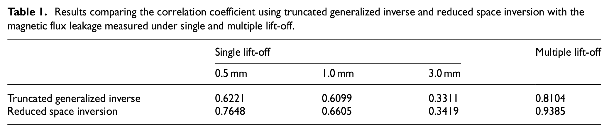
Results comparing the correlation coefficient using truncated generalized inverse and reduced space inversion with the magnetic flux leakage measured under single and multiple lift-off.
Experiments
To demonstrate the application effect in the MMM test, the new method are applied to imaging rectangular crack defects. The specimen is made of medium carbon #45 steel and the shape and dimension of specimen are shown in Figure 8. Three rectangular grooves are machined in the test specimen to simulate the actual defects. The widths of the grooves are 1.0 mm and the depths are 2.0, 4.0, and 6.0 mm respectively. The MMM test experiments are conducted on a 3D mobile platform, and magnetic signals are measured by tri-axial magnetic sensor HMC5883L produced by Honeywell. The distance of the horizontal interval is set to 0.1 mm, and the lift-off value l of the magnetic sensor is changed from 1.5 to 3.5 mm in steps of 1 mm.
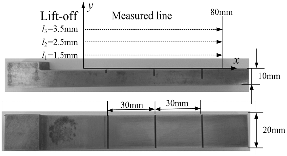
Geometry and dimensions of specimen and scanning lines.
The SMLF sifnal of cracks
The tangential component of cracks SMLF are shown in Figure 9. As Figure 9 shows, The measured data is the sum of the environmental magnetic field H0 and the scattering magnetic field H generated by crack. For the SMLF belongs to a kind of weak magnetic field signals, the environmental magnetic field must be taken into consideration. the measured signal

where
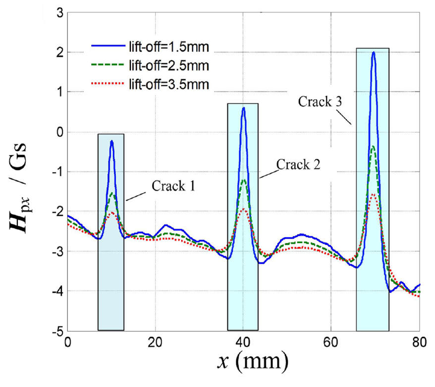
The tangential component of SMLF signals.
Since the change of magnetic field
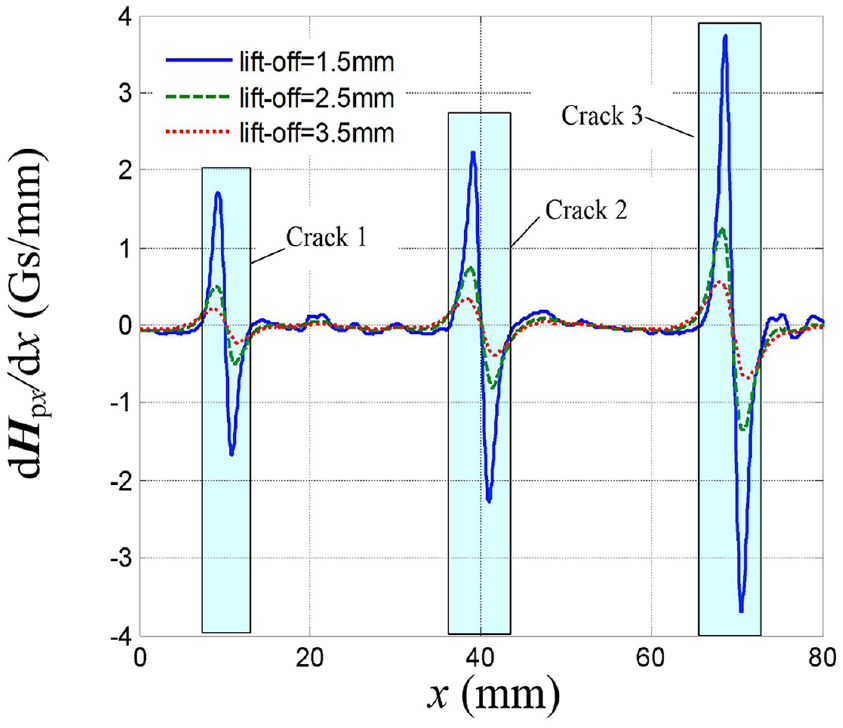
Tangential component gradient of SMLF signals.
Schemati crepresentation of the long crack defect model.
Long crack model
The long cracks can be simulated by simplified two-dimensional magnetic dipole model, and the SMLF at point p with co-ordinates (x
i
, y
i
) produced by magnetic dipole
where
where
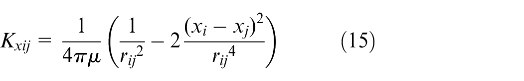
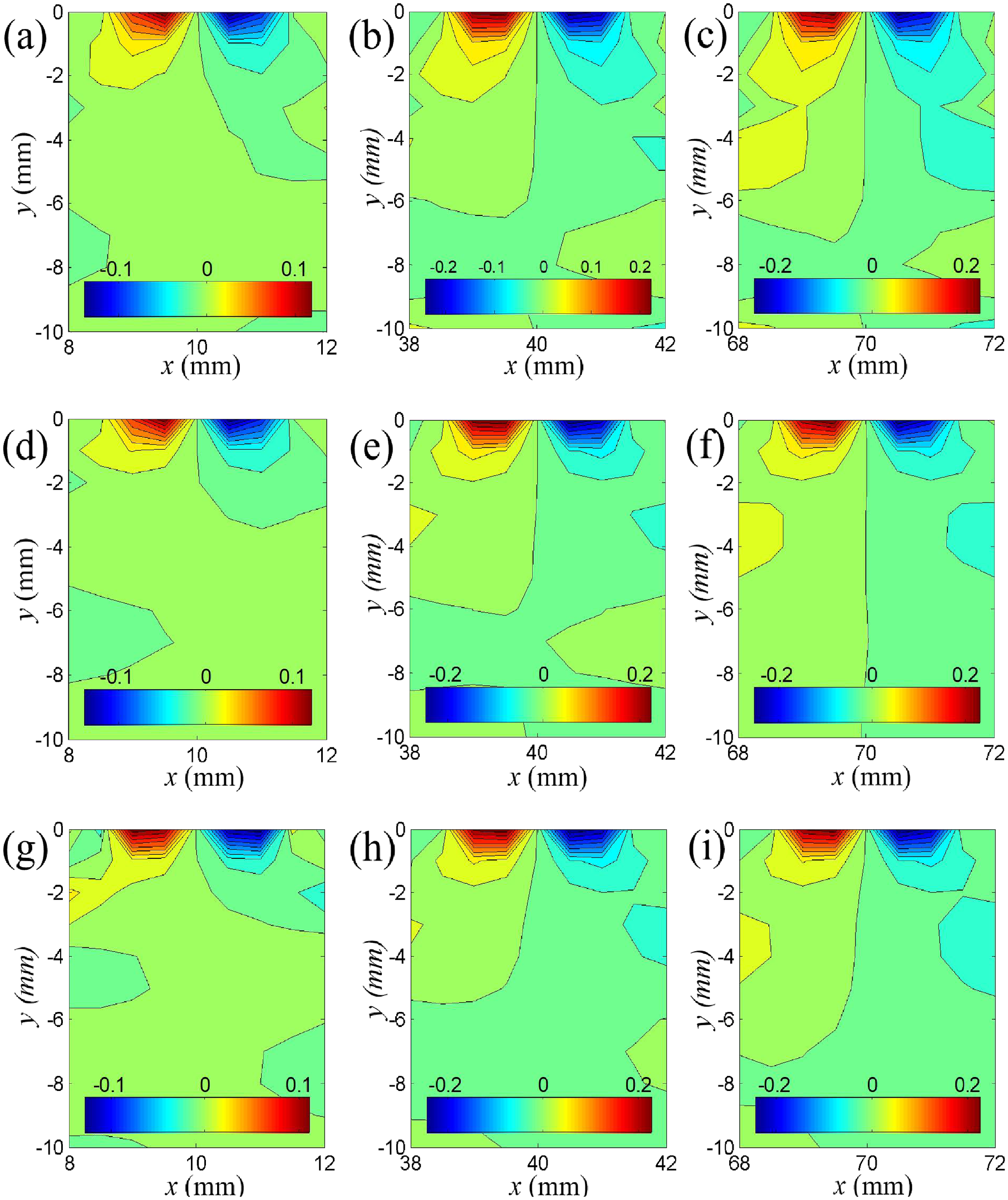
Image representation of recovery dipoles strength with the magnetic fields data measured under a single left-off value: (a) crack 1, l = 1.5 mm, (b) crack 2, l = 1.5 mm, (c) crack 3, l = 1.5 mm, (d) crack 1, l = 2.5 mm, (e) crack 2, l = 2.5 mm, (f) crack 3, l = 2.5 mm, (g) crack 1, l = 3.5 mm, (h) crack 2, l = 3.5 mm, and (i) crack 3, l = 3.5 mm.
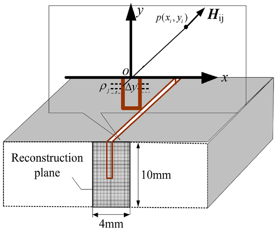
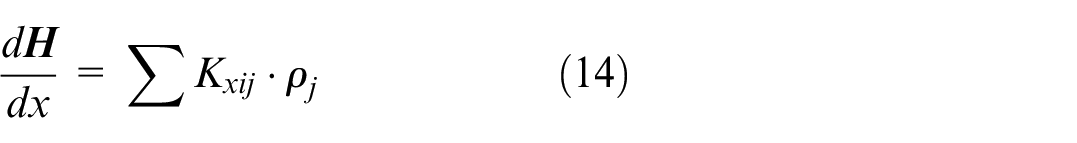
The size and position of cracks can be estimated approximately based on the gradient distribution of the tangential component of SMLF. So, as Figure 12 shows we can decrease the reconstruction plane to a size of 4 mm × 10 mm. Then, the reconstruction plane was meshed into 9 × 11 locations, in step 0.5 and 1.0 mm in x and y directions respectively. Assumed that, the magnetic dipoles are located only at the these locations and the SMLF caused by the crack can be considered as the sum of the magnetic field of these magnetic dipoles. Then, using the equation (15), we can establish the coefficient matrix
Results and analysis
First, we inverse the defect image with the magnetic data measured under a single lift-off value and multiple lift-off values respectively. The first inversion results using truncated generalized inverse directly are shown in Figures 12 and 13, where all the singular values bellow 10−5 of the biggest were truncated. It is evident that the magnetic dipoles distribute on the crack sections with opposite polarities and the dipoles strength inversed by multiple lift-off values with better accuracy than the single lift-off value one.
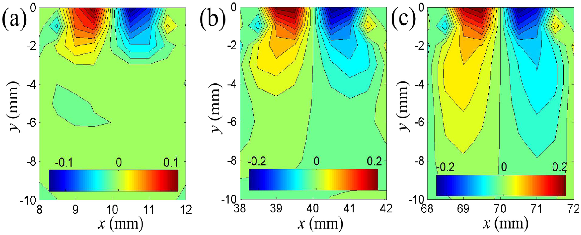
Image representation of recovery dipoles strength with the magnetic field data were measured under multiple lift-off values: (a) crack 1, (b) crack 2, and (c) crack 3.
According to the first inversion results shown in Figure 13, we set the minimum threshold
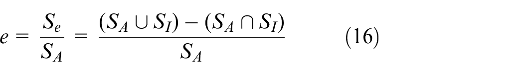
where S
e
is the cross-sectional area of inversion error,
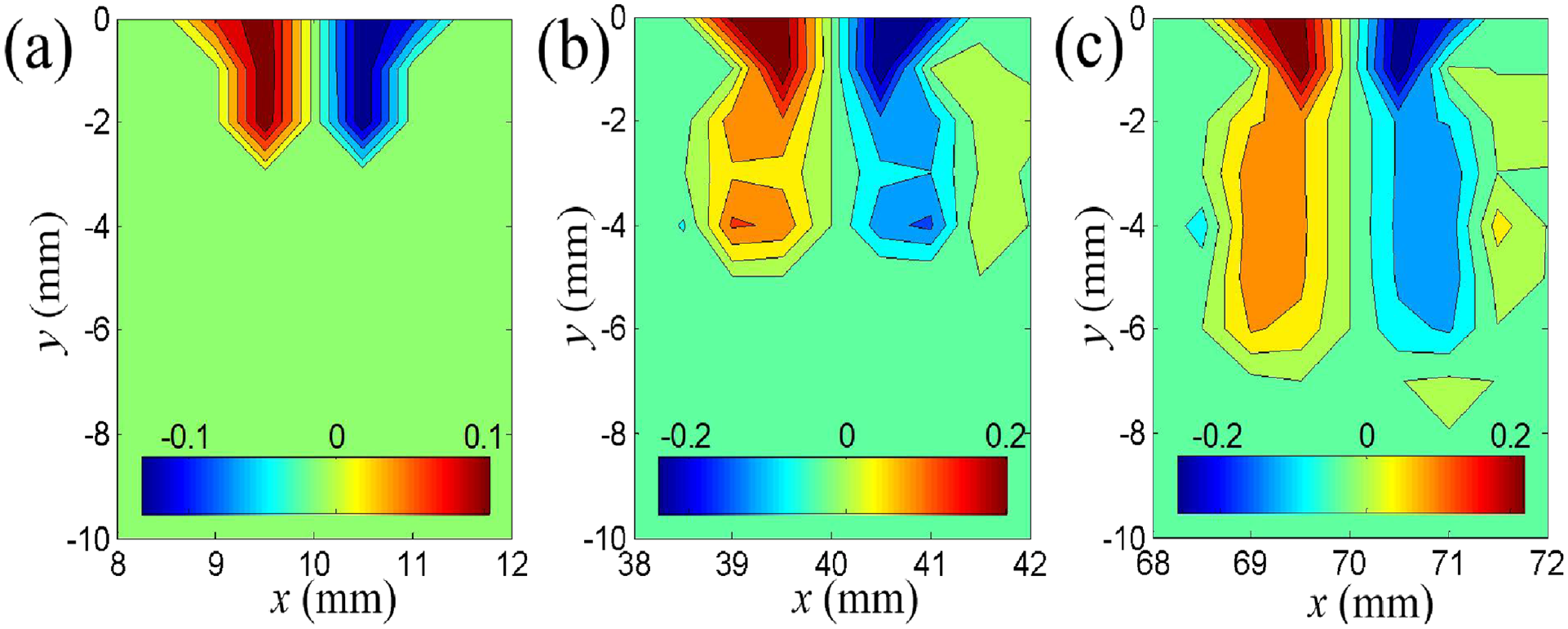
Image representation of recovery dipoles strength after the process of the reduced space inversion, the magnetic field data for inversion was measured under multiple lift-off values: (a) crack 1, (b) crack 2, and (c) crack 3.
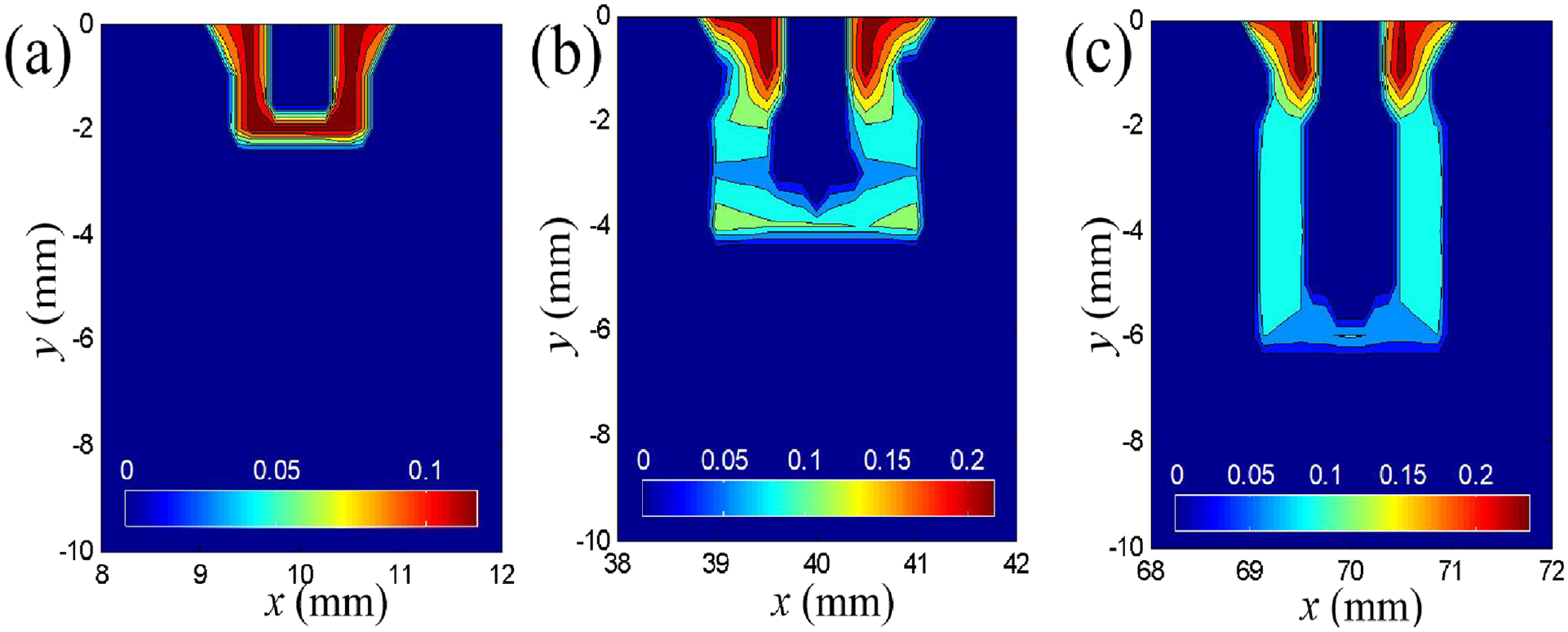
Image representation of the absolute value of recovery dipoles strength: (a) crack 1, (b) crack 2, and (c) crack 3.
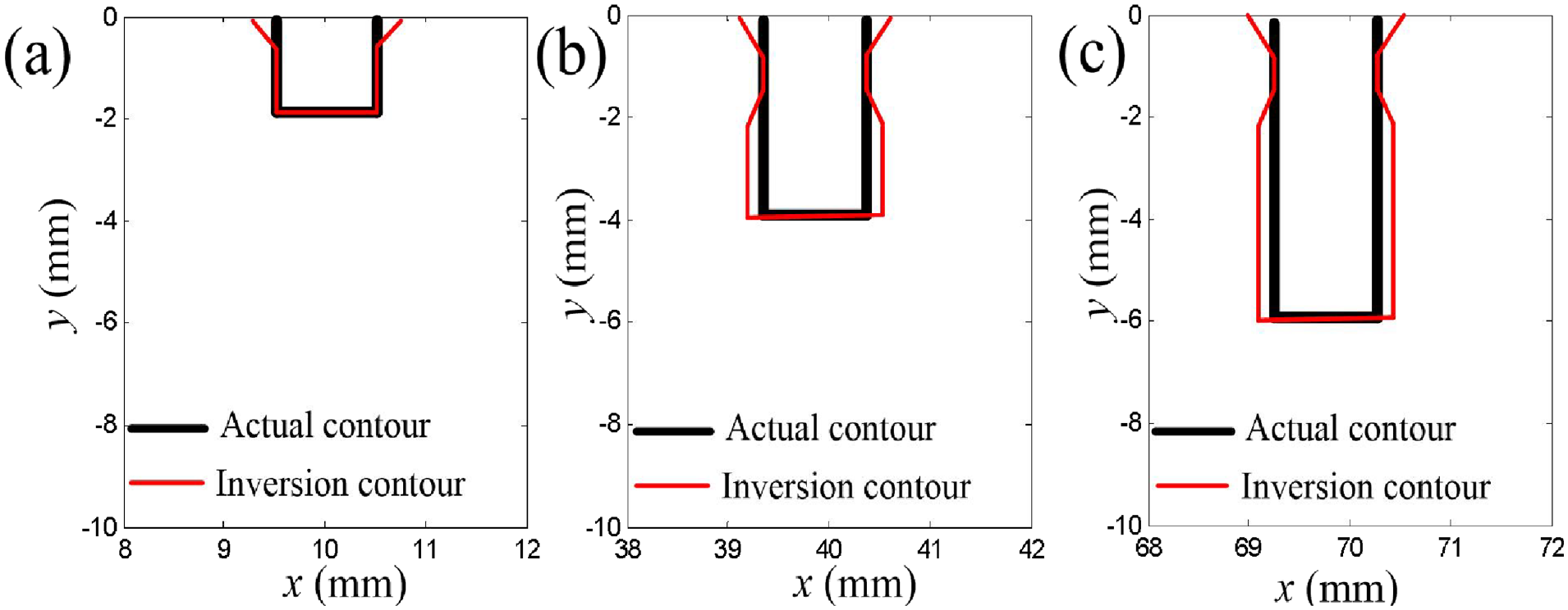
The inversion contour and actual contour of defects: (a) crack 1, (b) crack 2, and (c) crack 3.
Conclusion
Mesh the reconstruction plane into many locations and assumed that the magnetic dipoles only distributed on these locations. Then the magnetic field caused by the defect can be expressed as a linear combination of these magnetic dipoles with fixed position but unknown strength. When the magnetic field was measured, these dipoles strength can be well estimated by using truncated generalized inverse and reduced space inversion method. However, the quality of the dipole strength imaging is influenced by the lift-off value and defects depth. When the magnetic field is measured under a small lift-off value, it has advantage in imaging the dipoles in the region near the surface or the top part of defect. When the lift-off value is bigger, it has advantage in imaging the dipole located inner or the bottom part of defect. The simulation and experiment results show that, compose the magnetic data measured under different lift-off value together for inversion with better accuracy than the single one. With the image of the dipole strengths reconstructed, it will be possible to locate the defects and visualize their shapes. To verify the effectiveness of the proposed method, test pieces with the same width cracks were used. However, the width of the defect can also significantly impact the magnetic field distribution. Especially when the crack width is much larger than the lift-off value of the magnetic field sensor, the distribution of the leakage magnetic field from the defect becomes more complex, posing greater challenges to the image inversion of the defect. This is an area that requires further research.
Footnotes
Declaration of conflicting interests
The author(s) declared no potential conflicts of interest with respect to the research, authorship, and/or publication of this article.
Funding
The author(s) disclosed receipt of the following financial support for the research, authorship, and/or publication of this article: This work was supported by Hebei Provincial Natural Foundation (grant number E2015506004).
Data availability statement
Data sharing not applicable to this article as no datasets were generated or analyzed during the current study.